Design of a Test Bench for Battery...
92
Institutionen för systemteknik Department of Electrical Engineering Examensarbete Design of a Test Bench for Battery Management Report Performed at Electronic Devices at Linköping Institute of Technology by Johann Dussarrat Gael Balondrade Reg nr: LiTH-ISY/ERASMUS-A--12/0002--SE September 14, 2012 TEKNISKA HÖGSKOLAN LINKÖPINGS UNIVERSITET Department of Electrical Engineering Linköping University SE-581 83 Linköping, Sweden Linköpings tekniska högskola Institutionen för systemteknik 581 83 Linköping
Transcript of Design of a Test Bench for Battery...

Institutionen för systemteknik
Department of Electrical Engineering
Examensarbete
Design of a Test Bench for Battery Management
Report
Performed at Electronic Devices
at Linköping Institute of Technology
by
Johann Dussarrat
Gael Balondrade
Reg nr: LiTH-ISY/ERASMUS-A--12/0002--SE
September 14, 2012
TEKNISKA HÖGSKOLAN
LINKÖPINGS UNIVERSITET
Department of Electrical Engineering
Linköping University
SE-581 83 Linköping, Sweden
Linköpings tekniska högskola
Institutionen för systemteknik
581 83 Linköping

Design of a Test Bench for Battery Management
Report
Performed at Electronics Devices
at Linköping Institute of Technology
by
Johann Dussarrat & Gael Balondrade
Reg nr: LiTH-ISY/ERASMUS-A--12/0002--SE
Supervisor: Mattias Krysander, Associate Professor
Linköping University
Examiner: Atila Alvandpour, Professsor
Linköping University
Linköping, September 14, 2012


Presentation Date 2012-09-14
Publishing Date (Electronic version)
Department and Division
Division of Electronic Devices
Department of Electrical Engineering Linköpings Universitet SE-581 83 Linköping, Sweden
URL, Electronic Version http://www.ep.liu.se
Publication Title Design of a Test Bench for Battery Management
Author(s) Johann Dussarrat & Gael Balondrade
Abstract
The report deals with energy conservation, mainly in the field of portable energy, which is a subject that today raises questions around the world. This report describes the design and the implementation of a Battery Management System on the platform NI ELVIS II+ managed by the software Labview. The first aim has been on finding information about the design of the Battery Management System that corresponds to the choice of the battery itself. The system was designed completely independent with different charging methods, simulations of discharge, and its own cell balancing, as a 3 cells battery pack was used. The battery chosen was the lithium-ion technology that has the most promising battery chemistry and is the fastest growing. Several experimentations and simulations have been done, with and without cell balancing that permited to highlight that the cell balancing is mandatory in a Battery management System. Furthermore, a simulation of use of the battery in an Electrical Vehicle was made, which can lead to conclude that the Lithium-Ion battery must be managed differently to be used in the application of an Electrical Vehicle.
Keywords Battery Management System, BMS, Battery Li-Ion, Electrical Vehicle, Labview
Language
X English Other (specify below)
Number of Pages 78
Type of Publication
Licentiate thesis Degree thesis Thesis C-level Thesis D-level X Report Other (specify below)
ISBN (Licentiate thesis)
ISRN: LiTH-ISY/ERASMUS-A--12/0002--SE
Title of series (Licentiate thesis)
Series number/ISSN (Licentiate thesis)


V
Abstract
The report deals with energy conservation, mainly in the field of portable energy, which is a
subject that today raises questions around the world. This report describes the design and
the implementation of a Battery Management System on the platform NI ELVIS II+ managed
by the software Labview. The first aim has been on finding information about the design of
the Battery Management System that corresponds to the choice of the battery itself. The
system was designed completely independent with different charging methods, simulations
of discharge, and its own cell balancing, as a 3 cells battery pack was used. The battery chosen
was the lithium-ion technology that has the most promising battery chemistry and is the
fastest growing. Several experimentations and simulations have been done, with and without
cell balancing that permited to highlight that the cell balancing is mandatory in a Battery
management System. Furthermore, a simulation of use of the battery in an Electrical Vehicle
was made, which can lead to conclude that the Lithium-Ion battery must be managed
differently to be used in the application of an Electrical Vehicle.
Keywords: Battery Management System, BMS, Battery Li-Ion, Electrical Vehicle, Labview


VII
Acknowledgement
We would like to thank our supervisors Professor Atila Alvandpour and Assistant Professor
Mattias Krysander for helping us to do a project in the electronics department and for all the
valuable advices that we have gotten during the thesis.
We must not forget to thank the fabulous Linköping University that permitted us to come
and work here, but also that has offered us a very interesting subject, and provided all the
necessary equipment to be able to work in perfect condition. The university gave us an
opportunity to improve and evolve our skills in electronics, especially in the renewable
energy management area. On a more personal level, we thank our two respective families for
the interest and the encouragement and without who nothing could have been possible.
We will never forget this fantastic experience.
Johann Dussarrat and Gael Balondrade
Linköping, September, 2012


IX
CONTENTS
Introduction and theory ....................................................................................................................................... 1
1 Introduction....................................................................................................................................................... 3
1.1 Problem description .......................................................................................................... 3
1.2 Objectives........................................................................................................................... 3
1.3 Target Group ...................................................................................................................... 3
1.4 Outline ................................................................................................................................ 4
Documentations and Background .................................................................................................................. 7
2 Battery Systems background ................................................................................................................... 8
2.1 Introduction ....................................................................................................................... 8
2.2 Outline ................................................................................................................................ 8
2.3 Type Of Batteries ............................................................................................................... 8
2.4 Cell Protection .................................................................................................................. 12
2.5 Charge Control ................................................................................................................. 14
2.6 State of charge’s estimations, General’s description ..................................................... 15
2.7 State of Health estimation .............................................................................................. 22
2.8 Cell Balancing ................................................................................................................... 23
2.9 Transistor ......................................................................................................................... 27
Designs ......................................................................................................................................................................... 29
3 Hardware Design .......................................................................................................................................... 30
3.1 Introduction ..................................................................................................................... 30
3.2 Outline .............................................................................................................................. 30
3.3 Transistors used ............................................................................................................... 30
3.4 Cell balancing ................................................................................................................... 31
3.5 Charge .............................................................................................................................. 32
3.6 Enable Charge/Discharge ................................................................................................ 35
3.7 Discharge .......................................................................................................................... 37
4 Software design ............................................................................................................................................. 38
4.1 Introduction ..................................................................................................................... 38
4.2 Outline .............................................................................................................................. 38
4.3 The board ......................................................................................................................... 39
4.4 Laboratory Virtual Instrument Engineering Workbench (LabVIEW) .............................. 42

X
4.5 BMS Functions ................................................................................................................. 49
4.6 Simulation Design ............................................................................................................ 58
Simulations ................................................................................................................................................................ 61
5 Manual ................................................................................................................................................................ 62
5.1 Introduction ..................................................................................................................... 62
5.2 Initialization ..................................................................................................................... 63
5.3 Overview .......................................................................................................................... 63
5.4 Main Functions ................................................................................................................ 65
6 Experimentations ......................................................................................................................................... 70
6.1 Introduction ..................................................................................................................... 70
6.2 Auto Cell Balancing improvements ................................................................................. 70
6.3 Electrical Vehicle .............................................................................................................. 72
7 Conclusion ........................................................................................................................................................ 74
7.1 Conclusion ........................................................................................................................ 74
7.2 Future Work ..................................................................................................................... 74
References .................................................................................................................................................................. 75
Notations ..................................................................................................................................................................... 77
Components used ................................................................................................................................................... 78

1
Part I
INTRODUCTION AND
THEORY


3
1 INTRODUCTION
1.1 PROBLEM DESCRIPTION
Nowadays energy is a main problem of our planet, with fossil energies which are not an
infinite sources, humanity is forced to develop other energy system. Therefore renewable
energy systems were developed many years ago like the battery system which in addition to
be a portable source, can easily replace fossil energy in many applications. Typically batteries
are the primary option for electric energy storage like Electric road Vehicles (EV),
Uninterruptible Power Supplies (UPS), renewable energy system, and cordless electric power
tools are examples of such application. However to improve the efficiency of the battery, and
even more the new batteries, the system needs a Battery Management Systems which is used
in many battery-operated industrial and commercial systems to make the battery-operation
more efficient. But on this field, we just start to see the beginning of the possibilities of such a
system, there are many door that just ask to be opened, the market is ready to receive offers,
and all systems can be improved. That is the reason of this Project, start from zero,
considering what had been already done.
1.2 OBJECTIVES The topic of this research is to create a Test Bench for a Battery Management System able to
work with any type of battery, mainly the most recent. The common objectives to all Battery
Management Systems are to protect the cells or the battery from damage, prolong the life of
the battery, and maintain the battery in a state in which it can fulfill the functional
requirements of the application for which it was specified.
1.3 TARGET GROUP
The target group for this thesis is undergraduate and graduate engineering students with a
background from electronic engineering with an interest of learning more about renewable
energy management

4 Chapter 1. Introduction
1.4 OUTLINE
Part I This part shows an introduction to the thesis as well as the background of the project
is described.
Part II The thesis will in the second part go through the basics research and design for a
Battery Management System, it will highlight models of batteries and their
characteristics that will permit to make a choice for the bench.
Part III This part is dedicated to the design, and is divided in 2 chapters, one where the
hardware design is presented, each blocks are explained in details together with their
functioning. Secondly, the chapter presents the software design under Labview with
the platform NI ELVIS II+.
Part IV This is the final concluding part which presents the outcome of the experimentations
and their critics. The manual of the program is detailed in this part as well as the
conclusion of the thesis with some thoughts for the future work.
1.4. Outline 5
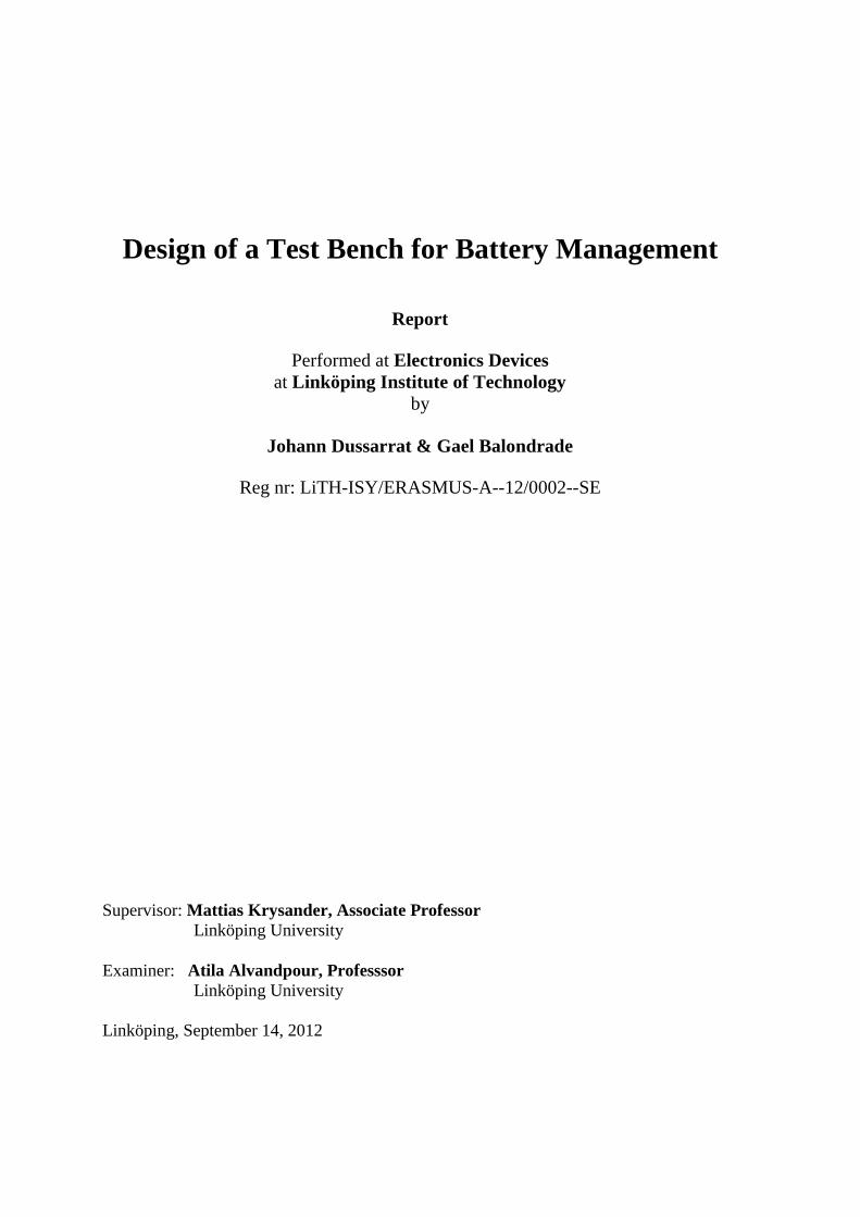
Figure 1.1: General scheme.


7
Part II
DOCUMENTATIONS
AND BACKGROUND

8
2 BATTERY SYSTEMS BACKGROUND
2.1 INTRODUCTION
This chapter presents basic information about the Battery Management System and is based
on a literature study. Many different architectures exist, but the most decisive point was to
learn what is made today, for which application, and what is possible to create during the
Master Thesis. The Battery System is divided in blocks which include a cell protection system
in charge to protect the battery and the user from any failures. But also a charge control
sytem, a State Of Charge system (SOC), a State Of Healt system (SOH), and a cell balancing
system. Every blocks are detailed in the following sections.
2.2 OUTLINE
This chapter will divide the research in sub chapters. Section 2.3 will go through the multiple
types of batteries in order to make the best choice of it for the project. In section 2.4, the cell
protection will be presented in detail, which highlights the methods to protect the user of a
consequence from a battery failure. The next point will concern the charge control, explain
different way to charge a battery. The two next sections will deal with the State Of Charge. A
description of it will be done before with the multiple methods to estimate it, followed by a
concrete example. The last point will show the cell balancing.
2.3 TYPE OF BATTERIES
Batteries are divided in two categories, the non-rechargeable battery, created to be used one
time and discarded. They are called primary cells. The second category is the one that will be
used in the project, the rechargeable battery, which is designed to be discharged-recharged
multiple times, called secondary cell. As the purpose of the project is to develop a BMS test-
bench, the idea was to focus on the most common battery and the one that will be used in the
future. Depending on this, four types of battery emerged, as followed.

2.3. Type Of Batteries 9
Nickel-Metal Hybrid Battery
The Nickel-Metal Hybrid battery, Figure 2.1, is the most common rechargeable battery and it
is used in many common electronics. However the Table 2.1 [15, 16, 17] shows that its
characteristics are not a large advantage to compare with the others batteries conceptions.
Table 2.1: Summary data of the Nickel-Metal Hybrid Battery.
Energy Power Density
Charge/ Discharge Efficiency
Self-Discharge Cycle Durability
Nominal Voltage
Specific Density
60-120 W.h/kg
140-300 W.h/L
250-1000 W/kg
66% 2% per month 500-1000 1.2 V
Advantage: -Cheapest
Inconvenient: -Low Energy Density
Domain of Application: Domestics electronic, Hybrids Vehicles.
Lithium-Ion Battery
The lithium-ion technology, Figure 2.2, has the most promising battery chemistry and is the
fastest growing. This battery has low maintenance battery, an advantage that most other
chemistries do not have. The Table 2.2 [14] highlights the specifications of the battery itself.
Table 2.2: Summary data of the Lithium-Ion Battery.
Energy Power Density
Charge/ Discharge Efficiency
Self-Discharge Cycle Durability
Nominal Voltage
Specific Density
100-250 W.h/kg
250-620 W.h/L
250-340 W/kg 80-90 % 8% per month @ 21°C 15% per month @ 40°C 31% per month @ 60°C
500-1000 1.2 V
Advantage: -Light
-Bigger Energy Density
Inconvenient: -More expensive
Domain of Application: Refillable Vehicles, laptops...
Figure 2.1: Nickel-Metal Hybrid Battery.
Figure 2.2: Lithium-Ion Battery.
10 Chapter 2. Battery System Background
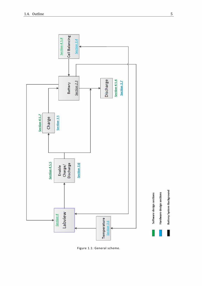
Lithium-Ion Polymer Battery
The lithium-Ion Polymer battery, Figure 2.3, differentiates itself from the classic Li-Ion
battery systems in the type of electrolyte used. This electrolyte looks like a plastic film that
does not conduct electricity but allows ions exchange. The table 2.3 [14, 15, 16] shows the
caracteristics.
Table 2.3: Summary data of the Lithium-Ion Polymer Battery.
Energy Power Density
Charge/ Discharge Efficiency
Self-Discharge Cycle Durability Nominal Voltage
Specific Density
130-200 W.h/kg
300 W.h/L 7100 W/kg
99.8% 5% per month More than 1000 3.7 V
Advantage: -Great Power Density
-Can choose the form
Inconvenient: -Low Energy Density
Domain of Application: Cellular phones, watches...
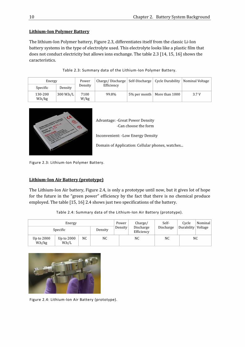
Lithium-Ion Air Battery (prototype)
The Lithium-Ion Air battery, Figure 2.4, is only a prototype until now, but it gives lot of hope
for the future in the “green power” efficiency by the fact that there is no chemical produce
employed. The table [15, 16] 2.4 shows just two specifications of the battery.
Table 2.4: Summary data of the Lithium-Ion Air Battery (prototype).
Energy Power Density
Charge/ Discharge Efficiency
Self-Discharge
Cycle Durability
Nominal Voltage
Specific Density
Up to 2000 W.h/kg
Up to 2000 W.h/L
NC NC NC NC NC
Figure 2.3: Lithium-Ion Polymer Battery.
Figure 2.4: Lithium-Ion Air Battery (prototype).

2.3. Type Of Batteries 11
The Table 2.5 highlights and informs about the energy given by the Gasoline or the Uranium.
Table 2.5: Summary data of the Gasoline and Uranium.
Energy Power Density
Charge/ Discharge Efficiency
Self-Discharge Cycle Durability Nominal Voltage
Specific Density
Gasoline 12000 W.h/kg
10000 W.h/L
NC NC NC NC NC
Uranium 22GW.h/kg 430GW.h/L NC NC NC NC NC
The table permits to compare it with the one given by a battery. We can see that the fossil
energy source is much more effective than a battery, but there is evidence now that it creates
more problems connected with pollution and environment. The first battery used for the
project will be the Lithium-Ion battery, because it is a cell very common, not expensive, and
its future in a short time.

12 Charpter 2. Battery System Background
2.4 CELL PROTECTION The Cell protection was invented to protect the cells from out of operating conditions and to
protect the user from the consequences of battery failures. One of the main functions of the
Battery Management System is the cell protection, above all when it is external to the battery.
The degree of protection varies depending on the application or the type of the battery
(chemistries). In the case of the project, Lithium-ion batteries need special protection and
control circuits to keep them within their predefined voltage, current and temperature
operating limits. Furthermore, the consequences of failure of a Lithium-ion cell could be quite
serious, possibly resulting in an explosion or fire.
The cell protection is made for:
Excessive current during charging or discharging. Short circuit Over voltage - Overcharging Under voltage - Undercharging High ambient temperature Overheating - Exceeding the cell temperature limit Pressure build up inside the cell System isolation in case of an accident
Figure 2.5 and Figure 2.6 illustrate how the safety devices are specified to protect the cells
from out of tolerance conditions by constraining the cells to a safe working zone.
The current is represented on the axe X, and the temperature on the axe Y. The red areas are
specified by the cell manufacturers as "No go" areas where cells will most likely be subject to
permanent damage. Theoretically the cell could work in any of the remaining operating
space, however this allows no margin of error and in practice protection devices limit the
cells operating conditions to a smaller "safe" operating zone shown here in green. The white
area between the safe zone and the failure zone represents the design safety margin. The
diagram Figure 3.5 shows three protection schemes providing two levels of protection from
both over-current and over temperature. If one fails the other one is there as a safety net.
Figure 2.5: Current Protection.

2.4. Cell Protection 13
Thermal Fuse: High temperatures can cause all cells to fail. The thermal fuse will shut down the
battery if the temperature exceeds the predetermined limit.
Resettable Fuse: The line “resettable fuse” indicated in the diagram Figure 2.5 provides on-
battery over-current protection. It has a similar function that the thermal fuse but after
opening it will reset once the fault conditions have been removed and after it has cooled
down again to its normal state. The fuse is triggered when a particular temperature is
reached. The temperature rise can be caused by the resistive self-heating of the thermistor
due to the current passing through it, or by conduction or convection from the ambient
environment. Then it can be used to protect against both over- current and over-temperature.
Electronic Protection: Normally, over-current protection is supplied by a current sensor
which detects when the upper current limit of the battery has been reached and interrupts
the circuit. When the specified current limit has been reached the sensing circuit will trigger a
switch which will break the current path. The switch can be a relay or a semiconductor
device. Relays can switch very high currents and provide very good isolation in case of a fault,
they are cheap, but they are very slow to operate. FET switches are normally used to provide
fast acting protection but they have a current limitation and are very costly for high power
applications.
Figure 2.6 shows a scheme for under and over-voltage, as well as temperature protection.
Figure 2.6: Voltage protection.
This example also shows interaction with the charger. Batteries can be damaged both by
over-voltage which can occur during charging and by under-voltage due to excessive
discharging. This scheme puts voltage limits for charging and discharging. Batteries (lithium
ion)can be particularly vulnerable to overcharging. By providing the charger with inputs from
voltage and temperature sensors in the battery, the charger can be cut off when the battery
reaches predetermined control limits.

14 Charpter 2. Battery System Background
2.5 CHARGE CONTROL As introduce before, the charging method is an essential feature of the BMS. A battery can be easily damaged by an inappropriate charging than by any other cause.
Three main functions of the charger:
Charging Stabilizing (Optimizing the charging rate) Terminating (know when to stop)
The purpose of good charging is to be able to detect when the reconstitution of the active chemicals is complete and to stop the charging process before any damage is done. Detecting this cut-off point and terminating the charge is critical in preserving battery life. In the simplest of chargers this is when a predetermined upper voltage limit, often called the termination voltage has been reached. If for any reason there is a risk of overcharging the battery, either from errors in determining the cut-off point or from abuse this will normally be accompanied by a rise in temperature. The temperature signal, or a resettable fuse, can be used to turn off or disconnect the charger when danger signs appear to avoid damaging the battery.
Charging Methods:
Constant Voltage: A constant voltage charger (DC power supply) provides the DC voltage to charge the battery. The lead-acid cells used for cars and backup power systems typically use constant voltage chargers.
Constant Current: Constant current chargers vary the voltage they apply to the battery to maintain a constant current flow, switching off when the voltage reaches the level of a full charge.
Pulsed charge: The charging rate (based on the average current) can be precisely controlled by varying the width of the pulses, about one second. During the charging process, short rest periods of 20 to 30 milliseconds, between pulses allow the chemical actions in the battery to stabilize by equalizing the reaction throughout the bulk of the electrode before recommencing the charge. This enables the chemical reaction to keep pace with the rate of inputting the electrical energy. It is also claimed that this method can reduce unwanted chemical reactions at the electrode surface such as gas formation, crystal growth and passivation.
Burp charging or Negative Pulse Charging: it is used in conjunction with pulse charging, it applies a very short discharge pulse, typically 2 to 3 times the charging current for 5 milliseconds, during the charging rest period to depolarize the cell. These pulses move out any gas bubbles which have built up on the electrodes during fast charging. The diffusion of the gas bubbles is known as "burping".
Trickle charge: Trickle charging is designed to compensate for the self-discharge of the battery. The charge rate varies according to the frequency of discharge. In some applications the charger is designed to switch to trickle charging when the battery is fully charged.
Random charging: All of the above applications involve controlled charge of the battery, however there are many applications where the energy to charge the battery is only available, or is delivered, in some random, uncontrolled way.

2.6. State Of Charge’s estimations, general’s description 15
2.6 STATE OF CHARGE’S ESTIMATIONS, GENERAL’S DESCRIPTION
The state of charge (SOC) is one of the most important parameters that are required to
ensure safe charging. SOC is defined as the rated capacity of the battery. SOC provides the
current state of the battery and enables batteries to be charged and discharged at a level
suitable for battery life enhancement. Failure to control SOC, leading to conditions, can
degrade the ability of the battery-pack to subsequent power transients. Li-ion batteries are
less tolerant of abuse than other battery chemistries, so they particularly require monitoring
of charge status to ensure that no under- or over-charging is occurred. The SOC definition, in
its simplest form, is the ratio between the saved energy in the battery and the total energy
that can be saved in the battery. In recent years, substantial effort has focused on the
development of the methods for estimating the SOC. A wide variety of researches which have
been done for estimate this status rely upon many parameters:
Open Circuit Voltage of the battery (OCV)
Current during charge and discharge states of the battery
Internal impedance of the battery
Electrochemical dynamics of the battery
2.6.1 ESTIMATIONS BASED ON OPEN CIRCUIT VOLTAGE
Description
These methods [5, 7] are based on Figure 2.7 witch shows the variations of the voltage during
charge and discharge state of the battery (li-ion).
In ideals conditions, an OCV refers to one and only one state of charge, but some parameters
could change the graph and skew the result of the measures. That’s why these methods
should integrate, in the estimation algorithm, some parameters of the electrochemical
reactions (the temperature, the State of health…) to improve their accuracy.
Figure 2.7: OCV Curve.

16 Charpter 2. Battery System Background
Another problem that could appear is the hysteresis curve during charge and discharge cycle.
It changes the voltage between the two cycles, as visible in Figure 2.8.
Another problem that could appear is the hysteresis curve during charge and discharge cycle.
It changes the voltage between the two cycles, as visible in Figure 2.8.
In short, the Open Circuit Voltage based estimations has many of disadvantages that could be
fix by integrate savant algorithms using some more parameters. But the main problem is that
we have to switch off the battery to get the OCV.
Advantages / Disadvantages
The main disadvantages of these methods are: Internal parameters sensibility
Great accuracy required for lithium batteries
Open circuit require to switch off the battery to get the OCV.
The main advantages of these methods are the low cost and the easy implantation. Needs
Voltages Sensors: accuracy depending of the battery type.
Figure 2.8: Schematic diagram of the hysteresis influence
on batteries.

2.6. State Of Charge’s estimations, general’s description 17
2.6.2 CURRENT INTEGRATION
Description
This estimation [6, 7] is based on
the current which flow in the
battery. Also named Coulomb
counting, the principle is to
count the charges and after a
define numbers we know that
the battery is charged or
discharged. The Figure 2.9
illustrates this method.
The problem is that the current
sensors must have a good
accuracy Another problem is
that a wrong initialization will
not be fixed, as it is visible in
Figure 2.10 The self-discharge of
the battery could also be a
problem.
These problems could be fix by recalibrate the measurements at full charge or full discharge.
This is the most common estimation because of the low cost. It is also generally used as
reference for the other estimations.
Figure 2.9: Test of currrent integration method.
Figure 2.10: Coulomb Counting Estimation Behavior.

18 Charpter 2. Battery System Background
There are few ways to estimate the SOC by the coulomb counting methods, but two seems to
be the most common:
by Software
by dedicated Hardware Figure 2.11: Single-Phased Multifunction Metering IC
In Figure 2.12, we can see after one
charge cycle, calculated Ah value by using
Single-Phase multifunction metering IC
is more close to Ah value calculated by
charge and discharge equipment, as well
as with less cumulative errors, compared
with value calculated by software
integration method.
Advantages / Disadvantages
The main disadvantages of these methods are:
Self-discharge sensibility
Great accuracy required to reduce errors
Recalibration points required
On the other hand, these methods could be better if all the imperfections are fixed by a great
accuracy to reduce cumulated errors. It can be used for all types of batteries.
Needs
As the current measurement is the main part of this method, the main requirement is to have
an extreme accuracy on the current sensor to prevent large errors.
Figure 2.11: Schematic of the Dedicated Hardware solution.
Figure 2.12: Comparison of calculed values.

2.6. State Of Charge’s estimations, general’s description 19
2.6.3 MODELLING WITH THE KALMAN FILTER
Description
This method [2, 4, 12] is based on the model of the battery, and used the Kalman filter
algorithms to estimate the state of the battery. The Kalman filter estimates an OCV, and the
error is used to get the real SOC. The complexity of the algorithms is defined by the model of
the battery.
Equivalent circuit battery models Thevenin electrical model Impedance based electrical models
Nonlinear electric models
Electrochemical battery models
Dynamic Lumped parameter Models
Hydrodynamic Model
Commonly the battery is modeled by the Thevenin model (Seong-jun Lee):
A resistance Ri is used to represent the instantaneous voltage response, a resistance Rd in
parallel with a capacity Cd is used to represent the dynamic response of the battery, with this
modeling we can define some equations which will be implanted in the Kalman filter.
In Figure 2.14 the SOC estimation result accurately tracks the real SOC in spite of an initial
value error. Also, the general trend
between ampere-hour counting and
estimation is almost the same.
Advantages / Disadvantages
The main disadvantage of this method is
the complexity of the algorithm that we
have to implement to consider all the parameters and get a good accuracy in spite of
variations in some other parameters.
Needs
The requirement of this method depends of the algorithm that it’s put in the microcontroller.
Figure 2.13: Electrical model.
Figure 2.14: SOC estimation result of proposed
algorithm.

20 Charpter 2. Battery System Background
2.6.4 IMPULSE RESPONSE CONCEPT
The pulse response of the battery is captured for various levels of SOC [1]. For a given
measured input current the output voltage is calculated by convolving it with the appropriate
set of pulse responses. Comparison of the calculated voltages with the measured output
voltage creates a method to estimate the SOC. Figure 2.15 shows the shematic.
Advantages / Disadvantages
The main disadvantage of this
method is complex system to
implement to generate the
convolution of the signal. A
dedicated hardware like a
FPGA could be used to relax
the microprocessor in this
task.
Needs
Current sensor
Current pulse generator
Voltage sensor
Convolution device
Figure 2.15: Concept's schematic.
Figure 2.16: Comparison of measured output voltage for SOC
100% with differents Calculated output voltages.

2.6. State Of Charge’s estimations, general’s description 21
As a conclusion the following Table 2.6 [3] summarizes some of methods found.
Table 2.6: Methods of SOC.
Method Advantages Disadvantage Applications Fields
Look-up tables Easy to implement Offline data, sensitive to battery and operating conditions
NiCd
Current sharing method
Sensitive to battery and operating conditions
Discharge Test Easy to implement and good accuracy
Offline data, long time, modification of the state with loss of energy
Used for capacity determination at beginning of life
Physical Properties of electrolyte
Online data, information about SOH
Sensitive to temperature and impurities
Lead-Acid, ZnBr, Va
Coup de fouet Estimate the battery Lead-Acid Linear Model Online data , Easy to
implement Need reference data for fitting parameters, sensitive to battery and operating conditions
Lead-Acid, ZnBr, Ba
Impedance Spectroscopy
Information about SOH and quality
Temperature sensitive, high cost
All batteries
Internal resistance
Information about SOH, may be online
Good accuracy for short interval
Lead-Acid, Lithium, NiCd
Fuzzy logic Online method Sensitive to battery and operating conditions
Lead-Acid
Artificial Neural Networks
Online method Needs training data on same battery, Slow convergence
All batteries
Open Circuit Voltage Based
Online method, cheap Needs long rest time(current=0)
Lead-Acid, lithium, ZnBr
Coulomb counting
Online method, Accurate if enough recalibration points and good measurement
Sensitive to parasite reactions
All batteries
Modeling with Kaman Filter
Online method, dynamic algorithm
Difficult to implement with all parameters integration
All batteries
Impulse Response Concept
Online method All Batteries

22 Charpter 2. Battery System Background
2.7 STATE OF HEALTH ESTIMATION
The SOH is defined as the ability of a cell to store energy [13], source and sink high currents,
and retain charge over extended periods, relative to its initial capabilities. The knowledge of
the SOH can be used to recognize slow or abrupt degradation of the battery and to prevent a
possible failure. A variety of techniques have been reported to estimate the SOH. The most
common one, for the lithium-ion batteries, is the Impedance Spectroscopy. The knowledge of
the internal impedance permits to estimate the SOH. Other techniques use complex
algorithms to estimate internal impedance, Figure 2.17. Table 2.7 shows the variations of the
values in order of the SOH. These variations are a piece of evidence that there is a connection
between these parameters and the SOH.
Table 2.7: Values measured.
Number of Cycles
2000 1800 1400 1000 600 200
SOH(%) 76.1 82.1 86.6 90.2 95.1 99.6 L(uH) 2.4E-7 2.8E-7 4.2E-7 5.6E-7 6.3E-7 6.9E-7 RL 2.385 2.72 3.179 4.804 5.523 6.181 Q1 246.7 237.5 215.4 195.8 182.4 157.1 N1 0.7387 0.7164 0.7468 0.6693 0.6332 0.5598 R1 0.0012 0.0027 0.0086 0.0148 0.01700 0.3598 RS 0.0537 0.0497 0.0382 0.0267 0.0226 0.0126 Q2 4.413 4.198 3.327 2.312 1.698 0.879 N2 0.3612 0.3968 0.4948 0.6283 0.6724 0.7191 R2 0.0352 0.0536 0.1143 0.1997 0.2527 0.2690
Figure 2.17: Electrical model of the internal impedance.

2.8. Cell Balancing 23
2.8 CELL BALANCING
Cell balancing was created for multi-cell batteries [8, 10]. Since there are a large number of cells used, those batteries became more subject to a higher failure rate than single cell batteries. More cells are used, more the failure rate is high, and it is in this way that the cell balancing intervenes. For example in the EV or HEV applications, the voltage used varies between 200 and 300v or even more sometimes, and instead of using several batteries, just one with several serially connected cells will be used, which can become particularly vulnerable. The balancing can be divided as passive and active balancing as shown in Figure 3.18. The passive balancing methods removing the excess charge from the fully charged cell(s) through passive resistor element until the charge matches those of the lower cells in the pack or charge reference. The resistor element will be either in fixed mode or switched according the system. The active cell balancing methods remove charge from higher charged cell(s) and deliver it to lower charged cell(s). It has different topologies according to the active element used for storing the energy such as capacitor and/or inductive component as well as controlling switches
Figure 2.18: Passive and Active cell balancing topologies.

24 Charpter 2. Battery System Background
2.8.1 SHUNTING RESISTORS BALANCING
Shunting resistor cell balancing methods are the most straightforward equalization concept. They are based on removing the excess energy from the higher voltage cell(s) by bypassing the current of the highest cell(s) and wait to until the lower voltage cell(s) to be in the same level. Description:
The first method is fixed shunt resistor, as shown in Figure 2.19. This method uses continuous bypassing the current for the all cells and the values of the resistor are chosen to limit the cells voltage. It can be only used for Lead-acid and Nickel based batteries because they can be brought into overcharge conditions without cell damage. It is features are simplicity and low cost but it has continuous energy dissipated as a heat for all cells.
The second method is controlled shunting resistor, is shown in Figure
2.20. It is based on removing the energy from the higher cell(s) not
continuously but controlled using switches/relays.
It could work in two modes. -First, continuous mode, where all relays are controlled by the same on/off signal. -Second, detecting mode, where the cells voltages are monitored. When the imbalance conditions are sensed, it decides which resistor should be shunted. This method is more efficient than the fixed resistor method, simple, reliable and can be used for the Li-Ion batteries.
Advantage/Disadvantage:
Both methods can be implemented for the low power application when dissipating current is smaller than 10mA/Ah. The main disadvantage in these methods the excess energy from the higher cells is dissipated as heat, and if applied during discharge will shorten the battery’s run tim
Figure 2.19: fixed shunt
resistor.
Figure 2.20: controlled
shunting resistor.
2.8. Cell Balancing 25
2.8.2 CAPACITY SHUTTLING BALANCING METHODS
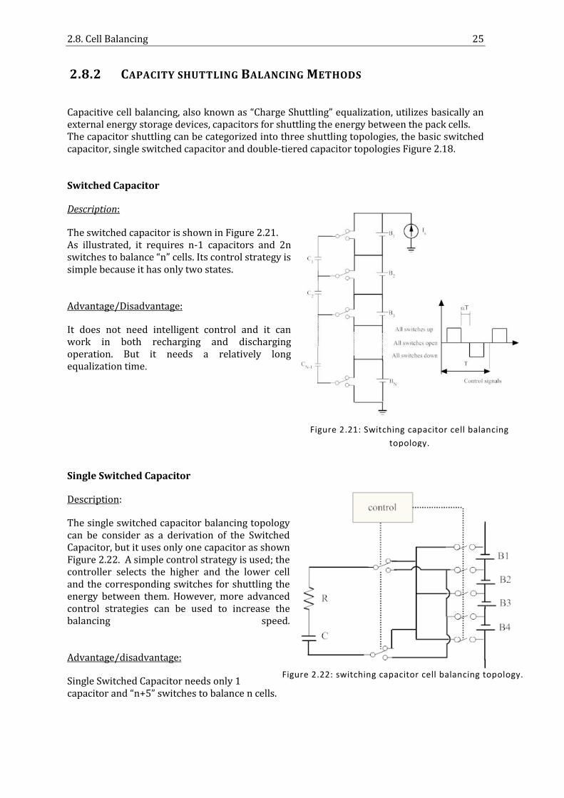
Capacitive cell balancing, also known as “Charge Shuttling” equalization, utilizes basically an external energy storage devices, capacitors for shuttling the energy between the pack cells. The capacitor shuttling can be categorized into three shuttling topologies, the basic switched capacitor, single switched capacitor and double-tiered capacitor topologies Figure 2.18. Switched Capacitor
Description:
The switched capacitor is shown in Figure 2.21. As illustrated, it requires n-1 capacitors and 2n switches to balance “n” cells. Its control strategy is simple because it has only two states. Advantage/Disadvantage:
It does not need intelligent control and it can work in both recharging and discharging operation. But it needs a relatively long equalization time.
Single Switched Capacitor
Description:
The single switched capacitor balancing topology can be consider as a derivation of the Switched Capacitor, but it uses only one capacitor as shown Figure 2.22. A simple control strategy is used; the controller selects the higher and the lower cell and the corresponding switches for shuttling the energy between them. However, more advanced control strategies can be used to increase the balancing speed. Advantage/disadvantage:
Single Switched Capacitor needs only 1 capacitor and “n+5” switches to balance n cells.
Figure 2.21: Switching capacitor cell balancing
topology.
Figure 2.22: switching capacitor cell balancing topology.

26 Charpter 2. Battery System Background
Double-Tiered Capacitor
Description:
This balancing method is also a derivation of the switched capacitor method, the difference is that it uses two capacitors tiers for energy shuttling as shown Figure 2.23. It needs “n” capacitor and “2n” switches to balance “n” cells. Advantage/Disadvantage:
The advantage of double-tiered switched capacitor over the switched capacitor method is that the second capacitor tier reduces the balancing time to a quarter. In addition, both switched capacitor topology, single switched capacitor and the double-tiered switched capacitor can work in both recharging and discharging operation.
Table 2.8 makes a summary of the advantages and disadvantages of Cell Balancing topologies.
Table 2.8: Advantages and Disadvantages of Cell Balancing topologies.
Scheme Advantage Disadvantage
1. Fixed Resistor • Cheap. Simple to implement with a small size.
• Not very effective. Inefficient for its high energy losses.
2. Shunting Resistor
• Cheap, simple to implement and Fast equalization rate. • Charging and discharging but not preferable for discharging. • Suitable for HEV but for EV a 10mA/Ah resistor specified.
• Not very effective; Relatively high energy losses • The requirement for large power dissipating resistors. • Thermal management requirements.
3. Switched Capacitor
• Simple control. Charging and discharging modes. • Low voltage stress, no need for closed loop control.
• Low equalization rate. • High switches number.
4. Single Switched Capacitor
• Simple control. Charging and discharging modes. • One capacitor with minimal switches. EV and HEV app.
• Satisfactory equalization speed. • Intelligent control is necessary to fast the equalization.
5. Double Tiered Switched Capacitor
• Reduce balancing time to quarter than the switched capacitor. • Charging and discharging modes. EV and HEV applications.
• Satisfactory equalization speed. • High switches number.
Figure 2.23: Double-tiered switching
capacitor cell.

2.9. Transistor 27
2.9 TRANSISTOR
The transistor, Figure 2.24, is an active electronic component
that can be used in 3 different ways, as a switch in logic circuits,
as a signal amplifier, and to stabilize a voltage or modulating a
signal. The transistor is a semiconductor device with three active
electrodes, which allows controlling a current that flow from the
collector to the emitter in our case.
2.9.1 BIPOLAR TRANSISTOR NPN
The NPN bipolar transistor is schematically composed of three different semiconductor
regions formed in a small block of single crystal silicon Figure 2.25.
-N area: the collector C.
-P area: the base B.
-N area: the emitter E.
The arrow indicates the direction from the junction Base - Emitter.
Figure 2.24: Transistor.
Figure 2.26: Scheme Transistor NPN. Figure 2.25: Layers Transistor NPN.

28 Charpter 2. Battery System Background
Fundamental properties of an NPN transistor
Figure 2.27 describes the currents in the transistor.
Transfer characteristic in current: Ic = f (Ib).
For Vce> 1 V, it is practically linear equation and admits: (β represents the gain in current).
Ic = β.Ib
Blocked state:
When Ib is zero, the current Ic is zero too: the transistor is off, it behaves like an opened
switch , thus:
Vce = Vcc
Saturated State:
From a certain value of the base current Ib, the current Ic remains constant (no longer
changes) even if Ib continues to increase: the transistor is saturated, it behaves like a closed
switch:
2.9.2 DARLINGTON TRANSISTOR NPN
The Darlington transistor is the combination of two bipolar transistors, resulting in a hybrid
component which further transistor characteristics. These two transistors are integrated into
the same housing. The current gain of Darlington is the product of the gains of each
transistor. The assembly is as follows Figure 2.28.
The emitter of control transistor is connected to the base of the output
transistor. The base of the control transistor and the emitter of output
transistor correspond respectively to the base and the emitter of the
Darlington. The main advantage is the high gain since the gain of the first
transistor is multiplied by the gain of the second.
Ie = Ib + Ic
Vce = 0
Figure 2.27: Currents in the Transistor.
Figure 2.28: Darlington
Transistor NPN.

29
Part III
DESIGNS

30
3 HARDWARE DESIGN
3.1 INTRODUCTION
This chapter will describe the hardware design in detail. All architectures used will be shown.
Each architecture was influenced by the primary research and as the battery chosen was the
Lithium-ion, each block is specifically designed for those types of batteries in a first time.
3.2 OUTLINE
The first section treated, shown the Transistor used during the design and for all circuits.
Afterward, the second part will be about the cell balancing followed by the charge design. The
third point of the design will be the circuit of the enable charge and discharge before finishing
with the discharging circuit design.
3.3 TRANSISTORS USED
In the design, the transistor is employed as a switch or to stabilize a current. Two types of
transistor are used, a NPN medium power transistor that can drive a current of 1A, and a NPN
silicon power Darlington with a maximum at 8A. These choices were mandatory due to the
batteries that need a “high” current to be charged or discharged in a reasonable time.
Bipolar transistor NPN (Caractieristics: Icmax=1A, Vbe=0.6V, β=250).
As it was necessary to have a power transistor that can accept a “high” current and dissipate
the heat, we were obliged to take a Darlington being given that it was the only one available
in the catalog of the components seller.
Darlington Transistor NPN (Caractieristics: Icmax=8A, Vbe=2.5V, βmin=750).

3.4. Cell Balancing 31
3.4 CELL BALANCING
Many electric applications need lot of energy (electric car, electric engine, laptop…) and there
are 2 ways to give this energy; several batteries can be used or only one battery but with
several cells inside. Then a simple battery can be a multi-cell battery, but a problem appears
over time. Those batteries become more subject to failure rate than single cell battery.
The Cell Balancing process consists to manage the current and the tension between the cells
of the battery to reduce the failure rate. There are many possibilities to achieve that, as
shown in the previous chapter, but only one was chosen. The choice was made to start with a
simple balancing, but it can still be controlled from the software Labview, and accept
different types of batteries. As described in section 2.8.1, the method is the “shunting
balancing resistor”, the design chosen is shown in Figure 3.1.
Figure 3.1: Scheme Cell Balancing.
The comparator (square) is employed to ensure the control of the balancing from Labview
with the digital output. Between the 15V and the base of the second transistor, we added a
resistance (1kΩ) to create a small current in the branch. The second transistor was associated
with another resistance (3.2Ω) to be used like an interrupter controlled from the soft.
However for cell 3, when the first transistor is elapsing the second one become immediately
elapsing too, due the low tension there is in the branch, but
enough for switching the transistor.
To solve this problem, we have put a zener diode at this place
Figure 3.2 to increase the low voltage in the branch, which
increase the threshold voltage. The transistor becomes passing
for 0.6V+Vz instead of 0.6V and the balancing can be controlled. Figure 3.2: Zener diode.

32 Chapter 3. Hardware Design
To reload each cell, we chose the current that flow in each cell. The more the cell is charged
the more the current I1 decrease, as shown in Figure 3.3, when the cell is fully
charge , and there is not current flowing to it. The value of I2 is given by the tension of
the battery as but then . The resistance 3.2 Ω, was
chosen to have , which is enough as the maximum current for the charge is 1A
due to the overheat of the power transistor, the circuit is until now limited.
Figure 3.3: Scheme Celle Balancing for one Cell.
3.5 CHARGE
The charge module shown in Figure 3.4 is composed of three sub module, the control current,
the over charge, and the command module. The purpose is to control the charge of the
battery pack with paying attention to stay in the safe area section 2.4. It can be damage by a
too high current or a too high tension. If we take for example one cell of the battery pack,
which contains three cells, the capacity of a cell is 2.3A/h and the fully charge voltage is 3.6V.
When the value’s voltage is reached, the charge turns off automatically.
Figure 3.4: Scheme Charge.

3.5. Charge 33
3.5.1 THE CURRENT CONTROL
As the battey pack is composed of 3 cells, the maximum tension Vbat will not be over 12V, in
this case we chose to fix Vcharge at 15V. Rb is a variable resistor that can vary from 0Ω to 10kΩ,
it is used to choose the charging current Ibat. Figure 3.5, the grey square represents a
Darlington power transistor as explained in section 2.9.1.
Figure 3.5: Scheme control current.
The goal of the bloc is to limit the current in the battery by choosing the value of Rb. If we
take a simple example, considering the battery pack discharged, , we keep
, then we have to change Rb to get the current wanted, here 2A. Vi is used to
generate Ib, the control current of the transistor.
, , Ib<<Ic, we neglected Ib, to get:
The datasheet of the transistor gives: and Therefore, in this example,

34 Chapter 3. Hardware Design
3.5.2 THE OVER CHARGE
The purpose of this block, Figure 3.6, is to limit the tension in the battery when it becomes
charged. Rv is a variable resistor, that vary from 0Ω to 10kΩ. A resistance of 1kΩ is added to
ensure a minimum current in the branch even if Rv is at 0Ω, in order to increase the
efficiency.
Figure 3.6: Scheme Over Charge.
Vibat is the image tension of Vbat, the tension of the battery, with a coefficient calculated as
following. It was created to have a tension higher than Vbe, in order to put the transistor
elapsing. The zener diode is added to increase the threshold voltage. represents the
value of between the nodes 1 and 3.
Until , the charge stays ON. But if Vibat becomes higher than , the
charge cut immediately due to the transistor in on state. It creates a short circuit.
The Zener diode was chosen for its low threshold voltage of 2.4V, with Vbe=0.6V, the charging
is operational until Vibat=3V.
3.5.3 THE COMMAND
Control signal is given by the platform Elvis, and controled by labview. It is a digital signal
(4.2V) sent to a bipolar transistor NPN, used like a switch to turn ON, or OFF the charge.
When 1 is sending on Labview it cuts the charge, and the value 0 turns the charging ON.

3.6 Enable Charge/Discharge 35
3.6 ENABLE CHARGE/DISCHARGE
The usefulness of this bloc is to manage the charge and the discharge for the BMS. To achieve
this task we use 2 power relays and 2 transistors as shown in Figure 3.7.
“Control 1 & 2” represents the signal
sent by Labview from the digital
output (4.2V). Control 1 is for the
charge and control 2 is for the
discharge. Both transistors are used
like switches to supply or not supply
each relay. The current sensor is
there to look at the current that flow
in the battery.
The transistors employed here are the NPN medium power transistor (1A) as there is no
more that 1A flowing inside. The relays (square) are ON when a current flow in the coil, and
OFF when there is no current.
An electromagnetic relay in Figure 3.8 consists of a coil of wire
wound around a soft iron core, an iron yoke which provides a low
reluctance path for the magnetic flux, a movable armature of iron,
and two sets of contacts. When an electric current passes through,
the coil produces a magnetic field that creates the contact. The
contact is closed when the relay is energized.
On Figure 3.9 the bottom view of the model used is
shown. Pins 1 and 2 are the coil pins. Pins 3 and 4 are the
switch pins. The tension of the coil is 12V DC with a
switching current at 10A.
Figure 3.7: Scheme Enable Charge/Discharge.
Figure 3.8: Relay.
Figure 3.9: Relay's bottom view.

36 Chapter 3. Hardware Design
For safety reasons as it is required in most BMS, we decided to add a temperature sensor to
ensure the smooth operation of the module and respect the specifications of the BMS.
The sensor is sticked to one cell, and gives in real time the value of the temperature to
Labview. The value is compared to the limited working temperature of the battery, and until
this value is under the battery limit, charge and discharge can work normaly. Otherwise it
will turn off.
The temperature sensor is mainly a zener diode whose reverse breakdown voltage is
proportional to absolute temperature. Since the sensor is a zener diode, a bias current must
be established in order to use the device. The bias circuit is shown in Figure 3.10.
As shown on Figure 3.11, the adj pin is unconnected. This pin is used to trim the diode to
calibrate it. In our case it was not needed as the temperature in the room was 25°C like the
requirement.
The output of the device is expressed as:
Where T is the unknown temperature and T0 is a reference temperature (25°C = 298 K), both
expressed in degrees Kelvin. By calibrating the output to read correctly at one temperature
the output at all temperatures is correct. Nominally the output is calibrated at 10mV/°K.
At 25°C, , this gives a coefficient
The Formula is directly implemented in Labview.
Figure 3.11: Pins. Figure 3.10: Scheme bias circuit.

3.7. Discharge 37
3.7 DISCHARGE
The design of the discharging block was chosen with 3 different values of resistance R1, R2,
R3. It is divided into three sub-blocks each composed of one comparator in order to control
the discharging current, and thus control the discharging time. Figure 3.12 shows the general
circuit.
Figure 3.12: Scheme Discharge.
The control signal is sending by Laview and permit to choose between to three resistances,
and even add a fourth value if all the signals are on “ON”. R1; R2 and R3 take respectively the
value 5Ω, 7.5Ω and10.25Ω. We can thus have seven ways to discharge the battery and study
the discharging.
Control 1 ON:
Control 2 ON:
Control 3 ON:
Control 1 & 2 ON:
Control 1 & 3 ON:
Control 2 & 3 ON:
Control 1, 2, & 3 ON:

38
4 SOFTWARE DESIGN
4.1 INTRODUCTION
The chapter software design will deal with all the design under Labview assisted by the board
Ni Elvis II+ where all the components are plugged. Labview (laboratory virtual instrument
engineering workbench) is a software generally used for command and automation
application. The choice to use this soft was motivated in a way to be the most free as possible
for different test, and in same time get a graphical environment enough readable to be use by
everyone in the future.
4.2 OUTLINE
In the first part of the chapter, the board will be described, with all the specifications,
functions and pins. Afterward, the soft Labview will be detailed in order to get sufficient
knowledge to understand the design itself that will be explained in the next section. The last
point highlights the simulations.
4.3. The Board 39
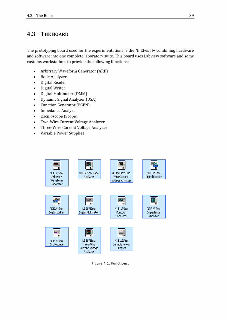
4.3 THE BOARD
The prototyping board used for the experimentations is the Ni Elvis II+ combining hardware
and software into one complete laboratory suite. This board uses Labview software and some
customs workstations to provide the following functions:
Arbitrary Waveform Generator (ARB)
Bode Analyzer
Digital Reader
Digital Writer
Digital Multimeter (DMM)
Dynamic Signal Analyzer (DSA)
Function Generator (FGEN)
Impedance Analyzer
Oscilloscope (Scope)
Two-Wire Current Voltage Analyzer
Three-Wire Current Voltage Analyzer
Variable Power Supplies
Figure 4.1: Functions.
40 Chapter 4. Software Design
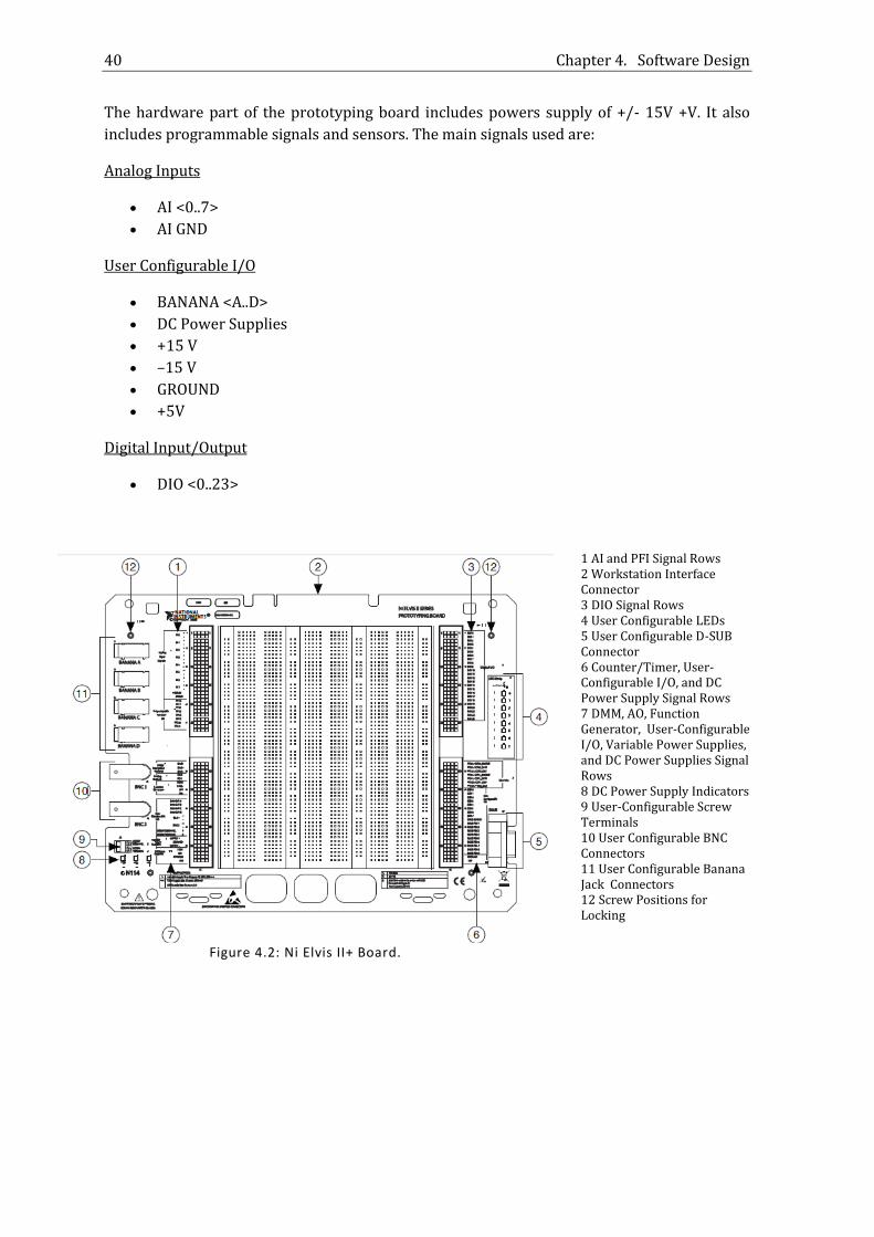
The hardware part of the prototyping board includes powers supply of +/- 15V +V. It also
includes programmable signals and sensors. The main signals used are:
Analog Inputs
AI <0..7>
AI GND
User Configurable I/O
BANANA <A..D>
DC Power Supplies
+15 V
–15 V
GROUND
+5V
Digital Input/Output
DIO <0..23>
1 AI and PFI Signal Rows 2 Workstation Interface Connector 3 DIO Signal Rows 4 User Configurable LEDs 5 User Configurable D-SUB Connector 6 Counter/Timer, User-Configurable I/O, and DC Power Supply Signal Rows 7 DMM, AO, Function Generator, User-Configurable I/O, Variable Power Supplies, and DC Power Supplies Signal Rows 8 DC Power Supply Indicators 9 User-Configurable Screw Terminals 10 User Configurable BNC Connectors 11 User Configurable Banana Jack Connectors 12 Screw Positions for Locking
Figure 4.2: Ni Elvis II+ Board.

4.3. The Board 41
4.3.1 SIGNALS SPECIFICATIONS
Analog Input:
Number of channels 8 differential or 16 single ended ADC resolution 16 bits Sample Rate Maximum 1.25 MS/s single-channel,
1.00 MS/s multi-channel Digital I/O
Number of channels 24 DI/O (Port 0) Input high voltage (VIH) 2.2 V - 5.25 V Input low voltage (VIL) 0 V - 0.8 V Output high current (IOH) –24 mA Output low current (IOL) 24 mA Positive-going threshold (VT+) 2.2 V Negative-going threshold (VT–) 0.8 V +15 V Supply
Output voltage (no load) +15 V ±5% Maximum output current 500 mA Ripple and noise 1% peak-to-peak max. Load regulation 5% Short circuit protection Resettable circuit breaker
–15 V Supply
Output voltage (no load) –15 V ±5% Maximum output current 500 mA Ripple and noise 1% peak-to-peak max. Load regulation 5% Short circuit protection Resettable circuit breaker
+5 V Supply
Output voltage (no load) +5 V ±5% Maximum output current 2 A Ripple and noise 1% peak-to-peak max. Load regulation 5% Short circuit protection Resettable circuit breaker

42 Chapter 4. Software Design
4.4 LABORATORY VIRTUAL INSTRUMENT ENGINEERING
WORKBENCH (LABVIEW)
LabVIEW is a graphical programming environment commonly used for command, test,
measurement and automation applications. The LabVIEW Laboratory language, named "G",
has become for scientists and engineers really important because they can take advantages of
I/O functionality along with the strong foundation of analysis capabilities.
The G language looks like a flow chart, joining many different icons related by wires of colors
which represent the type of data which flow through. The execution of one icon can start only
if all the data are available, in this way the diagram is ordinated and synchronized. This also
determines the order of execution of the program. This characteristic makes easier the multi-
task for multiprocessor applications. In the design process, a LabVIEW project is devised into
two pages, the Front Panel and the Black Diagram.
4.4.1 THE INTERACTIVE FRONT PANEL
Figure 5.3 shows the Booleans tools and
Figure 5.4 shows the Numerics tools. The
Front is the interactive side of the
program. It gives the possibility to see the
results on “Graphs” or to interact with the
program through controllers as Button,
Switch, numeric values, etc.
Three main plots are available Figure 4.5, 4.6, & 4.7, “Waveform
Charts”, “Waveform Graph” and “XY Graphs”.
Waveform Graph
The “Wave Charts” is most common way to display timed results
from experimentations. It permits also to write single or multi-data
points.
Waveform Charts
Compared to the previous graph, The “Wave Chart” has the
particularity to remember and display a certain number of points by
storing them in a buffer. When the buffer is full it starts to overwrite
the old points. It also permits to write single or multi-data points.
Figure 4.3: Booleans. Figure 4.4: Numerics.
Figure 4.5: Waveform Graph.
Figure 4.6: Waveform Charts.

4.4. Laboratory Virtual Instrument Engineering Workbench (Labview) 43
XY Graphs
The “XY Graphs” is a general purpose-graph which allows
plotting multivalued functions. It also permits the display
Nyquist planes, Nichols planes, S planes, and Z planes.
4.4.2 THE MAIN FUNCTIONS OF THE BLOCK DIAGRAM
The Block Diagram is the effective side of the program. This is where the icon’s flow chart.
Each icon represents a function or an executive application.
Structures
Structures are control flow statement that allow the code to be executed in a controlled way.
While The most classic structure used is the
“While”, Figure 4.8. This structure is,
executed as long as the condition of the
structure is right or false regarding of the
programming implemented. This is
commonly applied to generate the main loop
of the programming code. This structure also
allows the parallelism of execution. If two
while are in the same level of execution, the
both will be run simultaneously. The data
performs inside the “While” are not available
outside of the structure but some solutions as
a “Local Variable” could be appropriated to
avoid this problem.
Case The “Case” structure, Figure 4.9, allows the
command to have multiple values. Each value of
the command will give a special execution of the
program by a different code. If the command
type is a Boolean, the “Case” could be considered
similar as the “If”, one other famous control flow
structure unavailable in LabVIEW. This is
possible to attribute Input/Output to the
structure and they are available for each value of
the “Case”. By adding a “Shift Register”, the value
of the last iteration is saved and may be used for
the next iteration
Figure 4.7: XY Graph.
Figure 4.8: While Structure.
Figure 4.9: Case Structure.

44 Chapter 4. Sofware Design
For The “For” structure, Figure 4.10,
permits the execution of a code
with an increment of a variable,
that allows easier to browse a table
or an array for example. The “Shift
Register” is also available.
Sequence The “Sequence” structure, Figure 4.11, permits a
sequential execution of the code. The sequences are
organized in frames each frame waits for the end of the
previous one to start his code. With this structure it’s
possible to start a counter before action, or analyze data
at the end of an acquisition.
Input/Output
LabVIEW authorizes the acquisition of Inputs and generation of Outputs throughout the
service of dedicated processes.
Data Acquisition Assistant (DAQ Assistant)
Figure 4.12, the DAQ Assistant,
is a process of measuring
voltage, current, temperature
pressure, or sound. This uses a
hardware (the NI ELVIS II+ in
our case) to capture the
measure of the analog signal
from the sensors (Tension
sensors in our case).
Figure 4.10: For Structure.
Figure 4.11: Sequence Structure.
Figure 4.12: DAQ Assistant configuration window.
4.4. Laboratory Virtual Instrument Engineering Workbench (Labview) 45
Acquisition mode:
1 Sample (On Demand)
Get only one sample by iteration
1 Sample (HW Timed)
Get only one sample by timed iteration
N Samples
Get N “Samples to Read” by iteration with a “Rate” of acquisition define
Continuous
Get continuously samples saved in a buffer of N “Samples to Read” with a “Rate” of
acquisition define
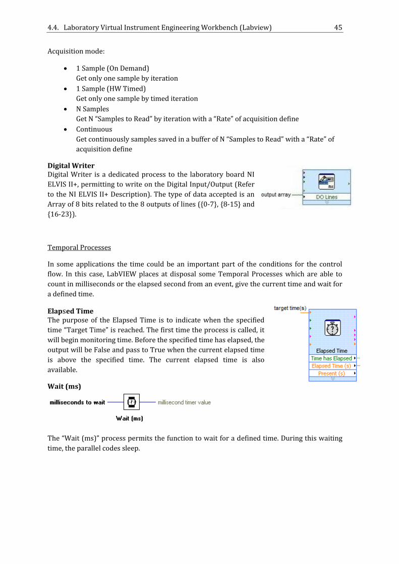
Digital Writer Digital Writer is a dedicated process to the laboratory board NI
ELVIS II+, permitting to write on the Digital Input/Output (Refer
to the NI ELVIS II+ Description). The type of data accepted is an
Array of 8 bits related to the 8 outputs of lines (0-7, 8-15 and
16-23).
Temporal Processes
In some applications the time could be an important part of the conditions for the control
flow. In this case, LabVIEW places at disposal some Temporal Processes which are able to
count in milliseconds or the elapsed second from an event, give the current time and wait for
a defined time.
Elapsed Time The purpose of the Elapsed Time is to indicate when the specified
time “Target Time” is reached. The first time the process is called, it
will begin monitoring time. Before the specified time has elapsed, the
output will be False and pass to True when the current elapsed time
is above the specified time. The current elapsed time is also
available.
Wait (ms)
The “Wait (ms)” process permits the function to wait for a defined time. During this waiting
time, the parallel codes sleep.

46 Chapter 4. Software Design
Wait until next ms multiple
The “Wait until next ms multiple” process permits the function to wait until the next
occurrence of the defined millisecond multiple.
Tick count
The “Tick Count” process returns a 32-bit number (0 to 4 billion/two months) in millisecond
of a free running counter at the time the VI wakes up.
4.4.3 DATA COMMUNICATION PROCESSES
When the program is running, it could be interesting to save in a file, the data acquired or
wired through local variables. For that, LabVIEW places at disposal some Data
Communication Processes.
Local Variable A “Local Variable” permits to write to or read from a control or indicator. Writing to a local
variable is similar to passing data to any other terminal. For example, as explain previously,
the data are not available during the looping of a “While” from the outside of the loop. The
solution is to link the values between the loops by using “Local variable”.
Saved Files Usually after a series of experimentations
the gotten values, are saved in a file that
could be archived for later comparisons or
be open in another software, more
powerful in the analyze of result. To do
that, LabVIEW places at disposal some
Processes dedicated to the data backup.
One of those is, “Write To Measurement
File”, giving the possibility to write a file
containing the all values of the experimentations in progress or finished. This file is readable,
for example, by EXCEL. It is also possible to read the saved data with the process “Read from
Measurement File”.
Another solution is “Write to Spreadsheet File” permitting to save the data in an .ASCII file
which can be opened in Matlab by a simple command: “>>LOAD filename”.

4.4 Laboratory Virtual Instrument Engineering Workbench (Labview) 47
4.4.4 MATLAB LINKS
For a better exploitation of results, LabVIEW permits to link the program with Matlab, a good
analyze tools. For that, it is possible to implant a Matlab Script.
Matlab Script
The “Matlab Script”, Figure 4.13, could be
interpreted as a process with specific
Input/Output which depending of the “Matlab
Script” as for an equation. The “Matlab Script”
authorizes to use the entire capabilities of
Matlab.
Palettes of functions
Labview places also at disposal some palettes of classic functions, Figure 4.14, 4.15, and 4.16.
Boolean palette
Figure 4.14: Boolean Palette
Numeric palette
Figure 4.15: Numeric Palette
Figure 4.13: Matlab script.
48 Chapter 4. Software Design
Comparison palette
Figure 4.16: Comparaison Palette.
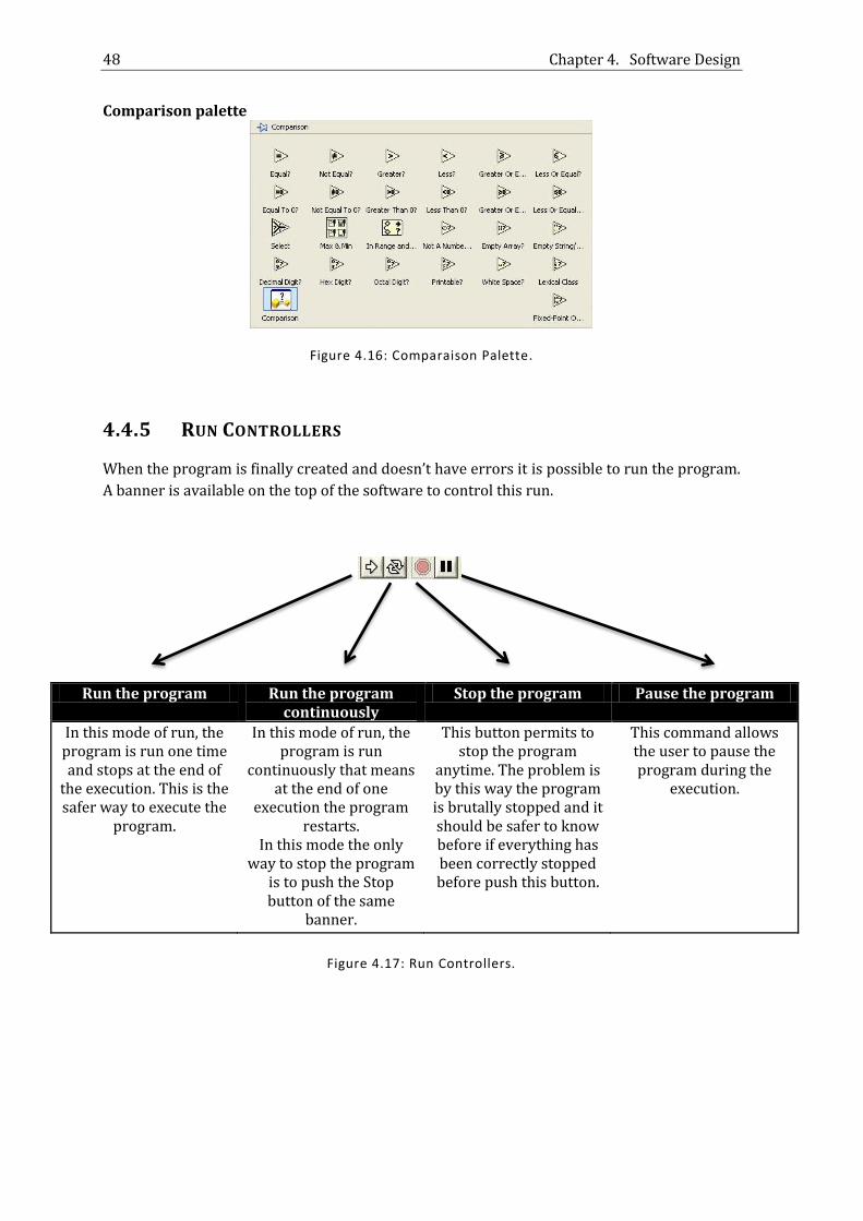
4.4.5 RUN CONTROLLERS
When the program is finally created and doesn’t have errors it is possible to run the program.
A banner is available on the top of the software to control this run.
Run the program Run the program continuously
Stop the program Pause the program
In this mode of run, the program is run one time and stops at the end of
the execution. This is the safer way to execute the
program.
In this mode of run, the program is run
continuously that means at the end of one
execution the program restarts.
In this mode the only way to stop the program
is to push the Stop button of the same
banner.
This button permits to stop the program
anytime. The problem is by this way the program is brutally stopped and it should be safer to know before if everything has been correctly stopped before push this button.
This command allows the user to pause the program during the
execution.
Figure 4.17: Run Controllers.

4.5. BMS Functions 49
4.5 BMS FUNCTIONS
4.5.1 GENERAL DESCRIPTION
All BMS functions, are implemented in the biggest one, the “Main” function, Figure 4.18. This
function permits to handle the global program by steps: Initialization, Main Code, Post
treatment and End of Simulation. To do that, a sequence structure is used. All those loops are
stoppable by a “Stop” button in the Front Panel or the end of the simulation time defined by
the Boolean local variable “Time has Elapsed” The command of the stop is transmitted by a
local variable “General Aboard”, generated by a specific loop which scans continually the
referred values.
Main Code
Acquisition
Enable Charge/
Discharge
Cell Balance Control
OCV Capture
Discharge Command
MatlabState of Charge
Time Loop
Charge Command
MatlabCell
Balancing
Initialization Post TreatmentEnd of
Simulation
Figure 4.18: Main Program.
Initialization
During this step, the program initializes the different graphs for the next execution.
Main Code
This step regroups all functions described previously.
Post Treatment
This step is launched when the program goes to the end, and uses the data acquired during
the execution to plot some values and saves data in a Matlab readable file.
End of Simulation
This step ensures that the program is stopped at the end.

50 Chapter 4. Software Design
4.5.2 ACQUISITION
With the knowledge of programming describes in the previous section, this is now possible to
create personal functions related to the BMS. In this section, all the functions created will be
explained. To improve the behavior of the program, the code has been mostly created for
parallelism tasks by using “While” loops.
Acquisition The acquisition function permits the software system to acquire the values of the hardware
system.
Tension of the battery pack
Output tension the current sensor in the battery pack
Output tension of the batteries temperature sensor
Tension of the first cell of the pack
Tension of the second cell of the pack
Tension of the third cell of the pack
Command in tension of the Pulse Modulation Charge (PMC)
In order to this, the DAQ Assistant is the main process of this function. The Acquisition mode
used is “1 Sample (On demand)”. This mode permits the function to acquire the data as fast as
possible without blocking the rest of the program. The disadvantage of this solution is that
the sampling rate is uncontrolled. After the acquisition, the sensor values are converting to
their corresponding values in the software as:
(
)
( )
The tension of cells is already usable.

4.5. BMS Functions 51
The Figure 4.19 describes the acquisition process:
Acquisition
Converting Converting Converting Converting
Current Tension Temperature Charge Command
TensionCell 2
TensionCell 3
TensionCell 1
Displaying Displaying Displaying Displaying Displaying
Writting Path « SaveFile »
Figure 4.19: Acquisition Flowchart.
4.5.3 TIME LOOP
The “Time Loop” function, Figure 4.20, governs the timing distribution of the task by giving
the time of the simulation and the “Elapsed time” in seconds from the beginning. It also
permits to report the “Time has elapsed” referring to the “Target Time (min)” given by the
user to specify the end of the experimentations. The sub-function of “Time Loop” is to
indicate when the Open Circuit Voltage (OCV) should be capture through “OVC Acquisition
ON”. The “Period OCV Acquisition” that gives the time between two captures, is given by the
user and the period of one capture is fixed to 1000 ms.

52 Chapter 4. Software Design
Elapsed Time
IFDischarging ON
orCharging ON
Elapsed Time
Every « Period OCV Acquisition »,OCV Acquisition is ON for « Delay »
Period OCV Acquisition
Delay
ELSE
DisplayingTime has elapsed
Figure 4.20: Time Loop Flowchart.
4.5.4 OCV CAPTURE
This function, Figure 4.21, is governed by the previous one, “Time Loop”, to capture the Open
Circuit Voltage of the battery pack (OCV). In a first step, if “OCV Acquisition ON” is active,
“OCV Capture” waits for 500 ms, then gets the value from the “Tension Bat”. In this way, the
acquisition is done at the lowest level of tension considering the establishment time of
tensions.
In parallel, the function compares the captured “OCV value” to the “End of Charge Value”
and “End of Discharge Value” to indicate the “End of Charge” or “End of Discharge”.
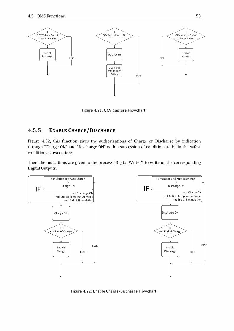
4.5. BMS Functions 53
IFOCV Value < End of
Discharge Value
IFOCV Value > End of
Charge Value
IFOCV Acquisition is ON
Wait 500 msEnd of
DischargeEnd of Charge
OCV Value gets Tension
Battery
ELSE ELSE
ELSE
Figure 4.21: OCV Capture Flowchart.
4.5.5 ENABLE CHARGE/DISCHARGE
Figure 4.22, this function gives the authorizations of Charge or Discharge by indication
through “Charge ON” and “Discharge ON” with a succession of conditions to be in the safest
conditions of executions.
Then, the indications are given to the process “Digital Writer”, to write on the corresponding
Digital Outputs.
not Discharge ONnot Critical Temperature Value
not End of Simmulation
Simulation and Auto Chargeor
Charge ON
IFnot Charge ON
not Critical Temperature Valuenot End of Simmulation
Simulation and Auto Dischargeor
Discharge ON
IF
Charge ON Discharge ON
IFnot End of Charge
IFnot End of Charge
Enable Charge
Enable DischargeELSE ELSE
ELSE ELSE
Figure 4.22: Enable Charge/Discharge Flowchart.

54 Chapter 4. Software Design
4.5.6 DISCHARGE COMMAND
The “Discharge Command”, Figure 4.23, control the discharge of the battery in 3 independent
circuits of discharge: Discharge Cell 1, Discharge Cell 2 and Discharge Cell 3. The
authorization is given according to the value of “Discharge ON” and the corresponding
“Button Discharge” or “Auto Discharge”.
In order to respect the “OCV Capture”, if an “OCV Acquisition” is in progress, the command is
given to disable all discharges. Then, the indications are given to the process “Digital Writer”,
to write on the corresponding Digital Outputs.
IFnot OCV Acquisition
IFButton Discharge 1
orAuto Discharge 1
IFButton Discharge 2
orAuto Discharge 2
IFButton Discharge 3
orAuto Discharge 3
Discharge 1 = 0Discharge 2 = 1Discharge 3 = 1
Discharge 1 = 1Discharge 2 = 0Discharge 3 = 1
Discharge 1 = 1Discharge 2 = 0Discharge 3 = 1
ELSE
IFDischarge ON
Discharge 1 = 1;Discharge 2 = 1;Discharge 3 = 1;
Figure 4.23: Discharge Command Flowchart.
The Table 4.1 describes the Array of “Digital Writer” Output:
Table 4.1: Array output.
DIO Number 1 2 3 4 5 6 7 8
Local Variable name
En
able
C
har
ge
En
able
D
isch
arge
Dis
char
ge
Cel
l 1
Dis
char
ge
Cel
l 2
Dis
char
ge
Cel
l 3
NC
NC
NC

4.5. BMS Functions 55
4.5.7 CHARGE COMMAND
The “Charge Command”, Figure 4.24, control the charge of battery, according to the value of
“Discharge ON”, by two different types: Constant Charge or Pulse Modulation Charge (PMC).
The PMC generates a pulsed charge. This command executes a serial writing of a “Defined
Array” to the output “Charge Command” with a writing period for each byte «Period of Pulse
Command ». In otherwise, for the Constant Charge, the indication to charging is always sends
to “Charging Command”.
In order to fulfill the “OCV Capture”, if an “OCV Acquisition” is in progress, the command is
given to disable the charge.
IFOCV Acquisition
IFEnable Charge
Command
IFCharge ON ELSE
Every « Period of Pulse Command »For i = 0 to 7 by 1 «Charge Command» = « Defined Array[i] »End For
Charge Command = 0
ELSE
Charge Command = 1
DefinedArray[]
Period of Pulse
Charge Command
Figure 4.24: Charge Command Flowchart.
The Table 4.2 describes the Array of “Digital Writer” Output:
Table 4.2: Array Output.
DIO Number 9 10 11 12 13 14 15 16
Local Variable name
Ch
arge
C
om
man
d
NC
NC
NC
NC
NC
NC
NC

56 Chapter 4. Software Design
4.5.8 CELL BALANCE CONTROL
According to the value of “Enable Manual Balance” and “Enable Auto Balance”, the function,
Figure 4.25, “Cell Balancing Control” has 3 modes of behavior: Cell balance Off, Manual
balance, and Auto balance.
The Manual Balance mode permits the user to balance a cell with the corresponding button
“Battery Balance”. The Auto Balance mode permits a software command to balance
automatically a cell via the corresponding local variable “Auto Balance Bat”.
IFnot Enable Manuel Balance
ornot Enable Auto Balance
IFEnable Manuel Balance
Cell Balance Cell 1 = 0Cell Balance Cell 2 = 0Cell Balance Cell 3 = 0
IFEnable Auto Balance
Cell Balance Cell 1 = Cell 1 BalanceCell Balance Cell 2 = Cell 2 BalanceCell Balance Cell 3 = Cell 3 Balance
Cell Balance Cell 1 = Auto Balance Cell 1Cell Balance Cell 2 = Auto Balance Cell 2Cell Balance Cell 3 = Auto Balance Cell 3
Figure 4.25: Cell Balance Control Flowchart.
The Table 4.3 describes the Array of “Digital Writer” Output:
Table 4.3: Array Output.
DIO Number 1 2 3 4 5 6 7 8
Local Variable name
Cel
l Bal
ance
C
ell 1
Cel
l Bal
ance
C
ell 2
Cel
l Bal
ance
C
ell 3
NC
NC
NC
NC
NC

4.5. BMS Functions 57
4.5.9 MATLAB - CELL BALANCING
This function uses a “Matlab Script” to generate the commands of the auto balance mode. At
the moment, the implemented script automatically balances a cell if it detects that another
one has a lower tension.
Script MATLAB
Tension Battery
Current Battery
OCV Value
Temperature Bat
Tension Cell 1
Tension Cell 2
Tension Cell 3
PATH fichier Matlab
Auto BalanceCell 1
Auto BalanceCell 2
Auto BalanceCell 3
4.5.10 MATLAB - STATE OF CHARGE
This function uses a “Matlab Script” to calculate the actual State of Charge. At the moment, no
script has been implemented.
Script MATLAB
Tension Battery
Current Battery
OCV Value
Temperature Battery
Tension Cell 1
Tension Cell 2
Tension Cell 3
PATH Fichier Matlab
State of Charge

58 Chapter 4. Software Design
4.6 SIMULATION DESIGN
The software design has been completed and this section is devoted to introduce and
describe how to use the test bench for three common types of experimental setup of Battery
Systems as Capacity Test, Step Response, and Electrical Vehicle.
4.6.1 CAPACITY TEST
The capacity test simulation offers the possibility to estimate the full capacity still available in
the battery pack. This information is needed in the state of health estimation. The main
purpose of this experimentation is to fully charge and fully discharge the battery pack to
estimate during discharging the value of the capacity by a current integration method.
Table 4.4: Modes.
Mode End of Discharge
End of Charge
Actions
Dis
cha
rge
0 0 Discharge Mode Auto Discharge
Discharge 1
0 1 Discharge Mode Auto Discharge
Discharge 1
1 0 Charge Mode Auto Charge
1 1 Charge Mode
Ch
arg
e
0 0 Charge Mode Auto Charge
0 1 Discharge Mode Auto Discharge
Discharge 1
1 0 Charge Mode Auto Charge
1 1 Charge Mode

4.6. Simulation Design 59
4.6.2 STEP RESPONSE
Figure 4.26 describes the step response stimulation that have permitted to get the sufficient
measurements to model the dynamics of the battery pack system. The main purpose of this
experimentation is to generate a discharge current step on the battery pack and to get in the
same time the tension values of the battery and battery Cells. Afterwards, the values are
analyzed in Matlab to estimate the model.
IFSimulation
andCapacity
Ticktime (ms)
SimulationTime (ms)
Off Time (ms)
Sim
ula
tio
n
Tim
e (m
s)
Off
Tim
e (m
s)OFF
not Autodischargenot Discharge 1
ON
AutodischargeDischarge 1
Figure 4.26: Step Response.
4.6.3 ELECTRICAL VEHICLE
The electrical vehicle simulation, Figure 4.27, permits to simulate a battery used on an
electrical vehicle in functioning and moving. That integrates steps of high accelerations,
normal acceleration, speed stabilization and brakes, considering also the regenerative brakes,
which recharge the battery during the brake step. The main purpose of this experimentation
is to manage the charge and discharge commands regarding to the time.
Figure 4.27: Electrical Vehicle Graph.

60 Chapter 4. Software Design
IFSimulation
andElectrical Vehicle
Elapsed Time (s)
End Sequence (s)
End of Brake (s)
End of High Acceleration (s)
End of Normal Acceleration (s)
Autocharge Autodischarge
Discharge 1Discharge 2
AutodischargeDischarge 2
AutodischargeDischarge 3
End
of
Bra
ke (
s)
End
of
Hig
h
Acc
ele
rati
on
(s)
End
of
No
rmal
Acc
ele
rati
on
(s)
End
Se
qu
en
ce (
s)
Figure 4.28: Electrical Vehicle.
The Figure 4.27 is a graphic that explains clearly each effect of an action on the current. The
brake step is equal to a short charging time whereas the high acceleration means a short
strong discharge. The normal acceleration step and the speed stabilization step are 2 lowers
and longer discharging ways. The flowchart Figure 4.28 shows in a simplest way the
simulation’s window.

61
Part IV
SIMULATIONS

62
5 MANUAL
5.1 INTRODUCTION
The Battery Management System Bench is a prototype able to test and drive methods of
management for many kinds of batteries. To facilitate the handle of the BMS Bench, this
manual will describe how to use it and each part of the visible screens available. First of all,
the following functions are the available:
Charge
Constant charge
Pulse Modulation Charge
Discharge
Up to 8 Discharging Values
Cell Balance
Manual Balancing
Auto Balancing
State of Charge Estimation
Current State
End of Charge
End of Discharge

5.2. Initialisation 63
5.2 INITIALIZATION
To ensure that the Power Supply is able to generate a current of 2A or more, it needs:
LabVIEW 10 or later
Ni ELVIS II+ installed
Power Supply
To use the BMS bench, it’s recommended to follow some rules and orders before running the
program:
1. Ensure that nothing possibly dangerous is in contact with the board
2. Ensure that the 3 batteries are correctly connected.
3. Put ON the NI Elvis Supply (located on the right of the Top Side)
4. Put ON the NI Elvis Board (located on the right of the Top Front)
5. Plug in a Power Supply between BANANA A (Positive polarity) and BANANA B
(Negative polarity)
6. Put on the Power Supply
7. Ensure that the tensions are in the good range.
8. Ensure that there is no short circuit by checking the current generates by the power
supply. It should be close to 0A.
9. If the previous recommendations have been followed, you can start the program by
double clicking on the icon named “Battery Management System 2.0.vi“. The program
will appear automatically and the Front Panel will be displayed. The program can now
be use normally.
10. Run the program by pressing the button at the Run Controllers bar, in Figure 5.1.
5.3 OVERVIEW
The following screen impression, Figure 5.1, shows the software Front Panel.
Figure 5.1: Overview Screenshot.
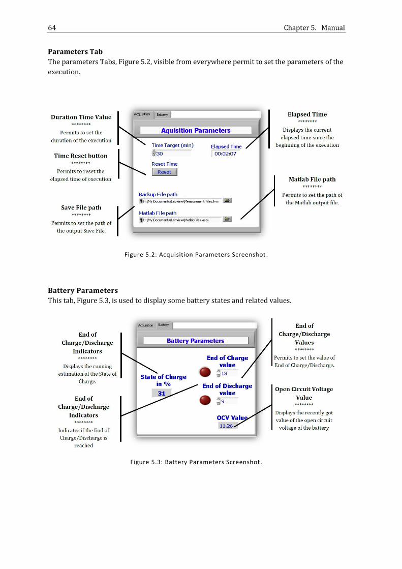
64 Chapter 5. Manual
Parameters Tab
The parameters Tabs, Figure 5.2, visible from everywhere permit to set the parameters of the
execution.
Figure 5.2: Acquisition Parameters Screenshot.
Battery Parameters
This tab, Figure 5.3, is used to display some battery states and related values.
Figure 5.3: Battery Parameters Screenshot.

5.4. Main Functions 65
5.4 MAIN FUNCTIONS
As visible in the previous paragraph, the Main Sections is composed of the principal functions
of the program. Each tab permits to define the parameters of the relating functions and to
display the corresponding outputs.
Graphs
This section displays 3 graphs, Figure 5.4, the general outputs of the system as the tension,
the current and the temperature of the battery pack.
Figure 5.4: Graphs Screenshot.
Charge
This section, Figure 5.5, permits to manage the charge of the battery by using the Constant
Charge method as well as the Pulse Modulation Charge method.
Figure 5.5: Charge Screenshot.

66 Chapter 5. Manual
Discharge
This section, Figure 5.6, allows to control the discharge values and also to display the
discharging current of the battery pack.
Figure 5.6: Discharge Screenshot.
Cell Balancing
This section, Figure 5.7 & 5.8, is the one of the balancing method allowing the balance of cells
during charge and discharges. The command can be set manually as well as automaticly by
using the Matlab script to generate it.
Figure 5.7: Cell Balancing Screenshot.

5.4. Main Functions 67
Figure 5.8: Cell Balancing Command Screenshot .
Simulation Tab
This section, Figure 5.9 permits to simulate some special and auto-executable experiments.
Figure 5.9: Simulation Tab Screenshot.

68 Chapter 5. Manual
The Capacity Test
This simulation tab, Figure 5.10, is used to show the values and state of the Capacity Test.
Figure 5.10: Capacity Test Screenshot.
The Step response
This simulation tab, Figure 5.11, is used to enter the timing values of the current step.
Figure 5.11: Step Response Screenshot.

5.4. Main Functions 69
Electrical Vehicle
This simulation tab, Figure 5.12, is used enter the timing values of the Electrical Vehicle
simulation.
Figure 5.12: Electrical Vehicle Screenshot.
General notes
If the program doesn’t stop, use the Run Execution bar to stop it
immediately. Be aware that stopping the program like that will leave the
hardware unchanged. Do not hesitate to shut down the power supply if
needed.
Sometimes during a run some commands are not available as the Enable
Charge/Discharge. In this case stop the program with the Run Execution
bar and run it again. It will most of the time solve the problems.
Do not forget to stop the program with the appropriate button on the
Front Panel to save the values of the experimentation in progress.
It’s recommended to disconnect the batteries if the bench is not used for a
long time, to prevent any problems related to the leaking current.

70
6 EXPERIMENTATIONS
This chapter will describe some experimental setups executed on the bench to highlight some
characteristics of the batteries or of the management.
6.1 INTRODUCTION
This chapter will describe some experimentation executed on the bench to highlight some
characteristics of the batteries or of the management. The experimentations below have been
chosen in order to used and test the program already implanted in the bench.
6.2 AUTO CELL BALANCING IMPROVEMENTS
The goal of this experimentation is to show the improvement of the Auto Balancing method
on the battery by executing Capacity tests.
In a first part, a capacity test is executed without Auto Balancing method. This Capacity test
will be the reference of capacity for a classic charge of the batteries.
Parameters
Time of Experimentation: 138 min
End of Charge value: 12 Volts
End of Discharge value: 10 Volts
Tension of Charge: 14 Volts
Current of Charge: 1.4 Amperes
Current of Discharge: 1.35 Amperes
On Figure 6.1, as the other Figures of the experimentation, the first curve corresponds to the
current values in the battery; the second curve shows the tension in the battery; and the third
curve highlights the tension in each cell of the battery pack.

6.2. Auto Cell Balancing Improvements 71
Capture
Figure 6.1: First Capacity Graph for Auto Cell Balancing Improvements.
Capacity Charged: 6048 A.s
In a second part, Figure 6.2, a second capacity test is launch this time with an Auto Balancing
method activated.
Figure 6.2: Second Capacity Graph for Auto Cell Balancing Improvements .
Capacity Charged: 11487 A.s
By the comparison of the 2 results, we observe and improvement of 90% of the capacity
charged, which makes in highlight the importance and the necessity of the Balancing Method
on the the battery cells.

72 Chapter 6. Experimentations
6.3 ELECTRICAL VEHICLE
The goal of this experimentation is to show how the behavior of an electrical vehicle could be
destructive for the batteries, and how the Auto Balancing could increase the range of the
batteries.
As saw in the section 4.6.3, during a defined period of time, the battery suffers the
accelerations and brakes of an Electrical Vehicle.
Parameters
Time of Experimentation: 89 min
End of Charge value: 12 Volts
End of Discharge value: 10 Volts
Tension of Charge: 14 Volts
Current of Charge: 1.4 Amperes
Sequence Timing
End of Brake: 15 sec
End of Acceleration Max: 60sec
End of Acceleration: 120 sec
End of Sequence: 600 sec
Figure 6.3 shows the experimentation repeated several times, at the end a capacity test is
executed to estimate the losses of capacity.
Figure 6.3: Electrical Vehicle Experimentation.

6.3. Electrical Vehicle 73
Figure 6.4 shows the capacity of the battery after the Electrical Vehicle experimentations.
Figure 6.4: Capacity after Electrical Vehicle Experimentation.
Capacity Charged: 4138 A.s
By the comparison of the 2 results, this makes in highlight the deterioration of the battery by
behavior of an electrical vehicle. The deterioration is about 31% of the capacity chargeable in
the battery.
The different simulations and experimentation that have been done, can lead to conclude that
the Lithium-Ion battery mus be managed differently to be used in the application of an
Electrical Vehicle. By assuming that the test bench is working properly, we see that just a
simulation as an EV during about 15 minutes, even if it was repeated several times, gave a
deterioration of the charge capacity of the battery up to 31%. Thus it is easy to understand
that using the li-ion battery during years is simply not possible due to its fast damage if used
as in the experimentation
.
74
7 CONCLUSION
7.1 CONCLUSION
During the Project, a test bench for a Battery Management has been designed. The design was
made to fulfill the main requirements found in the literatures, namely the objectives common
to all battery management system such as the protection of the cells, prolong the life of the
battery, and maintain the battery in a state in which it can fulfill the functional requirements
of the application for which it was specified. The choice of the battery was led by the potential
of it, and drove to choose the Lithium-Ion battery. At the end the BMS became fully
operational, assisted by the software Labview, which appeared obvious to use even though it
was very hard to understand it at the beginning. As required the cell balancing for 3 Li-Ion
cells, is working in manual or automatic mode. The safety requirements found in the
literatures were implemented, Even if the thermometer, it was working in good order, a
better accuracy could have been desired in to increase the safety of the BMS.
But the main conclusion that is possible to have is about the choice of the battery in a
particular utilization like an Electrical Vehicle. The experimentations have shown the
improvement of charge impacted by the balancing method, and confirmed the great
performance of the system itself in addition to show that the cell balancing is mandatory for
any Battery Management System. But on the other hand, the primary results have shown that
the Lithium-Ion battery must be well managed to be used in an EV, the short strong charges
and discharges given randomly have damaged the battery after only few repetitions.
7.2 FUTURE WORK
The next step for this project would be to implement everything on a Printed Circuit Board,
and confirm all the results gotten before. As the first wish was to be a test bench, and
compatible with the most common batteries used, another step could be to add a design
common to multiple batteries and not only the Li-Ion. Introduce the Kalman filter method,
with the help of Matlab, for the estimation of the State Of Charge seems to be a mandatory
task in a near future.
75
REFERENCES
[1] Amir Hossein Ranjbar, A. B. (n.d.). Online Estimation of State of Charge in Li-Ion Batteries
Using Impulse Response Concept. IEEE TRANSACTIONS ON SMART GRID, VOL. 3, NO. 1,
MARCH 2012.
[2] B. S. Bhangu, P. B. (n.d.). Nonlinear Observers for Predicting State-of-Charge and State-of-
Health of Lead-Acid Batteries for Hybrid-Electric Vehicles. IEEE TRANSACTIONS ON
VEHICULAR TECHNOLOGY.
[3] Bharath Pattipati, C. S. (n.d.). System Identification and Estimation Framework for Pivotal
Automotive Battery Management System Characteristics. IEEE TRANSACTIONS ON
SYSTEMS, MAN, AND CYBERNETICS—PART C: APPLICATIONS AND REVIEWS, VOL. 41,
NO. 6, NOVEMBER 2011.
[4] Cho, J. K. (n.d.). State-of-Charge Estimation and State-of-Health Prediction of a Li-Ion
Degraded Battery Based on an EKF Combined With a Per-Unit System. IEEE
TRANSACTIONS ON VEHICULAR TECHNOLOGY, VOL. 60, NO. 9, NOVEMBER 2011.
[5] Chow, H. Z.-Y. (n.d.). On-line PHEV Battery Hysteresis Effect Dynamics. Department of
Electrical and Computer Engineering, North Carolina State University, NC 27606 USA.
[6] Dongping XU, L. W. (n.d.). Research on Li-ion Battery Management System. Insititute of
Electrical Engineering Chinese Academy of Science, Beijing,China 100190.
[7] Fabio Codecà, S. M. (n.d.). The mix estimation algorithm for battery State-of-Charge
estimator – Analysis of the sensitivity to measurement errors. Joint 48th IEEE
Conference on Decision and Control and 28th Chinese Control Conference. Shanghai, P.R.
China, December 16-18, 2009.
[8] Jian Cao, N. S. (n.d.). Battery balancing methods: a comprehensive review. IEEE Vehicle
Power and propulsion conference (VPPC), Spetember 3-5,2008,Harbin,China.
[9] Martin Coleman, C. K. (n.d.). State-of-Charge Determination From EMF Voltage Estimation:
Using Impedance, Terminal Voltage, and Current for Lead-Acid and Lithium-Ion
Batteries. IEEE TRANSACTIONS ON INDUSTRIAL ELECTRONICS, VOL. 54, NO. 5,
OCTOBER 2007.
[10] Mohamed Daowd, N. O. (n.d.). Passive and Active Battery Balancing comparison based on
MATLAB Simulation.
[11] Peiying Li, Y. P. (2011). Study on an Active Voltage Equalization Charge System of a
Series Battery Pack.

76 References
[12] Seong-jun Lee, J.-h. K.-m.-h. (n.d.). The Estimation of the SOC and Capacity for the Lithium-
Ion Battery using Kalman Filter. School of Electrical Engineering and Computer
Science, Seoul National Univ. #043 San 56-1, Sillim-dong, Gwanak-ku, Seoul, 151-744,
Korea.
[13] Wang Haiying, H. L. (n.d.). Study on Correlation with SOH and EIS Model of Li-ion
Battery. 2011 The 6th International Forum on Strategic Technology.
[14] Li Siguang, (2009). Study on Battery Management System and Lithium-ion Battery. Sch.
of Mech. & Vehicular Eng., Beijing Inst. of Technol., Beijing, Computer and Automation
Engineering, 2009. ICCAE '09. International Conference.
[15] www.batteryuniversity.com
[16] www.batteryspace.com
[17] Aditya, J.P., 2008, Comparison of NiMH and Li-ion batteries in automotive applications,
Power Electron. & Motor Drives Lab., Missouri Univ. of Sci. & Technol., Rolla, MO.

77
NOTATIONS
AC: Alternate Current
ADC: Analogic to Digital Converter
BMS: Batteries Management System
DAQ: Data Acquisition
DC: Direct Current
EV: Electrical Vehicle
FET: Field Effect Transistor
FPGA: field-programmable gate array
GND: Ground
HEV: Hybrid Electrical Vehicle
IC: Integrated Circuit
OCV: Open Circuit Voltage
PMC: Pulse Modulation Charge
SOC: State of Charge
SOH: State of health

78
COMPONENTS USED
-Battery pack 3.6 V 2.3 Ah, H2B296
-Power transistor TO-220 NPN 100 V, BD
-Transistor TO-92 NPN 80 V 1 A, BC 639-16ZL1G
-Zener diode DO-35 glass 2.4 V 500 mW, BZX 55C2V4
-Comparator 4x DIL-14, LM339AN/NOPB
-Carbon potentiometer linear 10 kΩ ±20 %, STRK09K113
-Current transformer, 3...50 A, HX 03-P/SP2
-Voltage regulator 5 V TO-92, LM340LAZ-5.0/NOPB
-PCB power relay 12 VDC 530 mW, G2R-1A 12DC
-Charger, Li-polymer/Li-ion, 9C94017
-Temperature sensor TO-92, LM335AZ/NOPB
-Power resistor assortment 5 W ±10% E6/E12, CCR-32

Upphovsrätt/Copyright Svenska Detta dokument hålls tillgängligt på Internet - eller dess framtida ersättare - under en längre tid från publiceringsdatum under f¨orutsättning att inga extraordinära omständigheter uppstår. Tillgång till dokumentet innebär tillstånd för var och en att läsa, ladda ner, skriva ut enstaka kopior för enskilt bruk och att använda det oförändrat för ickekommersiell forskning och för undervisning. Överföring av upphovsrätten vid en senare tidpunkt kan inte upphäva detta tillstånd. All annan användning av dokumentet kräver upphovsmannens medgivande. För att garantera äktheten, säkerheten och tillgängligheten finns det l¨osningar av teknisk och administrative art. Upphovsmannens ideella rätt innefattar rätt att bli nämnd som upphovsman i den omfattning som god sed kräver vid användning av dokumentet på ovan beskrivna sätt samt skydd mot att dokumentet ändras eller presenteras i sådan form eller i sådant sammanhang som är kränkande för upphovsmannens litterära eller konstnärliga anseende eller egenart. För ytterligare information om Linköping University Electronic Press se förlagets hemsida: http://www.ep.liu.se/ English The publishers will keep this document online on the Internet - or its possible replacement - for a considerable time from the date of publication barring exceptional circumstances. The online availability of the document implies a permanent permission for anyone to read, to download, to print out single copies for your own use and to use it unchanged for any non-commercial research and educational purpose. Subsequent transfers of copyright cannot revoke this permission. All other uses of the document are conditional on the consent of the copyright owner. The publisher has taken technical and administrative measures to assure authenticity, security and accessibility. According to intellectual property law the author has the right to be mentioned when his/her work is accessed as described above and to be protected against infringement. For additional information about the Linköping University Electronic Press and its procedures for publication and for assurance of document integrity, please refer to its www home page: http://www.ep.liu.se/

© Johann Dussarrat Gael Balondrade Linköping, September 14, 2012