Design of a Rail-to-Rail Folded Cascode Amplifier with ... · Design of a Rail-to-Rail Folded...
4
1 Design of a Rail-to-Rail Folded Cascode Amplifier with Transconductance Feedback Circuit Radu Ciocoveanu, Andreas Bahr, and Wolfgang H. Krautschneider Abstract—In this work a programmable folded cascode rail- to-rail operational amplifier (OpAmp) with small settling time and transconductance feedback circuit is proposed. It employs a 130 nm CMOS technology with 1.2 V power supply. The small settling time is required to charge an ADC within a given time frame. The OpAmp achieves a gain bandwidth of 19.95 MHz with a 70 pF load and a minimum settling time of 144 ns while consuming 0.551 mA quiescent current. It can be shown that with 130 nm technology, high performance amplifiers can be realized on very small area. Index Terms—Small settling time, constant transconductance, rail-to-rail, programmable, operational amplifier. I. I NTRODUCTION T HE downscaling of the technology has led to lower supply voltages, in order to maintain a constant electric field. With a lower supply voltage, the signal-to-noise ratio has also decreased. To counteract this drawback, it is necessary to make use of the entire signal swing, thus rail-to-rail operation at both the input and output is needed. Rail-to-rail at the input can be achieved by using com- plementary n-channel and p-channel differential pair, but the drawback is that the g m is varying over the input common mode range, which leads to introduction of distortions, im- pedes optimal frequency compensation and also leads to a variation of GBW [1]-[3]. Additional circuitry is needed to maintain the g m constant over the input common mode range. In this work, a programmable rail-to-rail folded cascode amplifier in 130 nm technology with 1.2 V power supply voltage using the topology of [1] is presented, along with the feedback module to maintain the g m constant, with the topology shown in [2]. II. OPAMP AND FEEDBACK MODULE ARCHITECTURE A. Overall Architecture The programmable amplifier is used in a non-inverting configuration. A resistor string and transmission gates are added to allow the selection of different amplification values. The complete schematic of the programmable OpAmp is shown in Fig. 1. Vinp Vinn Vbn Vout Vbp Iab Vinp Vinn ΔV Ifb Vbp Vbn Vinp Vinn Vout Vinn VDD Vinp Vout ΔV Vbp Vbn Ifb Iab 40k 20k 10k 10k Vinp Vref Gain<0> Gain<1> Gain<2> Gain<3> Feedback Module OpAmp Fig. 1. Complete schematic of the programmable OpAmp. The inputs of feedback module and folded cascode OpAmp are shared, and the voltages V bn and V bp adjust the currents through the input differential pair of the OpAmp, as it is shown in Fig. 1. ΔV is a DC voltage that causes an imbalance in the feedback module, which will lead to the generation of the two control voltages V bn and V bp . B. Folded Cascode OpAmp The schematic of the OpAmp is shown in Fig. 2. It has complementary p-channel and n-channel differential pairs to achieve rail-to-rail common mode voltage at the input (transis- tors MN01, MN02, MP01, MP02), and a class AB output stage to obtain rail-to-rail at the output of the amplifier (transistors MNAB, MPAB), as presented in [1]. Transistors MN03, MP03 are biasing the input differential pair, while transistors MP04, MP05, MP06, MP07 and MN04, MN05, MN06, MN07 are used in the cascode current mirrors. Transistors MP11, MP12 and MN11, MN12 represent the floating current source, which biases both the summing circuit and the class-AB control. Transistors MP09, MP10 and MN09, MN10 bias the gates of the transistors from the floating current source. The current source provides power-supply independent
Transcript of Design of a Rail-to-Rail Folded Cascode Amplifier with ... · Design of a Rail-to-Rail Folded...

1
Design of a Rail-to-Rail Folded Cascode Amplifierwith Transconductance Feedback Circuit
Radu Ciocoveanu, Andreas Bahr, and Wolfgang H. Krautschneider
Abstract—In this work a programmable folded cascode rail-to-rail operational amplifier (OpAmp) with small settling timeand transconductance feedback circuit is proposed. It employs a130 nm CMOS technology with 1.2 V power supply. The smallsettling time is required to charge an ADC within a given timeframe. The OpAmp achieves a gain bandwidth of 19.95 MHzwith a 70 pF load and a minimum settling time of 144 ns whileconsuming 0.551 mA quiescent current. It can be shown that with130 nm technology, high performance amplifiers can be realizedon very small area.
Index Terms—Small settling time, constant transconductance,rail-to-rail, programmable, operational amplifier.
I. INTRODUCTION
THE downscaling of the technology has led to lowersupply voltages, in order to maintain a constant electric
field. With a lower supply voltage, the signal-to-noise ratio hasalso decreased. To counteract this drawback, it is necessary tomake use of the entire signal swing, thus rail-to-rail operationat both the input and output is needed.
Rail-to-rail at the input can be achieved by using com-plementary n-channel and p-channel differential pair, but thedrawback is that the gm is varying over the input commonmode range, which leads to introduction of distortions, im-pedes optimal frequency compensation and also leads to avariation of GBW [1]-[3]. Additional circuitry is needed tomaintain the gm constant over the input common mode range.
In this work, a programmable rail-to-rail folded cascodeamplifier in 130 nm technology with 1.2 V power supplyvoltage using the topology of [1] is presented, along withthe feedback module to maintain the gm constant, with thetopology shown in [2].
II. OPAMP AND FEEDBACK MODULE ARCHITECTURE
A. Overall Architecture
The programmable amplifier is used in a non-invertingconfiguration. A resistor string and transmission gates areadded to allow the selection of different amplification values.The complete schematic of the programmable OpAmp isshown in Fig. 1.
Vinp
Vinn
Vbn
Vout
Vbp
Iab
Vinp
VinnΔV
IfbVbp
Vbn
Vinp
Vinn
Vout
Vinn
VDD
Vinp
VoutΔV
Vbp
Vbn
Ifb
Iab
40k
20k
10k
10k
Vinp
Vref
Gain<0>
Gain<1>
Gain<2>
Gain<3>
Feedback Module
OpAmp
Fig. 1. Complete schematic of the programmable OpAmp.
The inputs of feedback module and folded cascode OpAmpare shared, and the voltages Vbn and Vbp adjust the currentsthrough the input differential pair of the OpAmp, as it is shownin Fig. 1. ∆V is a DC voltage that causes an imbalance inthe feedback module, which will lead to the generation of thetwo control voltages Vbn and Vbp.
B. Folded Cascode OpAmp
The schematic of the OpAmp is shown in Fig. 2. It hascomplementary p-channel and n-channel differential pairs toachieve rail-to-rail common mode voltage at the input (transis-tors MN01, MN02, MP01, MP02), and a class AB output stageto obtain rail-to-rail at the output of the amplifier (transistorsMNAB, MPAB), as presented in [1].
Transistors MN03, MP03 are biasing the input differentialpair, while transistors MP04, MP05, MP06, MP07 and MN04,MN05, MN06, MN07 are used in the cascode current mirrors.Transistors MP11, MP12 and MN11, MN12 represent thefloating current source, which biases both the summing circuitand the class-AB control. Transistors MP09, MP10 and MN09,MN10 bias the gates of the transistors from the floating currentsource. The current source provides power-supply independent

2
quiescent current [1]. In a folded cascode without a floatingcurrent source, the current in the summation stage is varyingwith the common mode voltage at the input, which will causea change in the voltage that biases the gates of the outputtransistors, which in turn contributes to the noise and offset ofthe amplifier. The floating architecture of the class-AB driverprevents that it contributes to the noise and the offset of theamplifier [1]. Cascoded Miller compensation is used in orderto make the operational amplifier stable.
MN04
MN02
MP01 MP02
MN03
MP03MP04 MP05
MP06 MP07
MN05
MN06 MN07
MPAB
MNAB
C_Miller
MN01
C_Miller
Vbp
Vinp
Vout
Iab
Iab
VDD
MP09
MP10
MP11 MP12
MN11 MN12
MN10
MN09
Vbn
Vinn
In
2Ip
Isum Isum
In
Ip Ip Iout
Isum Isum
2In
Vbcp
Vbcn
Res
Res
Fig. 2. Proposed rail-to-rail amplifier [1].
The transconductance of the input stage is defined as
gmT = gMN01 + gMP01 (1)
and it varies by a factor of two over the input common moderange [3]. The variation can be explained as following: whenthe input common mode is VDD/2, both the NMOS and thePMOS transistors operate, therefore the transconductance is atits maximum in that region. At GND, the NMOS will turn offwhile the PMOS is still conducting. Because only the PMOSis conducting, the transconductance is half of what it is atVDD/2. At VDD, the PMOS is turned off, while the NMOSis turned on, therefore the transconductance is half of what itis at VDD/2. To keep the transconductance constant over theinput common mode range additional circuitry is needed.
C. Feedback Module
To maintain a constant gmT , the circuit schematic in Fig. 5is used, as presented in [2]. The functioning principle of thefeedback module is shown in Fig. 3.
+
-
+
-
VDD
2Ip
2In
ΔVΔi1 Δi2
ΔV
Vbp
Vbn
Feedback Module
MN02
MP01 MP02
MN01 VinpVinn
In In
Summation
Stage
+
Output
Stage
VDD
Ip Ip
2Ip
2In
Rail-to-Rail Input Stage
Vbp
Vbn
T1 T2
MN03
MP03
Fig. 3. Feedback module functioning principle [2].
The blocs T1 and T2 are transconductance amplifiers andtheir transconductance values are kept equal by the negativefeedback. The outputs of the feedback module are two controlvoltages Vbn and Vbp that adjust the currents through transis-tors MN03, MP03 [2]. Depending on the input common-mode,the two control voltages will make the transistors MN03 andMP03 conduct more or less current. The bloc T1 in Fig. 3 is thegmT −R converter and the bloc T2 is the resistive comparator.
The gmT −R converter is shown in Fig. 4. The transconduc-tance of the input stage gmT can be expressed as a function ofthe equivalent small signal resistance req,AB at nodes A andB [2].
req,AB =2
gmT + gds,NMOS + gds,PMOS[2] (2)
A B
VDD
2Ip
2In
Fig. 4. gmT −R converter [2].
The complete feedback module in Fig. 5 includes a dynamicbias generator that is used to provide a current (Ibias+In−Ip)for the two current sources MS1 and MS2. It also consistsof blocs T1 (gmT − R converter), T2 (resistive comparator)and a folded cascode transimpedance amplifier structure usedas current summation stage. T1 and T2 are unbalanced by aDC input voltage ∆V and generate two output currents. In thecurrent summation stage, the summation of currents from T1
and T2 is converted in the two controlling voltages Vbn andVbp that adjust the tail current sources in both the feedbackmodule and OpAmp [2].
The summation stage in Fig. 5 is a resistive comparator for(gmT +gds,NMOS +gds,PMOS)−1 and Rref . The tail currentswill be adjusted until (gmT + gds,NMOS + gds,PMOS)−1 =Rref [2].
Because gds,NMOS and gds,PMOS are small in comparisonto gmT , they can be ignored, therefore the equation becomes:
gmT = R−1ref = R−1
1 = R−12 [2] (3)
Two other important conditions have to be met for a goodfunctionality of the feedback module. The minimum value forthe reference resistance Rref is given by eq. 4.
Rref,min =1
gmf[2] (4)
3
Vinp Vinn Vinp Vinn
MN09 MN10 MP09 MP10
MP12 MP13 MP11 MP14MP15 MP16
Vb1 MP17 MS1 MS2
MS3 MS4
MP21 MP22
R1 R2D C
MP23
MP24
Vb1
Vb2
Vb3
Cc
Vbp
MN11 MN14 MN12 MN13 MN15 MN16 MN17
MN18
MN19 MN20
MP19 MP20
MP26 MP27 MP29 MP28
ΔV ΔV
MP18
MN21 MN22
MN23 MN24
MP25
MN25
Vbn
VDD
2In
4 : 1
4 : 1
In/2 2Ip Ip/2
1 : 4
1 : 1
(Ibias+In)/2 (Ibias+In-Ip)/2
Ibias+In-Ip Ibias+In-Ip
In/2 Ibias/2 1 : 2
4 : 1 2In
Ibias Ibias
PA B
1 : 1
1 : 41 : 1
Dynamic Bias Current Generator T1 T2 Current Summation Stage
2Ip
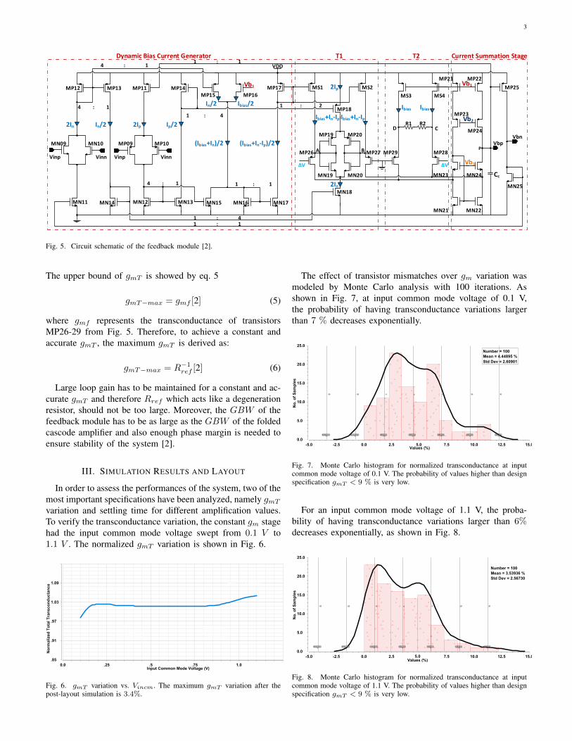
Fig. 5. Circuit schematic of the feedback module [2].
The upper bound of gmT is showed by eq. 5
gmT−max = gmf [2] (5)
where gmf represents the transconductance of transistorsMP26-29 from Fig. 5. Therefore, to achieve a constant andaccurate gmT , the maximum gmT is derived as:
gmT−max = R−1ref [2] (6)
Large loop gain has to be maintained for a constant and ac-curate gmT and therefore Rref which acts like a degenerationresistor, should not be too large. Moreover, the GBW of thefeedback module has to be as large as the GBW of the foldedcascode amplifier and also enough phase margin is needed toensure stability of the system [2].
III. SIMULATION RESULTS AND LAYOUT
In order to assess the performances of the system, two of themost important specifications have been analyzed, namely gmT
variation and settling time for different amplification values.To verify the transconductance variation, the constant gm stagehad the input common mode voltage swept from 0.1 V to1.1 V . The normalized gmT variation is shown in Fig. 6.
M14: 100.0m 982.5156m
M15: 1.1 1.049334
Nor
mal
ized
Tot
al T
rans
cond
ucta
nce
.85
.91
.97
1.03
1.09
Input Common Mode Voltage (V)0.0 .25 .5 .75 1.0
dx: 500.0mdy: 34.96805m s: 69.93611m/
dx: 500.0mdy: 31.85031m s: 63.70061m/
Fig. 6. gmT variation vs. Vincm. The maximum gmT variation after thepost-layout simulation is 3.4%.
The effect of transistor mismatches over gm variation wasmodeled by Monte Carlo analysis with 100 iterations. Asshown in Fig. 7, at input common mode voltage of 0.1 V,the probability of having transconductance variations largerthan 7 % decreases exponentially.
μ
4.44895
-σ
1.83993
σ
7.05796
-2σ
-769.078m
2σ
9.66697
-3σ
-3.37809
3σ
12.2760
No
. of
Sam
ple
s
0.0
5.0
10.0
15.0
20.0
25.0
5.0 -5.0 -2.5 0.0 2.5 7.5 10.0 12.5 15.0
Number = 100 Mean = 4.44895 %Std Dev = 2.60901
Values (%)
Fig. 7. Monte Carlo histogram for normalized transconductance at inputcommon mode voltage of 0.1 V. The probability of values higher than designspecification gmT < 9 % is very low.
For an input common mode voltage of 1.1 V, the proba-bility of having transconductance variations larger than 6%decreases exponentially, as shown in Fig. 8.
μ
3.53936
-σ
972.063m
σ
6.10666
-2σ
-1.59523
2σ
8.67396
-3σ
-4.16253
3σ
11.2413
No
. of
Sam
ple
s
0.0
5.0
10.0
15.0
20.0
25.0
5.0 Values (%)
-5.0 -2.5 0.0 2.5 7.5 10.0 12.5 15.0
Number = 100 Mean = 3.53936 % Std Dev = 2.56730
Fig. 8. Monte Carlo histogram for normalized transconductance at inputcommon mode voltage of 1.1 V. The probability of values higher than designspecification gmT < 9 % is very low.

4
Settling time is a critical specification for this design,because the amplifier has to settle to 1/2 LSB within a giventime frame, in order for the ADC to sample the value correctly.
To measure the settling time, a probe was first added at themoment when the pulse is applied at the input, and a secondprobe, when the output value of the amplifier is within 1/2LSB of the final value and time difference between the twowas measured.
V (
V)
-.25
0.0
.25
.5
.75
1.0
time (us)12.5 15.0 17.5 20.0 22.5 25.0
Fig. 9. Settling time simulation.
The values for the settling time for the different amplifica-tion factors are given in table I.
Amplification Value Rise Time Fall Time
1 144 ns 329 ns 2 490 ns 491 ns 4 308 ns 482.95 ns 8 387 ns 484.13 ns
TABLE ISIMULATED SETTLING TIME FOR DIFFERENT AMPLIFICATION FACTORS.
The area consumption of the layout in Fig. 10 is only0.0231 mm2.
117 µm
197.6 µm
Feedback Module
Miller Compensation
Folded-Cascode
Feedback Resistors
and Switches
Fig. 10. Layout of the complete rail-to-rail OpAmp with transconductancefeedback module.
IV. CONCLUSION
The performance comparison of the rail-to-rail amplifier issummarized in table II, showing a lower power consumptionthan in [4] as well as a smaller settling time, larger slew rateand less area consumption.
[3] [2] This paper
Process 0.13 µm 0.13 µm 0.13 µm
Supply Voltage (V) 1.2 1 1.2
Maximum gmT variation
13 % 3.4 % 3.4 %
Load 70 pF 20 kΩ || 95 pF 70 pF
DC Gain (dB) 85 60 71.6
Power Consumption (mW)
1.28 0.187* 0.662
GBW (MHz) 4.99 3.7 19.95
Phase Margin 67° 72° 64°
Slew Rate (V/µs) 0.9 1.74 7.39
Minimum Settling Time (µs)
≈ 0.464** - 0.144
Occupied area (mm2)
0.109 mm2 0.0289 mm2 0.0231 mm2
* Only the power-consumption of folded-cascode amplifier is considered. ** Minimum settling-time achieved for the specified power consumption. In [4], the power consumption is 1.28 mW .
TABLE IIPERFORMANCE COMPARISON.
This paper has presented a programmable rail-to-rail am-plifier with transconductance feedback technique, with smallsettling time and good constant transconductance over theinput common mode range. The simulated results show goodperformance of the amplifier, with low power consumption,large slew rate and small occupied area.
V. ACKNOWLEDGEMENTS
This work was supported by the German Research Founda-tion, Priority Program SPP1665.
REFERENCES
[1] R. Hogervorst, J. P. Tero, R. Eschauzier, and P. W. Daly, ”A compactpower-efficient 3 V CMOS rail-to-rail input/output operational amplifierfor VLSI cell libraries”, IEEE J. Solid-State Circuits vol. 29, no. 12,pp. 15051513, 1994.
[2] S. Dai, X. Cao, T. Yi, E. Hubbard, and Z. Hong, ”1-V Low-Power Pro-grammable Rail-to-Rail Operational Amplifier With Improved Transcon-ductance Feedback Technique”, IEEE Trans. VLSI Syst vol. 21, no. 10,pp. 19281935, 2013.
[3] Willy M. C. Sansen, Analog Design Essentials,Dordrecht: Springer, 2006, ISBN: 978-0-387-25747-1, URL:http://www.springer.com/gb/1850-9999.
[4] J. M. Tomasik, K. M. Hafkemeyer, W. Galjan, D. Schroeder, andW. H. Krautschneider, ”A 130nm CMOS Programmable OperationalAmplifier”, in 2008 NORCHIP pp. 2932.


![Cascode Switching Modeling and Improvement in Flyback ...Cascode GaN FET [10], during inductive hard switching. Figure 2 Cascode Switching Configured Flyback converter II. MODELING](https://static.fdocuments.net/doc/165x107/5e541119f61a9f6e2b2e813c/cascode-switching-modeling-and-improvement-in-flyback-cascode-gan-fet-10.jpg)