Design of a Mobile Coastal Communications Buoy

By

Meghan Hendry-Brogan

B.S., Ocean Engineering (2003)

Massachusetts Institute of Technology

Submitted to the Department of Ocean Engineering in Partial Fulfillment of the Requirements for the Degree of

Master of Science in Naval Architecture and Marine Engineering

at the

Massachusetts Institute of Technology

September 2004

© Massachusetts Institute of Technology All rights reserved

Signature of Author ………………………………………………………………………..

Department of Ocean Engineering August 6, 2004

Certified by ………………………………………………………………………………...

Chrysosstomos Chrysosstomidis Henry L. and Grace Doherty Professor of Ocean Science and Engineering

Thesis Supervisor

Accepted by ……………………………………………………………………………….. Michael Triantafyllou

Professor of Ocean Engineering Chairman, Department Committee on Graduate Studies

1

Design of a Mobile Coastal Communications Buoy

by

Meghan Hendry-Brogan

Submitted to the Department of Ocean Engineering on August 6, 2004 in partial fulfillment of the requirements

for the degree of Master of Science in Naval Architecture and Marine Engineering

Abstract In response to a growing interest in networked communications at sea as well as the needs of our vital commercial fishing industry, the Northeast Consortium funded a novel research initiative to establish wireless acoustic and radio communications at sea. The platform used for this type of telemetry instrumentation was to be a buoy which could not only withstand the often harsh conditions off the northeastern coast of America (specifically, Cape Ann), but do so while exhibiting an exceptionally small response in heave and roll.

A spar type buoy was designed and built at the MIT Sea Grant facility. Spars are a special type of buoy shape whose hydrostatic and hydrodynamic interactions with the sea are decoupled enough so that extreme sea conditions do not induce extreme buoy motions. Most oceanographic buoys are of the discus type, and move as the surface of the ocean does. This type of wave-following buoy would not sufficiently facilitate the requirements of the high-bandwidth wireless networking hardware, and therefore would not serve the current purpose.

The NEC buoy displaces approximately 140 kg of sea water and is roughly 11 feet long when fully assembled, not including its 5 foot antenna mast. The buoy employs a PC104 stack to control an 802.11b wireless card and antenna, an acoustic modem card and transducer, other peripheral instrumentation, a main battery, and a solar power system. Thesis Supervisor: Chryssostomos Chryssostomidis Title: Henry L and Grace Doherty Professor of Ocean Science and Engineering

2

Biographical Note and Acknowledgements

Meghan Hendry-Brogan graduated with her Bachelors of Science in Ocean Engineering from the Massachusetts Institute of Technology in June of 2003. At MIT she was an officer in the 13Seas student group which implies membership to the Society of Naval Architecture and Marine Engineering and the Marine Technology Society. She played varsity volleyball, basketball, ran track and sailed during her undergraduate years. She also spent every summer in a different industrial internship. Having been awarded one of the National Defense Science and Engineering Fellowships funded by the Office of Naval Research, she reentered MIT in the fall of 2003 to work on a Masters of Science degree in Naval Architecture and Marine Engineering. She has truly enjoyed every second she spent at the Institute and is very grateful to God and everyone who made that possible.

Meghan harbors a deep love for the marine environment due largely to being raised on the beaches of South Florida. Most of her childhood and adolescence was centered on daily trips to the beach, fishing or boating in the intercoastal waterway, diving and snorkeling. Anyone who has spent any part of their life in the coastal cities of Florida knows what kind of lifestyle that implies. Meghan has accepted a job next year in the Offshore Oil and Gas Industry in Houston, TX.

The NEC Buoy research was made possible primarily by Professor Chryssostomidis and the Northeast Consortium (Grant #NA03NMF4720205). Professor Chryssostomidis and his right-hand-women, Rere and Kathy, have been a constant source of help and encouragement since I affiliated myself with the MIT Ocean Engineering department five years ago. The research engineers in the AUV Lab were of course invaluable, as they are to almost every project that works its way through MIT Sea Grant. I am very grateful to Sam Desset, Jim Morash, Vic Polidoro, and Rob Damus for the hours of excruciating pain spent in lab meetings. I am grateful to God for giving those four men such large quantities of both intelligence and patience, especially Sam who completely annihilated my belligerent belief that nothing good ever came from France. To my office mate and now friend, Costa, free is not dead; any time you need a place to stay in Texas, Florida, or any of those other wonderful and perfect southern states just call me. To my Grammy Hendry and all my aunts, uncles and cousins here in Massachusetts who have given me places to stay, warm meals, clean cloths, and lots of love and support I owe you all so much. Mom, Dad, David and Sean, what can I say? You all are the reason I exist, and in many ways I have come this far both because of you and for you. I love you.

3

1. INTRODUCTION ............................................................................................................................. 7

1.1 RESEARCH OBJECTIVES...................................................................................................................... 7 1.1.1 General ...................................................................................................................................... 7 1.1.2 Personal ..................................................................................................................................... 8

1.2 MOTIVATION....................................................................................................................................... 8 1.2.1 The NEC.................................................................................................................................... 8 1.2.2 Traditional Sensors ................................................................................................................... 9 1.2.3 Navigation and Position............................................................................................................ 9

1.3 BACKGROUND INFORMATION............................................................................................................. 9 1.3.1 Networked, Autonomous Ocean Communication....................................................................... 9 1.3.2 History of Buoys...................................................................................................................... 10 1.3.3 WAN........................................................................................................................................ 11

1.4 PROJECT MANAGEMENT ................................................................................................................... 11 1.4.1 Schedule and Budget............................................................................................................... 12

1.5 BUOY OPTIONS .................................................................................................................................. 12 1.5.1 Others out there? .................................................................................................................... 14 1.5.2 Spar characteristics and justification ..................................................................................... 15

2. ENVIRONMENTAL DESIGN CRITERIA.................................................................................. 17 2.1 NORTH ATLANTIC ............................................................................................................................ 17

2.1.1 Wave Data................................................................................................................................ 17 2.1.2 Current and Tide Data............................................................................................................. 20

2.2 ALTERNATIVE OPERATING ENVIRONMENTS..................................................................................... 21 2.3 FINAL SEA STATE MODEL ................................................................................................................ 22 2.4 WAVE STATISTICS............................................................................................................................ 22

2.4.1 Spectral Analysis...................................................................................................................... 23 2.4.2 Short term................................................................................................................................. 24

3. NEC BUOY DESIGN AND ANALYSIS ....................................................................................... 26 3.1 DESIGN OVERVIEW ........................................................................................................................... 26

3.1.1 Scale and Dimension................................................................................................................ 26 3.1.2 Design Process........................................................................................................................ 26 3.1.3 Weight Estimate ...................................................................................................................... 30 3.1.4 Basic Statics ............................................................................................................................ 31

3.2 DYNAMICS ........................................................................................................................................ 32 3.2.1 Hydrodynamic Loading............................................................................................................ 33 3.2.2 Heave Analysis........................................................................................................................ 33 3.2.3 Roll Analysis ........................................................................................................................... 40 3.2.4 Developing Seas Issue............................................................................................................. 46

3.3 MOORING DESIGN ............................................................................................................................. 46 3.3.1 Line Dynamics ......................................................................................................................... 47 3.3.2 Matlab Simulation.................................................................................................................... 48

3.4 STRUCTURAL DESIGN ....................................................................................................................... 51 3.4.1 Materials .................................................................................................................................. 52 3.4.2 COSMOS Analysis ................................................................................................................... 52

3.5 ELECTRONIC SYSTEMS OUTLINE....................................................................................................... 54 3.5.1 Power System ........................................................................................................................... 55 3.5.2 WHOI Micro-Modem ............................................................................................................... 57 3.5.3 Computer ................................................................................................................................. 58 3.5.4 Hardware ................................................................................................................................. 58

3.6 COMMUNICATIONS SOFTWARE OVERVIEW ....................................................................................... 58

4

4. NEC BUOY TESTING.................................................................................................................... 60

4.1 OBJECTIVES ...................................................................................................................................... 60 4.1.1 Short Term ............................................................................................................................... 60 4.1.2 Long Term................................................................................................................................ 60

4.2 TESTING PHASES ............................................................................................................................... 61 4.2.1 Phase I ..................................................................................................................................... 61 4.2.2 Phases II .................................................................................................................................. 63 4.2.3 Phase III................................................................................................................................... 63 4.2.4 Phase IV................................................................................................................................... 63

4.3 TEST VARIABLES .............................................................................................................................. 63 4.3.1 Message Type........................................................................................................................... 64

5. MOBILE GIB BUOY DESIGN...................................................................................................... 65 5.1 EXISTING MODEL.............................................................................................................................. 65 5.2 POTENTIAL DESIGNS ......................................................................................................................... 66

5.2.1 SWATH Type............................................................................................................................ 66 5.2.2 Other Ideas............................................................................................................................... 67

5.3 EVALUATION AND RECOMMENDATIONS ........................................................................................... 68 6. CONCLUSIONS.............................................................................................................................. 69

6.1 MEASURE OF SUCCESS ...................................................................................................................... 69 6.2 FUTURE WORK.................................................................................................................................. 69

7. REFERENCES ................................................................................................................................ 71 8. APPENDICES.................................................................................................................................. 73

8.1 APPENDIX 1: HEAVE DYNAMICS MATLAB SCRIPT ............................................................................ 73 8.2 APPENDIX 2: ROLL DYNAMICS MATLAB SCRIPT............................................................................... 76 8.3 APPENDIX 3: MOORING WEIGHT ESTIMATE...................................................................................... 79

5

List of Figures: Figure 1. NDBC "NOMAD" Buoy [25] ...................................................................................................... 13 Figure 2. a) Discus Buoy b) Spar Buoy c) DDCV Hoover Diana ............................................................... 13 Figure 3. Data Buoy Map [17]..................................................................................................................... 18 Figure 4. Wave Height Histogram for 44029 .............................................................................................. 18 Figure 5. Sea State Histogram for GoMOOS Buoy 44029.......................................................................... 19 Figure 6. Sea State Histogram for NOAA Buoy 44013............................................................................... 19 Figure 7. Mass Bay Buoy 44029 Current Measurements [17] .................................................................... 20 Figure 8. Mass Bay Buoy 44029 Current Profile ........................................................................................ 21 Figure 9. Bretschneider Model .................................................................................................................... 22 Figure 10. Foam Buoy Design..................................................................................................................... 28 Figure 11. Phase II Design Considerations.................................................................................................. 29 Figure 12. Final NEC Buoy Design............................................................................................................. 30 Figure 13. Heave Analysis Diagram............................................................................................................ 34 Figure 14. Actual Heave Forcing Terms ..................................................................................................... 36 Figure 15. Idealized Heave Transfer Function ............................................................................................ 37 Figure 16. Actual Heave Transfer Function for the Final Design ............................................................... 38 Figure 17. Heave Response Spectrum [m] .................................................................................................. 39 Figure 18. Heave Velocity and Acceleration Spectra.................................................................................. 39 Figure 19. Parametric Heave Analysis ........................................................................................................ 40 Figure 20. Roll Body Diagram .................................................................................................................... 41 Figure 21. Roll Coefficients ........................................................................................................................ 43 Figure 22. Actual Roll Transfer Function for the Final Design................................................................... 44 Figure 23. Roll Response Spectrum [m]...................................................................................................... 45 Figure 24. Roll Velocity and Acceleration Spectra ..................................................................................... 45 Figure 25. Representative Developing Sea Spectra..................................................................................... 46 Figure 26. Line Segment Definition ............................................................................................................ 48 Figure 27. Reynolds Number for the Given Current Profile and 5/8” Line................................................. 49 Figure 28. Buoy and Mooring Offset for L/H ratio 1.3 with Polypropylene Line....................................... 50 Figure 29. Buoy and Mooring Offset for L/H Ratio 2.4 and Nylon Line.................................................... 50 Figure 30. Stress and Deformation Plots for Load Case #1......................................................................... 53 Figure 31. NEC Buoy System Schematic.................................................................................................... 55 Figure 32. Software Hierarchy .................................................................................................................... 59 Figure 34. Buoy Assembly: Section 2 Attached.......................................................................................... 62 Figure 35. Buoy Testing Environment ........................................................................................................ 62 Figure 36. Mobile GIB Concept, BASIL [24] Figure 37. MiniVAMP Vehicle [24]................ 65 Figure 38. SWATH Concept ....................................................................................................................... 66 Figure 39. SWATH-type Mobile Comms Buoy.......................................................................................... 67

List of Tables: Table 1. Data Buoy Definitions................................................................................................................... 18 Table 2. Sea State Definition [26] ............................................................................................................... 19 Table 3. Wave Statistics .............................................................................................................................. 25 Table 4. Buoy Dimensions .......................................................................................................................... 30 Table 5. NEC Buoy Weight Estimate.......................................................................................................... 31 Table 6. NEC Buoy Hydrostatic Characteristics ......................................................................................... 31 Table 7. Heave Predictions.......................................................................................................................... 39 Table 8. Predicted Communication Efficiencies [8].................................................................................... 41 Table 9. Roll Predictions ............................................................................................................................. 45 Table 10. Mooring Simulation Models and Results .................................................................................... 51 Table 11. Buoy Material Properties............................................................................................................. 52 Table 12. Load Case #1 Results .................................................................................................................. 53 Table 13. Load Case #2 Results .................................................................................................................. 53 Table 14. Power Consumption by Instrument ............................................................................................. 56

6

1. Introduction The research engineers at MIT Sea Grant successfully submitted a grant proposal

to a research program called the Northeast Consortium in the FY-2003. Accompanying the award of this grant were the requirements that a communications buoy be constructed for operation in the near shore areas off of Cape Ann. This buoy was to have the ability to communicate with a land based antenna and establish a wireless area network (WAN) in its immediate vicinity (~3nm radius). The general description of this goal is for fisherman to be able to download vital information off the World Wide Web from their vessels and at much higher data transfer rates than those afforded by existing means. All they would need to be able to do is locate the buoy and position themselves within the WAN.

This may, at first, not seem like such a novel or ambitious goal given that technologies such as ARGOS and INMARSAT have existed for years. For that reason it is important to outline the fundamental differences between these competing technologies and show why this current research is useful. Both ARGOS and INMARSAT are expensive and slow. Both of those disadvantages largely take root in the fact that the information must be passed through a satellite on rented time. Reliability is a third issue at the heart of the comparison. While one buoy may not be more consistently available than a satellite, a network of buoys with redundant communications paths to shore certainly is. This work is helping to push the boundaries of our current capabilities by helping to take effective communications techniques to the sea.

Along with the differentiating ability to establish a WAN, this communications buoy would of course need to be able to do all of the things a generic ocean-data buoy is able to do. Addressing the naval architectural focus of this thesis and its associated degree, the buoy must be adequately designed for its environment, behave in a fully analyzed and generally predictable manner, be accompanied by a mooring system which is also understood, and be (provably) structurally sound.

1.1 Research Objectives

1.1.1 General The generalized objectives of this research are listed here. They are derived from

the stated goals of the funding agency, the Northeast Consortium, and the direction of the fields of naval architecture and marine engineering as a whole.

1. Design a 100-200kg buoy to provide radio and acoustic telemetry to local (surface and underwater) vessels, and act as an information pass-through

2. Build and demonstrate the ability of a prototype buoy to meet those demands while surviving up to a Sea State 4 condition

3. Explore the technical feasibility of mid-range spar buoy applications for communications missions

4. Assess the feasibility of taking the communications buoy idea one step farther and making it autonomously or remotely mobile

7

The motivation for these goals lies largely in the idea that adding to the base of knowledge we already have regarding communications at sea is desirable. The field of wireless, networked communication is being studied intensely in general, and is much farther along in the land-based applications. Additionally, on the naval architectural side, observations of existing spar buoys for scientific or communications applications show that the majority of systems are for one of two scales: small and lightweight (15-30 kg displacement) or very-large and high-budget (1,000+ kg displacement). Exploring the feasibility of using a spar buoy in the 100-150kg displacement range for a communications mission scenario is both novel and interesting.

1.1.2 Personal The type of buoy design which has been prescribed by this particular thesis and

the accompanying research is in some ways microcosmic of, and in other ways directly scalable to, those projects which are undertaken by naval architects and marine engineers who work to design large scale systems for the open ocean. The offshore engineer designing a tension leg platform, Deep Draft Caisson Vessel (DDCV), or most similarly, a single point moored oil offloading buoy for 7000 feet of water follows roughly the same design path as was required for this communications buoy. Because I, the researcher, hope to matriculate into the offshore engineering industry, I can only benefit from the completion of the stated research. I personally, hope to ameliorate my project management and design skills such that I will be able to contribute more in my future career.

1.2 Motivation

1.2.1 The NEC The Northeast Consortium (NEC), likened to the ‘client’ in a real world design environment, was created in 1999 to encourage and fund partnerships between commercial fisherman and the researchers working to aid their trade. The Consortium is comprised of representatives from the University of New Hampshire, the Woods Hole Oceanographic Institution, the University of Maine, and the Massachusetts Institute of Technology. The research which they support is meant to focus on the Gulf of Maine and Georges Bank fishing areas. In 2002, the NEC had approximately $5 Million to fund those projects which were granted support. Among their cooperative research projects, 25% of the funding goes towards research projects undertaken by non-industry scientists and the remaining is given to the industry. There are four primary areas which the NEC views as appropriate for funding; the one which most closely contains the current research is “Oceanographic and meteorological monitoring” [19]. Within the scope of this area, the NEC hopes to fund projects which will provide better information to fisherman about the sea conditions, harvest data, fishing conditions and “hot spots”, and coastal geography. The buoy which is intended as a result of this research will serve as a nodal communications point which can relay this type of information between underwater vehicles, ships and shore at efficient transfer rates and reasonable cost.

8

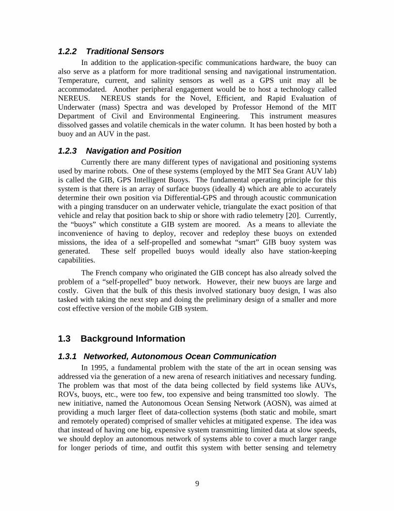
1.2.2 Traditional Sensors In addition to the application-specific communications hardware, the buoy can also serve as a platform for more traditional sensing and navigational instrumentation. Temperature, current, and salinity sensors as well as a GPS unit may all be accommodated. Another peripheral engagement would be to host a technology called NEREUS. NEREUS stands for the Novel, Efficient, and Rapid Evaluation of Underwater (mass) Spectra and was developed by Professor Hemond of the MIT Department of Civil and Environmental Engineering. This instrument measures dissolved gasses and volatile chemicals in the water column. It has been hosted by both a buoy and an AUV in the past.

1.2.3 Navigation and Position Currently there are many different types of navigational and positioning systems used by marine robots. One of these systems (employed by the MIT Sea Grant AUV lab) is called the GIB, GPS Intelligent Buoys. The fundamental operating principle for this system is that there is an array of surface buoys (ideally 4) which are able to accurately determine their own position via Differential-GPS and through acoustic communication with a pinging transducer on an underwater vehicle, triangulate the exact position of that vehicle and relay that position back to ship or shore with radio telemetry [20]. Currently, the “buoys” which constitute a GIB system are moored. As a means to alleviate the inconvenience of having to deploy, recover and redeploy these buoys on extended missions, the idea of a self-propelled and somewhat “smart” GIB buoy system was generated. These self propelled buoys would ideally also have station-keeping capabilities.

The French company who originated the GIB concept has also already solved the problem of a “self-propelled” buoy network. However, their new buoys are large and costly. Given that the bulk of this thesis involved stationary buoy design, I was also tasked with taking the next step and doing the preliminary design of a smaller and more cost effective version of the mobile GIB system.

1.3 Background Information

1.3.1 Networked, Autonomous Ocean Communication In 1995, a fundamental problem with the state of the art in ocean sensing was

addressed via the generation of a new arena of research initiatives and necessary funding. The problem was that most of the data being collected by field systems like AUVs, ROVs, buoys, etc., were too few, too expensive and being transmitted too slowly. The new initiative, named the Autonomous Ocean Sensing Network (AOSN), was aimed at providing a much larger fleet of data-collection systems (both static and mobile, smart and remotely operated) comprised of smaller vehicles at mitigated expense. The idea was that instead of having one big, expensive system transmitting limited data at slow speeds, we should deploy an autonomous network of systems able to cover a much larger range for longer periods of time, and outfit this system with better sensing and telemetry

9

instrumentation [18]. This goal requires “better” sensing instrumentation to be built, of course.

In line with this view of the future of autonomous communication is the research being described in this thesis. The communications buoy which the NEC has requested, could play a valuable role as a surface node in this type of air-sea data transfer. Additionally, a lot of the research which has been done developing and using underwater acoustic modems (UAM) on autonomous vehicles can be transposed to the buoy application. The software required to fully compliment and take advantage of the abilities of the underwater acoustic modem continues to emerge, and has yet to reach its full (and necessary) potential.

This network of inter-communicating vehicles and buoys has the potential to ameliorate the control and command process as well. Theoretically, a man sitting at a land-locked desk should be able to send a mission command by first communicating to a surface node, or satellite then surface node, and finally to not just one, but an entire fleet of underwater vehicles which are miles away. The “surface nodes” alluded to here directly encompass the types of technologies being explored in this thesis research.

1.3.2 History of Buoys Using buoys to transfer information obviously predates this research by many

years. Floating buoys have existed since before the 13th Century. These early buoys, as do many today, acted as signage for marine passages, just like ‘merge’ and ‘stop’ signs aid drivers today. In the Northeastern region of the United States, maritime commerce has been an absolutely vital part of the economy since pre-colonial times. The idea of a floating buoy as an aid to navigation was employed by the early settlers just as it is used by our modern day commercial fishermen. The first spar buoys appeared in Boston Harbor as early as 1780. [16]

In addition to the extensive network of navigational buoys which are used and maintained for the commercial fishing industry and its associated regulatory agencies, there is also a fleet of data collection buoys which serves an equally important role in aiding this industry. The National Data Buoy Center (NDBC), a branch of the National Oceanic and Atmospheric Administration (NOAA) under the U.S. Department of Commerce, owns and operates an extensive fleet of these types of buoys. As the NDBC so aptly states at their web-site, “moored buoys are the weather sentinels of the sea” [21]. Their systems provide the nation with information about barometric pressure, wind direction and speed, air and sea temperatures, and directional wave energy spectra. This information is used by scientists, meteorologists, fisherman, law makers, and others to issue forecasts, warnings, and models, as well as to aid ocean and meteorological research, emergency response programs, legal proceedings, and engineering designs. Ironically, the Metocean data provided by these buoys is the foundation for the design of subsequent data collection buoys, i.e. the one at the heart of this research.

There are many other secondary data buoy agencies around the nation which serve to augment the local assets of the NDBC. These second tier buoy networks are, in some cases, specially outfitted for their particular area of deployment. For example, TABS, the Texas Automated Buoy System, which is deployed in the oil-rich Gulf of

10

Mexico, is outfitted with scientific instrumentation which helps to monitor oil presence in the water. This system is thus able to aid in the prevention of and response to oil spills.

In the northeastern U.S. we have GoMOOS, the Gulf of Maine Ocean Observatory System. The first 10 buoys that GoMOOS ever deployed began taking hourly measurements of current, turbidity, dissolved oxygen, temperature, salinity and wave data in 2001. The GoMOOS project operates under the mission of bringing hourly oceanographic data to all those who need it. They specifically hope to aid commercial mariners, coastal/oceanic resource managers, scientists and public health officials. The data provided to these individuals via the GoMOOS network helps them monitor the ocean, and make decisions which directly effect the health and livelihood of our society. [17]

1.3.3 WAN In order to establish this buoy as an ‘access point’ for wireless Ethernet in an at-

sea LAN (local area network), it was necessary to choose a wireless protocol. This decision was made bearing in mind that this buoy might eventually be a single node in a whole network of buoys establishing a much larger-range LAN. This prototype buoy should rely on a standard Ethernet protocol; we chose 802.11b.

The 802.11 family of specifications was developed and accepted by the IEEE in 1997. It defines the over-the-air interface between a wireless server and a client, or two wireless clients. Within this family, there are four different specifications: 802.11, 802.11a, 802.11b, and 802.11g. They differ based on their prescribed frequency band, data transfer rate, and data transfer type – either frequency hopping spread spectrum (FHSS) or direct sequence spread spectrum (DSSS).

The 802.11b wireless Ethernet protocol became the standard for most homes and businesses in 2000. The WiFi alliance was created to maintain the 802.11b baseline of products and ensure interoperability. WiFi stands for “wireless fidelity” and bases its specifications on IEEE standards. Because WiFi is comparable to the “keeper” of 802.11b, the names are often used interchangeably. 802.11b is really an addition to the 802.11 protocol; they are backward compatible meaning that the ‘b’ version can send or receive data, but not both at the same time. 802.11b provides up to 11 Mbps data rates (with a fallback to 5.5, 2 and 1 Mbps). 802.11b nodes communicate in the very high (near microwave) frequency range (>2GHz), as opposed to traditional means of data transfer at sea which are near the VHF band. The actual performance of the network depends on the security measures in place. [23]

1.4 Project Management

Project management in naval architecture and ocean engineering is distinct in that unlike other engineering projects like cars and planes, the system is rarely mass-produced and rarely prototyped. Both of those characteristics are important from an economic perspective. Mass production is attractive because of the economies of scale that are introduced, but with offshore and other marine systems, each project has its own distinct

11

set of design constraints and requirements making almost every project a one-off production scenario [13]. Because the NEC Buoy project has an experimental aspect to its purpose, the potential for mass-production will only be evaluated after the long-term performance of the buoy is evaluated from a technological, endurance, and economic perspective. If, after operating for a substantial period of time, it is determined that the buoy does, in fact, effectively communicate information between submerged vehicles, ships, and shore and would, in fact, serve the commercial fishing community better if it were part of a networked array of similar buoys, then we may see the “mass-production” scenario become a reality. Prototyping is not common again partly because of scale. A jet engineer can prototype his design and explicitly verify his lift and drag estimates, for example, while a naval architect’s best hopes lie in the data taken from dragging a 1/200th scale model through a 200ft tow tank… provided the hydrodynamic understanding of the viscous, inertial and frictional forces acting on the hull was sufficient. A full-scale prototype of the NEC buoy is simply outside the financial means of the project. For this reason, it is more important that the dynamic model which is generated to establish heave and roll responses (etc.) is as accurate as possible.

1.4.1 Schedule and Budget The NEC Buoy design, fabrication and testing was on a tight timeline from the

onset of the project. The design phase began in December of 2003. Initially the testing dates were proposed for April of 2004. The original plan was to spend the entire month of January in the design process, then begin procurement and machining through February, and finally assemble and test for the first few weeks of March, allowing for a week of slack at the end if things were to fall behind. This plan turned out to be unrealistic with respect to the design phase. Due to difficulties with the heave analysis theory and application, design work continued through March, and then the solid modeling and shop-drawing generation continued through the first 2 weeks of April. Fabrication was delayed until the end of May and through June. Testing began in July of 2004. Given the brevity of the overall project life, however, it’s hard to believe that this does not compare favorably with the performance of many industry professionals in the field of ocean engineering and naval architecture.

The grant provided by the Northeast Consortium was for 24,000$. Part of that was meant to supplement engineering man hours at the MIT Sea Grant AUV Lab. The budget estimate for the buoy project, including hardware and machining only was approximately 18,000$. The as-tested version of the buoy cost closer to 11,000$ because it was not outfitted with the WHOI acoustic modem and because the batteries and solar panels cost less than 1/3 of what was estimated.

1.5 Buoy options There are two main types of buoys which are used in these types of applications: the discus buoy and the spar buoy. Each has distinctive characteristics that warrant its use in varying operational environments. No bias existed towards either buoy type with respect to the mission of this research. Both buoy types were researched and considered

12

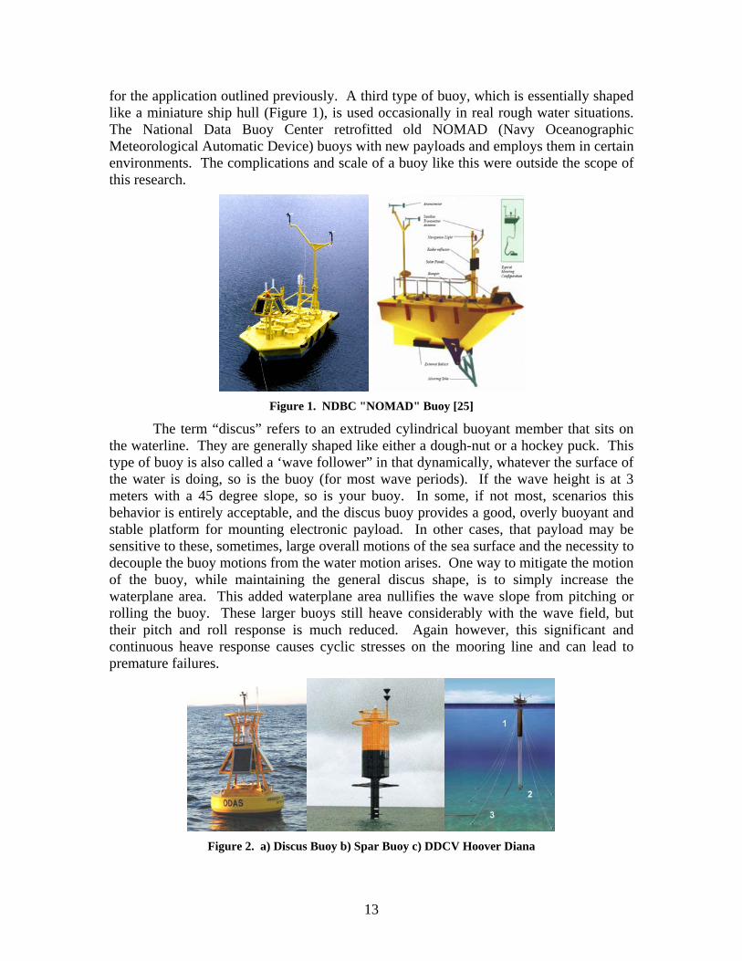
for the application outlined previously. A third type of buoy, which is essentially shaped like a miniature ship hull (Figure 1), is used occasionally in real rough water situations. The National Data Buoy Center retrofitted old NOMAD (Navy Oceanographic Meteorological Automatic Device) buoys with new payloads and employs them in certain environments. The complications and scale of a buoy like this were outside the scope of this research.

Figure 1. NDBC "NOMAD" Buoy [25]

The term “discus” refers to an extruded cylindrical buoyant member that sits on the waterline. They are generally shaped like either a dough-nut or a hockey puck. This type of buoy is also called a ‘wave follower” in that dynamically, whatever the surface of the water is doing, so is the buoy (for most wave periods). If the wave height is at 3 meters with a 45 degree slope, so is your buoy. In some, if not most, scenarios this behavior is entirely acceptable, and the discus buoy provides a good, overly buoyant and stable platform for mounting electronic payload. In other cases, that payload may be sensitive to these, sometimes, large overall motions of the sea surface and the necessity to decouple the buoy motions from the water motion arises. One way to mitigate the motion of the buoy, while maintaining the general discus shape, is to simply increase the waterplane area. This added waterplane area nullifies the wave slope from pitching or rolling the buoy. These larger buoys still heave considerably with the wave field, but their pitch and roll response is much reduced. Again however, this significant and continuous heave response causes cyclic stresses on the mooring line and can lead to premature failures.

Figure 2. a) Discus Buoy b) Spar Buoy c) DDCV Hoover Diana

13

The spar buoy addresses this problem of surface decoupling and reduced motion. In general, the word “spar” refers to any long, structural member used to support either sails, or rigging, or even the aluminum plates on an airplane wing. Associated with the concept of a buoy, the word spar refers to the relative geometry of a marine structure which is long and slender, oriented roughly perpendicular to the ocean surface, and whose buoyancy is distributed along its draft as opposed to just the waterline. Spar buoys have been used extensively in ocean science and exploration. A type of spar has been adapted (and greatly scaled up) by the offshore industry to act as an oil production platform. The industry calls these Deep Draft Caisson Vessels (DDCV, see Figure 2.c) and has installed them in some of the deepest applications.

1.5.1 Others out there? Most engineering design projects start with a study of existing systems. In naval

architecture this is called a “similar ships study”. This process involves researching existing vessels which serve the (nearly) same purpose in the (nearly) same environment as your intended project. The characteristics of these pre-existing vessels provide a baseline design for the current project which can be further tweaked to an optimal point. This same idea was employed for this buoy project. First, because it provided the obvious benefit of finding out what the typical geometric and hydrostatic scales and ratios are for this type of buoy, and second, because if there were to be a commercially available buoy which would serve as a sufficient infrastructure on which to build up the system we are eventually hoping to have, then that may be a financially viable (and favorable) option. Budget considerations immediately presented the option of acquiring an off-the-shelf communications buoy and fitting it to our design requirements once in house. The advantages of this would be, of course, major time savings, cost savings, and the benefit of a proven buoy concept. The disadvantages of this idea are the inefficiency of a design not intended for our exact use and our exact hardware size/orientation. The idea that purchasing a ready-made buoy would save money in the long run was later disproved.

Looking, at first, for buoys with the purpose of aiding the work of commercial fisherman, the ComBeacon was discovered. This product is made by an Australian company called Commercial Catamarans in direct response to the needs of local tuna fisherman. The ComBeacon is a spar type buoy with a 30-day endurance between battery recharges. It provides 12-channel GPS communications in a 100 mile radius. Because this buoy was designed by a fisherman for a very narrow purpose, it is not generic enough to serve our purpose and is too small to support the full payload that we must impose.

The closest system, with respect to displacement and mission that was identified belonged to Hydroid Inc. of Falmouth, MA. This WHOI spin-off company generated the ‘Paradigm’ (Portable Acoustic/RADio Geo-referenced Monitor). This buoy is intended to act in tandem with another (or many other) identical buoys to acoustically track a vehicle anywhere within a 2 kilometer radius. The buoy can then transmit this info up to 20 miles via radio telemetry. This system is very expensive, ~18K, and still not big enough to float the instrumentation which we intend to use. The cost of the basic system would nearly sap the budget, and would still need to be retrofitted with multiple,

14

additional, and expensive instrumentation. It is also not clear if this buoy would be able to withstand the design survival sea condition of Sea State 4.

OCEANOR and Ocean Science both produce data buoys which are not of the spar type and provide a much larger floating platform than required for the NEC system. OCEANOR’s SeaWatch Buoy is meant for wave and wind measurements with limited telemetry instrumentation. The Ocean Science SeaBuoy provides 920 kg of buoyancy, which is well outside the required displacement. Sound Ocean Systems, Inc. of Washington State also offers an oceanographic data buoy but also saturates the needs of the current system with its 24 month power endurance and 730 kg displacement. All of these systems were economically unrealistic for our intended use.

In the search for similar buoys, multiple companies and private research institutions surfaced which have made and, in some cases, market a spar-type, communications buoy. Observing the relative dimensions and geometries of these existing buoys was a good exercise for the designer, however the prevailing observation was that these existing systems were either entirely too big and saturated the requirements (and budget) for the NEC buoy, or the exact opposite. There were many very small (~40kg displacement) spar buoys out there that could be handled with one hand. If power endurance wasn’t an issue and we didn’t need to mount a 2m antenna mast to the top, these buoys might have been sufficient. Finally, it was determined that spar buoys made for similar purposes as the NEC system do exist, but those with reasonable costs and potential as an infrastructure for our in-house electronics and power systems do not. Unfortunately the disadvantages explained above combined with the lack of availability of appropriately sized spar options, forced the design and construction to be completed in house. An aside: if it were to become necessary to chose one of the existing systems as opposed to manufacturing one in-house, the Hydroid Paradigm would probably be the most appropriate given its size, mission, and the proximity of the manufacturer to the test site.

1.5.2 Spar characteristics and justification One of the main things that was taken into account when determining which buoy

type should be used for this application was the motion sensitivity of the communications systems. In order to maintain constant contact with an onshore antenna in sea states up to SS4 conditions, the heave and roll response of the buoy must be minimized. Additionally, the environmental design criteria also forced certain length scales. For example, if a spar were to be used, the freeboard and length of the reduced-diameter section would be somewhat dictated by the maximum wave amplitude.

Ultimately, the spar buoy was favored for this application because of its superb heave and roll characteristics when properly designed. This decision is made with the understanding that there is limited experience with spars of the approximate displacement that we intend. Spar buoys which have been designed for scientific and communications purposes, and also need to withstand the same sea states as is presently required, are generally much larger than we intend. The DEOS spar, a design project sponsored by the NSF which included WHOI engineers, is on the order of 133 feet long [8]. Dynamic performance is necessary for the success of the communications part of this project, but it is yet to be seen how a spar on this smaller (~10ft) scale will perform. Thus, although it

15

is undoubtedly expected that a spar buoy will heave and roll much less than its discus counterpart, using this type of design is somewhat experimental and adds to the value of the results of this work.

16

2. Environmental Design Criteria

A complete physical and statistical description of the proposed operating environment is a vital component of the design process. The information contained within the sea spectra does more to dictate design requirements than any client ever could. Natural frequencies, relative geometries and scale, and other static and dynamic response characteristics are largely defined by the significant wave height and period of the seas, the direction/interaction of the sea and swell condition, and other metocean (shorthand for meteorological and oceanographic) data.

The design criterion for the buoy requires operability in Sea State 3 and survivability in Sea State 4. In order to more adequately outline what this means for the buoy design, field data was taken from buoys in the proposed operating environment. This data was then analyzed to give the reader a better understanding of the seas which will be experienced by the buoy, and also to ensure that it is compatible with the common sea spectrum approximations. This comparison of field data with a derived spectrum is important in the respect that most offshore projects cannot afford to be overdesigned. If it were adequate to make every system much larger than necessary with ample factor of safety, then it would never be necessary to have a complete understanding of the environment.

2.1 North Atlantic

The NEC buoy was designed to operate approximately 1 mile off of the eastern tip of Cape Ann. MIT Sea Grant has a working relationship with the local fishermen and maintains an aquaculture site in that area. Because of these associations, there should be no trouble establishing a shore node and setting up a directional antenna.

2.1.1 Wave Data There are two nationally recognized data buoys located in the relative vicinity of

the proposed deployment position, first is a National Oceanic and Atmospheric Administration (NOAA) buoy and the other is part of the Gulf of Maine Ocean Observing System (GoMOOS) (Table 1). Via the NOAA and GoMOOS websites, wave data was downloaded for October through January of 2003/04 (~100 days). Only these four months were analyzed because the buoys take approximately 15-24 readings per day – a lot to deal with, and the two different buoy operators publish the data in different formats which made it impossible to write a scheme which would automate the analysis procedure. These four months are considered a conservative estimate of the sea state distribution.

The wave data analysis procedure involved finding the significant wave height along with the significant wave period for each day, and then assigning a Sea State value for that particular day based on the SS definition table published at www.oceandata.com .

17

ID Number Identifier Operator Latitude Longitude 44013 Boston East NOAA 42˚21’14” N 70˚41’29” W 44029 Mass Bay- Stellwagen Bank GoMOOS 42˚31’40” N 70˚33’59” W

Table 1. Data Buoy Definitions

Figure 3. Data Buoy Map [17]

For this preliminary set of data, there are a few immediate observations to be

made. The GoMOOS buoy 44029, as it is located farther off shore, sees a wider range of sea conditions and is characterized most often (28.15% of the time Oct-Jan) by Sea State 3. SS3 is characterized by wave heights between 3.5 and 4ft and average wave periods of approximately 4 seconds. The NOAA buoy 44013, located closer to shore within the Boston Harbor, observes Sea State 2.5 (2.5-3ft significant wave heights and 3.5sec wave periods) 35.87% of the time during October through January. Figures 4, 5 and 6 illustrate the sea state and wave height probability of occurrence histograms from the buoy data. [17, 21]

Another observation is that at the Mass Bay location, there is a 47% chance that on any given day you will see a sea state greater than 3, and at the East Boston location, on any given day there is a 25% chance of Sea State 3.5 or greater. These statistics are only valid in the wintry, and often stormy, months of October through January. This was considered a conservative sample.

0

5

10

15

20

25

1 3 5 7 9 11 13 15 17 19 21 23 25 27 29

wave height [m]

prob

of o

ccur

renc

e %

Figure 4. Wave Height Histogram for 44029

18

0

5

10

15

20

25

30

1 1.5 2 2.5 3 3.5 4 5 6 7

Sea State Identifier

Prob

abili

ty o

f Occ

uren

ce (O

ct-J

an)

Mass Bay 44029

Figure 5. Sea State Histogram for GoMOOS Buoy 44029

0

5

10

15

20

25

30

35

40

1 2 2.5 3 3.5 4 5 6 7

Sea State Identifier

Prob

abili

ty o

f Occ

urre

nce Boston Harbor 44013

Figure 6. Sea State Histogram for NOAA Buoy 44013

Table 2 is the reference used to characterize the wave data into relative sea states

as seen in Figures 5 and 6. Table 2 data assumes fully developed seas.

Sea State

Significant Wave (Ft)

Significant Range of

Periods (Sec) 0 <.5 <.5 - 1 1 0.5-1 1 - 4 2 1.5-2 1.5 - 5

2.5 2.5-3 1.5 - 6 3 3.5-4 2 - 7

3.5 4.5-6 2.5 – 7.5 4 6-7.5 2.5 - 9.5 5 8-12 3 - 12 6 14-20 4 – 15.5 7 25-40 5.5 - 22

Table 2. Sea State Definition [26]

19

2.1.2 Current and Tide Data In addition to being important with respect to the buoy dynamics, information

about the current profile, tides, and air speed is also necessary for the mooring design and analysis. The current profile at a given location helps to dictate what the safe weight of the anchor will be in order to maintain the mooring position. Tide data could only be found on the NOAA site for the Boston Harbor as a whole. The average tidal fluctuation is approximately 3.5ft [21]. Using mooring line simulators and this data, you can estimate the static offset of the buoy away from the anchor point. This information leads to a better understanding of the buoy “watch circle”.

Current patterns in the Gulf of Maine are a direct result of the shape of the coastline. Flow speed and direction, in general, is dependant on the wind, the rotation of the earth, landmasses and water density.

Figure 7. Mass Bay Buoy 44029 Current Measurements [17]

NOAA Buoy 44013 does not have acoustic Doppler current profiling capabilities, while the Mass Bay GoMOOS buoy does. Most of the GoMOOS buoys are outfitted with instrumentation to measure surface current speed and direction at 2 meters and then throughout the water column at 4m intervals. Figure 7 is current speed data taken from the GoMOOS Mass Bay location between December ’03 and January ‘04. The hourly data was averaged over the time period at each depth in order to produce Figure 8 below, which represents the current “profile” at this location.

20

-70

-60

-50

-40

-30

-20

-10

00 0.05 0.1 0.15 0.2

Current Speed [m/s]

Dep

th [m

]

Figure 8. Mass Bay Buoy 44029 Current Profile

2.2 Alternative Operating Environments

Although this buoy was designed specifically for sea state 3 and 4 conditions in the waters off of Cape Ann, the possibility remains that it might eventually be deployed in a more benign operating environment. For a research group working in the Cambridge, MA area, this often implies the Mystic Lake or the Charles River. The MIT AUV Lab has used the Mystic as a shallow-water, closed testing and operating environment in the past. Other than the fact that it may freeze in the winter and is host to incessant recreational sailing at all times of the year, the most menacing sea state, or better said “lake state”, to be found on the Mystic is a developed chop with random, high frequency, relatively low amplitude wave components, which are of course effected by the shape and location of the shore. The Charles River is more affected by the Harbor tides and the upstream activity. The river has locks both up and down stream and the water level can change significantly in a day.

The NEC Buoy was designed to operate in a harsh environment and for that reason would appear over-designed in either the Mystic Lake or the Charles River. However, its ability to perform the functions required by the hosted electronics should not be compromised by these alternative conditions. The major issue to be addressed between operating the buoy in the open ocean and a closed, fresh-water environment is the varying salinity. The density of the Mystic Lake (~1000kg/m3) is somewhat less than that of the sea (1025 kg/m3) because it is fresh water, as is the Charles River with its brackish water. The varying water density affects the amount of buoyancy required to float the payload in any given configuration

21

2.3 Final Sea State Model

Although true field data was available for the deployment site, the Sea State was modeled with a Bretschneider Spectrum using as input the significant wave height and period of the design sea states. For this analysis, fully developed seas were assumed although the Bretschneider is capable of handling developing seas as well. The available data behaved like this theoretical spectra and therefore, for simplicity’s sake, was set aside in favor of using Bretschneider.

The only immediately obvious shortcoming of the Bretschneider spectrum is that it does not take wave slope into account [14]. The Bretschneider also does not address the directionality of a sea condition; however, this is a conservative oversight. The Bretschneider Spectrum is shown both in equation and graph form below. Sea State 3 conditions were modeled with Hsig=1.22m , and Tsig=4.5sec. Sea State 4 was modeled with 2.3m significant wave height and 5.5 second wave period.

4)(25.12

5

4

425.1)( ωω

ωωω neHS sig

n −+ =

Figure 9. Bretschneider Model

2.4 Wave Statistics

Because the sea is generally assumed to be a superposition of many simple, linear, harmonic wave components, engineers often use probability and statistics theory in their analyses. Often however, design constraints originate in the condition of the sea during a storm or some other short-term event. For example, although an offshore platform might be (and usually is) designed for a wave event that happens only once in 100 years, it might never see that wave in its 20 year life span. Or conversely, if it does, the sea

22

conditions associated with that 100-year wave event only last for a couple of hours. Therefore, we not only consider the statistics of the environmental conditions but also their probabilities of occurrence during short spans of time and over the longer term life-span of the system. This discussion is relevant with respect to the NEC Buoy because the design criteria mention Sea State 3 and 4 conditions, which are both short term definitions of a fully developed state.

2.4.1 Spectral Analysis The use of the statistical sea-state analysis method requires an understanding of

spectral theory in general. The theory involved with the spectral analysis of a random process imposes certain assumptions about the sea state you are attempting to model. First, in order to prove the process is homogeneous, one must confine the implications of their analysis to within a certain area of the sea, namely the area where the storm or sea event is taking place. This “area” can range from a couple square nautical miles up to, say, 500. Additionally, we can only maintain the implications of stationary process analysis by assuming the spectrum is valid only over a limited period of time, a couple of hours. Once these assumptions are understood, we can move on to employing the full range of tools that spectral analysis offers. [4, 6]

Theoretically, all spectra can be “double sided” meaning there is a positive frequency component as well as a negative frequency component. For environmental modeling purposes, only the positive frequency component is taken into account. The common spectrum is often described by making use of its “moments”. Some basic quantitative characteristics of a spectrum are outlined in equation form below.

A very common statistic is the “Zeroth Moment”:

∫∞

+=0

0 )( ωω dSM … or the area under the spectrum

oddnevenndSM

n

n __

0

)(0

⎪⎩

⎪⎨⎧

= ∫∞

+ ωωω

For narrow banded spectrum

03/1 4 MH ==ς and ςω /4.0 gm =

0MH RMS =

The probability density of the random process that defines the sea surface is generally assumed to be Gaussian. Gaussian distributions assume that the wave record is symmetric about the still water level, which means it has zero mean. (This assumption holds for waves of normal to moderate amplitudes but breaks down with very large amplitudes.) [6] The density of the sea elevation is given below.

23

2

2

2

21)( ησ

η

ηπση

−

= ep

where the variance, 0M=ησ

Keeping in mind the fundamental difference between the wave elevation and the wave amplitude, we can further describe the probability density function of the wave amplitude.

0

2

2

0

)( Ma

eMaap

−

=

From the probability density function for the wave amplitude we can look at the statistics of the wave height (twice the amplitude). Again, assuming a normal distribution, the equations below describe some of the common information taken from this relationship.

The most frequent wave height, hm:

RMSm HH 707.0=

The average of the 1/nth highest wave heights:

03/1 005.4 MH = 010/1 091.5 MH = 0100/1 672.6 MH =

The most probable maximum wave height in 100 and 1000 waves are:

3/1100 534.1 HH MAX = and 3/11000 86.1 HH MAX =

2.4.2 Short term In general, there are two methods for choosing design wave environments. The

first involves simply choosing a single design wave represented by a wave height and natural period, and the second involves choosing an appropriate wave spectrum from those which have been empirically generated over the years. The chosen spectrum should appropriately represent the distribution of waves in the area of deployment [5]. There exists a range of established spectral formulations which require only a significant wave height, which is the average of the 1/3 highest wave heights, and a period. These spectra describe only a short term sea condition. The best possible option in this respect is obviously by taking field data and actually generating the true wave spectrum for the site. Because of the fortunately close proximity of the NOAA and GoMOOS data buoys to our buoy site, we had this option. It was observed, however, that the Bretschneider representation was not only a sufficient match to the observed data but also a slightly conservative design spectrum.

For our application, the buoy was designed under the Bretschneider representation of a SS3 operational condition and SS4 survival condition. The design could then be further engineered to withstand these conditions and the wave heights that are associated

24

with 99% (or some other similarly high probability) chance of non exceedance. Again however, these short-term statistical analyses are only valid for a period of a couple days, while the storm, or sea condition, retains its basic characteristics. Table 3 outlines the short term statistics for the SS3 and SS4 conditions used to design the NEC Buoy.

Sea State 3 Sea State 4

ζ=H1/3 1.22 m 2.3 m

Tsig 4.5 sec 5.5 sec

M0 0.0929 0.3305

M2 0.3456 0.8331

M4 2.7328 4.9171

HRMS, ση 0.3048 m 0.5749 m

Hm 0.2155 m 0.4065 m

H1/10 1.552 m 2.927 m

H1/100 2.034 m 3.836 m

HMAX100 1.87 m 3.53 m

HMAX1000 2.27 m 4.28 m

Table 3. Wave Statistics

25

3. NEC Buoy Design and Analysis

3.1 Design Overview

3.1.1 Scale and Dimension The original conception or expectation of the size of this buoy was considerably

smaller than the final design. There were three very important factors which necessitated the final dimensions of the NEC buoy. First, the Metocean criteria introduce minimum draft limitations as well as a minimum mast height. The reason why a good spar buoy design has minimal heave response is because the wave crests are able to climb up and down a skinny, surface-piercing neck section without contacting either the super structure or the buoyant tank(s) below. The spar buoy should be designed with the main buoyant portion located well below the DWL, and with enough freeboard that the topside platform isn’t contacted by most waves. The actual minimum values for these distances should be calculated using a factor of safety times the average maximum wave amplitude.

The second reason for the scale of the buoy is also related to the subsequent dynamic response and its relationship with the sea condition. Because the typical spar design does not have a significant moment of inertia at the water plane, roll stability must be made up for with sufficient spacing between the vertical center of buoyancy (VCB) and the vertical center of gravity (VCG). The ocean vessels which are known to be overly stable in roll are often those with beamier hulls and ‘fatter’ or fuller sectional areas. The reason for this is because, given a unit roll angle, the vessel is picking up a significant amount of newly submerged buoyant volume and has a larger transverse metacentric height. The spar does not exhibit this quality. In fact, the entire idea behind the spar design is to minimize the surface piercing area with a single strut like member. These roll characteristics, again, encourage a deeper draft, or larger draft/diameter ratio, in spar design.

The third explanation for the general scale of this spar design stems from the space and logistics requirements of the electronic payload and power system. One of the main reasons why the smaller, 40kg displacement, spar buoys which were found to be commercially available emerged as unfeasible options for this project, is because they could not physically accommodate the battery system and the computer stack. As opposed to the first two scale constraints which encouraged draft, this limitation is more important in reference to the spar diameter.

3.1.2 Design Process The NEC Spar buoy was designed under the following guidelines:

- Survival condition: Sea State 4 : H1/3=2.3m and Tavg=5.5sec - Operational condition of SS3 : H1/3=1.22m and Tavg=4.5sec - Significant Heave Response Magnitude less than 50cm - Significant Roll Response magnitude less than 30° - Significant Roll Rate magnitude less than 5.5°/sec

26

- Servicing at ~2 month intervals - Serviceable by 2 guys on a smaller vessel (ideally without an A-Frame) - 150kg weight limit - Up to 300m water depth

The sea state design criteria dictate that using the conditions characteristic of a sea

state 3 and 4 storm event, the communications systems will work and the buoy will not break. The communications electronics are assumed to function best at or below the specific heave and pitch magnitudes and rates outlined above according to the Harris Corporation of Ref [8]. Therefore, this design constraint was enforced by using the spectra representative of each sea state and ensuring the buoy did not exhibit motions outside of those velocities/accelerations.

From these requirements, there were actually multiple buoys designed. Each of them addressed a different major concern of the MIT Sea Grant AUV Lab engineers who would eventually be in charge of deploying and maintaining the system. The first design, which I refer to as the foam buoy, was extremely modular, light weight when in pieces but heavier when together, and allowed for the modularized payload and power systems to be accessed and removed without removing the entire buoy.

3.1.2.1 Phase I: The ‘Foam Buoy’ Design Throughout the design process, one particular variation had risen to the forefront.

The work done on this design, we’ll call it the foam buoy (Figure 10), had encompassed all planned design time and had passed previous reviews throughout its development. However, rising concerns regarding the weight of any system, regardless of shape, had emerged and it was at this point that a weight limitation was imposed. The system was now not to exceed 150 kg. The most current design then, the foam buoy, surpassed that by nearly 30 kg.

The foam buoy was designed for a dynamic payload, meaning the structure and payload “bay” was made to be modular and easily adaptable. For example, instead of making one rigid payload frame, there are multiple inner frames pre-engineered with numerous holes and points of attachment. There is also space for almost 150% more buoyant reserve than used for the current displacement requirement. Instead of having the lower buoyant section be locked into a fixed volume, it was designed such that the larger diameter portion of foam could be segmented and used only in part. Or, for minimal buoyancy, the baseline, smaller diameter foam pieces are used the full draft of the buoy. Allowing for this light configuration could potentially prove valuable if the researchers need to remove the communications electronics and/or power systems and leave the buoy on site in its lightest state for an extended period of time.

27

Figure 10. Foam Buoy Design

Obviously the field life of the buoy without battery recharge is a more compelling constraint than a weight limitation. Especially considering the fact that even at only 100 kg, the geometry of a 2m spar buoy is difficult for 2 guys to manage on a smaller fishing vessel. The concerns about weight were valid none-the-less and an entirely new design was initiated. This new one, which was built, does not use foam as a means to float many smaller sealed containers. The new design draws its buoyant volume from the structural members instead of in addition to them. Because of this however, the foam buoy design is much more conducive to significant increases in payload size.

3.1.2.2 Phase II: The Hollow Aluminum Buoy Design The second NEC Buoy design iteration addressed the fundamental concern which

was identified through the first design review, namely, that the weight of the foam and outer protective structure was superfluous with respect to the weight of the payload. Ratios of structural weight to total displacement were discussed for stiffened marine bodies (approximately 0.4 or less), and the general consensus was that with this first design we were in a sense “paying too much” in overall weight to float a limited payload weight. Between 50-60% of the overall weight was found in structural elements. One of the defending arguments against these concerns and in favor of the first design was that the scale of this mid-range spar buoy was determined more by metocean criteria than the payload requirements. The wave height and period forced the minimum draft and hydrostatic characteristics, and since overall weight is strongly correlated with physical size there wasn’t much one could do to decrease this weight. Simply put, designing a spar for the coastal Cape Ann area requires at least this size and weight. Switching design philosophies and settling for a wave-following buoy would help to decrease the overall weight, but would not exhibit sufficiently low heave and roll responses to sustain the communications mission of the buoy; without which, the entire system need not exist. Nonetheless, a new design which eliminated the foam and outer structure was generated. Figure 11 depicts the three designs considered in this second iteration.

28

Welded Aluminum, Cylindrical

Figure 11. Phase II Design Considerations

Incorporating the concerns which surfaced from the first phase of the design process with the overall physical and dynamic requirements for a buoy of this type, the final design was established.

The primary difficulty which was encountered in this second phase of design, which focused on an aluminum shell buoy structure, was maintaining a high enough vertical center of buoyancy. The VCB, as it is called, is defined as the centroid of the submerged volume. It is important that the weight stay centered as low as possible, which often implies that the payload itself is kept low unless a ballast tank is allowable. Payload of the type found on the NEC Buoy must, of course, be housed in a water tight container, and based on the geometry of this payload, especially the power system, this container is generally large. Both fortunately and unfortunately, large, water-tight containers are wonderful sources of buoyancy, and while needed low to house the payload, they bring the center of the submerged volume lower as well which is not a desired effect. This challenge of maintaining a high enough center of buoyancy while keeping the weight low is a characteristic of all naval architectural systems, but is much more intricate for a spar configuration, and is also why most spars are so very long with buoyant tanks located well above their “keel” while still well below the waterline.

The final NEC Buoy design (Figure 12, Table 4) takes into account all of the design requirements and general logistics issues. It is not a 100% optimized design, but will certainly serve its purpose and exhibits good seakeeping characteristics for its mission as a communications platform.

House Batteries

Submerged Battery Can(s)

Box

29

l1

l3

l2 d2

d3

d4

d1

LOA 3.4m

Mast Height 1.5m

Draft 2.6m

d1 0.15 m

l1 0.75 m

d2 0.25 m

l2 1.12 m

d3 0.15 m

l3 0.66 m

d4 .61 m

Batt Can Diameter

0.30 m

Batt Can

Length

0.43 m

Table 4. Buoy Dimensions Figure 12. Final NEC Buoy Design

3.1.3 Weight Estimate Weight and balance work is often the first assignment given to a naval architect

fresh out of school. This aspect of the design process carries with it the stigma of being simple, tedious, and somewhat annoying while at the same time extremely important to the success of the project. An accurate weight estimate is absolutely vital, especially in systems which are designed to have little excess buoyancy, because even the smallest mistake can cause the system to sink. Having to ballast a vessel because of a minor error in draft estimation is nothing compared to the technical difficulty (often impossibility) and professional shame associated with retrieving a sunken structure off the ocean floor.

With the design of systems, like this buoy, which have somewhat dynamic mission requirements and payload, it is difficult to pinpoint an exact list of cargo. The buoy should be able to float the same for mooring situations in water depths up to 300m and with varying cargo loads. However, the most prevalent water depth in the coastal Cape Ann zone is only around 100m. For most mooring line products there is a significant weight difference between 100m of line and 300m. Shallow water mooring conditions and light load configurations will require ballast weight be incorporated on the buoy. Table 5 shows a rough weight estimate, with loads given under major system headings.

30

Group Weight Units

Hull Structure 66.4 kg Mooring System 15 kg Communications 6.8 kg

PC Housing 4.85 kg GPS and other sensors 1 kg

Battery system 37.9 kg Acoustic Comms 5.2 kg

Totals 137.15 kg

Table 5. NEC Buoy Weight Estimate

3.1.4 Basic Statics The hydrostatic characteristics of a spar buoy are interesting from a conventional

naval architectural perspective because they challenge the common understanding of what makes a vessel “stable”. The intuition bred into the budding naval architect is that beamy is better. The spar buoy, when engineered correctly, exploits the narrow opportunity for stability in a deep-draft, slender-body design. The typical assumption that the wavelength of the seas is much greater than the predominant length scale of the body is taken to the extreme with spar design.

The evaluation of the array of designs which were considered for the NEC Buoy emphasized the idea that there is a narrow range of scales and length ratios where the spar is a viable and stable floating platform. Achieving sufficient draft to ensure a positive righting moment was often difficult. Table 6 outlines the hydrostatic characteristics of the NEC Spar design.

[sec]2v

heaveHeave m

CT ⋅= π [sec]2v

RollRoll I

CT ⋅= π

Cheave and CRoll are the spring constants or coefficients of the restoring force in each degree of freedom. They are found via the following relationships [1, 3]:

wpHeave gAC ρ= gmgmgVCRoll ⋅∆=⋅= ρ

VCG (w/ mooring) 1.02 m VCB 1.16 m

VCG (w/out mooring) 0.87 m Awaterplane 0.02 m2

∆ 137 kg ωHeave 0.75 rad/sec

Volume 0.134 m3 THeave 8.4 sec

BG (w/mooring) 0.29 m ωRoll 1.31 rad/sec

BG (w/out mooring) 0.13 m TRoll 4.8 sec

Table 6. NEC Buoy Hydrostatic Characteristics

31

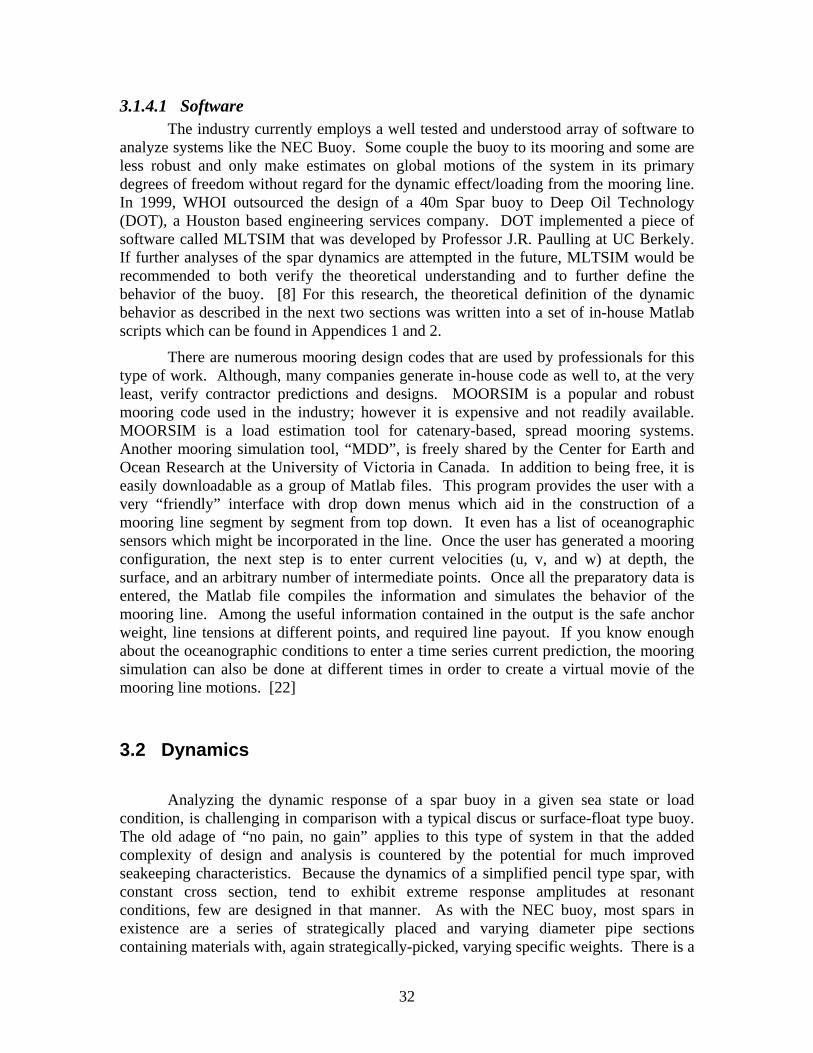
3.1.4.1 Software The industry currently employs a well tested and understood array of software to

analyze systems like the NEC Buoy. Some couple the buoy to its mooring and some are less robust and only make estimates on global motions of the system in its primary degrees of freedom without regard for the dynamic effect/loading from the mooring line. In 1999, WHOI outsourced the design of a 40m Spar buoy to Deep Oil Technology (DOT), a Houston based engineering services company. DOT implemented a piece of software called MLTSIM that was developed by Professor J.R. Paulling at UC Berkely. If further analyses of the spar dynamics are attempted in the future, MLTSIM would be recommended to both verify the theoretical understanding and to further define the behavior of the buoy. [8] For this research, the theoretical definition of the dynamic behavior as described in the next two sections was written into a set of in-house Matlab scripts which can be found in Appendices 1 and 2.

There are numerous mooring design codes that are used by professionals for this type of work. Although, many companies generate in-house code as well to, at the very least, verify contractor predictions and designs. MOORSIM is a popular and robust mooring code used in the industry; however it is expensive and not readily available. MOORSIM is a load estimation tool for catenary-based, spread mooring systems. Another mooring simulation tool, “MDD”, is freely shared by the Center for Earth and Ocean Research at the University of Victoria in Canada. In addition to being free, it is easily downloadable as a group of Matlab files. This program provides the user with a very “friendly” interface with drop down menus which aid in the construction of a mooring line segment by segment from top down. It even has a list of oceanographic sensors which might be incorporated in the line. Once the user has generated a mooring configuration, the next step is to enter current velocities (u, v, and w) at depth, the surface, and an arbitrary number of intermediate points. Once all the preparatory data is entered, the Matlab file compiles the information and simulates the behavior of the mooring line. Among the useful information contained in the output is the safe anchor weight, line tensions at different points, and required line payout. If you know enough about the oceanographic conditions to enter a time series current prediction, the mooring simulation can also be done at different times in order to create a virtual movie of the mooring line motions. [22]

3.2 Dynamics

Analyzing the dynamic response of a spar buoy in a given sea state or load condition, is challenging in comparison with a typical discus or surface-float type buoy. The old adage of “no pain, no gain” applies to this type of system in that the added complexity of design and analysis is countered by the potential for much improved seakeeping characteristics. Because the dynamics of a simplified pencil type spar, with constant cross section, tend to exhibit extreme response amplitudes at resonant conditions, few are designed in that manner. As with the NEC buoy, most spars in existence are a series of strategically placed and varying diameter pipe sections containing materials with, again strategically-picked, varying specific weights. There is a

32

balancing act which takes place while the designer is attempting to get sufficient distance between the vertical center of gravity (“weight low”) and vertical center of buoyancy, and also trying to minimize size and cost. These conflicting design objectives often push the overall draft of the spar to growing lengths.

A good understanding of the response spectra of the NEC buoy in a given sea state is necessary for maintaining uninterrupted communications contact as well as safe-guarding the buoy structure and mooring from failure. In order to describe the motion of any physical system, there must be a complete and accurate outline of the static and dynamic loading present. This is the first step in the hydrodynamic analysis of a naval architectural system.

3.2.1 Hydrodynamic Loading Wave forces on floating bodies are generally estimated using Morsion’s Equation,

Froude-Krylof Theory, or Diffraction Theory. Morison assumes inertial and drag force components are linearly superimposed. This is most applicable for small structures (where L<<λ) and used mostly in drag dominated scenarios. If the structure is small but inertial forces are significant, Froude-Krylof force estimation is employed. Froude-Krylof is based on computing the pressure force on the body surface from wave elevation effects and was employed extensively for the NEC Buoy heave analysis. Finally, for very large structures (where L~λ), the wave field is effected by the presence of the structure therefore diffraction theory must be used.

Integral to each of those force determination methods is the knowledge of certain hydrodynamic coefficients. Most of these coefficients are determined experimentally. We are most interested in the added mass, lift, drag and damping coefficients. Fortunate for the analysis of the spar buoy, a good number of experiments have been conducted on a vertical cylinder.

A vertical, cylindrical buoy in a current experiences friction and pressure forces along its length. When we assume that the flow is roughly laminar, shear stresses dominate. These sheer stresses are directly related to the drag felt by the buoy. The drag of a buoy which is roughly symmetric about its central axis is in the direction of the flow and is computed using the following equation. A is the projected area and V the velocity of the current.

2

21 AVCD D ρ⋅=

There is a second component to the drag or horizontal resistance force which is present for buoys of certain sizes, that is the wave making resistance. If our buoy were to be of such size that it diffracted wave crests and altered the wave field, this second component would need to be addressed using Diffraction Theory. [6, 5]

3.2.2 Heave Analysis The heave response of a spar buoy is important because ill positioned (with

respect to the sea spectra) natural frequencies can yield extreme motions. Although this degree of freedom is less important than pitch/roll when considering the acoustic and radio telemetry, its minimization is vital for structural and mooring purposes. In the

33

offshore industry, heave is of paramount importance because it directly effects the tensions in the mooring lines, but more importantly, the drilling and/or production risers can be fatally loaded also. Henri Berteaux [1, 2] offers a few warnings with respect to the heave response implications of certain design parameters. He does support the use of damping plates for further decreasing the heave response, however warns that placing them too close to the surface can actually amplify heave motion. This information is pertinent to the NEC buoy analysis because the plates which sandwich the battery can in the final design are intended to act as heave dampers. Berteaux also says, rather ideally, that “good spar buoys do not heave!” thereby saying that the upper pipe or “neck” section of the buoy should be long enough such that the incoming wave field can slosh around without ever revealing the presence of the buoyant tank sections below or the superstructure above.

3.2.2.1 Theory The method for determining the heave, or any other degree of freedom, response

of a floating system always starts with using Newton’s fundamental law: ΣF=ma. Regardless of how complex the system may appear, or how menacing its environment may be, this relation must always be true and, in its entirety, explains any possible motion, or combination there-of, that could possibly be witnessed. In heave, determining either the equation of motion, response amplitude operator (RAO), or natural period begins with summing the forces in the vertical direction. These forces will have components from the wave field as well as those inherent to the inertial motions of the buoy itself. All of these forces must be evaluated at their respective centers of effort and, if not already so, must be linearized. For the purposes of this analysis, only linear wave theory will be employed and all higher order forcing terms will be linearized when it is deemed not grossly inaccurate to do so.

T1, d1, R1

T2, d2, R2

T3, d3, R3

T4, d4, R4

S1

S2

S3

S4

Figure 13. Heave Analysis Diagram

The following equations guide you through the derivation of the heave response. Reference Figure 13 for buoy geometry.

)(..

thmamF ⋅=⋅=

assume ⎭⎬⎫

⎩⎨⎧= tiehth ω

^Re)(

{ }titiDI eCBiAheFFa

dthdm ωω ωω )(ˆ)ˆˆ(Re 3333

2332

2

−+++=⋅−

34

⎪⎪⎪

⎩

⎪⎪⎪

⎨

⎧

+=

=

+≅

∇=

)(34

4

)(34

4233

2133

34

3233

AACxB

dgC

RRA

m

where

Dbωρπ

πρ

πρ

ρ

where xb is the estimated average buoy heave amplitude, and A2 and A4 are the cross

sectional areas of their respective section. DFK

DI FFFFa ˆˆ)ˆˆ( +≅+ FKF̂ is the magnitude of the Froude-Krylov force in the vertical direction on the buoy.

There are three generalized force contributors to a floating body: (1) Incident wave forces

(2) Diffracted wave forces (3) Radiation forces

The Froude-Krylov force is a method for estimating that first source: incident waves. The radiation forces are the source of the added mass and damping phenomenon and are

described by 33332ˆ BiAFR ωω +=

dSnt

tF IFK ∫∫ ∂∂

−= ˆ)( φρ

where Iφ is the deep water incident wave potential:

{ })(Re kxtikzI iee

ka −= ωωφ

Applying this formulation to the NEC buoy, the Froude-Krylov Force becomes:

( ))(4

)321(3

)(21

4321211ˆ ttttktttkttkktFK eSeSeSeSgaF +++−++−+−− +−+−≅ ρ

The diffraction force is proportional to the vertical velocity of the water particles impacting the vertical surfaces of the buoy.

),,0()( tzzxwmtF caD ==≅ &

)cos(2 teaw kz ωω−=&

)(ˆ 4242

2 kza

kza

D ememaF −− +−≅ ω (assuming the added mass of the two skinnier pipe sections are negligible)

35

Figure 14. Actual Heave Forcing Terms

Figure 14 very successfully illustrates how the magnitude of the diffraction force is much smaller than the incident wave force found via the Froude-Krylov method. This result is expected given the relative diameter of the spar with respect to the wavelength. In order for the diffraction forces to be significant the spar size would have to be large enough to alter the shape of the wave field.

The next task in the heave derivation is taking care of the real and imaginary parts.

⎭⎬⎫

⎩⎨⎧ −−++=− titiDFKti ehCBiAeFFehm ωωω ωωω

^

33332

33

^2 )()ˆˆ(Re

we need only Real coefficients on the eiwt terms… [using ] tite ti ωωω sincos +=

[ ] [ itBhthChAmtBhthChAm

tithCBiAmehCBiAm

oooooo

oti

ωωωωωωωω

ωωωωωω ω

cossin))((sincos))((

))sin(cos())(())((

332

33332

33

33332

33

^

33332

33

+++++++=

+⋅+−+⇒⎭⎬⎫

⎩⎨⎧ +−+

]

We have decomposed it into real and imaginary parts, now to find the magnitude of this complex vector…

Magnitude 22 ImReImRe +=+ i

Employing sin2+cos2=1, the above magnitude is approximately equal to

36

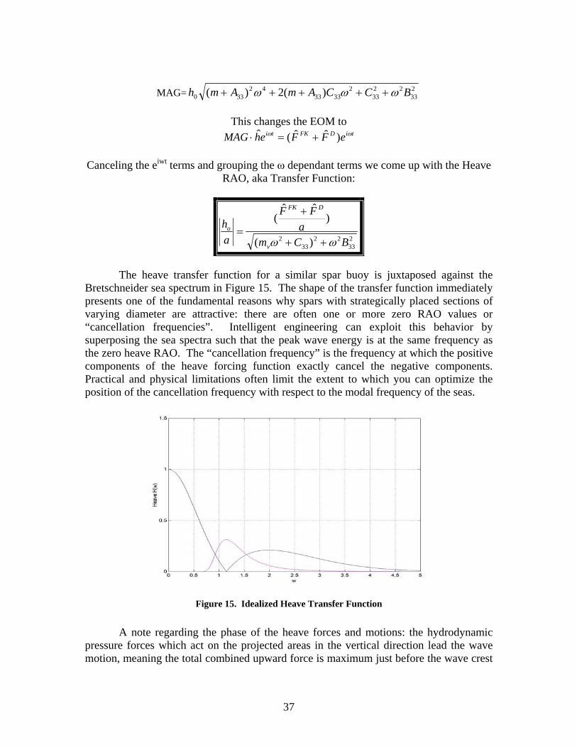
MAG= 2

3322

332

333342

330 )(2)( BCCAmAmh ωωω +++++

This changes the EOM to tiDFKti eFFehMAG ωω )ˆˆ(ˆ +=⋅

Canceling the eiwt terms and grouping the ω dependant terms we come up with the Heave

RAO, aka Transfer Function:

233

2233

2 )(

)ˆˆ

(

BCma

FF

ah

v

DFK

o

ωω ++

+

=

The heave transfer function for a similar spar buoy is juxtaposed against the

Bretschneider sea spectrum in Figure 15. The shape of the transfer function immediately presents one of the fundamental reasons why spars with strategically placed sections of varying diameter are attractive: there are often one or more zero RAO values or “cancellation frequencies”. Intelligent engineering can exploit this behavior by superposing the sea spectra such that the peak wave energy is at the same frequency as the zero heave RAO. The “cancellation frequency” is the frequency at which the positive components of the heave forcing function exactly cancel the negative components. Practical and physical limitations often limit the extent to which you can optimize the position of the cancellation frequency with respect to the modal frequency of the seas.

Figure 15. Idealized Heave Transfer Function

A note regarding the phase of the heave forces and motions: the hydrodynamic

pressure forces which act on the projected areas in the vertical direction lead the wave motion, meaning the total combined upward force is maximum just before the wave crest

37

reaches the buoy. However, the actual heave motion lags both the forces and the waves. [11]

)()()( 2 ωωω inputoutput SHS = Once the wave spectrum and the heave transfer function are fully defined, the

Wiener-Khinchine Relation (seen above) can be employed to determine the spectrum of the heave response. This spectrum shows the buoy heave response in meters at a particular frequency during a storm event corresponding to the sea state modeled by the Bretschneider Spectrum.

3.2.2.2 Implementation and Results From the beginning of the design process, all analytical exercises were completed

using computational/mathematical software. Both Matlab and MathCAD were employed extensively to help ease the iterative nature of naval architectural design. The heave analysis was done using a script which was written for Matlab. The buoy and metrological/oceanographic conditions were modeled as closely as possible, and then, employing the theory outlined above, heave estimates were generated. This Matlab script was an effective tool in rapidly evaluating various design modifications and geometries.

The script was used as a design tool and to estimate the heave response in a given sea state. Although velocity and acceleration predictions are less important in heave than in roll for this application, they were included in the Matlab analysis. The figures and table below outline the heave estimate behavior and magnitude. The significant heave response amplitude shown in Table 7 below, 0.124m, is well below the design constraint of 50cm.

Figure 16. Actual Heave Transfer Function for the Final Design

38

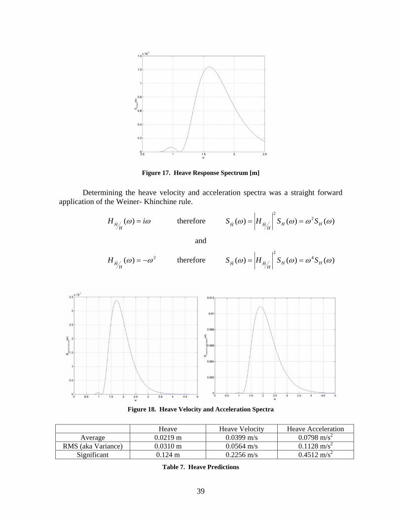
Figure 17. Heave Response Spectrum [m]

Determining the heave velocity and acceleration spectra was a straight forward

application of the Weiner- Khinchine rule.

ωω iHH

H =)(& therefore )()()( 22

ωωωω HHH

HH SSHS == &&

and

2)( ωω −=H

HH && therefore )()()( 42

ωωωω HHH

HH SSHS == &&&&

Figure 18. Heave Velocity and Acceleration Spectra

Heave Heave Velocity Heave Acceleration

Average 0.0219 m 0.0399 m/s 0.0798 m/s2

RMS (aka Variance) 0.0310 m 0.0564 m/s 0.1128 m/s2

Significant 0.124 m 0.2256 m/s 0.4512 m/s2

Table 7. Heave Predictions

39

3.2.2.3 Parametric Heave Study It was important to establish an early and complete understanding of the behavior

of spar buoys with varying design characteristics. Draft, tank diameter, diameter ratios, and length all play significant roles in generating heave, roll and hydrostatic response predictions. Acquiring a qualitative understanding of the trends and sensitivities of these characteristics is known as a parametric study and is employed often in Naval Architecture. After generating the model and implementing it in a set of Matlab simulations, completing a study of the change in heave RAO with respect to varying different parameters is much simplified. All that is required is to change the input values to the model and run the simulations. Immediately, you have an idea for how these varying parameters effect the significant and RMS heave estimates as well as the natural period.

The initial study was done using a very basic spar buoy design with only two different sections. The first longer section had the smaller diameter (b) and pierced the surface. The second section was located well below the water line and had a much larger diameter (B). The procedure was basically to vary the ratio of the larger diameter to the smaller diameter for a given draft and then graph the RMS heave value. Figure 19 shows the trend.

Diameter Ratio to RMS h

0.030.040.050.060.070.080.090.1

0.11

1.00 1.50 2.00 2.50 3.00

B/b Ratio

RMS

heav

e, m

Figure 19. Parametric Heave Analysis

3.2.3 Roll Analysis

The roll response of the NEC Spar Buoy is a very important issue. Emphasizing the idea that the entire existence of the buoy is to support its scientific and communications mission, the buoy can only effectively serve as a platform for high bandwidth radio telemetry if its overall roll amplitudes and rates are minimized with respect to the surface of the surrounding sea. In the paper published by DOT on the DEOS project involving WHOI [8], the effects of buoy motions on communications efficiencies were analyzed. Table 7 is taken directly from this paper and outlines their efficiency predictions for a 5m discus buoy and 40m spar buoy. Communication “efficiency” is defined here as the percentage of time that the antenna is able to remain locked on for high-speed data transfer. The estimates were made using motions

40

predictions from Dr. Paulling’s MLTSIM software and the technical specifications provided for a C-Band antenna systems engineered by Harris Electronics Co.

Location Communication Efficiency Discus Buoy Spar Buoy

Pacifict Coast (32˚N) 55% 99% Atlantic Coast (25.6˚N) 56% 99%

North Atlantic 29% 88% North Pacific 22% 85%

Worldwide Average 48% 97%

Table 8. Predicted Communication Efficiencies [8]

3.2.3.1 Theory Deriving the coefficients integral to the roll transfer function and understanding

the added roll inertia are both difficult aspects to the roll analysis. There are four important coefficients in the roll equation derived by Berteaux, shown below. In his original technical paper written at WHOI for ONR back in 1977 [3], there is an explanation on how to estimate these coefficients.

Figure 20 is a generalized drawing of the type of spar buoy modeled in this roll analysis. Obviously, the major parameters are draft lengths, diameters, and the center of gravity.

Figure 20. Roll Body Diagram

2

2

dtdIM v

ii

θ=∑

where Mi represents all external moments exerted on the buoy, and Iv is the virtual moment of inertia including both physical and hydrodynamic components.

r1

r2

h3

h2

h4, KG

d1

h1 , S

d2

d3

d4

41

222

222 )()()(

ωωθωDPkC

AH Roll

+−⋅==

)()( ωω BIC v +−

The above equation is the generalized form for the Roll transfer function. The coefficients are defined by

Using W p integrate Berteaux’s explanation of these coeffic i ame up with the following equations.

- ‘C’ represents the roll stiffness in units of righting moment per degree - ‘P’ represents the wave inertia - ‘D’ represents the wave drag

ping - ‘B’ represents the buoy roll dam toHOI aper 77-12 [3], I was able

ients w th our particular buoy design and cReference Figure 20 when necessary. The initial, integral form of each of these coefficients is taken directly from Ref [3].

Coefficient of Buoy Roll Damping: ⎧ =Sr

⎪⎭

⎪⎬⎫

⎩

⎪==

==

KGr

rr

B2

2

1

1 02

0

⎪⎨ + ∫∫ drrrddrrrd 3

2213

11 )()(αω

Θ= DCρπ

α34

Θwhere is an estimated average roll amplitude and was assumed to be 1° which is within 0.1° of the estim ted RMS value. a

For our buoy:

))()((3

43

444

433

4222

4411 hhdhdhdhhdCB D −+++−Θ= ρ

πω

Coefficient of Wave Drag Moment:

=== r

kr

r

dreD2

2

1 0222

0111β

⎪⎭

⎪⎬⎫

⎪⎩

⎪⎨⎧

− ∫∫=

−=

−−KGrSr

krkS errddrerrd21

1 222 )()(

ωρπ

β FD AC34

=

where AF hat is the estimated average value of fluid particle motion amplitude and is assumed to be roughly one half the average wave height

For our buoy:

[ ] [ ]{ }14

=k

D

Coefficient of Wave Inertia Moment:

)12()12()12( 22

22

12

12

2221

1

+−+−−−⋅ −

khedkhekhede khkhkhkhβ

2

=== rr

dreP2

2

1 02

0

γ ⎪⎭

⎪⎬⎫

⎪⎩

⎪⎨⎧

−− ∫∫=

−=

−KGr

krSr

krkS errddrerrd21

12

2211

21 )()(

42

ρπγ mC4

=

Where Cm is the added mass coefficient of a Cylinder in normal flow, 1.2

For our buoy:

⎪⎪⎭

⎪⎪⎬

⎫

⎪⎪⎩

⎪⎪⎨

⎧

⎥⎦⎤

⎢⎣⎡

⎥⎦⎢⎣⎥⎦⎢⎣⎥⎦⎢⎣

+−

−+−

+

=

)14(4)13(324

3322121

2kh

khekh

khed

d

kP

γ

It is interesting to see how these damping coefficients change with frequency. Figure 21 illustrates these trends.

⎤⎡⎤⎡⎤⎡ +−

−+−−−−− )1(312)1(212)1(1)1(22 khkh

edkhkh

edkhkh

ekhkh

e +

Figure 21. Roll Coefficients

3.2.3.2 Implementation and Results A Matlab script similar t heave analysis was written for

the roll analysis. Both of these scripts can be found in the appendices to this thesis. The theory outlined in the preceding chapter is represented in the code and implemented to analyze the final NEC Buoy configuration. The angular motion and velocity must be at

o that used to automate the

43

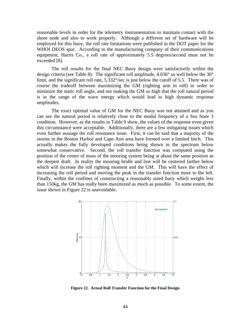
reasonable levels in order for the telemetry instrumentation to maintain contact with the shore n

atic roll angle, and not making the GM so high that the roll natural period is in t

ssuage the roll resonance issue. First, it can be said that a majority of the storms

ode and also to work properly. Although a different set of hardware will be employed for this buoy, the roll rate limitations were published in the DOT paper for the WHOI DEOS spar. According to the manufacturing company of their communications equipment, Harris Co., a roll rate of approximately 5.5 degrees/second must not be exceeded [8].

The roll results for the final NEC Buoy design were satisfactorily within the design criteria (see Table 8). The significant roll amplitude, 4.036° us well below the 30° limit, and the significant roll rate, 5.332°/sec is just below the cutoff of 5.5. There was of course the tradeoff between maximizing the GM (righting arm in roll) in order to minimize the st

he range of the wave energy which would lead to high dynamic response amplitudes.

The exact optimal value of GM for the NEC Buoy was not attained and as you can see the natural period is relatively close to the modal frequency of a Sea State 3 condition. However, as the results in Table 9 show, the values of the response even given this circumstance were acceptable. Additionally, there are a few mitigating issues which even further a

in the Boston Harbor and Cape Ann area have formed over a limited fetch. This actually makes the fully developed conditions being shown in the spectrum below somewhat conservative. Second, the roll transfer function was computed using the position of the center of mass of the mooring system being at about the same position as the deepest draft. In reality the mooring bridle and line will be centered farther below which will increase the roll righting moment and the GM. This will have the effect of increasing the roll period and moving the peak in the transfer function more to the left. Finally, within the confines of constructing a reasonably sized buoy which weighs less than 150kg, the GM has really been maximized as much as possible. To some extent, the issue shown in Figure 22 is unavoidable.

Figure 22. Actual Roll Transfer Function for the Final Design

44

Figure 23. Roll Response Spectrum [m]

Determining the roll velocity and acceleration spectra was, again, a straight

forward application of the Weiner- Khinchine rule.

Figure 24. Roll Velocity and Acceleration Spectra

All of these spectra show the mnatural frequency in roll w ll frequency should have been somewhere less than that at around 1 rad/sec or less. This would correspond to a

io as well. Roll Roll Velocity Roll Acceleration

aximum response to occur at roughly the buoy’s hich is 1.31 rad/sec. Ideally, the ro

roll period of 6.3 seconds and would be well to the left of the sea spectrum peak and outside the danger zone in the developing seas scenar

Average 0.71 deg 0.94 deg/s 1.26 deg/s2

RMS (Variance) 1.009 deg 1.333 deg/s 1.781 deg/s2

Significant 4.036 deg 5.332 deg/s 7.124 deg/s2

Table 9. Roll Predictions

45

3.2.4 Developing Seas Issue When a storm or sea state is developing, the ocean does not instantaneously go

from its placid state to 2 meter waves of 5 second period. There is of course a transitional state associated with this process called “developing seas”. During this period, as a storm forms or moves in, the equilibrium characteristics of the seas slowly transform; the high frequency, broad spectrum, low amplitude chop that characterizes an impending storm eventually fully develops into the large/peak amplitude waves associated with the storm event.[14] If you were to plot wave spectra based on the significant wave height and average period at different points in time leading up to a storm event, you would see them moving in from the right hand side of the frequency axis see Figure 25). tructure such that its natural frequency of o aph) of the maximum sea spe

( For this reason, it is smart to design your sscillation is below that (or to the left on the gr

ctrum, thereby it can take less energy from the “developing seas”.

Figure 25. Representative Developing Sea Spectra

3.3 Mooring design

Mooring systems have gained increasing importance in the overall design phase in recent years. This is because in deep-water, stationary facilities the mooring system might account for a significantly large (and growing) percentage of the total value/cost of the project. Also, failures in a mooring arrangement can result in much more catastrophic and costly losses or damages than elsewhere on the hull. With buoy systems, mooring design tends to be governed by an entirely different (while related) set of environmental criteria than the hull. Mooring design is much more sensitive to the current and submerged conditions while the overall motions of the hull are largely dictated by the wind and wave conditions which operate on a much smaller scale. [12]

Although some buoy systems, spars in particular, can be allowed to freely float on the ocean surface (they are called “drifters”), the inherent nature of the NEC Buoy mission requires some degree of station keeping. With some communications and navigation type objectives, having a dynamically positioned buoy with the ability to keep its “station” is a necessity. This type of dynamically ‘moored’ buoy will be explored later in this thesis with respect to the GIB system. However, for the NEC buoy exact

46

stationkeeping and time-dependant mobility was not a requirement, so the conventional methods of mooring a spar buoy were explored.

In general mooring a small (less than 10m) spar buoy is somewhat difficult given their propensity for having limited reserve buoyancy. These difficulties can be avoided in a number of different ways, the most obvious being to design the mooring line and chain such that it is as close to neutrally buoyant as possible; therefore it exerts no downward force on the buoy. [2] There are two types of mooring systems employed for buoys: slack and taut moorings. These names are relatively self explanatory but the advantages and disadvantages of each are not. Slack moorings require more line length which means a greater mooring weight. In this scenario, the line, chain, shackles etc. hang under their own ancy of the buoy to

ooring weight, uoy offset, buoy displacement to weight ratio, and buoy dynamics. The tension is also

nd tide forces. Dependant upon the location at which the wnward force exerted on the buoy by the mooring line can

either ameliorate or make worse the heave and pitch response amplitudes. As with any moorin

3.3.1

considerable currents, there are also considerable drag forces which increase lin

weight relying on the reserve positive buoymooring is dependant on the msupport them. The tension in this type of

bdependant upon the current amooring is connected, the do

g, in order to least influence the motion of the buoy with the mooring tension, the point of attachment should be roughly around the submerged center of effort.

Taut mooring designs are used on buoys with excess buoyancy and greatly effect the dynamics of the system. These types of mooring lines are generally made of stronger materials than their slack counterpart because of higher static and cyclic loading/stresses. In the offshore industry, taut moorings often have failure problems with the high frequency (getting higher with increased depth and line tension) loading on nodal points like shackles and fairleads.

Line Dynamics The static analysis of mooring lines and cables is well understood and

documented. The math involved in this analysis has been transferred into simulators and codes which invoke them in their numerical form. The theory behind cable analysis is based on the summation of forces, from current drag, gravity, and line tension, on incremental pieces of line. When there are not considerable currents at the site, as is the case for the NEC buoy, the tension at a point on the line should simply be equal to the weight of the line below it. When there are

e tension. Using the force summation method, one can estimate the motion or geometry of the flexible line along its length.

In order to give a brief introduction to cable analysis as it applies to floating buoys and thus this research, the basic two-dimensional approach is outlined here. First, the line itself is broken up into representative, incremental elements, and it is assumed that each mooring element has a static vector force balance. In the vertical direction there are buoyancy, tensions from above, tensions from below, and the vertical drag component. In the horizontal direction the forces are given by the angled tension from above and below, and the horizontal drag component. Each element acts dynamically as a “hinge” even though it is “rigid” in reality. For each of these line elements there are three equations and six unknowns. [22]

47

111 sincossincos +++=+ iiiiiixi TTQ ψθψθ

111 sinsinsinsin +++=+ iiiiiiyi TTQ ψθψθ

coscos =++ TTQgB 11 ++ iiiizii ψψ

Variable Definitions:

Figure 26. Line Segment Definition

- Ti and Ti+1 are the tension above and below the element, respectively

- Bi is the buoyancy at the present element

- Qxi, Qyi, and Qzi are the drag forces in each direction

- ψi and ψi+1 are the spherical angles from the vertical from the tension above and below, respectively

- θi and θi+1 are the spherical angels in the x-y plane from the tension above and below, respectively

The positions of each mooring element relative to a fixed point, often the anchor, can be determined and then summed successively up the line.

iiiii LXX ψθ sincos1 += +

iiiii LYY ψθ sinsin1 += +

iiii LZZ ψcos1 += +

3.3.2 Matlab Simulation The evaluation of the Reynolds number is important in the mooring analysis

because it allows us to approximate the drag coefficient on the line or cable. The Reynolds number remains subcritical (<3x105) for the range of current velocities seen by the buoy mooring line (see Figure 27). For subcritical Reynolds regimes, the drag coefficient of the line is approximated as 1.2. Obviously the accuracy of the position and

Ti

ψi Z

ψi+1Y

Y

Z

θi

Ti+1θi+1

X

X

48

am ten, engineers will run Monte Carlo simu efficients, run the dynamic analysis of the m random values and then statistically analyze the results.

plitude of the buoy offset is dependent on the drag coefficient. Oflations to generate random drag co

ooring system for each of the

-50

-40

-30

-20

-10

00 500 1000 1500 2000 00

Dep

th [

25

m]

-60

-70

Reynolds Number

Figure 27. Reynolds Number for the Given Current Profile and 5/8” Line

to 300m of 5/8” Nylon line with a (conservative) specific gravity of 1.2 which corresp

actual density of Nylon is 1100 kg/m , s.g. 1.073. The conservative specific gravity allows for the use of larger diameter line if needed or conveniently available. The buoy will never likely be moored in that deep of water. A more probable depth range would be 80-100 meters of water. An alternative mooring material, if the weight of the line were to be an issue, would be polypropylene which is neutrally buoyant but also more expensive.

The mooring analysis tool mdd.mat (explained earlier) was employed to t of the buoy for the current profile as defined by the

GoMO

hile lower ratios (i.e. smaller line lengths) were allowable with the polypropylene line. The results from this analysis are outlined in Figures 28, 29 and Table 10 below. Figure 28 shows the result for a neutrally buoyant line material (polypropylene). The remaining results are for the 5/8” Nylon design line. It appears

The NEC buoy mooring was designed for a maximum mooring weight equivalent

onds to a density of 1230 kg/m3. This corresponds to a maximum in air weight of15.85kg; see Appendix 3 for a full description of the mooring weight estimates. The

3

determine the approximate offseOS Data Buoy 44029. This tool was also used to analyze the DEOS Spar mooring

designed for WHOI by DOT. The mooring configuration was analyzed for varying ratios of mooring line length to total water depth (L/H). The water depth at the GoMOOS 44029 location is approximately 62m. The mooring simulation was run with:

- 150m and 300m of Nylon line

- 85m and 150m of Polypropylene line

Analyses completed with line L/H ratios of 2 or less with the Nylon line caused the program to fail, w

49

that the current is so benign that the buoy just displaces in the direction of the current by the slack in the line.

Figure 28. Buoy and Mooring Offset for L/H ratio 1.3 with Polypropylene Line

Figure 29. Buoy and Mooring Offset for L/H Ratio 2.4 and Nylon Line

150m Line 300m Line Float Model 23 kg positive sphere 23 kg positive sphere

Shackle 5/8” 5/8” Line 5/8” Nylon 5/8” Nylon

Anchor 2 concrete blocks 2 concrete blocks %Buoyancy used 14% 20%

50

Tension at Anchor 1.8 kg 3.5 kg Vertical Load -1.4 kg -3.3 kg

Horizontal Load 1.2 kg 1.2 kg Safe Wet Anchor mass 1 kg 1.9 kg

Safe dry steel anchor mass 1.1 kg 2.2 kg Safe dry concrete anchor mass 1.5 kg 2.9 kg

Table 10. Mooring Simulation Models and Results

3.4 Structural Design

Spend one night aboard a ship or ocean structure, lay still and listen to the creaks and moaning of the, often, large steel hull, and you immediately gain an appreciation for the types of loading that must be withstood at sea. Just as important as meeting the mission requirements and mitigating dynamic responses, the structural design of an ocean system must be completed with care and redundancy. With less complex systems, the problem is as simcondition

The hydrostatic pressures and body forces on a hull are generally straight forward. There is an everywhere normal pressure force which is proportional to the height of the water column above the structural element. There is also the gravity loading of the structural and payload constituents themselves. Dynamically, however, estimating the forces on a moving, or static, hull from a never static seaway is rarely 100% accurate. Inertial forces are balanced with forces and are highly dependant on the systems and the Reynolds number regime at any given time. Even with computationally expensive and trusted analyses, ignoring or taking for granted the effect of cyclic loading on the life of a structure can be fatal. Fatigue and corrosion failures are common in the marine environment and some types of structures, especially in taut mooring designs on deep-water, high-pretension installations.

Given the fact that building a prototype (mini spar-buoy) for load testing is out of the question, we have but one chance to generate sufficiently accurate stress predictions and design within a factor of safety – one which is both conservative from a failure stand point and acceptable from the cost perspective. This will hopefully be accomplished by using the FEA tool associated with the Solid Works CAD package called Cosmos. Using Cosmos, a detailed estimate for the stress concentrations, deformation amplitudes, and minimum saf

As with most marine systems, re ize and purpose, most intense lo ur during laun en, at the the life of the system, dynamic, static, and lled “jerk” loads are m m. For example, once installed, the buoy will pr r be pivoted on a single point in its structure alo ide – as if it were b he side of a b

ple as calculating the stresses and deformations to an easily defined load . With a marine system, however, the loading is all but easily defined.

ety factors can be analyzed for a variety of loading states.

gardless of s some of the ad cases occ ch and recovery. Oft se transition points in

so ca aximuobably neve

ng the s eing pulled over t oat.

51

3.4.the new des ble to employ readily ble and

e order to ma he schedule. Of cours lighter materials to construc s was favorable for ydrostatics, but issues of strength and durability discourage their use and almost

the use of a metal. The structure could have been almost entirely made of bout cracking and wear due to salt water exposure and efits of a much lighter and somewhat cheaper structure.

1 Materials It was important that

asily machinable materials inign be a availaintain t e using

t the main buoyant pipe and the lower platehnecessitatedPVC and Delrin, but concerns a

V radiation outweighed the benU

The final decision was to use Aluminum to construct the buoy structure. Al alloy 6061 is most commonly used because it’s strong, easily machinable, and has good corrosion resistance. Its popularity was thought to make it more easily available and potentially cheaper. Table 11 outlines the fundamental characteristics of Aluminum 6061.

Aluminum Alloy 6061 Poisson’s Ration 0.33

Yield Strength 5.5x107 N/m2 Elastic Modulus 6.9x1010 N/m2

Tensile Strength 1.24x108 N/m2 Sheer Modulus 2.6x1010 N/m2

Mass Density 2700 kg/m3 Specific Heat 1300 J/(kgK)

Table 11. Buoy Material Properties

3.4.2 COSMOS Analysis COSMOS is the finite element analysis tool which accompanies the Solid Works

CAD software package. COSMOS has the ability to analyze solid models (parts and assemblies) for stress and strain distributions, overall displacements, and check the design for minimal factor of safety. This is an excellent tool for a design project like this one where there is no plan of prototype manufacturing.

ge water depth, hydrost

e was generated by fixing in space the top of the buoys main spar g gravity. The battery weight was also added at the location of the

battery

In trying to decide which load conditions to analyze, only two were chosen. Both are static load scenarios which correspond to a “not-so-bad” deployment situation where the buoy is being held under its own weight and the second corresponds to a more severe situation where the buoy is being pulled over the side of the boat and is hanging (approximately) like a cantilever beam. The second loading case is the most conservative static loading case that was identified. No dynamic loading scenarios were analyzed, and because the deepest draft was really nothing compared to the avera

atic pressure loading on the aluminum tubulars was also not analyzed. It was assumed that the pipe sections were more than strong enough to withstand this small pressure force.

3.4.2.1 Load Case 1: Hanging Vertically Under Gravity This load cas

section, then applyin can, although they were not modeled. The results of this analysis show that the

system is more than sufficiently strong enough to withstand basic gravity loading. Table 12 and Figure 30 outline the results of this analysis.

52

Type Minimum Maximum Safety Factor

Displacement 0 m 3.78e-5 m N/A

Von Mises Stress 2.91 N/m2 1.63e6 N/m2 33.7

Table 12. Load Case #1 Results

Figure 30. Stress and Deformation Plots for Load Case #1

3.4.2.2 Load Case 2: Pin-Free Bending Model This load case was generated by adding a small flat face to the top side of the

upper pipe section. This face was fixed and then both gravity and the battery load were e long axis of the buoy. ing present if we were to

pull the

added to the buoy structure in a perpendicular direction to thAgain, this was supposed to simulate the worst-case static load

buoy out of the water by resting it on the rail of the boat. Table 13 outlines the results of this analysis.

Type Minimum Maximum Safety Factor

Dis nt placeme 0 m 0.025 m N/A

V 9.5 N/m2 3.65e6 N/m2 15.1 on Mises Stress

Table 13. Load Case #2 Results

53

As with most of the naval architecture that is done within the world of pure ocean engineering, the system being designed will exist solely to accommodate some sort of ocean science and/or technology. For the NEC buoy this science includes the acoustic communication of an underwater robot with a moored buoy and surface telemetry.

Part of what gives this design project value and makes it interesting are the seakeeping requirements generated by the motion sensitive payload and its intended location of deployment. The factors which force certain draft and dynamic response limitations are directly linked to the fact that the buoy must operate in the Cape Ann area of the Northern Atlantic Ocean. Furthermore, this requirement is directly linked to the scientific and communications mission of the payload. Therefore every detail of the design can be traced back to the mission of the payload.

The electronic components which comprise the payload also have performance characteristics which favor certain design types. For example, low roll [angular] velocities or consistent antenna to shore contact –which can be threatened by exaggerated heave responses- might be conducive to the radio telemetry or GPS instrumentation on board. The actua explained in the

is. In summary, this buoy is to facilitate the operation of communications system which maintains contact with an on-shore antenna, establishes

es a link for acoustic transmissions ission implies the use of a WAN

card an

3.5 Electronic Systems Outline

l mission of this particular buoy was thoroughly introductory portion of this thesaa localized wireless area network (WAN), and providfrom underwater vehicles to ships and shore. This m

d amplifier circuit, a centralized computer with memory space, an antenna and mast set-up, an acoustic modem and associated transducer, and of course, a power system capable of supporting all of this instrumentation. Figure 31 shows this system in schematic form.

54

PC104 Stack and Peripherals :

- Computer - Memory - Power Conditioning - Inertial Navigation System

WAN Electronics: - 802.11 b Card - Amplifier Circuit - GPS

Battery Can:

- Batteries - Solar PanelCharge Circuitry

Acoustic Comms :

-Micro-Modem board - PWR amplifier circuit - 1.2 GB flash card - 8 channel A2D card

8dbi Antenna

Analog Signal

Optional Topside B

attery Charging C

able/Connector

PWR

Transducer

PWR

Data

PWR Out ( 12 V )

Data

Solar Panels

PWR

PWR(if needed) External Sensing

Packages

- Temperature - Wind Speed - NEREUS Hydrolab

** Optional **

Data

Extra Connectors

Figure 31. NEC Buoy System Schematic

3.5.1 Power System A potentially heavy and cumbersome power system was anticipated from the

beginning. In its ideal operational state, the buoy would be responsive and available for

55

both acoustic and radio communications at all times of the day. The transducer for the acoustic modem alone can draw up to 30 Watts when in use. The additional power draw of the other instrumentation could drain a conventional 12V power source in under a day. This kind of endurance timeframe is simply unacceptable on a system which is deployed in generally inhospitable waters and on which the batteries will probably be located well below the DWL for hydrostatic purposes. Identifying an operationally and financially plausible power supply for the NEC buoy project was very challenging. The fundamental pieces of information required to select a power system are the anticipated duty cycle, voltage required, and power draw in Watts. In most cases these values won’t be entirely uniform or consistent throughout the system, and so an average value is estimated and employed in the calculations.

The term ‘duty cycle’ refers to the ratio or percentage of time a component or system is in use. Initially a 24hr/day duty cycle was desired, but given the unreasonable demands this would generate on a battery system, an 8hr/day, or 33% duty cycle, was established as much more reasonable. Given the deployed environment and inconvenience of frequent battery replacements or changes, the buoy would ideally be able to operate autonomously for approximately 30 days. Therefore an 8 hr/day, 30 day (240hrs) endurance specification was imposed on the power system options.

All but one of the payload components require much less than 5W of power to operate. Table 13 shows the power estimates broken down by instrument. The Micro-modem transducer is the only thing which requires more than 5W. Assuming that the transducer is employed only a fraction of the day, it is safe and conservative to use 7W average power draw for the overall system. In addition to the intended power draw, the average voltage required by the electronic instrumentation is set at 12V. Table 14 also outlines the actual voltage rating for each component.

Part Supply Voltage Max. Power Standby Power Average Power

V W W W PC104 CPU 5 1.6 0.2 0.9 Flash Card 5 0.17 0.0025 0.08625

802.11b radio 5 3 1 2 PCMCIA card 5 0.35 0.35 0.35

Serial card 5 1 0.5 0.75 GPS Receiver 12 0.575 0.575 0.575 Micromodem 12 30 0.2 3

Totals 36.695 2.8275 7.66125

Ta t

.5.1.1 Battery Selection Given the assumed power draw (7W), duty cycle (8 hr/day), and voltage required

system is now transformed into a task of matching and

ble 14. Power Consumption by Instrumen

3

(12V), choosing a battery optimization. Batteries are generally described in Amp-Hours at a set voltage. Obviously for our purposes (240hr * 7W) 1680 Wh at 12V (or 140 Ah) is necessary. The optimization is required to find the cheapest battery option, or combination there of,

56

which provides 1680 Wh at 12V while not exceeding a reasonable weight and size limitation. In this case, because the buoy itself was not to exceed approximately 150 Kg and be manageable by a small research vessel without an A-frame, the power system was limited to ~50kg and need needed to fit in the 12” Al pipe that was eventually employed by the structure.

The final power source selection was narrowed down to one of the easily available sealed Sea Volt AGM batteries sold by West Marine. These batteries are intended for marine applications, are rugged, can be oriented in any position, and are relatively cheap while providing a decent energy density. One of the unfortunate characteristics of these batteries is that they’re rather large, where even the smallest option would require 12” pipe. The final choice was to employ one of the 105 Ah batterie

3.5.1.2

FLEX 5©, produce approximately 175 Wh power per week (assuming 4-5 hours of average daily peak sunlight). Using this estimate, the solar panels could potentially contri nother ow er hprovide another 35 days of operation, that’s not accounting for the additional power ge e sun in tho additional day his extension robably unreas ble to ex c udy, rainy/sno nditions o ea, 4-5 hours of peak sunlight is highly unlikely. A more conservative estimate is say a quarter of that which w the power estimate to ~43 al 9 days. Again, the behavior and performance of solar panels in the type of environment they will be used here has not been explored, so these estima off base.

3.5.2 W OI Micro-Modem oods Hole Oceanographic In n (WHOI) is one of the wor ier

“brain trusts” when it c n exact compliment to HOI employs, there also exists an expert team of ocean

se men and women, often trained through the WHOI-MIT joint pr

s (31.7 kg). This battery would only allow 22.5 days at the assumed duty cycle but this was considered sufficient for now. The next option up, 200Ah, would afford the 140 Ah requirement however it would require a pressure vessel –or battery canister- with a 13.12” ID, and without expensive and time consuming machining, one of these is not available. In the future, if more funding for a power system retrofit is available, a more energy dense battery pack with more suitable dimensions should be researched.

Solar Panels In part because increasing the power endurance of the buoy is desirable, and in

part because their performance in the wintry North Atlantic is poorly characterized, solar panels will also be present on the NEC Buoy. West Marine sells an array of solar panel products. They also sell wind generators, typically for sail boat use, but these were determined to be too inefficient for the structural burden they would imply and thus ignored. In an ideal situation, the solar panels which were selected, the BatterySAVER

bute a 125 Ah to the p er system ov 60 days. 125 A at 12V would

nerated by th se s. T is p onapect. Given the grey, lo wy co f the ar

ould decrease Wh/wk or an addition

tes might be completely

HThe W stitutio ld’s prem

omes to ocean science and exploration. Ithe core of oceanographers that Wphysicist and engineers. The

ogram, help develop the hardware and processes which facilitate the work of the scientist and explorers. In recent years, WHOI has developed its own stand-alone acoustic modem package, which is called the Micro-Modem. This device will be employed on the NEC buoy.

57

In actuality, the Micro-Modem can be used for more than just underwater acoustic communications. The creators of Micro-Modem envisioned a much more versatile combination of hardware and software which can be employed as an acoustic navigation beacon, a passive navigation device, a nodal point in an acoustic network, or a UAM (underwater acoustic modem). The motherboard hosts a TI TMS320C5410 DSP, a hi-speed 1

computer because it is essentially a PC with a different form factor w

the wireless nna were also installed on the buoy. The unit is a

y. At the lowest level, the hardware itself is outfitted with

2 bit Analog to Digital (A2D) converter, flash memory, a low rate A2D, a real time clock, and other peripherals. All electronic hardware is designed to fit inside a 2 inch inner diameter pressure vessel. They rely on a set of Lithium-Ion batteries and a power amplifier. All of these components are a relatively low power draw except for the power amplifier for the transducer which draws up to 30 Watts when in use. [15]

3.5.3 Computer As with most of the projects that are realized here at MIT Sea Grant, the NEC

buoy will employ a PC104 programmable computer. This centralized computer will talk to all the communications and power hardware using code patched together from similar projects. The PC104 gets its name from the first personal computers designed by IBM, the “PC”, combined with the number of pins used to connect the cards together (104). It was developed in the late 1980s by Ampro Computers of California. The PC104 is the quintessential embedded

hich meets reduced signal drive and power requirements. These systems are used virtually anywhere a device must be controlled by a programmable computer; the MIT Odyssey class AUV employs the PC104.

The PC104 stack used in the NEC Buoy is shaped like a rectangular prism (4”x4”x8”). The stack “cage” is mounted under the topside end-cap. A 6-pin bulkhead connector and two coax connectors are mounted to the end-cap and join the stack with the submerged battery can and the antennas mounted above on the grab bar.

3.5.4 Hardware The wireless network hardware consists of an 802.11b wireless Ethernet card

incorporated into the PC104 stack, and an antenna. The wireless hardware selected for this project consists of a Senao "SL-2511CD PLUS" 200mW PCMCIA card and a Hyperlink Technologies 5dbi omni directional antenna. For testing in the Charles River antennas were simply mounted to the grab bar. When the buoy is deployed in the open ocean they will be connected to the top of a 5ft antenna mast.

It is important to mention that for general purposes as well as to test hardware, a GPS system and anteTrimble Lassen LP 8-channel DGPS-capable receiver, hosted on a Parvus OrbiTrak PC/104 module.

3.6 Communications Software Overview As with most systems, the software utilized for the NEC Buoy application can be

described in a hierarchical wa

58

some “

to the Linux kernel is a TCP/IP module which has three main “socket

firmware” which refers to embedded code which cannot be changed and allows the device to function properly. Above that is the basic Linux operating system which acts as the user interface to all higher level code. Above the Linux OS there are two types of drivers, the Linux kernel modules and the user space drivers. The Linux kernel hosts the kernel modules while the user space drivers are external to the kernel.

One of the important kernel modules incorporated into the software for this project is called “hostap” which allows the 802.11b card to communicate with the CPU and the other hardware connected to it. “Hostap” was written specifically for Linux and is freely shared via the internet by its author in Finland. A windows based 802.11b driver is supplied by the card manufacturer but was not required.

Also loaded ins” which can all communicate with each other. The first socket serves the “loop

back” function and allows drivers which are communicating with hardware on the PC104 bus via the serial kernel module to “report back”, so to speak, to the TCP/IP card. It also allows the MOOSDB to communicate and get information from other MOOS drivers which are communicating through the serial module. MOOS is a series of drivers written by the MIT Sea Grant AUV lab for marine robotics applications. The other two sockets support sending whatever information was looped back through a hardwired Ethernet connection or a wireless LAN connection. Both the inertial navigation system used to track the buoy motions and the GPS receiver are connected to the PC104 bus via a serial connection, and thus the serial, TCP/IP, and hostap kernel modules are all very important to the success of the buoy. Figure 32 attempts to illustrate the interconnectivity of the hardware via the various software components.

CPU

ISA/PC104bus

Orbitrak GPS card

INS

GPS Receiver

(Serial Ports)

802.11bCard

TCP/IP:LO

ethØwlanØLinux Kernel

5dbi antenna

'hostap' moduleSerial

Module

MOOS DB

iGPS

Figure 32. Software Hierarchy

59

4. NEC Buoy Testing

Given that this buoy was built at the request and using the funding of an external agency, the NEC, its ability to meet the goals and objectives of that agency must be demons

ete the full set of tests outlined in this

4.1.1 Short Term The immediate objectives of the testing process are rather elementary. The buoy

will never have been assembled fully as a mechanical unit, nor will it ever have been fully outfitted with the power and electronic systems intended for it. For this reason, the following simple mechanical and naval-architectural successes will be observed:

- The buoy must assemble as designed using the hardware specified - The buoy should float upright and be ballasted to sit at the correct draft - There should be no leaking of water into areas where water was not intended - The buoy should exhibit reasonable dynamic behavior (roll/heave)

From an electronics hardware and software perspective, there are also some immediate objectives.

- The electronic hardware should be tested with the proposed power system to ensure compatibility and continuity

4.1.2 Long Term There are other goals in testing this buoy which transcend those outlined above

and will most likely take place on a longer time horizon. These longer term objectives are associated with the detailed technical purpose of the buoy and would include demonstrating that the buoy

- Interoperability should be demonstrated between the various electronic components

trated satisfactorily in order to deem the project a success. Accomplishing that requires testing the buoy in an array of environments, including the one it was designed for, and performing an array of tasks. These tasks range from simple, an example being can it float, to fairly complex, can it relay a command from a shore node to a submerged autonomous vehicle. The period of time required to compl

testing plan could range from a few months, if full resources at MIT Sea Grant are available, to a few years. It is expected that future graduate students will undertake some of the testing which will be discussed.

4.1 Objectives

Every testing plan must begin with objectives and goals. In the broadest sense, MIT Sea Grant is aiming to demonstrate to the Northeast Consortium that they have produced a buoy which can do that which was promised. It should be able to operate as a nodal communications instrument, operating in the ocean and transmitting data both above sea via wireless radio communications, and below sea using an acoustic modem.

60

- A functioning wireless area nlab and on the buoy in a wat

etwork should be established both on the bench in the er environment

- has a feasible user-interface, possibly one modeled after the MOOS (reference se

he broad range of testing objectives lends itself to a phased plan where goals of similar

elecinteChache

was carrying power to where it needs to be.

Figures 33-34 show the buoy being assembled at the dock. Figure 35 is of the buoy after being pulled from the water; it

e buoy’s size. The leak testing of the battery

ction 3.6 for MOOS description) system used on the MIT Sea Grant AUVs - can be polled for sensor data from a ship or shore based sending station - can communicate acoustically with a submerged vehicle and transmit that data via

its wireless area network - can be used to send commands to an AUV or other submerged device

These goals capture the essence of the end-use idea for the buoy. If a network of

buoys were to be created, as has been envisioned, all of the communications above should then be demonstrated within the network of buoys.

4.2 Testing Phases

T type and complexity are grouped and accomplished in successive order. Not

exclusively, but for the most part, each phase will be dependant on the successful completion of the phase before it. For example, if the buoy cannot be demonstrated to float upright, there is no platform on which to complete any of the communications testing.

4.2.1 Phase I This first phase of the testing addressed many of the

short term mechanical objectives outlined above and was completed in July 2004. The buoy was assembled in the lab and any missing or inappropriate hardware was ordered or replaced. The buoy was outfitted with the power and

Figure 33. Buoy Assembly: Battery Can and Section 1

tronic hardware to ensure everything fit where it was nded and could be secured. The buoy was taken to the rles River MIT Sailing Pavilion and ballasted and leak-cked. A continuity check was done to ensure the wiring

through the cable connecting the battery can and the topside electronics

gives a good sense of th-can was done in a big tank at the lab while the other

submerged sections were tested in the river.

61

Figure 34. Buoy Assembly: Section 2 Attached

Figure 35. Buoy Testing Environment

Upon first entering the buoy into the water, it was obviously over buoyant. This is consistent with the previous calculations which estimated the buoy would need

g more to float at the desired draft. In an at-sea condition, this 25kg and transducer, as well as

ipe caused the buoy to want

d to attach approximately ns testing could continue, battery with the topside

was an inertial navigation ever, because of the cable used.

AN was demonstrated at the river, the buoy was

cuss g from per ming res oving

ul at longer ranges would be easy, but there as no way of getting power to the computer anymore.

The major lessons learned in Phase I of the NEC Buoy testing were:

- The buoy is overly buoyant for the payload as is.

approximately 25kwould come from the mooring bridle and line, acoustic modemconventional ballast. In the future, I would recommend flosection. The excess buoyancy and lack of sufficient weight lowto float at a significant (almost 60 degree angle), we attempte40kg of concrete blocks to the bottom so that the communicatiobut in the process the power cable connecting the submergedelectronics was sheered.

On board, functioning, and bench tested in the lab, system meant to take roll and heave data on the river. Howsheering and also the ballast issues, this functionality was never

The basic ability of the buoy to transmit data using the Wshort range. While on the dock and during its brief stint insuccessfully transmitting a NMEA GGA (see message type disthe GPS system at the highest bit-rate possible or 11 megabit bit rate was measured by the wireless receiver. All engineers pthe communications equipment to be successf

oding the bottom 8” p

ion below) strin second. The incoent agreed that pr

w

62

- Alternate methods for improving the roll stability should be explored, including possibly flooding the lower pipe section

- Protecting the power cable from external forces must be done

4.2.2 Phases II The future testing phases may, of course, deviate from how they are written here

based on changes in resources at the MIT Sea Grant facility and/or the results of preceding phases. Phase II of the NEC Buoy e writing a user interface to be downlo This interface may be similar to the MOOS drivers used on the MIT Sea Grant AUVs. Phase II should be less dependant on the success of Phase I.

4.2.3 Phase III Phase III is rather dependant on the success of Phase I, and includes conducting

an experiment where the buoy is transmitting from various sensors. The “master” at the receiving station will poll the buoy for data from one of its sensors, i.e. the acoustic modem. Again, testing the success of varying sensor data being sent at varying ranges will be necessary.

Additionally, moving the buoy and receiving station to the design environment would provide valuable in ommunications system to operate

le buoy would be advanta

riables to be studied essage it tries to transmit is one variable. There is also the transmission range or distance and the environment. The

testing plan will includaded onto the buoys PC104 computer.

formation about the ability of the c on this buoy when it is responding more to the sea state. Moving the buoy to this

environment would also allow for the testing of the solar panels as an integrated part of the power system. The power production estimates provided by the manufacturer of the solar panels are not exactly based on North Atlantic conditions. This move would involve setting up the testing process off of the coast of Cape Ann, Massachusetts. The MIT Sea Grant Lab has relations with a commercial fishing outfit at that location and would likely be able to use their facility for this type of testing.

4.2.4 Phase IV The final foreseeable phase in the NEC Buoy testing plan would be to validate the

potential for the buoy to be used in communicating acoustically with submerged vehicles and then transmitting that data back to the receiving station. The “master” could send a data query to the AUV sensors via the buoy, or furthermore, could send a command or even mission to the AUV in this manner. One could see where a mobi

geous in this scenario. If the buoy could monitor the position of the AUV and position itself within the optimal range for acoustic communications, i.e. directly above, its usefulness and efficiency would be increased.

4.3 Test Variables

Given that the buoy as a testing platform is in a static state, the real va involve the communications system. The type of m

63

efficienis moore hesis, the operation of these types of electron arsher conditions where

operly or as efficiently.

A standard. NMEA uses printable ASCII text.

, data is transmitted in the form of a “sentence” or packet which has a comm

rt with a “$P”; for example Garmin GPS units use both NMEA standard and proprietary

cy of the wireless telemetry will be altered by the environment in which the buoy d. As discussed in Section 3 of this t

ics systems are influenced by the motions of the buoy. In hthe buoy responds more to the motion of the sea, the communications system

might not function pr

4.3.1 Message Type As with every other industry, the marine electronics industry has an agency which

establishes standards. The National Marine Electronics Association (NMEA) is a non-profit organization comprised of manufacturers, distributors, dealers, educational institutions and users of marine electronic products. The message types for the primary phases of testing will follow the NME

Using NMEAon form. They all start with a “$”, a two letter “talker ID”, a three letter

“sentence ID”, and are then followed by a number of data fields separated by commas and terminated by carriage return/line feed. A NMEA sentence may contain up to 82 characters including the “$” and CR/LF. Some marine instruments have proprietary sentences which sta

sentence types.

One of the standard sentences used with a GPS system and likely to be used as the basic message type for the Phase I testing, is the GGA or Global Positioning System Fix Data. This sentence type tells when the fix was taken, the latitude, longitude, fix quality, number of satellites, horizontal dilution of position, altitude above mean sea level, time since last DGPS update and the DGPS station ID number. Other standard NMEA sentences which might be used in the testing are DBT (depth below transducer), MTW (water temperature in Celsius), or VHW (water speed and heading).

64

5. Mobile GIB Buoy Design

The communication technologies which are being facilitated by the NEC Buoy could be used in a wide variety of applications. A few of those applications, either because of function or proponature of a buoy. For deep

sed environment, would be negatively impacted by the static

is certainl

nications system to track underwater vehicles and tra

igure 36) is a 400 kg mobile communications buoy shaped like a monohull which can operate up to seven days autonomously with its diesel generator. More recently ACSA also introduced a lower-cost, lighter-duty version of BASIL which they call MiniVAMP (Virtually Anchored Multipurpose Platform, Figure 37). This product is much better suited to the needs of the MIT AUV lab and should be evaluated further. The main potential issue with the MiniVAMP is that it can only operate autonomously for up to 8 hours. This could limit its usefulness.

water deployments, it simply would not be feasible to moor a buoy of this smaller scale. The two possible solutions to this problem are one, making the buoy much larger such that it could maintain the massive mooring system required in deep waters, or two, integrate a propulsion and station-keeping system into the design. The first option is obviously not considered because it would require expensive and complex fabrication, transport, and maintenance processes. The second idea however,

y attractive and will be discussed further in this chapter.

5.1 Existing Model

The idea of using a mobile communsfer data at sea has recently been addressed. The French organization ACSA,

Architecture et Conception de Systèmes Avancés, which is responsible for the GIB (GPS Intelligent Buoy) system has brought a mobile version of this technology to the market with the help of GEOCEAN, another French engineering company. Of course, it is expensive and not necessarily optimized for the types of operation the MIT Sea Grant AUV lab would most likely try to complete.

Their main mobile GIB product is called BASIL. BASIL (F

Figure 36. Mobile GIB Concept, BASIL [24] Figure 37. MiniVAMP Vehicle [24]

65

5.2 Potential Designs

Given that the idea of an autonomously mobile buoy with some set of onboard “intelligence” and communications capabilities is somewhat new, the understanding of which type of vessel shape is hydrodynamically and otherwise optimal does not yet exist. BASIL, the more robust and larger mobile GIB buoy is shaped like a typical v-bottom monohull. The shape and scale of this vehicle undoubtedly allows it to withstand much harsher sea environments than its smaller counterpart, the MiniVAMP. The MiniVAMPs trimaran design makes it more suitable for use as a mobile “platform” for the GIB electronics or other systems. Two other design types which could potentially work will be addressed here.

5.2.1 SWATH Type The SWATH acronym refers to a vessel type which has seen marginal popularity

Small Waterplane Area Twin Hull concept has been applied earch vessel design, and with less prevalence in the

world Navies. The basic idea is that of two submerged hulls connected to a topside deck via a s

over the past 70 years. Thesuccessfully to the fast ferry and res

trut structure. Figure 38 shows a basic SWATH design drawing taken from www.SWATH.com. Given that the slender strut members are all that pierce the water surface, the wave making resistance is decreased, which allows for faster operational speeds in more severe sea states. SWATH ships tend to have structural issues at the connection of the struts with the deck. This is the point of maximum axial stresses and near maximum shear stresses.

Figure 38. SWATH Concept

The SWATH concept is being discussed with respect to the design of a mobile communications buoy because of its attractive dynamic characteristics and the fact that it is better suited for a propulsion system. Trying to increase the natural periods in roll and heave is important to this application because, as discussed earlier, the communications electronics are sensitive to extrem king/comms systems will occas ic

at supported the use of a Spar design for the moored buoy.

A strict SWATH design is not what is in mind for the GIB application, rather one which maintains the submerged and hydrodynamic “footprint” while having an optimized

e motions and these tracionally be used in environments that induce these motions. These dynam

concerns are wh

66

topside for the type of hardware to be emof a SWATH-like mobile comm

ployed. Figure 39 depicts the conceptual design unications and tracking buoy; a steering system has not

been illustrated. Preliminary analysis shows that supporting the current configuration with a battery type that could fit in the submerged hulls will be challenging. Additionally, the logistics and power draw of incorporating an acoustic modem and its transducer could push the length scale of the mobile buoy larger than is desired. All of this would have to be analyzed in a more detailed and technical trade-off study.

Electronics Box

Figure 39. SWATH-type Mobile Comms Bu

5.2.2 Other Ideas An additional idea that was generated to solve the pro

buoy option which maintains the necessary dynamic requiremecentralized spar member from a ring-like discus buoy. Becarequirements stem from the sensitivity of the communicationsthe rest of the hardware and power systems necessary for thdynamically satisfactory spar member which supports the anelectronics, and is centered but loosely coupled to a floating dishandle the weight of the power system and other electroniextreme motions in severe weather.

The propulsion system rt ofmobile

will be a challenging pa communications buoy. Optimizing the match between

with a propeller type, diameter and pitch will be a difficult pmodel scale propulsions systems, model airplane, two-bladeprovide equal efficiency as a custom molded model marine protypes should also be examined. For example, the new VOITHsystem developed by VOITH Schiffstechnik GmbH & Co. osmaller buoy system precision maneuvering capabilities intpropulsion source [27].

Submerged Hulls - Serves as battery housing

Antenna

Struts

)

Topside Deck or Platform

Propulsion

Approximate Waterline

67

Faired Pitch Stabilizer and Stiffener (there

would be one aft as well

oy

blem of finding a mobile nts, involves decoupling a use the stringent stability electronics only and not e buoy, why not have a tenna and accompanying cus buoy which can easily cs while exhibiting more

designing a small scale the feasible battery types rocess. Often times, for

d props can be used and peller. Novel propulsions cycloidal rudder (VCR)

f Germany, would give a egrated with a powerful

5.3 Evaluation and Recommendations

Obviously, there remains extensive design work to be done before MIT Sea Grant could make any contribution to the mobile GIB buoy market. The SWATH type vehicle is the most plausible design option to move forward with. Meteorological and oceanographic data will play a role in scaling the vehicle. Just as with the motions of the spar buoy, the dynamic predictions for the SWATH buoy will be dependant on its own natural resonances and those of the sea. Additionally, the design of the power and propulsion system is just as complex and time the mechanical design of the hull. Considering however the success of the MiniVAMP vehicle, a SWATH should offer equal capabilities as a platform for GIB and other communications systems, while its submerged hulls will outperform the trimaran design from an overall motions perspective.

-consuming as

68

6. Conclusions

of being adapted for virtually any suite of sensing, communications, or avigational electronics which might be born from future graduate research in the lab or dustry demands such as those generated by the Northeast Consortium. The large, while

not overwhelming, displacement will also allow for a wide range of payload sizes and accompanying power systems.

Equally as important as the physical presence of the buoy is the new set of theoretical and computational analysis tools which were developed throughout the design process. All dynamic estimates were made using equations which were derived from first principles and the basic summation of hydrodynamic and static forces. Overall the products of this Masters thesis and research have helped to further the breadth of knowledge that exists within the naval architectural design of small-scale spar buoys and the electrical and computational design of the communications system and its associated software. Additionally, this work has provided the student who completed it with a broad range of theoretical exposure and practical design experience which will benefit her both personally and professionally.

6.2 Future Work

As is generally the case with most Masters theses, countless questions and areas for continuing research have emerged. These topics for future exploration can be grouped into two main categories. First there are those issues which pertain to the communications technology side of the research. Second, and more pertinent to the degree for which this thesis is submitted, are the mechanical and marine engineering issues which arose as a result of the design.

Networked communications at sea is a relatively new field with many emerging technologies which will change the range and quality of existing systems. The vision for the sea-based buoy network was certainly modeled off of the land-based networks which, for the most part, are still in experimental phases of operation. As these land-based and similar at-sea systems are engineered and tested, more of the fundamental troubleshooting in the field will be dealt with. Some of the questions which arose as a result of this research are similar to those being addressed by the field and others are

6.1 Measure of Success

This NEC Buoy research has generated a valuable understanding, tool set, and platform for further research. The MIT Sea Grant AUV Lab is now in possession of a 3.4m spar which displaces roughly 147 kg and is specifically designed to be a nodal communications buoy for the Cape Ann coastal area. The dynamic response characteristics of the buoy have been minimized to the full extent possible and it will make a good stable platform for sensitive communications electronics. The buoy is more than capablenin

69

unique to this particular athe communications techn

pplication. The primary areas for further research on the side of ology include:

- Range vs. achievable bit-rate for wireless communications in significant sea

Optimized message encoding for at-sea data transmission

e easily achievable. Further decreasing the roll response and opt

conditions

-

- Optimal match of power system with wireless radio communications electronics

- User interface architecture for a network of communications buoys with the given application

There were also a plethora of mechanical and naval architectural issues which arose throughout the design of the NEC Buoy. Spar design at this scale is very difficult and involves a tedious trade-off between size and stability. One of the major lessons learned was that achieving satisfactory dynamic responses in moderate sea states requires larger and larger length scales and subsequent system displacements. Maintaining the overall system within the given weight limits was nearly impossible. Future research into alternative materials and spar mid-section design could make smaller spar systems with optimized dynamic RAOs mor

imizing the roll resonance with respect to a Sea State 3 and/or 4 condition should also be attempted. One mechanical issue, which also arose as a result of the chosen scale of the system, involved joining the hull sections. In the future, alternative methods of achieving modularity while maintaining structural integrity and mechanical simplicity should be explored.

70

7. References [1] New York: John Wiley & Sons; 1976. [2]

[3] B , and Schott, “Heave and Roll Response of Free Floating

Berteaux, Henri. Buoy Engineering.

Berteaux, Henri. Coastal and Oceanic Buoy Engineering. Woods Hole: by Author; 1991.

erteaux, GoldsmithBodies of Cylindrical Shape.” WHOI Technical Report 77-12, 1977.

[4] Brown et. al. Advanced Offshore Engineering. London: Bentham Press; 1994.

[5] Chakrabarti, S.K. Hydrodynamics of Offshore Structures. Boston: Computational Mechanics Publications; 1987.

[6] Faltinsen, O.M. Sea Loads on Ships and Offshore Structures. Cambridge:

Cambridge University Press; 1990.

[7] Freitag, Johnson, and Frye, “High-Rate Acoustic Communications for Ocean Observatories- Performance Testing over a 3000m Vertical Path”, In Proc. OCEANS 2000, 2000.

[8] Halkyard and Horton, “DEOS Spar Buoy and Mooring Design, Preliminary Draft Report.” Deep Oil Technology, Inc., Houston, TX, Dec. 1999.

[9] Hoerner, S.F. Fluid-Dynamic Drag. Bakersfield: by Author; 1965. [10] Katebi, Reza. Control Applications in Marine Systems 2001; IFAC proceedings. Glasgow: Pergamon; 2002. [11] Lloyd. Seakeeping: Ship Behaviour in Rough Weather. Gosport: ARJM Lloyd;

1998. [12] Morgan, Nina. Marine Technology Reference Book. London: Butterworth & Co;

1990. [13] Randall, Robert. Elements of Ocean Engineering. Jersey City: Society of Naval

Architects and Marine Engineers; 1997 [14] Triantafyllou and Chryssostomidis. Environment Description, Force Prediction

and Statistics for Design Applications in Ocean Engineering. Cambridge: MIT Department of Ocean Engineering; 1980.

71

[15] Grund, “Micro-Modem Users Guide.” WHOI: Acoustic Communications Group,

Woods Hole, MA. Version 2.1, March 2003.

lbuoys

8] www.Mbari.org/aosn/

[16] Inventors.about.com/library/inventors/b

[17] www.Gomoos.org

[1

[19]

www.northeastconsortium.org

[20] www.underwater-gps.com

2] http://canuck.seos.uvic.ca/rkd/mooring

[23] 11.html

[21] www.ndbc.noaa.gov/

[2

www.webopedia.com/TERM/8/802_

[24] www.underwater-gps.com [25] comwww.axystechnologies.

[26] www.oceandata.com

7] www.voith.com[2

72

8. Appendices

8.1 Appendix 1: Heave Dynamics Matlab Script

h. ynamics Script ha

% gravity, [m/s^2] o= 1025; % density of water, [kg/ft^3]

%%%% Basic Buoy Geometric Characteristics %%%%%

12

4=.36;

3=.1524;

1=0.25*pi*(d2^2-d1^2);

2=0.25*pi*(d2^2-d3^2);

5 ; 3=0.25*pi*d3^2; 4=0.25*pi*d4^2; 4=0.25*pi*d4^2;

z1=.5*t1; z2=t1+0.5*t2; z3=t1+t2+0.5*t3; z4=t1+t2+t3+0.5*t4; cd=1; xc=.5; xb=.1; m1=a1*t1; m2=a2*t2; m3=a3*t3; m4=a4*t4; mm=ro*(m1+m2+m3+m4); m1a=1.3333*pi*(d1/2)^3; m2a=1.3333*pi*(d2/2)^3; m3a=1.3333*pi*(d3/2)^3; m4a=1.3333*pi*(d4/2)^3; ma=ro*(m1a+m2a+m3a+m4a); mv1=m1+m1a;

%% fin m NEC Buoy Heave D Meg n Brogan, mitvb@mit.edu % MIT Sea Grant, [Jan-May, 2004] %%%%% Constants %%%%% g= 9.807; r % 1=.61; % all in meters tt2=1. ; t3=.66; td1=.1524; d2=.254; dd4=.61; sa1=0.25*pi*d1^2; sa2=0.25*pi*d2^2; s3=0.2 *pi*(d4^2-d3^2)asa

73

mv2=m2+m2a;

mv=mm+ma;

%%%% Sea State Description %%%%% ificant wave height , [m] period of waves, [sec]

% Nat. Frequency of waves, [rad/sec

=(4/(3*pi))*xb*ro*cd*(a2+a4);

.*exp(-k.*(t1+t2+t3+t4))-

*z4));

4)+2*AA.*(w.^2).*CC+CC^2+(w.^2).*(BB^2));

+(w.*BB).^2);

ce');

n Force'); ,3);

ce');

neider Spectrum 1.25.*(w_s./w).^4); 5/4)*Z^2*((w_s^4)./(w.^5)).*x1;

,'m');

a State S(w)'); [rad/sec]')

);

mv3=m3+m3a; mv4=m4+m4a;

%%%%% Frequency Range %%%%% w=(0.0001:0.0001:5); k=(w.^2)./g; %Z=1.22; % Sign

% Averaget_s=4.5; w_s=2*pi/t_s; %%%%% Buoy Transfer Function %%%% AA=ma; C=ro*g*a1; CBB fk=(ro*g).*(s1.*(exp(-k.*(t1+t2))-exp(-k.*t1))+s4fs3.*exp(-k.*(t1+t2+t3)));

2)+m4a.*exp(-k.fd=-w.^2.*(m2a.*exp(-k.*ztop=ffk+fd; bot=sqrt(((mm+AA)^2).*(w.^

.^2frhat=sqrt((AA.*w.^2+CC) Hh_w=top./bot; subplot(1,3,1); plot(w,ffk); xlabel('w'); ylabel('Froude-Krylov Forsubplot(1,3,2); plot(w,fd); xlabel('w'); label('Diffractioysubplot(1,3plot(w,frhat); xlabel('w'); ylabel('Radiation For figure; %Bretschx1=exp(-_w=(1.2S%plot(w,S_w%grid on; %xlabel('Se%ylabel('w old on; hplotyy(w, abs(Hh_w),w,S_wgrid on; %ylim([0 1.5]); xlabel('w'); ylabel('Heave H(w)')

74

%%%%% Integration of the Buoy H(w) with S(w) %%%%% (Hh_w).^2);

w

);

rh) % RMS heave estimate lint=trapz(w, S_hdot);

lint) % RMS heave velocity estimate S_hdoubdot); ccelint) % RMS heave acceleration estimate

% natural frequency in heave ave % natural period in heave

S_h=S_w.*(absfigure

)plot(w, S_hid on; gr

xlim([0 5]); xlabel ('w'); ylabel ('S_h_e_a_v_e(w)')

); xlim([0.5 2.5] %%%% Heave Velocity and Acceleration Spectra %%%% H_vel=i.* ; S_hdot=S_h.*(abs(H_vel).^2); figure ot(w,S_hdot) pl

grid on; xlabel('w'); ylabel('S_h_e_a_v_e_V_e_l_o_c_i_t_y(w)' H_accel=-w.^2; S_hdoubdot=S_h.*(abs(H_accel).^2); figure plot(w,S_hdoubdot) grid on; xlabel('w'); ylabel('S_h_e_a_v_e_A_c_c_e_l_e_r_a_t_i_o_n(w)'); %%%%% Significant Heave %%%%% ssqrh=trapz(w, S_h); rm

rms_h=sqrt(rmssqverms_hdot=sqrt(veaccelint=trapz(w,

(arms_accel=sqrt w_heave=sqrt(CC/mv) t_heave=2*pi/w_he

75

8.2 Appendix 2: Roll Dynamics Matlab Script

NEC Buoy Roll Dynamics Script edu 2004]

);

metric Characteristics %%%%%

a1=0.25*pi*d1^2; a2=0.25*pi*d2^2; a3=0.25*pi*d3^2; a4=0.25*pi*d4^2; v1=a1*t1; v2=a2*t2; v3=a3*t3; v4=a4*t4; vt=v1+v2+v3+v4; m_s=80; %mass of the structure m_b=40; %mass of battery,kg vcgs=1.235; % structure vcg vcgb=.1524; % battery vcg %%% Inertia and Added Inertia %%%% %Inertia I=m_s*(vcgs-vcg)^2+m_b*(vcg-vcgb)^2; %added inertia m1=ro*v1; m2=ro*v2; m3=ro*v3;

% rolltwo.m % Meghan Brogan, mitvb@mit.

[Jan-May, % MIT Sea Grant, %%%%% Constants %%%%% cd=1.2; thetahat=5;

; ro=1025af=0.4; g=9.81; cm=1; %%%% Frequency Range %%%%% %w=(0.001:0.001:5k=(w.^2)./g; %%%%% Basic Buoy Geo d1=0.1524; d2=.254; =0.1524; d3

d4=0.61; vcg=1.02; vcb=1.17; t1=0.61; t2=1.12; 3=.66; tt4=.36; h1=t1+t2; h4=vcg;

76

m4=ro*v4;

r3=0.5*d3; 4=0.5*d4;

3)+(m2/4)*(r2^2+t2^2/3)+(m3/4)*(r3^2+t3^2/3)+(m4/4)*(r4^2

vcg)^2+m2*(vcg2-vcg)^2+m3*(vcg3-vcg)^2+m4*(vcg4-vcg)^2; b;

nertia ed;

g Moment %%% pi*cd*thetahat; lpha*(d2*.25*t2^4+d1*.25*(t1+t2)^4-

^4+d3*0.25*t3^4+d4*0.25*(t3+t4)^4-d4*0.25*t3^4));

pi))*ro*cd*af.*w; xp(2*t2.*k).*(2*t2.*k-1)+1)+d1.*(exp(2*h1.*k).*(2*h1.*k-1)-k).*(2*t2.*k-1))+d3.*(exp(-2*t3.*k).*(2*t3.*k+1)-1)+d4.*(exp(-(2*h4.*k+1)-exp(-2*t3.*k).*(2*t3.*k+1)); xp(-2*h1.*k)./(4.*k.^2)).*sumd;

cm*ro/4).*exp(-h1.*k)./(k.^2); 2.*(1+exp(t2.*k).*(t2.*k-1))+d1^2.*(exp(t2.*k).*(t2.*k-1)-

).*(h1.*k-1)); (-t3.*k).*(t3.*k+1))+d4^2.*(exp(-t3.*k).*(t3.*k+1)-exp(-)); ecp);

2,1)

Nm/deg]');

abel('D: Wave Drag');

C.*k+P.*w.^2).^2+(D.*w).^2); C-Iv.*w.^2).^2+(B.*w).^2);

r1=0.5*d1; r2=0.5*d2;

rvcg1=t4+t3+t2+0.5*t1; vcg2=t4+t3+0.5*t2; vcg3=t4+0.5*t3; vcg4=0.5*t4; aaa=(m1/4)*(r1^2+t1^2/

; +t4^2/3)bbb=m1*(vcg1-Iadded=aaa+bb%virtual iIv=I+Iadd %Roll Stiffnes I_t=(pi/64)*d1^4; bm=I_t/vt; gb=vcb-vcg; gm=bm+gb; =ro*g*vt*gm; C %%% B Dampinalpha=(4/3)*

5*aB=w.*(0.21*0.25*t2d beta=(4/(3*sumd=d2.*(eexp(2*t2.*2*h4.*k).*D=(beta.*e gamma=(pi*

d2^firstp=-xp(h1.*kesecp=d3^2.*(1-expvcg.*k).*(vcg.*k+1P=gamma.*(firstp+s igure fsubplot(2,plot(w,C); xlabel('w'); ylabel('C [subplot(2,2,2) plot(w,B); xlabel('w'); ylabel('B: Roll Damping'); subplot(2,2,3) plot(w,D); xlabel('w'); ylsubplot(2,2,4);

; plot(w,P)xlabel('w');

Inertia'); ylabel('P: Wave topp=sqrt((bott=sqrt((

77

H_r=topp./bott;

ate Description %%%%% % Significant wave height , [m]

% Average period of waves, [sec] % Nat. Frequency of waves, [rad/sec

ectrum _s./w).^4);

S(w)'); ec]')

w,S_w);

w)')

uoy H(w) with S(w) %%%%%

'S_R_o_l_l_V_e_l_o_c_i_t_y(w)');

*(abs(R_accel).^2);

e_r_a_t_i_o_n(w)');

cant Roll %%%%% w, S_r);

% RMS roll angle estimate

(velint) % RMS Roll rate estimate t); % RMS Roll acceleration estimate

atural frequency in roll

%%%%% Sea StZ=1.22; t_s=4.5; w_s=2*pi/t_s; %Bretschneider Sp

(wx1=exp(-1.25.*S_w=(1.25/4)*Z^2*((w_s^4)./(w.^5)).*x1; figure; %plot(w,S_w,'m'); %grid on; %xlabel('Sea State

d/s%ylabel('w [ra hold on; plotyy(w, abs(H_r),

; %xlim([0 4])grid on; xlabel('w'); ylabel('Roll H( %%%%% Integration of the BS_r=S_w.*(abs(H_r).^2); figure plot(w, S_r) im([0 3]); xl

grid on; xlabel ('w'); ylabel ('S_R_o_l_l(w)')

%%%% %%%% Roll Velocity and Acceleration Spectravel=i.*w; R_

S_rdot=S_r.*(abs(R_vel).^2); figure plot(w,S_rdot, 'm') xlim([0 3]); grid on; xlabel('w'); ylabel( R_accel=-w.^2;

_r.S_rdoubdot=Sfigure plot(w,S_rdoubdot,'k') xlim([0 3]); grid on; xlabel('w'); ylabel('S_R_o_l_l_A_c_c_e_l_ %%%%% Signifirmssqrh=trapz(rms_r=sqrt(rmssqrh)

_rdot);velint=trapz(w, Srms_rdot=sqrtaccelint=trapz(w, S_rdoubdorms_raccel=sqrt(accelint) omega_roll=sqrt(C/Iv) % NT_roll=2*pi/omega_roll % Natural period in roll

78

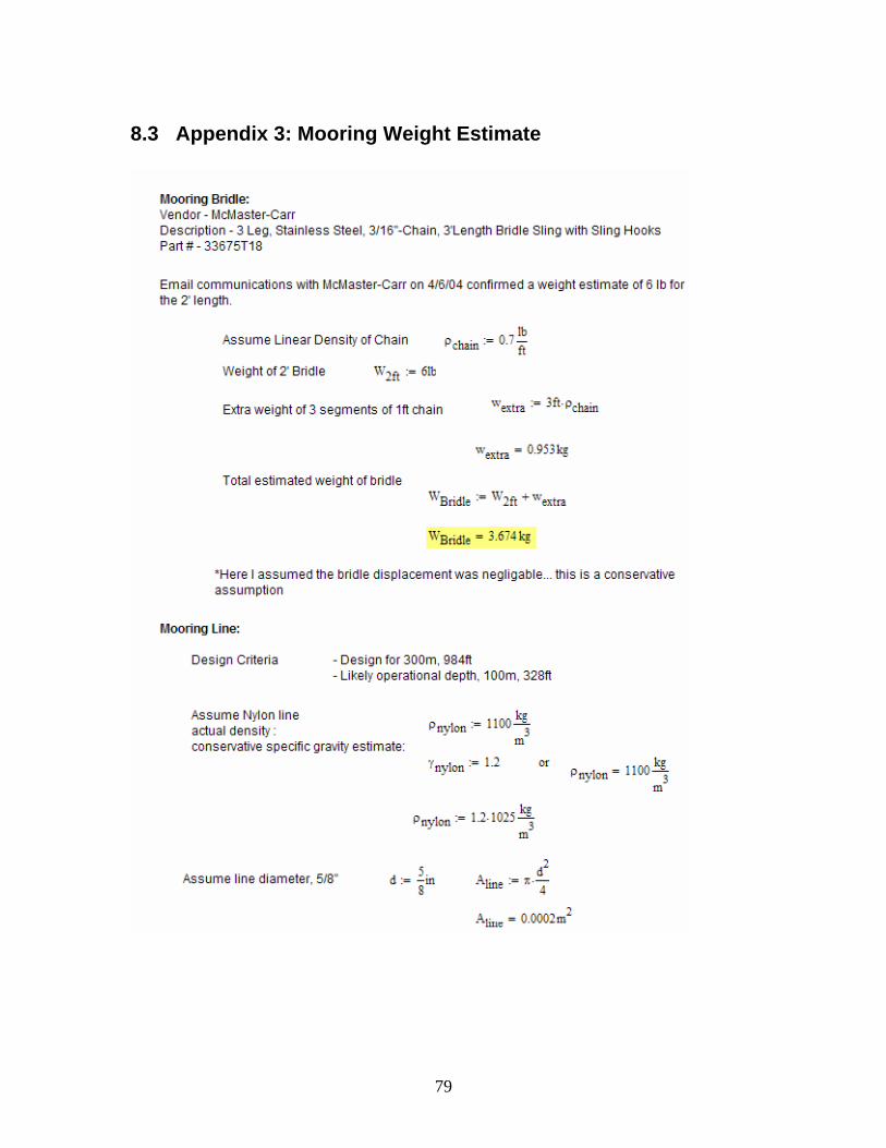
8.3 Appendix 3: Mooring Weight Estimate

79

80