Design of a Low Cost Hydrostatic Bearing

Design of a Low Cost Hydrostatic Bearing

by

Anthony Raymond Wong

Submitted to the Department of Mechanical Engineeringin partial fulfillment of the requirements for the degree ol

Master of Science in Mechanical Engineering

at the

MASSACHUSETTS INSTITUTE OF TECHNOLOGY

MASSACHUSETTS INSTitUTEOF TECHNOLOGY

JUN 2 8 2012

L LIBRARIES

ARCHIVES

June 2012

@ Massachusetts Institute of Technology 2012. All rights reserved.

Author ............... ......... ... . .I . ). . . . . . . . . . . . . . . . . . . . . . . .

Department of Mechan' al EngineeringMay 17, 2012

Certified by. ......... ................... ...... ........ ...Alexander Slocum

Pappalardo Professor of Mechanical EngineeringThesis Supervisor

Accepted by.David E. Hardt

Chairman, Department Committee on Graduate Theses

Design of a Low Cost Hydrostatic Bearing

by

Anthony Raymond Wong

Submitted to the Department of Mechanical Engineeringon May 17, 2012, in partial fulfillment of the

requirements for the degree ofMaster of Science in Mechanical Engineering

Abstract

This thesis presents the design and manufacturing method for a new surface self com-pensating hydrostatic bearing. A lumped resistance model was used to analyze theperformance of the bearing and provide guidance on laying out the bearing features.One arrangement of bearing features was cut into a flat sheet of ultra high molecularweight polyethylene which was then formed into a cylindrical shape. The shapedplastic was adhered to an aluminum housing then connected to a pump. Experi-mental data shows that the lumped resistance model provides a good estimation ofthe bearing performance. After validating the analytical model, sensitivity studieswere conducted to predict changes in the bearing performance due to manufacturingvariances. The results of the model indicate the design is extremely robust.

Thesis Supervisor: Alexander SlocumTitle: Pappalardo Professor of Mechanical Engineering

3

Acknowledgments

I want to start by thanking my God, without whom none of this would be possible.

My father has been an inspiration to me. His stories about MIT made me think

it was somewhere I should go. His constant encouragement made me think MIT was

somwhere I could go. Though he has never studied mechanical engineering, this thesis

is part of his academic legacy.

I don't think words can adequately express my gratitude for my loving wife, Emily.

Thank you for letting me go on this great adventure.

I am also immensely grateful to my thesis advisor, Dr. Alex Slocum. His energy

and creativity motivated me to push forward. He had confidence in me (and the

bearing), when I didn't.

Also I want to thank my lab mates in PERG. Zac Trimble took time from finishing

his thesis to help me get the first test rig built. Folkers Rojas picked up the CFD

and struggled with the theory with me. Mark Belanger at Edgerton Shop and Josh

Dittrich were critical resources in building the hardware.

4

Contents

1 Introduction 13

1.1 M otivation. . . . . . . ... . . . . .. . . . . . . . . . . . . . . . . . 13

1.2 Background . . . . . . . . . . . . . . . . . . . . . . . . . . . . . . . . 14

2 Design 17

2.1 T heory . . . . . . . . . . . . . . . . . . . . . . . . . . . . . . . . . . . 17

2.1.1 Fluid Resistance . . . . . . . . . . . . . . . . . . . . . . . . . 17

2.1.2 Bearing Pad Load. . . . . . . . . . . . . . . . . . . . . . . . . 22

2.1.3 Fluid Resistance Network . . . . . . . . . . . . . . . . . . . . 23

2.1.4 Dimensionless Parameters . . . . . . . . . . . . . . . . . . . . 24

2.1.5 Friction Loss and Temperature Rise . . . . . . . . . . . . . . . 25

2.2 General Design Guidelines . . . . . . . . . . . . . . . . . . . . . . . . 26

2.2.1 Laying Out Hydrostatic Features . . . . . . . . . . . . . . . . 28

2.3 D esign . . . . . . . . . . . . . . . . . . . . . . . . . . . . . . . . . . . 29

3 Results 37

3.1 Half Bearing Proof of Concept . . . . . . . . . . . . . . . . . . . . . . 37

3.2 Half Bearing Design. . . . . . . . . . . . . . . . . . . . . . . . . . . . 38

3.2.1 Sensitivity Study . . . . . . . . . . . . . . . . . . . . . . . . . 42

4 Conclusions 49

4.1 Future Work. . . . . . . . . . . . . . . . . . . . . . . . . . . . . . . . 49

5

A Discretization of the Surface Topology

A. 1 Fluid Resistances

A.1.1

A.1.2

A.1.3

A.1.4

A.1.5

A.2 Load

A.2.1

A.2.2

A.2.3

A.2.4

Compensat

Cross Leak,

Bearing Pa

Leakage .

Supply Lea

Areas . . .

Bearing Pa

Bearing Pa

Inlet ports

Supply Lea

. . . . . . . . . . . . .

or . . . . . . . . . . .

age . . . . . . . . . . .

dg.............

I.............kage . . . . . . . . . .

..Ln...........ds . . . . . . . . . . .

dLands . . . . . . . .

kage . .. . . . . . . .

B Matlab Code

C Technical Drawing

D Calculation of Housing Deflection

6

51

51

52

52

53

54

54

55

56

56

56

56

59

67

71

. . . . . . . . . . . . . . . .

. . . . . . . . . . . . . . . .

List of Figures

2-1

2-2

2-3

2-4

2-5

2-6

2-7

2-8

2-9

2-10

Parallel plate flow . . . . . . . . . . . . . . . . . . . . . . .

Flow through parallel annuli . . . . . . . . . . . . . . . . .

Partial annulus . . . . . . . . . . . . . . . . . . . . . . . .

An eccentric shaft in a bearing . . . . . . . . . . . . . . . .

Rectangular pad with pressure profile . . . . . . . . . . . .

Sketches of the progression of bearing concepts . . . . . . .

Model of pattern cut into flexible material . . . . . . . . .

Resistance network model . . . . . . . . . . . . . . . . . .

Resistance network regions . . . . . . . . . . . . . . . . . .

Resistance network model with the assumed flow direction

3-1 Proof of concept half bearing . . . . . . . . . . . . . . . . . . . .

3-2 Setup for proof of concept half bearing (hoses removed for clarity)

3-3 New housing with UHMW bearing adhered to it . . . . . . . . . .

3-4 New smaller shaft with air bearings to maintain axial position . .

3-5 Final test setup . . . . . . . . . . . . . . . . . . . . . . . . . . . .

3-6 Comparison of calculated and measured load . . . . . . . . . . . .

3-7 Comparison of calculated and measured stiffness . . . . . . . . . .

3-8 Load carrying efficiency . . . . . . . . . . . . . . . . . . . . . . .

3-9 Diagram of collector . . . . . . . . . . . . . . . . . . . . . . . . .

3-10 Load sensitivity to additional collector land angle, psi . . . . . . .

3-11 Flow sensitivity to additional collector land angle, . . . . . . . .

3-12 Bearing performance sensitivity to resistance ratio . . . . . . . . .

7

. . . . . . 17

. . . . . . 19

. . . . . . 20

. . . . . . 21

. . . . . . 22

. . . . . . 30

. . . . . . 30

. . . . . . 31

. . . . . . 32

. . . . . . 33

38

39

40

41

42

43

44

44

45

45

46

46

3-13 Initial specific stiffness times load carrying efficiency plotted against

resistance ratio . . . . . . . . . . . . . . . . . . . . . . . . . . . . . . 47

A-1 Compensator resistance regions . . . . . . . . . . . . . . . . . . . . . 52

A-2 Cross leakage resistance regions (Cross hatched regions are ignored) . 53

A-3 Bearing pad, leakage and supply leakage resistance regions . . . . . . 54

A-4 Load carrying regions . . . . . . . . . . . . . . . . . . . . . . . . . . . 55

D-1 Model of a half of the housing . . . . . . . . . . . . . . . . . . . . . . 71

D-2 The forces and moment on a section of the beam . . . . . . . . . . . 72

8

List of Tables

2.1 Minimum film thickness in im based on shaft surface speed . . . . . 28

3.1 Measurements of 6061 T651 Tube and Half Tubes in mm . . . . . . . 39

9

List of Variables

Symbol Description Units

A, area of lands m2

Ar area of recessed regions m2

c heat capacity k

Db bearing diameter m

e eccentricity

F load carrying efficiency

g acceleration due to gravity 82

h bearing gap m

Hf friction power W

ho gap when shaft is centered m

H, pumping power W

hr recess depth m

k stiffness Nm

k specific stiffness

L length (parallel to fluid flow) m

Lb bearing length m

11

Symbol Description Units

n normal vector

p pressure

NPr recess pressure

PS supply pressure

Q flow rate

Q specific flow rate

R fluid resistanceS

r; inner radius m

r. outer radius m

u fluid velocity in the x direction MS

U relative surface speed m

w width (perpendicular to fluid flow) m

W load N

6 shaft displacement m

AT temperature rise 0C

resistance ratio

0 angle around the bearing 0

p viscosity

p density kg

angle of partial annulus 0

additional collector land angle 0

12

Chapter 1

Introduction

1.1 Motivation

The purpose of this research is to develop a surface self compensating hydrostatic

journal bearing manufactured from a flexible material in a flat state which is then

wrapped into a cylindrical shape and bonded in place. Areas of particular interest

are cost reduction from traditional hydrostatic bearing manufacturing and unique

performance features that can only be leveraged from bearings manufactured by this

method.

The immediate motivation for this research is for naval propeller shafts. One

common way to support propeller shafts are hydrodynamic bearings. Hydrodynamic

bearings have some negative aspects such as wear during slow speeds or changes in the

shaft direction of rotation and ingestion of debris along with the ocean water used to

create the fluid film. A hydrostatic bearing would alleviate these adverse effects, but

generally are more expensive due to complex fluid routing, cost of additional pumps,

susceptibility to fouling or plugging, and multiple precision operations required during

manufacturing. This research seeks to mitigate these impediments.

Another challenge naval bearing design is that sometimes there is a flange on

the end of the shaft. Dry docking to repair bearings can be expensive. In order to

facilitate repair in water without removing the shaft, bearings that are less than a

1800 arc are investigated to fit over the flange. Surface self compensated hydrostatic

13

bearings have usually been made as a full journal bearings and partial arc bearings

have not been made before.

1.2 Background

Hydrostatic bearings appear in the literature as early as 1851 [1]. The basic idea

of a hydrostatic bearing is to pressurize a fluid to produce a fluid film between two

surfaces which move relative to each other. The fluid film thickness is larger than

the surface roughness, so the two surfaces never contact during motion. Additionally,

because of the external fluid pressurization, the supporting force is independent of

surface speed. This insensitivity to relative surface speed differentiates a hydrostatic

bearing from a hydrodynamic bearing. Hydrodynamic journal bearings rely on the

shaft speed to generate the fluid film and forces to support the shaft.

In hydrostatic journal bearings, fluid routings connect load bearing features, or

bearing pads, to a compensator that regulates the fluid flow to the bearing pads

and ensures a pressure differential between opposed load bearing areas, so that the

bearing will apply a force to counteract external loads applied to the shaft. A variety

of compensation methods exist such as fixed compensation which utilizes a fixed fluid

resistance device such as a capillary tube or orifice. Constant flow compensation can

be achieved by using separate pumps for each bearing pad or special valves. This work

is primarily focused on self compensation which uses the gap between the surfaces of

the bearing and the shaft as a variable restrictor to control flow. Early discussion of

self compensation was presented by Hoffer [2]. Self compensation has the advantage

that no tuning is required like fixed compensation. Also self compensation is resistant

to clogging compared to other methods that involve small fluid openings.

Another hydrostatic bearing development of note was invented by Wasson et al.

[3] which involved placement of all fluid routings on the surface of the bearing or shaft.

They called it "surface self compensation" and had the unique feature that since all

the hydraulic logic and connections were on the surface, the motion of the shaft and

fluid shear cleans the surface features and thus it is extremely resistant to clogging. In

14

typical hydrostatic bearings, complex fluid routings move fluid from a compensator

to the opposed bearing pad. These routings increase complexity and increase the

susceptibility of plugging and fouling. Kotilainen and Slocum [4] expanded upon

Wasson's work by casting the surface features into the inner diameter of a bearing

sleeve. Previously, Wasson had machined the features into the outer diameter of the

shaft.

15

Chapter 2

Design

2.1 Theory

2.1.1 Fluid Resistance

-- U(y)h

x

L

Figure 2-1: Parallel plate flow

To understand the theory behind hydrostatic operation, flow between two parallel

plates of width, w, into the page as shown in Figure 2-1 caused by a pressure difference

in the x-direction will be reviewed. The Navier-Stokes equation in the x-direction is

as follows.p (2U

2 U 9 2 u dupg-i of(+2.+1 =Pd (2.1)

Application of (2.1) requires the following conditions:

17

" A newtonian fluid which is true since this discussion is restricted to water

" Constant density which is true as long as temperature does not change signifi-

cantly

" Constant viscosity which is also true as long as temperature does not change

significantly

Assuming that the flow is fully developed, the flow, u, will be a function of y alone.

Additionally, gravity effects will be considered negligible since the x-direction is per-

pendicular to gravity. Applying these assumptions simplifies (2.1) to the following.

op i92U+y =0 (2.2)

&x I'y2 0

Solving (2.2) for the velocity yields the following.

_1 dp y 2

U = d + C1 y + C2 (2.3)y dx 2

No-slip conditions exist at the interface of the fluid and the plates, so u = 0 at y = ih

Solving for the boundary conditions yields the equation for the fluid velocity profile.

1 dp ( 2 h2 (2.4)2p dx 4)

Assuming a constant volume flow rate, the flow rate, Q, can be found by integrating

the velocity profile as follows:

Q = w h' u(y)dyQ /Jh/2-h/2

wha dp12btdp (2.5)12p dx

Solving for the differential pressure yields the following:

dp = -Q 2 dx (2.6)wh3

18

The negative sign in (2.6) indicates that the pressure decreases in the direction of the

flow. At this point, an electrical circuit analogy is useful. Since the relationship in

(2.6) between pressure and flow rate is not time dependent, this system acts like a

resistor. This equation can be formed in a manner similar to Ohm's law, V = IR,

where pressure serves the purpose of voltage and flow rate takes the place of current.

Integrating (2.6) in x from 0 to L yields the following.

p = 2LQ (2.7)wh3

(2.7) assumes that the outlet pressure is zero. From (2.7) it is easy to identify the

resistance term. The fluid resistance of two parallel plates can described as the

coefficients in front of Q. Mathmatically, the resistance is as follows.

Rparae Plates 12 L (2.8)wh 3

d r

Figure 2-2: Flow through parallel annuli

19

Aside from parallel plates, the other geometric configuration that is common in

hydrostatic bearings is two parallel annuli with flow going radially out from the center

as shown in Figure 2-2. Analysis begins with an a thin ring of thickness dr. Because

the thickness of the ring is small compared to the radius, the curvature is ignored and

the parallel rings are modeled as two thin parallel plates of width, 27rr, and length

dr. Substituting these values into (2.6) yields the following.

12piQdrdp = -2 r (2.9)

2-/rks r

Integrating (2.9) from the inner radius of the annulus, ri, to the outer radius, r0,

yields the following equation with the boundary condition of p = 0 at r = r0 :

p = - 1n -Q (2.10)

At the inner radius of the annulus, the pressure is the same as the recess pressure.

Pr - iln - Q (2.11)

Once again, using a circuit analogy gives the following equation for the fluid resistance.

RAnnulus = 6 n (o (2.12)

For partial annular lands which are not a full circle as in Figure 2-3, (2.12) can be

Figure 2-3: Partial annulus

20

modified to the following.

RAnnulus= 6p n ro 36007rha (ri 4

(2.13)

where # is the angle that the circular land covers in degrees.

Figure 2-4: An eccentric shaft in a bearing

While these analyses for parallel surfaces are convenient from an analysis stand-

point, in most cases of interest surfaces in a journal bearing are not parallel. If the

shaft is not centered as shown in Figure 2-4, the gap is not constant. For a shaft that

is not centered, the shaft eccentricity is defined as

e = -- (2.14)ho

In (2.14) h, is the bearing gap at a reference position. For journal bearings, the

reference position is when the shaft and bearing are concentric. 6 is the distance

between the axes of the shaft and bearing. The bearing gap, h, can then be described

as a function of eccentricity and angle, where the angle is measured from the line

21

going through the centerlines of the bearing and shaft.

h = h0 [1 - e cos(O)] (2.15)

(2.15) could then be substituted into (2.6). However, Kotilainen [5] numerically shows

that for hydrostatic journal bearing design approximating these surfaces as parallel

plates is sufficient for calculating resistances and is accurate to within 4% when the

feature circumferential width is less than 10% of the diameter.

2.1.2 Bearing Pad Load

PrAAA

E/ [ /E

Lieft Lrecess Lright

Figure 2-5: Rectangular pad with pressure profile

Hydrostatic bearings are usually comprised of load carrying areas called bearing

pads. Bearing pads are recesses surrounded by raised lands. The pressure in the recess

is considered constant due to its depth. This assumption arises from (2.6). When

h is large, dp becomes small especially since the relationship is cubic. In the lands,

the pressure decreases to the pressure outside the bearing pad, usually atmospheric

pressure. The load from any fluid can be calculated by integrating the pressure:

W = pndA (2.16)

where n is the normal vector. For the example in a long rectangular bearing pad as in

22

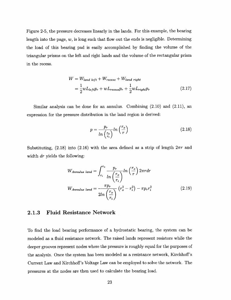
Figure 2-5, the pressure decreases linearly in the lands. For this example, the bearing

length into the page, w, is long such that flow out the ends is negligible. Determining

the load of this bearing pad is easily accomplished by finding the volume of the

triangular prisms on the left and right lands and the volume of the rectangular prism

in the recess.

W = Wiand left + Wrecess + Wiand right1 1= wLieftPr + wLrecessPr + 1wLrightPr (2.17)22

Similar analysis can be done for an annulus. Combining (2.10) and (2.11), an

expression for the pressure distribution in the land region is derived:

p = 1 n ( ) (2.18)in ( r ,

Substituting, (2.18) into (2.16) with the area defined as a strip of length 2frr and

width dr yields the following:

WAnnulus land = j Pr in () 2,rrdrfir n -o -

(r )

WAnnulus land = 2inQ2) (r2 - r) - fPr ri (2.19)

(r)

2.1.3 Fluid Resistance Network

To find the load bearing performance of a hydrostatic bearing, the system can be

modeled as a fluid resistance network. The raised lands represent resistors while the

deeper grooves represent nodes where the pressure is roughly equal for the purposes of

the analysis. Once the system has been modeled as a resistance network, Kirchhoff's

Current Law and Kirchhoff's Voltage Law can be employed to solve the network. The

pressures at the nodes are then used to calculate the bearing load.

23

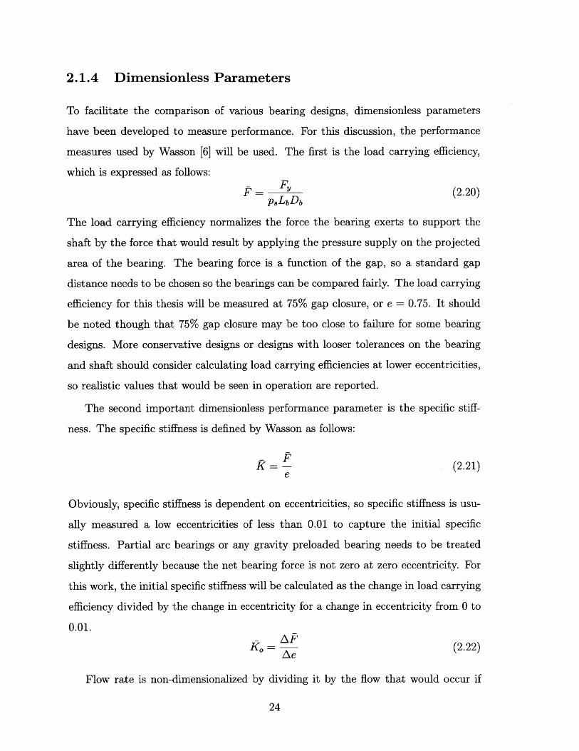
2.1.4 Dimensionless Parameters

To facilitate the comparison of various bearing designs, dimensionless parameters

have been developed to measure performance. For this discussion, the performance

measures used by Wasson [6] will be used. The first is the load carrying efficiency,

which is expressed as follows:

F = (2.20)pLbDb

The load carrying efficiency normalizes the force the bearing exerts to support the

shaft by the force that would result by applying the pressure supply on the projected

area of the bearing. The bearing force is a function of the gap, so a standard gap

distance needs to be chosen so the bearings can be compared fairly. The load carrying

efficiency for this thesis will be measured at 75% gap closure, or e = 0.75. It should

be noted though that 75% gap closure may be too close to failure for some bearing

designs. More conservative designs or designs with looser tolerances on the bearing

and shaft should consider calculating load carrying efficiencies at lower eccentricities,

so realistic values that would be seen in operation are reported.

The second important dimensionless performance parameter is the specific stiff-

ness. The specific stiffness is defined by Wasson as follows:

K = - (2.21)e

Obviously, specific stiffness is dependent on eccentricities, so specific stiffness is usu-

ally measured a low eccentricities of less than 0.01 to capture the initial specific

stiffness. Partial arc bearings or any gravity preloaded bearing needs to be treated

slightly differently because the net bearing force is not zero at zero eccentricity. For

this work, the initial specific stiffness will be calculated as the change in load carrying

efficiency divided by the change in eccentricity for a change in eccentricity from 0 to

0.01.

Ko - A (2.22)de

Flow rate is non-dimensionalized by dividing it by the flow that would occur if

24

the flow went through an annulus the same size as the clearance when the shaft is

centered in the bearing. The formula for specific flow rate is as follows:

Q = D (2.23)p,7sDbho

12pLb

Resistance ratio is another variable frequently used in the design of bearings. It is

the ratio of the inlet fluid resistance across the compensator to the outlet resistance

across the lands.

(= " (2.24)Rout

2.1.5 Friction Loss and Temperature Rise

Because of friction losses due to shearing the fluid, hydrostatic bearings will cause

a rise in temperature of the fluid. The friction power is the power needed to shear

the fluid when two surfaces move relative to each other. It can be calculated by the

following from [7].

Hf = pU 2 (, + (2.25)(h hr

Here U is the relative surface speed and for a journal bearing is a function of the

angular velocity of the shaft. The two terms in (2.25) represent the power loss due to

friction for the lands and recesses, respectively. The coefficient of four for the recess

friction term is a correction for recirculation flow in the recess. The pumping power,

or power needed to move the fluid through the bearing, is defined as the following:

2

H, = pQ = (2.26)

These two power losses become the total power dissipated by the bearing, or

Ht = Hp + Hf (2.27)

25

Both terms in (2.27) are related the bearing gap and can be written as follows.

Ht = C1h3 + C2 (2.28)h

C1 is a related to the land geometry and supply pressure. C2 is related to the surface

area of the bearing and surface speed of the shaft. It can immediately be seen that

pumping losses increase with bearing gap while shear losses decrease with increasing

gap.

The temperature rise can then be described as follows.

AT = HQcp

- +sH1+(2.29)

When the shaft is not rotating, the temperature rise in the fluid simplifies to the

following.

AT Ps (2.30)cp

For water, which is the fluid of interest, at 200C, the temperature rise (0C) due to

supply pressure only is

AT = 2.397X10- 7ps (2.31)

where p, is the pump supply pressure in N/m2

2.2 General Design Guidelines

Given the previous discussion concerning the theory behind hydrostatic bearings, the

design of such a bearing may appear intimidating. However, design of a hydrostatic

bearing is actually fairly straight forward. Suppose a problem begins with a shaft of

a certain diameter and load that needs to be supported.

1. Size a pump to see if it is feasible to support the load with a given pumping

pressure. As a general rule of thumb the load carrying efficiency of a surface

26

self compensated bearing is 0.2-0.3. Using equation (2.20) the load that the

bearing could support can be calculated.

2. The bearing gap should be determined. The performance with respect to pump-

ing power is improved by reducing the bearing gap, while shear power is worse

with decreasing gap. In later stages of design after the bearing features have

been determined, the bearing should be optimized to reduce power losses by

finding the minimum power from (2.28). To start though, DIN standard 31652

[8] provides the information in Table 2.1 for minimum film thickness for hy-

drodynamic bearings. These empirical recommendations assume peak to valley

surface roughness of less than 4 Rm, minor geometrical errors, filtering of the

fluid and running-in of the bearing. This table gives the lower bound of the

bearing gap to prevent contact between the asperities on the shaft and bear-

ing. Manufacturing limitations will prevent most designs from using such small

bearing gaps. Another rule of thumb in hydrodynamic bearing design is to use

a bearing radius to radial bearing gap ratio of 1000 [9]. For lack of better guide-

lines this rule of thumb will suffice as a starting point for hydrstatic bearing

designs. Finally, one other consideration for bearing gap is the ratio of gap to

groove depth. Usually the bearing gap will drive the groove depth and not the

other way around, but for bearings cut into flat sheets the limits on the sheet

thickness may cause issues. For the grooves to function as nodes they need

to be significantly lower resistance than the raised lands. At a minimum the

grooves should be 10 times deeper than the bearing gap. Ideally, they should

be 15 times the bearing gap.

3. Determine the bearing length to diameter ratio based on the space available.

The length should be at least as large as the diameter for pure radial support.

If moment loads need to be supported, two bearings each of at least one shaft

diameter in length should be about 3 shaft diameters apart center to center.

This rule of thumb comes from Saint-Venant's principle.

4. Select the circumerferential angle the bearing will cover. Partial arc bearings

27

Table 2.1: Minimum film thickness in Rm based on shaft surface speed

Shaft diameter Sliding speed of shaft

(mm) (m/s)Over - 1 3 10 30

_ Upto 1 3 10 30 -24 63 3 4 5 7 1063 160 4 5 7 9 12

160 400 6 7 9 11 14400 1000 8 9 11 13 161000 2500 10 12 14 16 18

much less than 1800 will have problems creating opposed differential pressure

to recenter the shaft from perturbations. Also partial arc bearings have circum-

ferential leak paths, so they will require more flow than a full journal bearing

where fluid can only exit axially. Knowing the length, diameter and angle of

coverage, a rectangular footprint available for the hydrostatic features can be

determined.

2.2.1 Laying Out Hydrostatic Features

Now that the available area for the hydrostatic features is bounded, grooves need to

be designed to route the fluid and make the surface self compensating bearing. There

is great latitude in what could work. The following discussion attempts to provide

some suggestions on how to start.

1. Start by placing the inlets. The radial position of the shaft will be sensed in the

region around the inlets. The inlets should be distributed in such a way that

the bearing is sensitive to shaft movement in directions needed for the design.

2. Separate the inlet port from a collector groove with a land region. This land

will be the compensating resistor and control the flow to the bearing pad.

3. Place the load carrying areas nominally on the opposite side of the shaft. The

positions of the load carrying areas and compensators are crucial, since the

28

compensator will sense the location of the shaft and the load carrying areas will

apply the reaction force.

4. Connect the collector to the load carrying area with a groove.

5. Model the surface as a node network. Treat the recessed areas as nodes. Account

for all the flow going out of the inlets and in and out of the nodes.

6. Divide the surface into logical sub regions for calculations. From the discussion

in 2.1.1, keep the circumferential width of the sub regions less than 10% of the

diameter, so a single gap value can be used for the sub region. Using circular and

rectangular sub regions eases calculations. Divide up the lands into regions to

calculate the resistances. Divide the load bearing pads into regions to calculate

the forces.

7. Based on the dimensions of the region calculate fluid resistances between re-

gions. Use the distances from the assumed direction of shaft movement to

calculate the angle of the land. Calculate the bearing gaps by using (2.15).

8. Solve the node network for the pressures in the recesses.

9. Calculate forces from the bearing pads.

10. Adjust the geometry to achieve the desired performance.

See Appendix A for an example of how the surface of a bearing was discretized

into lumped resistances and analyzed to determine performance.

2.3 Design

The initial concept for the partial arc bearing included two pockets as shown in Figure

2-6a. In these concept sketches the circular areas represent the inlet and compensator.

The rectangles represent the bearing pad areas. In the first concept, the center of

the bearing pads are offset axially and would allow a twisting moment on the shaft.

Figure 2-6b shows a second concept that removes the twisting moment at the expense

29

a b C

Figure 2-6: Sketches of the progression of bearing concepts

Figure 2-7: Model of pattern cut into flexible material

of bearing pad area. If the bearing pads are thought of as point loads, the shaft is

supported by only two points. No matter how arranged, two support points are not

stable and a second bearing would be required. In the final concept a third pocket

was added to provide tilt stiffness and resist twist shown in Figure 2-6c. The bearing

features were designed to be machined into a flat flexible material and adhered to

half of a cylinder. The pattern for the test bearing is shown in the left side of Figure

2-7. The cross-hatched circular regions are the inlets. The hatched regions are the

recessed areas while the white areas are the raised lands. A rendering of the bearing

formed into a cylinder is shown on the right side of Figure 2-7. Sensitivity studies

30

M

examining the amount of collector wrap and collector land thickness are discussed

in section 3.2.1. The bearing covers 1650 of the the shaft and was designed for a

nominal bearing gap of 127 Rm for a shaft diameter of 100 mm. The groove depth

was selected to be 10 times deeper than the bearing gap. Since the resistance is

inversely proportional to the gap cubed, the resistance in the grooves would be 1000

times less than the raised areas. This low resistance allows the grooves to be treated

as constant pressure nodes.

Rc1 Rc2 Rc3

1 2' 2 \ 3 SRCL1 RCL2

R, 1 RL1 RP2 RP3 RL3

Figure 2-8: Resistance network model

Based on the previously discussed theory, the bearing surface is modeled as a

resistance node network shown in Figure 2-8. The subscript 'C' indicates that the

resistance is for the compensator, 'CL' for cross leakage between nodes, 'P' for leakage

out of the load bearing pad, 'L' for leakage, and 'SL' for supply leakage directly from

the inlet to the bearing outlet. Figure 2-9 shows how the topology of the bearing was

turned into resistances. The hatched regions are numbered and indicate the nodes or

constant pressure regions. Further discussion of how the topology was lumped into

31

Figure 2-9: Resistance network regions

resistances is discussed in Appendix A.

For the resistance calculation, the geometry of the region is needed as well as the

fluid viscosity and density. For these calculations, the viscosity and density of water

at 20*C were used, 1.003x 10- 3 Ns/m 2 and 998 kg/m 3 , respectively. For rectangular

regions, (2.8) was used. The length and width of the rectangular lands were taken

from the technical drawing in Appendix C. Calculations were only done for the shaft

moving down toward the center of the flexible sheet, so the distance to the center of

the land from the center of the flexible bearing material was used to calculate the

arc length and combined with the nominal diameter of the bearing could be used

to calculate the angle, 0, as shown in Figure 2-4. (2.15) was then used to calculate

32

the bearing gap for the land. For circular lands, a similar approach was used. The

distance from the center of the circle was used to calculate the angle of the feature

in the formed state. Then the angle was used to calculate the bearing gap at that

location. The inner and outer radii from the drawing were used to calculate the

resistance.

IQSL

Reqi

Req = R,RL1* Rpl+RL

R3 = RP3RL3eq3 RP3+RL3

Figure 2-10: Resistance network model with the assumed flow direction

Using basic circuit theory, the pressures and flow rates can be solved for in a

straight forward manner. Figure 2-10 shows the resistance network again but with

assumed flow directions. The supply leakage flow is ignored for now because it can be

solved for directly using the equation P = QR. Reqi and Req3 represent the equivalent

resistance of the bearing pad lands and the leakage lands for bearing pads 1 and 3.

Eight equations are needed to solve the network for the eight unknowns, Qci, Qc2,

QC3, QcL1, QcL2, Qeq1, QP2, and Qeq3. First Kirchhoff's Current Law can be applied

to each node, which is equivalent to conservation of mass - the combined flows in and

33

out of each node must equal zero.

Qci - QcL1 - Qeqi = 0

Qc2 + QcL1 - QCL2 - QP2 = 0

QC3 + QcL2 - Qeq3 = 0 (2-32)

Next Kirchhoff's Voltage Law provides two more equations. These equations state

that the net pressure change going around the upper loops is zero.

Rc1Qc1 + RcL1QCL1 - Rc2Qc2 = 0

Rc2Qc2 + RCL2QCL2 - Rc3Qc3 = 0 (2.33)

Finally, three more equations are provided by realizing that the pressure drop across

the compensator and the outlet must equal the supply pressure.

Rc1Qc1 + Req1Qeq1 = Ps

Rc2Qc2 + RP2QP2 Ps

Rc3Qc 3 + Req3Qeq3 = P, (2.34)

Equations (2.32), (2.33) and (2.34) form the following matrix equation which is easily

solved by Matlab.

1 0 0 -1 0 -1 0 0

0 1 0 1 -1 0 -1 0

0 0 1 0 1 0 0 -1

Rci -Rc 2 0 RcL1 0 0 0 0

0 Rc 2 -RC 3 0 RCL2 0 0 0

Rc1 0 0 0 0 Reqi

0 RC 2

0 0

0 0

0 0

0 0 RP 2 0

Rc 3 0 0 0 0 Req3

Qc1

Qc2

Qc3

QCL1

QCL2

Qeqi

QP2

Qeq3

0

0

0

0

0

PS

PS

PS

(2.35)

34

As mentioned earlier the supply leakage flow can be calculated using the circuit anal-

ogy mentioned in 2.1.1 such that P = QR. During design iterations it is worthwhile

to examine the proportion of leakage flow to total flow. The proportion of leakage

flow to total flow will vary based on the number of inlets, bearing arc, and load car-

rying efficiency. Large lands can be placed next to the inlets and grooves that route

fluid to reduce leakage, but those lands will not improve the loads the bearing can

support and will lower load carrying efficiency. Determining an appropriate amount

of leakage flow is a trade off and requires engineering judgement.

The pressures of the nodes are found by multiplying the flow rates by the resis-

tances. The three node pressures are calculated with the following equations.

P1 = Req1Qeq1

P 2 = RP 2 QP 2

P3 = Req3Qeq3 (2.36)

With these pressures, (2.17) is then be used to calculated the bearing pad forces.

(2.19) along with the inlet pressure calculates the forces in the supply leakage region.

The force at the inlet port is calculated by multiplying the inlet pressure by the inlet

area. At this point the forces and flow rates have been solved for and dimensionless

parameters are calculated to characterize the bearing.

Using this basic methodology, dimensions from CAD were input into a Matlab

script and then the performance of the bearing was analyzed. Appendix B includes

example code used to analyze this bearing.

35

Chapter 3

Results

3.1 Half Bearing Proof of Concept

For the halfbearing, features were machined into 2.54 mm thick adhesive-backed ultra

high molecular weight (UHMW) polyethylene. In the proof of concept, the bearing

was bonded into a 6061 T651 aluminum half cylinder. The half cylinder was turned

in a lathe then cut in half. The design was sized to fit a precision ground 100 mm

diameter shaft from another project. Initially, the bearing would not work and it

was thought that the tube had collapsed when it was cut. The half cylinder was put

in a hydraulic press to plastically deform the aluminum slightly which then allowed

the shaft to float freely. Due to lack of measurement equipment, the amount of

deformation was not quantified. The first half-bearing prototype is shown in Figure

3-1. In the picture the large diameter disc behind the shaft is an automotive brake

rotor which was used as an axial rolling bearing to take up thrust loads. This initial

prototype showed that the bearing design could support a shaft with a fluid film.

Samples of 6061 T651 aluminum tube with a nominal ID of 101.6 mm and OD

of 127 mm were sent to NIST and measured on a Cordax CMM. Table 3.1 shows

the diameter and cylindricity of the tube and the two halves after it was cut in half

axially. As can be seen from the data, the tube opened up slightly after being cut.

The change in diameter is significant compared to the designed bearing gap of 127

Rm, which lends credence to the theory that though the inner diameter was machined

37

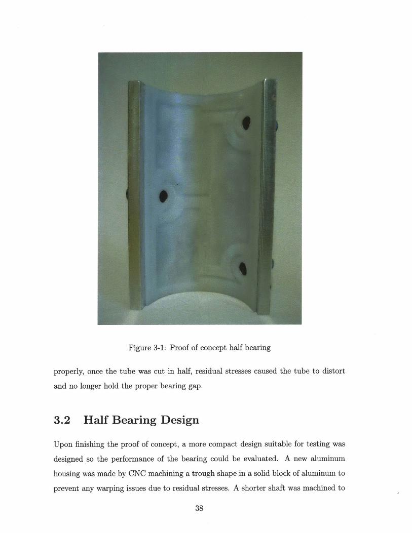
Figure 3-1: Proof of concept half bearing

properly, once the tube was cut in half, residual stresses caused the tube to distort

and no longer hold the proper bearing gap.

3.2 Half Bearing Design

Upon finishing the proof of concept, a more compact design suitable for testing was

designed so the performance of the bearing could be evaluated. A new aluminum

housing was made by CNC machining a trough shape in a solid block of aluminum to

prevent any warping issues due to residual stresses. A shorter shaft was machined to

38

Figure 3-2: Setup for proof of concept half bearing (hoses removed for clarity)

Table 3.1: Measurements of 6061 T651 Tube and Half Tubes in mm

Inner Surface Outer SurfaceS Cyl 0 Cyl

Tube 101.521 0.211 126.818 0.242Half 1 101.638 0.075 126.915 0.101Half 2 101.653 0.054 127.015 0.079

provide a 12 7km nominal gap. To address concerns about the UHMW delaminating

from the aluminum, the aluminum housing, plastic and shaft were heated to 130*C

in an oven with a 127pm sheet of shim stock between the shaft and the plastic to

thermally form the plastic to the proper gap where the gap would ideally be the

thickness of the shim stock. This process reduced the stresses in the plastic and

helped the plastic to bond better to the aluminum. Figure 3-3 shows the plastic

bonded into the aluminum housing after thermoforming. Figure 3-4 shows the new

shaft. A new test setup was built for the bearing which includes a dedicated impeller

pump, filter, flow meter, digital pressure readout, and ball valves for flow control in the

fluid circuit. Air bearings are used to constrain the shaft axially. A compressed gas

39

Figure 3-3: New housing with UHMW bearing adhered to it

cylinder was included to supply the air bearings to eliminate any noise that might have

been introduced by a compressor. An Admet 5604 single column universal testing

machine and an Interface 1210ACK-300-B load cell rated for 300 lbs are used for

applying load to the shaft. The 5604 is driven by Admet's MTestQuattro software.

Lion Precision U3B eddy current probes driven by ECL202 drivers measure the shaft

location. All these components were installed on a stand alone cart fabricated from

T-slot structural framing. The cart is on wheels to allow the test apparatus to be

easily moved after the water reservoir has been filled. The MTestQuattro system

records readings from the load cell, eddy current probes, and pressure gauge. Figure

3-5 shows the cart with the attached equipment.

Figure 3-6 shows the calculated and measured vertical load that the bearing sup-

ports. The calculated values come from the Matlab script in Appendix B solving the

hydraulic resistance network model for the bearing. Figure 3-7 shows the stiffness of

the bearing, or the slope of the previous curve, where the stiffness is defined as the

change in force divided by the change in bearing gap, k = AF/Ah. These two graphs

demonstrate the hydraulic resistance model reasonably predicts the performance of

the bearing and hence the design is deterministic. Figure 3-8 shows the measured

40

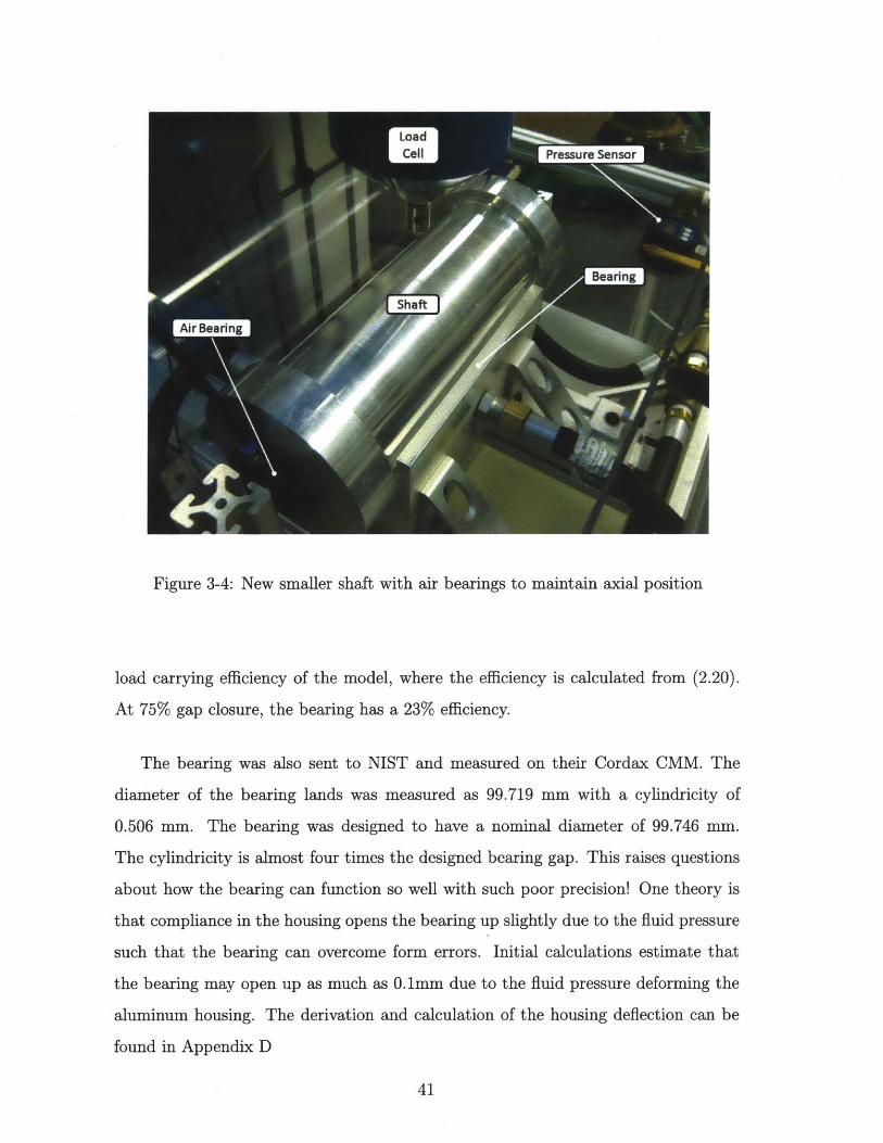
Figure 3-4: New smaller shaft with air bearings to maintain axial position

load carrying efficiency of the model, where the efficiency is calculated from (2.20).

At 75% gap closure, the bearing has a 23% efficiency.

The bearing was also sent to NIST and measured on their Cordax CMM. The

diameter of the bearing lands was measured as 99.719 mm with a cylindricity of

0.506 mm. The bearing was designed to have a nominal diameter of 99.746 mm.

The cylindricity is almost four times the designed bearing gap. This raises questions

about how the bearing can function so well with such poor precision! One theory is

that compliance in the housing opens the bearing up slightly due to the fluid pressure

such that the bearing can overcome form errors. Initial calculations estimate that

the bearing may open up as much as 0.1mm due to the fluid pressure deforming the

aluminum housing. The derivation and calculation of the housing deflection can be

found in Appendix D

41

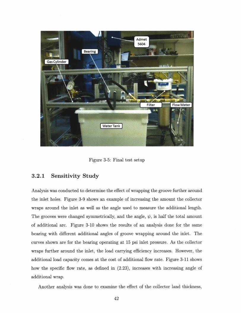
Figure 3-5: Final test setup

3.2.1 Sensitivity Study

Analysis was conducted to determine the effect of wrapping the groove further around

the inlet holes. Figure 3-9 shows an example of increasing the amount the collector

wraps around the inlet as well as the angle used to measure the additional length.

The grooves were changed symmetrically, and the angle, @b, is half the total amount

of additional arc. Figure 3-10 shows the results of an analysis done for the same

bearing with different additional angles of groove wrapping around the inlet. The

curves shown are for the bearing operating at 15 psi inlet pressure. As the collector

wraps further around the inlet, the load carrying efficiency increases. However, the

additional load capacity comes at the cost of additional flow rate. Figure 3-11 shows

how the specific flow rate, as defined in (2.23), increases with increasing angle of

additional wrap.

Another analysis was done to examine the effect of the collector land thickness,

42

800

' 600

0 '"-J-- 400-

200-

- -'Calculated- Measured

-8.2 0 0.2 0.4 0.6 0.8Eccentricity

Figure 3-6: Comparison of calculated and measured load

T, shown in Figure 3-9. This land can be adjusted to change the fluid resistance of

the compensator and thus the resistance ratio, which is defined as the ratio of the

resistance of the inlet to the resistance of the outlet. Figure 3-12 shows the results.

The abscissa is the resistance ratio at zero eccentricity averaged over the three pockets.

The initial specific stiffness is calculated as a change in load carrying efficiency for

a change in eccentricity from 0 to 0.01 divided by the change in eccentricity. The

reported load carrying efficiency is calculated at 75% gap closure. As can be seen,

varying the resistance ratio trades load carrying efficiency for stiffness, and both

cannot be optimized simultaneously by means of the resistance ratio alone. Figure

3-13 shows the product of the two curves in Figure 3-12 plotted against the resistance

ratio. The maximum occurs at a resistance ratio of 0.4651.

43

5 x 1,- Calculated

4.5 - - Measured

0 0.2 0.4Eccentricity

Figure 3-7: Comparison of calculated and measured stiffness

0 0.2 0.4 0.6Eccentricity

Figure 3-8: Load carrying efficiency

44

4[

3.5 F

i

z

U)

2.5[

1.5-. I 0.6 0.8

0.24 . .-- MeasuredI

0.23-

0.22-

0.21 -0ci 0.2F

0.19 -

0.18-

0.8

3

LIJ

T

Figure 3-9: Diagram of collector

0.3-

0.28-

-D 0.26-

S0.24 -

0.220CO0 i

0.2

0.18 -0 0.2 0.4 0.6

Eccentricity0.8

Figure 3-10: Load sensitivity to additional collector land angle, psi

45

0.80.2 0.4 0.6Eccentricity

Figure 3-11: Flow sensitivity to additional collector land angle, 0p

0'0 0.5 1 1.5

Average Resistance Ratio

0.6

w

Ca

0

-j

0.2

Figure 3-12: Bearing performance sensitivity to resistance ratio

46

20

a)

0

(0

.

II

15

10

5

O-0

0.04

(1 0.03

: 0.02

a 0.01C,)

0.015

0.014-

0.013-

0.012-

0.011 -

0.01 -

0.009-

0.008-

0.007-

0.006-

0.0050 0.2 0.4 0.6 0.8 1 1.2 1.4 1.6

Average Resistance Ratio

Figure 3-13: Initial specific stiffness times load carrying efficiency plotted againstresistance ratio

47

Chapter 4

Conclusions

This work demonstrates the deterministic design theory for a surface self compen-

sated hydrostatic bearing covering less than 1800 of the shaft surface. This paper

evaluates just one half of a bearing to support a horizontal heavy shaft and analyzes

the sensitivities of the bearing performance to the some of the design parameters. In

practice though the bearings could be paired to provide preload on the other side of

the shaft. Also a method to manufacture such a bearing is presented. This bearing

design, being a partial arc, facilitates installation and repair of hydrostatic bearings

in support of large shafts since it does not need to be slid over the end of the shaft.

4.1 Future Work

Future work will investigate the hydrodynamic performance of this type of bearing.

The ultimate goal is to be able to produce a low cost bearing which runs hydrostaticly

at low shaft speeds and hydrodynamically at high shaft speeds to reduce operating

cost by allowing pumping power to be reduced.

Other manufacturing methods should also be pursued to reduce the cost and

time to make these bearings. Specifically, examining methods that would allow an

as-extruded tube, casting, or forging to be used as the bearing housing would be

significantly cheaper than using a CNC machined trough. Table 3.1 shows that the

cylindricity of the as-extruded aluminum half tube is two orders of magnitude lower

49

than the UHMW thickness. UHMW may be able to be thermoformed to fill in the

errors in the tube while also replicating a master shaft diameter.

Other topologies should also be investigated. The pattern of grooves presented in

this thesis is by no means the only pattern. Other topologies potentially have better

performance or could be optimized for different applications.

Finally, the bearing has been shown to be very robust. Further investigation is

needed to understand how the bearing can still function with so much form error.

50

Appendix A

Discretization of the Surface

Topology

A.1 Fluid Resistances

The surface of the bearing needs to be divided up into regions and a resistance

value needs to be determined for the regions. The size of the regions requires some

balancing. On the one hand, if the regions are too large, the results may become

unreliable especially if a single gap measurement is used for a large area. On the

other hand, as the regions get smaller, computational time is increased. One could

imagine that if very fine regions are used, the problem turns into CFD. The power in

the lumped resistance network lies in the ease of setting up the problem and speed

of computation without sacrificing accuracy significantly. As part of the effort to

balance fidelity with ease, some regions are double counted and some are not counted

at all to make setting up the problem easier. The following subsections will show how

the surface was divided up into regions and turned into fluid resistances.

Concerning nomenclature, the subscript 'C' indicates that the resistance is for the

compensator, 'CL' for cross leakage between nodes, 'P' for leakage out of the load

bearing pad, 'L' for leakage, and 'SL' for supply leakage directly from the inlet to

the bearing outlet. The first numerical subscript indicates which node the region is

related to. The second numerical subscript after the underscore indicates a subregion

51

within that category of regions. The resistor icons indicates the assumed direction of

flow. Tilting of the shaft was ignored, so all gap measurements come from (2.15).

A.1.1 Compensator

Figure A-1: Compensator resistance regions

Figure A-1 shows the regions used for the compensator resistance for inlet 1 on

the right and inlet 2 on the left. Inlet 3 is the mirror image of inlet 1. This region is

treated as a flow going radially outward from half an annululus per (2.13). The gap

at the center of the inlet was used as the gap for this region.

A.1.2 Cross Leakage

Figure A-2 shows the regions used for the leakage between the recessed regions shown

with the hatching. The cross-hatched regions indicate areas that were ignored. The

fluid flow is parallel to the resistor icons. The bolded lines indicate the edges of

the regions being discussed. The dot-filled regions indicate areas that were double

counted. RCLi-1, RcL1, Rci_3, RCL2_1, RCL22, and RCL2_a are all treated as rect-

angular parallel plates according to (2.8). The gap at the center of the region was

used in calculating the resistances. RcLi_4 and RcL2_4 are treated as a quarter of an

annular region flowing radially outward. These regions slightly overlap with RcL1_3

and RCL2_3 as shown by the dotted areas. The gap at the center of P_1 and P3 _1

shown in Figure A-4 were used for calculating the resistances of these regions. RcL1_5

52

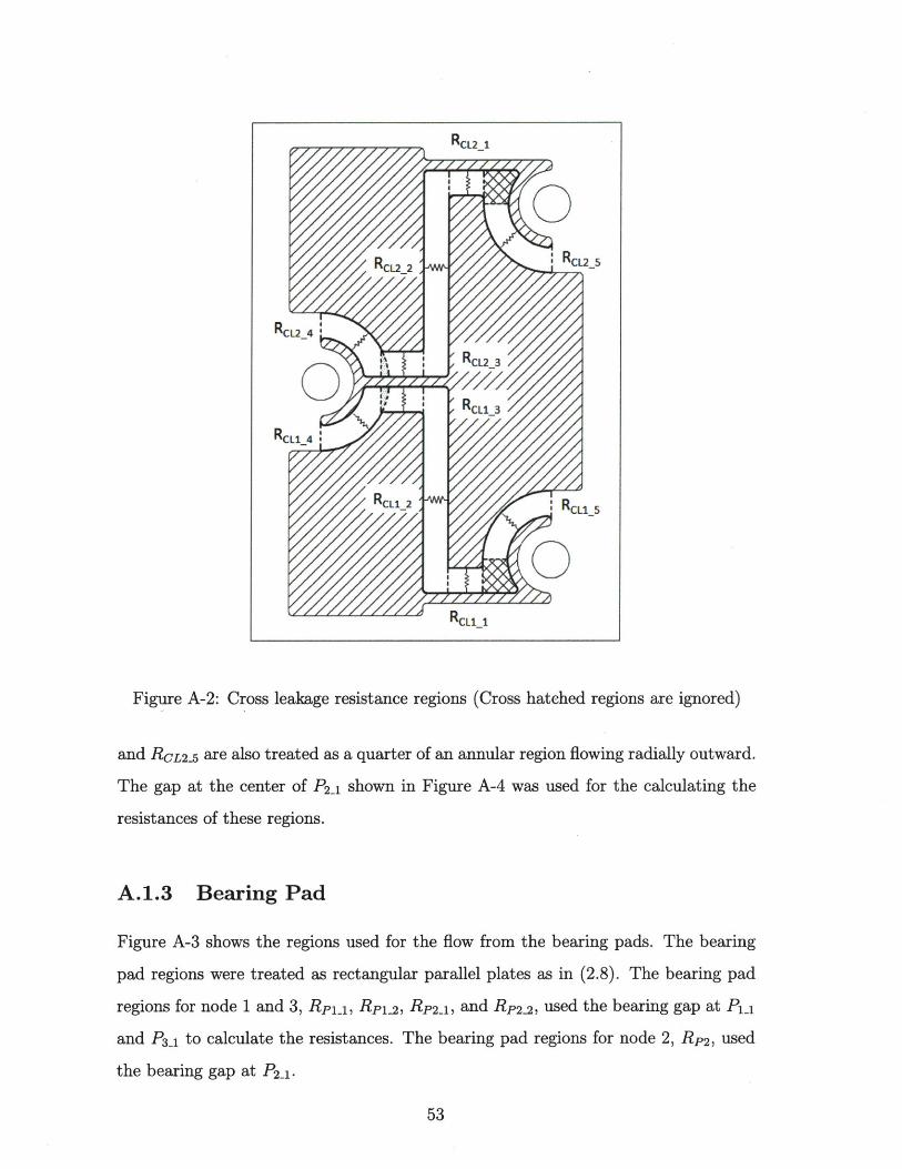
Figure A-2: Cross leakage resistance regions (Cross hatched regions are ignored)

and RCL2- are also treated as a quarter of an annular region flowing radially outward.

The gap at the center of P2 _1 shown in Figure A-4 was used for the calculating the

resistances of these regions.

A.1.3 Bearing Pad

Figure A-3 shows the regions used for the flow from the bearing pads. The bearing

pad regions were treated as rectangular parallel plates as in (2.8). The bearing pad

regions for node 1 and 3, Rpu-, Rpu-, RP2_i, and RP2_2 , used the bearing gap at P1_1

and P3_1 to calculate the resistances. The bearing pad regions for node 2, RP2 , used

the bearing gap at P2 _1.

53

Figure A-3: Bearing pad, leakage and supply leakage resistance regions

A.1.4 Leakage

Leakage regions were defined as in Figure A-3. These regions account for leakage

from the grooves connecting the collectors to their respective bearing pads and were

separated from the bearing pad regions to be able to track flows that did not con-

tribute to bearing performance. For these leakage regions the gap at the center of the

inlet was used for computing the resistance.

A.1.5 Supply Leakage

The leakage directly from the inlets to atmospheric pressure were tracked to be able

to calculate total flow rate needed from the pump. The regions were treated as half

54

annular regions per (2.13). The gap at the center of the inlet was used for these

resistances.

A.2 Load Areas

Figure A-4: Load carrying regions

For calculating the force from the bearing, the load carrying areas were broken

up into regions and the load was calculated similar to (2.17). The recessed bearing

pad regions are denoted by 'P' with the subscript numerals similar to the resistance

nomenclature. The bearing pad lands, or lands next to the bearing pads, are marked

'PL'. The inlet ports are marked 'I'. The assumed region for supply leakage are labeled

55

W

'SL'. Angles were assumed and used to calculate the force component in the vertical

direction for each region.

A.2.1 Bearing Pads

The recessed bearing pads were each divided into two regions shows in Figure A-4.

The cross-hatched areas in Figure A-4 were not considered in the calculation of forces.

The force was considered to be applied from the center of the regions for calculating

the angle the force acted in. The forces in the bearing pads were calculated by

multiplying the recess pressure by the area.

A.2.2 Bearing Pad Lands

The bearing pad lands for node 1 and 3 were divided into three parts as can be seen

in Figure A-4. The pressure in these pad lands were considered to be decreasing

linearly from the bearing pad recess pressure, so the pad land forces were calculated

as half the recess pressure multiplied by the area similar to (2.17). The forces from

PL 1 1 , PL 1 2 , PL 3.1, and PL 3 2 were treated as acting at the same angle as P1 1 and

P3_1 . PL 1_3 and PL 3 3 were treated as acting at the same angle as P1 2 . PL 2 was

considered to be acting at the same angle as P2_1 .

A.2.3 Inlet ports

The supply pressure was multipled by the circular area to calculate the force applied

by the inlet ports. The forces were considered to be applied at the center of the inlet

port for the purposes of determining the angle of the force. Given the symmetry of

the bearing, the loads from the inlet ports are considered to be the same for all inlets.

A.2.4 Supply Leakage

The supply leakage regions were modeled as a half an annuli. Though the region is

rectangular in shape, the flow goes in multiple directions. The forces were calculated

56

using (2.19). For determining the angle of the force, the force was approximated as

coming from the center of the inlet. Like the inlet port forces, the forces for the

supply leakage regions were considered to be the same for all the inlets.

57

Appendix B

Matlab Code

1 function [Fv, Feff, e, Qtotal] = halfbearing(P, h)

2 % INPUTS

3 %For lengths of hydraulic regions, 'L' is in the direction of the ...

assumed fluid flow direction. 'w' is the dimension ...

perpendicular to the flow.

4 Ps = P* 6894.75728; %[Pa], Supply pressure

5 D = 0.099719; %[m], NIST measured Surface Diameter

6 L = 2*.1028956; %[m], Bearing Length

7 ho = (D-3.917*.0254)/2; %[m], Measured clearance

8 s-i = .04598; %[m], Distance between the centerline and

inlet

9 ri = .00735; %[m], Compensator inner radius

10 ro = .01335; %[m], Compensator outer radius

11 Lcl_1 = .01; %[m], Cross leakage length of region 1

12 wcl1 = .01384; %[m], Cross leakage width of region 1

13 Lcl.2 = .010; %[m], Cross leakage length of region 2

14 wcl_2 = .0819; %[m], Cross leakage width of region 2

15 Lcl_3 = .010; %[m], Cross leakage length of region 3

16 wcl.3 = .01641; %[m], Cross leakage width of region 3

17 ricl-4 = .01735; %[m], Cross leakage inner radius of ...

region 4

59

18 rocl-4 = .02735; %[m],

region 4

19 ricl_5 = .01735;

region 5

20 rocl_5 = .02735;

region 5

21 Lpll-1 = .015; %m]

22 Lpll_2 = .01; %[m],

23 Lp1-1 = .05333 - wcl_3; %[ml,

Cross leakage outer radius of ...

Cross leakage inner radius of ...

Cross leakage outer radius of ...

Pocket land region 1 length

Pocket land region 2 length

Pocketl region 1 length

24 wpl-1 = .06555;

25 Lpl.2 = wcl-3;

26 wpl.2 = .0809;

27 Lp2-1 = .05333 -

28 wp2_1 = .08639;

29 Lp2_2 = wcl.l;

30 wp2_2 = .14779;

31 Ll1-1 = .015;

32 wll_1 = .05098;

33 roll_2 = .02735;

region 2

34 rill_2 = .01735;

region 2

35 rol2 = .02735;

36 ril2 = .01735;

37 rosl = .02735;

38 risl = .00735;

39

40

41

42

43

44

45

46

%[m],

%m],

wcl_1; %[m],

%[ml,

% [ml,

% [ml,

Pocket1

Pocket1

Pocket1

Pocket2

Pocket2

Pocket2

Pocket2

Pocket1

Pocket1

Pocket1

region

region

region

region

region

region

region

leakage

leakage

leakage

1

2

2

2

2

width

length

width

length

width

length

width

length for region 1

width for region 1

outer radius for ...

%[m], Pocket1 leakage inner radius for ...

Pocket2

Pocket2

% [ml,

% [ml,

% CONSTANTS

global mul rho

mul = 1.003e-3;

rho = 998;

leakage outer radius

leakage inner radius

Supply leakage outer radius

Supply leakage inner radius

%[Ns/m^2], Viscosity

%[kg/m^3], Density

% - CALCULATIONS

gammac = s-i/(pi*D)*360;

%[degrees], Angle of compensator

60

M 4

47 gammapl-1 = (Lcll_2/2 + Lpl-2 + Lp1/2)/(pi*D)*360; ...

%[degrees], Angle of pocket1 region 1

48 gammapl2 = (Lcl_2/2 + Lpl2/2)/(pi*D)*360; ...


49 gammap2-1 = (Lcl_2/2 + Lp2_2 + Lp2_1/2)/(pi*D)*360;


50 gammap2_2 = (Lcl_2/2 + Lp2_2/2)/(pi*D)*360; ...


51 e = (ho - h)/ho;

Eccentricity

52 hc = ho * (1-e*cos(gammac*(pi/180)));

Bearing gap at collector

53 hp1 = ho * (1-e*cos(gammap1_1*(pi/180))); m

Bearing gap at pocket1 region 1

54 hpl2 = ho * (1-e*cos(gammapl-2*(pi/180))); %[m


s hp2_1 = ho * (1-e*cos(gammap2-1*(pi/180)));


56 hp2_2 = ho * (1-e*cos(gammap2_2*(pi/180))); [m],


57

s8 %Calculate hydraulic resistances

59 %Compensators

60 Rcl = Rcirc(ro, ri, hc)*2;

61 Rc2 = Rc1;

62 Rc3 = Rc1;

63 %Cross Leakage

64 Rcl1l = Rrect(Lcl-1, wcl.1, hp2-2);

65 Rcl_2 = Rrect(Lcl_2, wcl.2, h);

66 Rcl_3 = Rrect(Lcl.3, wcl_3, hpl2);

67 Rcl_4 = Rcirc(rocl_4, ricl_4, hpl-1) * 4;

68 Rcl-5 = Rcirc(rocl_5, ricl_5, hp2_1) * 4;

69 Rcl1 = 1/((1/Rcl_1)+(1/Rcl_2)+(1/Rcl_3)+(1/Rcl_4)+(1/Rcl5));

7o Rcl2 = Rcll;

71 %Bearing Pads

72 Rp1-= Rrect(Lpl1-1, wpl1, hpl1);

61

73 Rpl2 = Rrect(Lpll2, Lpl_+Lpl2, hpl1);

74 Rpl = 1/ ( (1/Rp1_1) + (1/Rpl2) ) ;

75 Rp2 = Rrect(Lpll-1, wp2_1, hp2_1);

76 Rp3 = Rpl;

77 %Leakage

78 Rll = Rrect(Ll1, wll_1, hc);

79 R13 = Rll;

8o %Equivalent Resistances

81 Reql = 1/((l/Rpl)+(l/Rll));

82 Req2 = Rp2;

83 Req3 = 1/((1/Rp3)+(1/R13));

84 %Supply Leakage

85 Rsll = Rcirc(rosl, risl, hc)*2;

86 Rsl2 = Rcirc(rosl, risl, hc)*2;

87 Rsl = 1/((2/Rsll)+l/(Rsl2));

88

89

90 %Matrix equations to simultaneously solve for the flow rates

91 K = [1 0 0 -1 0 -1 0 0;

92 0 1 0 1 -1 0 -1 0;

93 0 0 1 0 1 0 0 -1;

94 Rcl -Rc2 0 Rcl1 0 0 0 0;

95 0 Rc2 -Rc3 0 Rcl2 0 0 0;

96 Rcl 0 0 0 0 Reql 0 0;

97 0 Rc2 0 0 0 0 Req2 0;

98 0 0 Rc3 0 0 0 0 Req3;];

99

100 f = [0; 0; 0; 0; 0; Ps; Ps; Ps];

101 Q = K\f; %[m^3/s], [Qcl; Qc2; Qc3; Qcl1; Qcl2; Qeql;

Qeq2; Qeq3l

102 Peql = Q(6) * Reql; %[Pa], Pressure in bearing pad 1/leakage ..

equivalent region

103 Peq2 = Q(7) * Req2; %[Pa], Pressure in bearing pad 2/leakage ...

equivalent region

104 Peq3 = Q(8) * Req3; %[Pa], Pressure in bearing pad 3/leakage ...

equivalent region

62

Qpl = Peql / Rpl; %[m^3/s],

Qp2 = Peq2 / Rp2; %[m^3/s],

Qp3 = Peq3 / Rp3; %[m^3/s],

Ql = Peql / Rll; %[m^3/s],

Q13 = Peq3 / R13; %[m^3/s],

Qsl = Ps / Rsl; %[m^3/s],

Qleak = Ql + Q13 + Qsl;

Qtotal = Q(1) + Q(2) + Q(3) +

Flow in bearing pad 1



Leakage flow in bearing pad 1

Leakage flow in bearing pad 3

Supply leakage flow

%[m^3/s], Total Leakage flow

Qsl; %[m^3/s], Total flow

114 %Calculate Bearing Forces

115 %Inletl

116 Fil = Ps * pi * ri^2; %[N], Force in inlet

117 Fsl = (pi*Ps*(rosl^2-risl^2)/(2*log(rosl/risl))-pi*Ps*risl^2)/2; ...

%[N], Force in supply leakage region

118 Fi = Fil + Fsl; %[N], Total force for inlet area

119 Fiv = Fi * cos(gammac*pi/180); %[N], Total vertical force ...

from one inlet

120 %Pocketl

121 Fp1-l = Peql * Lp1 *wpl1; %[N], Force in the pocket region 1

122 Fpl-2 = Peql * Lpl-2 *wpl-2; %[N], Force in the pocket region 2

123 Fpl3 = Peql * Lpl1.1 * wp1 / 2; %[N], Force in the pocket ...

land region1

124 Fpl_4 = Peql * Lpll_2 * Lp1_ / 2; %[N], Force in the pocket

land region2

125 Fpl5 = Peql * Lpll-2 * Lpl-2 / 2; %[N], Force in the pocket ...

land region3

126 Fpl = Fp1_1 + Fpl2 + Fpl-3 + Fpl.4 + Fpl-5; %[N], Total force ...

in pocket1

127 Fp1v = Fp1_ * cos(gammapl_*pi/180) + Fpl2 *

cos(gammap1.2*pi/180) + Fpl3 * cos(gammapl-1*pi/180) + Fpl_4 ...

* cos(gammap1l*pi/180) + Fpl5 * cos(gammap1_2*pi/180);

%[N], Vertical force from pocket1

128 %Pocket2

129 Fp2_1 = Peq2 * Lp2-1 *wp2_1; %[N], Force in the pocket region 1

130 Fp2_2 = Peq2 * Lp2_2 *wp2-2; %[N], Force in the pocket region 2

63

105

106

107

108

109

110

ilu

112

113

131 Fp2-3 = Peq2 * Lpll-1 * wp2-1 / 2; %[N], Force in the pocket ..

land region

132 Fp2 = Fp2_1 + Fp2-2 + Fp2_3; %[N], Total force in pocket2

133 Fp2v = Fp2_1 * cos(gammap2_1*pi/180) + Fp2_2 * ...

cos(gammap2_2*pi/180) + Fp2_3 * cos(gammap2_1*pi/180);

%[N], Vertical force from pocket2

134 %Pocket3

135 Fp3_1 = Peq3 * Lpl_ *wpl-1;

136 Fp3_2 = Peq3 * Lpl2 *wpl2;

137 Fp3_3 = Peq3 * Lpll1 * wpl1

land region1

138 Fp3-4 = Peq3 * Lpll_2 * Lpl-1

land region2

139 Fp3_5 = Peq3 .* Lpll-2 * Lpl-2

land region3

140 Fp3 = Fp3_1 + Fp3_2 + Fp3_3 +

in pocketl

%9.[N] ,

%[N],

/ 2;

/ 2;

/ 2;

Force in the pocket region 1

Force in the pocket region 2

%[N], Force in the pocket ..



Fp3_4 + Fp3_5; %[N], Total force

141 Fp3v = Fp3_1 * cos(gammapl_*pi/180) + Fp3_2 * ...

cos(gammapl2*pi/180) + Fp3_3 * cos(gammapll*pi/180) + Fp3 . .

* cos(gammapl_*pi/180) + Fp3_5 * cos(gammapl2*pi/180); ...

%[N], Vertical force from pocketl

142

Fv = Fplv + Fp2v + Fp3v + 3*Fiv;

F = Fpl + Fp2 + Fp3 + 3*Fi;

%Calculate Resistance Ratios

zetal = Rcl / Rpl;

zeta2 = Rc2 / Rp2;

zeta3 = Rc2 / Rp3;

%[N], Total vertial force

%[N], Total force

%Ratio of Leakage Resistance : Compensator Resistance

ksil = Rl / Rc1;

ksi2 = R12 / Rc2;

ksi3 = R13 / Rc3;

%Bearing Parameters

64

143

144

145

146

147

148

149

150

151

152

153

154

155

156

157 Feff = Fv / (Ps * D * L); %Load Carrying Efficiency

158 Qspec = Qtotal / (Ps * pi * D * ho^3 / (12 * mul * L)); ...

%Specific Flow Rate

159

16o % OUTPUT

161 fprintf('Qcl = %4.3e m^3/s \nQc2 = %4.3e m^3/s \nQc3 = %4.3e ...

m^3/s \nQcll = %4.3e m^3/s \nQcl2 = %4.3e m^3/s \nQpl = %4.3e

m^3/s \nQp2 = %4.3e m^3/s \nQp3 = %4.3e m^3/s \nQl = %4.3e ...

m^3/s \n', Q(1:5),Qpl, Qp2, Qp3, Ql)

162 fprintf('Pocketl Resistance Ratio = %4f\nPocket2 Resistance Ratio

= %4f\nPocket3 Resistance Ratio = %4f\n', zetal, zeta2, zeta3)

163 fprintf('Pocketl Leakage Ratio = %4f\nPocket3 Leakage Ratio =

%4f\n', ksil, ksi3)

164 fprintf('Load Carrying Efficiency = %4f\nSpecific Flow Rate =

%4f\n', Feff, Qspec)

165 fprintf('Total Vertical Force = %4f N\nTotal flow rate = %4f ...

m^3/s\nAt eccentricity %4f\n\n', Fv, Qtotal, e)

166 end

167

168 % External Functions

169 % These are copies of functions called to calculate the ...

resistance of various regions

170

171 % function R = Rrect(L, w, h)

172 % %Compute the hydraulic resistance of a rectangular region

173 % global mul

174 % R = 12*mul*L/(h^3 * w);

175 % end

176

177 % function R = Rcirc(ro, ri, h)

178 % %Compute the hydraulic resistance of an annular region

179 % global mul

18o % R = 6*mul*log(ro/ri)/(pi*h^3);

181 % end

65

Appendix C

Technical Drawing

67

-3

1.73 -- i-

1.73SECTION A-A

BEARING LINER

C 301-0000 00Al I WEGHT: SHkET I :;f 2

0>00

i

DmjHPE

RESISTANCE NETWORK DIMENSIONS(ALL DIMENSIONS REFERENCE)

l'ILL:

BEARING LINER

C 301-0000 009 ;AL.= :1 WEGHT: SHEI2O 2,01

Appendix D

Calculation of Housing Deflection

Q

p

Figure D-1: Model of a half of the housing

Half of the housing is modeled as a curved cantilever beam of radius, R, with a

constant line load, p, applied and one end fixed as seen in Figure D-1. A fictitious

force, Q, is applied at 0 = 0 so deflection at that point can be found by Castigliano's

method. The internal moment is calculated by examining a section of the beam shown

71

Q

MR

Figure D-2: The forces and moment on a section of the beam

in Figure D-2.

E M = 0 =MR+ pRsin@Rd# - QRsin9

MR = -pR 2 [-cos$]O - QRsinO

= -pR 2 (-cosO + 1) - QRsinO

= -pR 2 (1 - cos9) - QRsinO (D.1)

Bending internal energy can then be calculated. Here the first term is evaluated

1 f /2

U=2EI fMRRdO

= 2E 7 [-pR2 (1 - cosO) - QRsin] 2Rd9

R 2"222

R 2E1 [p2R'(1 - cosO)2 + 2pQR 3 (1 _ cos9)sin9 + Q2R2n 2]dO (D.2)

To keep this derivation in a readable format, each term in the integral of (D.2) will

72

be evaluated separately. Here the first term is evaluated.

I/7r/2P 2R'(1 _ COS0) 2d0

pr/2=p2 R 4f

[1 - 2cos0 + cos 2 0] dO

=p2 R 4 0- 2sin0 + 0L 2

=p 2 R 4 -2+ 21

=p2 R [-2+ 4

=p2 R 4 -

si+ 20 -7/2

±4

(D.3)

Now the second term in (D.2) is evaluated.

j~r22pQ Ra(1 -07r/2

7r/2

=2pQR 3 1 [sin

=2pQR 3 -cos9 -

[ 7=2pQR3 -cos

=2pQR3 -

3=2pQRa2

=3pQR3

cosO)sinOdO

- sin0cosO] dO

12-cos 22

-- Cos 2712 2/

1(1)2)

2

-cosO - Icos2o

I

73

(D.4)

0 /2

Finally, the second term in (D.2) is evaluated.

Q2R 2Sir 2 Od9

2 0 sin20 9]/2

=QR22 4 10

=Q2R 2 7(/2

irQ2R 2

4

sinr)

4 )

0 sino) 7/ 2

2 4 0_

Combining (D.2), (D.3), (D.4), and (D.5) yields the final expression for internal

bending energy.

=R 2R42EI 1

37r4

- 2) + 3pQR 3 +rQ 2R 2 -

4(D.6)

Applying Castigliano's method yields the following.

aU R2E=

(D.7)L3pR3 + rQR 2 -3pR + 2 _]

The fictitious force, Q, is set to zero to find the expression for deflection.

aUNQ-O

3pR4

2EI(D.8)

The line load is related the the fluid pressure by multiplying the pressure by the depth

into the page.

p = Pb (D.9)

The section is a rectangle so the moment of inertia is calculated as follows.

I = bha12

(D.10)

74

(D.5)

Combining (D.8), (D.9), and (D.10) yields the final expression for the deflection.

3PbR 4

2E (-bh3)18PR 4

(D.11)Eh3

The following values are used to calculate a rough estimate of the housing deflection.

" R =0.05m

" h = 0.0127m

* P = 20psi = 137.986kPa

" E= 70GPA

Inputing these values into (D.11) yields the following.

6 = 18(137, 895Pa)(0.05m)4

(70X10 9Pa)(0.0127m) 3

= 0.108mm

= 0.0043in

(D.12)

This analysis is a rough estimate. The housing used for testing is a trough machined

into a square block, so the moment of inertia is not contant. Also the fluid pressure

is not constant inside the bearing. This estimate is a worst case scenario and points

to the need for further investigation.

75

Bibliography

[1] L. D. Girard, Hydraulique applique nouveau systme de locomotion sur leschemins de fer. Paris: Bachelier, 1852.

[2] F. W. Hoffer, "Automatic fluid pressure balancing system," U.S. Patent 2,449,297,Sept. 14, 1948.

[3] K. Wasson and A. Slocum, "Integrated shaft self-compensating hydrostatic bear-ing," U.S. Patent 5,700,092, Dec. 23, 1997.

[4] M. S. Kotilainen and A. H. Slocum, "Manufacturing of cast monolithic hydrostaticjournal bearings," Precision Engineering, vol. 25, no. 3, pp. 235-244, June 2001.

[5] M. S. Kotilainen, "Design and manufacturing of modular self-compensating hy-drostatic journal bearings," Ph.D. dissertation, Massachusetts Institute of Tech-nology, Cambridge, 2000.

[6] K. L. Wasson, "Hydrostatic machine tool spindles," Ph.D. dissertation, Mas-sachusetts Institute of Technology, Cambridge, 1996.

[7] W. B. Rowe, Hydrostatic and Hybrid Bearing Design. London: Butterworths,1983.

[8] Hydrodynamic plain journal bearings designed for operation under steady stateconditions, DIN Std. 31652, 1983.

[9] A. Harnoy, Bearing Design in Machinery: Engineering Tribology and Lubrication.New York: Marcel Dekker, 2003.

77

Design of a Low Cost Hydrostatic Bearing

Documents

Transcript of Design of a Low Cost Hydrostatic Bearing