International Journal of Engineering and Applied Sciences (IJEAS)

ISSN: 2394-3661, Volume-6, Issue-9, September 2019

26 www.ijeas.org

Abstract— In this paper, a new structure of a lower extremity

exoskeleton robot is proposed, the knee joint of which adopts a

five-link gear mechanism to complete the transmission, thus

realizing a multi-center rotational motion at the knee. By

establishing the kinematic model and dynamic model of this

robot, this paper provides a theoretical analysis of the proposed

structure and uses MATLAB to solve the motion trajectory of

the ankle joint in the spatial sagittal plane to verify the

correctness of the kinematic model. Based on the simulation

analysis of the human–machine system model performed in

ADAMS, the torque characteristics and rotational speed

characteristics of each joint motor deceleration module are

solved. Furthermore, the simulation results are compared with

the theoretical results to verify the correctness of the dynamic

model, and the theoretical basis is provided for the

implementation of the concrete prototype experiment of the

lower extremity exoskeleton robot. text alignment should be

justified. References and Author’s Profile must be in Font Size 8,

Hanging 0.25 with single line spacing.

Index Terms— exoskeleton robot; kinematics; dynamics;

simulation

I. INTRODUCTION

With an increasing aging population and the occurrence

of accidents, a large number of patients with lower limb motor

dysfunction present across the world every year. The lack of

mobility greatly reduces the quality of life of these patients,

and some patients may even experience a variety of

complications as a result of sitting in a wheelchair for a long

time. According to clinical hospital studies, some patients can

re-stand and walk after a period of rehabilitation training, and

are even expected to return to a healthy state [1,2]. Lower

extremity exoskeleton robots are human–computer composite

systems that integrate mechatronics, biology, medical

rehabilitation engineering, and so on, which can be worn on a

human body to assist the wearer to stand, walk, and perform

other activities. At the same time, it can be used for the

rehabilitation training of patients with lower limb sports

injury, improving the shortcomings of traditional treatment

methods and reducing the workload of treatment physicians.

Shufeng Tang, College of mechanical engineering, Inner Mongolia uni

versity of technology Hohhot, China

Jianguo Cao, College of mechanical engineering, Inner Mongolia

university of technology Hohhot, China.

Zirui Guo, College of mechanical engineering, Inner Mongolia

university of technology Hohhot, China.

The BLEEX and HULC, developed by Berkeley Bionics,

used a linear hydraulic actuator to locate the knee drive in the

thigh area. This device has the advantages of a simple

structure and easy installation and maintenance. However,

when a linear hydraulic actuator is used for rotational motion,

the movement range and torque of the joint are limited by the

connection position of the linear actuator [3,4]. When the

human body performs the actual movement, the

extension/flexion movement of the knee joint is not simply

single-axis rotational motion; rather, the instantaneous

rotation center of its motion is accompanied by a certain

position slip, namely, multi-center rotational motion [5].

Dong and others developed the exoskeleton robot knee joint

using a double four-link mechanism. Because the motion

through the thigh part of the four-link mechanism to drive the

four-link mechanism at the knee to achieve multi-center

rotation movement at the knee is more consistent with the

actual movement of the human knee joint, and its structure

enhances the movement stability of the knee joint [6].

This paper first proposes a new structure of a lower

extremity exoskeleton robot. The knee joint uses a five-link

gear mechanism to complete the transmission, which can

realize multi-center rotational motion at the knee. The

theoretical analysis of the kinematic model and the dynamic

model are carried out, and the trajectory of the ankle joint in

the sagittal plane of the ankle is solved using MATLAB to

verify the correctness of the kinematic model. ADAMS is

used to simulate and analyze the human–machine system

model, and the torque characteristics and rotational speed

characteristics of each joint motor deceleration module of the

human–machine system are solved. Lastly, the simulation

results are compared with the theoretical calculation results.

II. STRUCTURAL DESIGN PRINCIPLE OF LOWER EXTREMITY

EXOSKELETON ROBOT

In this paper, the human body with a height of 170 cm and

a weight of 70 kg is used as a reference object. The dimensions

of the parts of the lower extremity exoskeleton robot are set as:

foot–ankle length l1 = 66 mm, ankle–knee length (adjustable) l2

= 372 mm, knee–hip length (adjustable) l3 = 463 mm. Since the

human–machine system travels in a straight manner on flat

ground, it mainly manifests the movement of the sagittal plane

of the human body. Therefore, when the structure of the lower

extremity exoskeleton robot was designed, the motion of the

sagittal plane was mainly considered. According to gait data

[7,8], obtained from the observation of a person walking along

a straight line at a speed of 0.8 m/s, and the sitting posture of the

human body, the degrees of freedom of the joints of the

exoskeleton robot and the range of motion were set as shown in

Table 1.

Design of a high and low pair fusion lower limb

exoskeleton robot

Shufeng Tang, Jianguo Cao, Zirui Guo

Design of a high and low pair fusion lower limb exoskeleton robot

27 www.ijeas.org

Table 1. Freedom configuration and motion range of each joint

of the lower extremity exoskeleton.

Joint Freedom Assist

range

Motion

range

Hip

Extension/flexion

Abduction/abduction

External

rotation/internal

rotation

30°~−21

°

-

-

100°~−30

°

10°~−10°

10°~−10°

Knee Extension/flexion 0°~−68° 0°~−90°

Ankle Extension/flexion - 20°~−20°

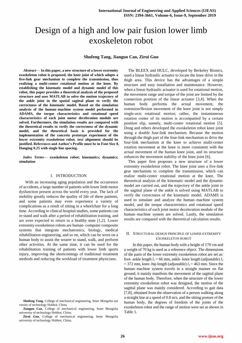
The mechanical structure of the lower extremity

exoskeleton robot designed in this paper is shown in Figure 1,

which includes the backpack device, waist mechanism, hip joint

mechanism, knee joint mechanism, ankle joint mechanism, foot

mechanism, and leggings device, in which the hip and knee

joint mechanism adopt the motor deceleration module active

drive, the ankle joint mechanism and the waist mechanism play

a passive adaptation role, makes the device more comfortable

to wear and flexible in movement.

Figure 1. Mechanical structure of the lower extremity

exoskeleton robot.

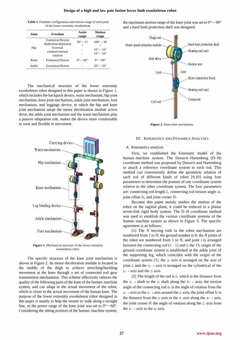
The specific structure of the knee joint mechanism is

shown in Figure 2. Its motor deceleration module is located in

the middle of the thigh to achieve stretching/buckling

movement at the knee through a set of connected rod–gear

transmission mechanisms. This scheme effectively reduces the

quality of the following parts of the knee of the human–machine

system, and can adapt to the actual movement of the robot,

which is closer to the actual movement of the human knee. The

purpose of the lower extremity exoskeleton robot designed in

this paper is mainly to help the wearer to walk along a straight

line, so the power range of the knee joint was set to 0°~−68°.

Considering the sitting position of the human–machine system,

the maximum motion range of the knee joint was set to 0°~−90°

and a hard limit protection shell was designed.

Figure 2. Knee joint mechanism.

III. KINEMATICS AND DYNAMICS ANALYSES

A. Kinematics analysis

First, we established the kinematic model of the

human–machine system. The Denavit–Hartenberg (D–H)

coordinate method was proposed by Denavit and Hartenberg

to attach a reference coordinate system to each rod. This

method can conveniently define the geometric relation of

each rod of different kinds of robot [9,10] using four

parameters to determine the posture of one coordinate system

relative to the other coordinate system. The four parameters

are: connecting rod length li, connecting rod torsion angle αi,

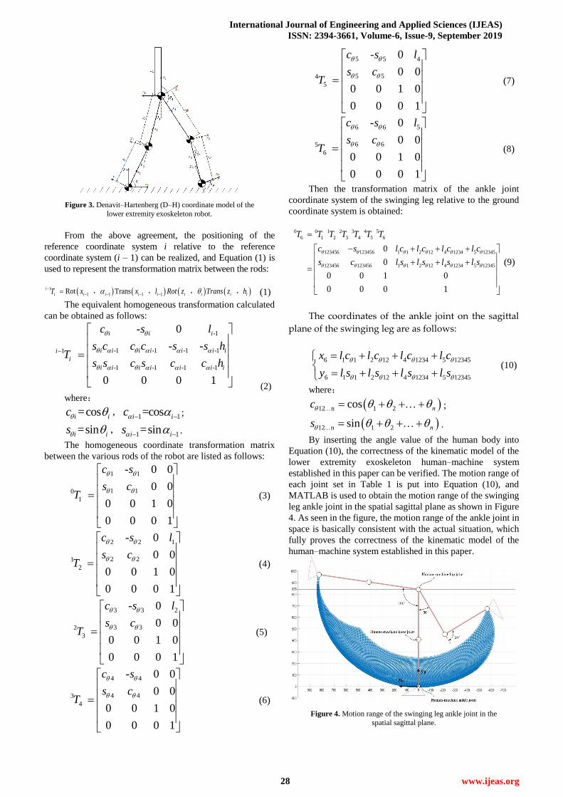
joint offset hi, and joint corner θi. Because this paper mainly studies the motion of the

robot on the sagittal plane, it could be reduced to a planar

seven-link rigid body system. The D–H coordinate method

was used to establish the various coordinate systems of the

human–machine system as shown in Figure 3. The specific

agreement is as follows:

(1) The N moving rods in the robot mechanism are

numbered from 1 to N; the ground number is 0; the N joints of

the robot are numbered from 1 to N, and joint i is arranged

between the connecting rod (i – 1) and i; the O0 origin of the

ground coordinate system is established at the ankle joint of

the supporting leg, which coincides with the origin of the

coordinate system O1; the zi axis is arranged on the axis of

joint i, and the xi − 1 axis is arranged on the cylindrical of the

zi − 1 axis and the zi axis.

(2) The length of the rod is li, which is the distance from

the zi − 1 shaft to the zi shaft along the xi − 1 axis; the torsion

angle of the connecting rod αi is the angle of rotation from the

xi − 1 axis to the zi − 1 axis around the zi axis; the joint offset hi is

the distance from the zi axis to the xi axis along the xi − 1 axis;

the joint corner θi the angle of rotation along the zi axis from

the xi − 1 axis to the xi axis.

International Journal of Engineering and Applied Sciences (IJEAS)

ISSN: 2394-3661, Volume-6, Issue-9, September 2019

28 www.ijeas.org

Figure 3. Denavit–Hartenberg (D–H) coordinate model of the

lower extremity exoskeleton robot.

From the above agreement, the positioning of the

reference coordinate system i relative to the reference

coordinate system (i – 1) can be realized, and Equation (1) is

used to represent the transformation matrix between the rods:

1

1 1 1 1Rot Transi

i i i i i i i i iT x x l Rot z Trans z h

， ， ， ， (1)

The equivalent homogeneous transformation calculated

can be obtained as follows:

-1

-1 -1 -1 -11

-1 -1 -1 -1

- 0

- -

0 0 0 1

i i i

i i i i i i ii

i

i i i i i i i

h

c s l

s c c c s sT

s s c s c c h

(2)

where：

=cosi ic ， 1 1=cos iic ;

=sini is ， 1 1=sin iis .

The homogeneous coordinate transformation matrix

between the various rods of the robot are listed as follows:

1 1

1 10

1

0

0 0

0 0 1 0

0 0 0 1

- 0c s

s cT

(3)

2 2 1

2 21

2

0

0 0

0 0 1 0

0 0 0 1

-c s l

s cT

(4)

3 3

3 3

2

2

3

0

0 0

0 0 1 0

0 0 0 1

-c s l

s cT

(5)

4 4

4 43

4

0

0 0

0 0 1 0

0 0 0 1

- 0c s

s cT

(6)

5 5

5 5

4

4

5

0

0 0

0 0 1 0

0 0 0 1

-c s l

s cT

(7)

6 6 5

6 65

6

0

0 0

0 0 1 0

0 0 0 1

-c s l

s cT

(8)

Then the transformation matrix of the ankle joint

coordinate system of the swinging leg relative to the ground

coordinate system is obtained:

0 0 1 2 3 4 5

6 1 2 3 4 5 6

123456 123456 1 1 2 12 4 1234 5 12345

123456 123456 1 1 2 12 4 1234 5 12345

0

0

0 0 1 0

0 0 0 1

T T T T T T T

c s l c l c l c l c

s c l s l s l s l s

(9)

The coordinates of the ankle joint on the sagittal

plane of the swinging leg are as follows:

6 1 1 2 12 4 1234 5 12345

6 1 1 2 12 4 1234 5 12345

x l c l c l c l c

y l s l s l s l s

(10)

where：

12 n 1 2cos nc ;

12 n 1 2sin ns .

By inserting the angle value of the human body into

Equation (10), the correctness of the kinematic model of the

lower extremity exoskeleton human–machine system

established in this paper can be verified. The motion range of

each joint set in Table 1 is put into Equation (10), and

MATLAB is used to obtain the motion range of the swinging

leg ankle joint in the spatial sagittal plane as shown in Figure

4. As seen in the figure, the motion range of the ankle joint in

space is basically consistent with the actual situation, which

fully proves the correctness of the kinematic model of the

human–machine system established in this paper.

Figure 4. Motion range of the swinging leg ankle joint in the

spatial sagittal plane.

Design of a high and low pair fusion lower limb exoskeleton robot

29 www.ijeas.org

In order to reflect the kinematics characteristics of the

system more accurately, it was also necessary to establish the

kinematic relationship between the knee joint mechanism and

the human–machine system. As shown in Figure 5, the

kinematic model was established on the basis of the motion

diagram of the knee joint mechanism.

Figure 5. Kinematic model of the knee joint mechanism.

As shown in Figure 5, δ1 represents the initial mounting

position angle of rod AF; δ2 is the angle between rod CD and

auxiliary line CE; rod AF is fixed with the output end of the

motor deceleration module; αk indicates the angle at which

rod AF turns relative to its initial position during motion; and

θk indicates the angle at which the calf rod turns relative to the

thigh rod. The relationships among these variables are as

follows:

2tan DE

CD

lζ

l (11)

So,

2 arctan DE

CD

ζl

l (12)

Gears R1 and R2 are respectively fixed to the knee joint

mechanism of the thigh rod and the calf rod, and R1 = R2. In

motion, R2 rotates around R1, and it also rotates around axis

C. The relationship is expressed as follows:

CBC2

kθ' (13)

A planar rectangular coordinate system was established

with A as the original point, as shown in Figure 5, and the

hinge contact coordinates in the figure are:

0

0

A

A

x

y

0

B AB

B

x l

y

cos2

sin2

kC BC AB

kC BC

θx l l

θy l

2

2

cos cos2

sin sin2

E CE k BC AB

E C

k

kE k BC

θx l θ ζ l l

θy l θ ζ l

1

1

cos

sin

F AF k

F AF k

x l α ζ

y l α ζ

due to the relationship expressed below:

2 2

EF E F E Fl x x y y (14)

By substituting the coordinates of Equation (14)

into Equation (12), we obtain:

2

1

2

1

2 cos arctan cos cos2

sin arctan sin sin2

kDEEF CE k BC AB AF k

CD

kDECE k BC AF k

CD

θll l θ l l l α

l

θll θ l l α

l

(15)

From the above analysis, it is assumed that the initial

human–machine system is in an upright state. This is to say,

the calf is collinear with the thigh (i.e., θk = 0°). Then, the size

of each member of the knee joint mechanism is inserted into

Equation (15), and the walking assistance process can be

obtained by calculation and rounding. The angle of rod AF

varies from −38° to −83°, and the angle of the output of the

motor reduction module ranges from 0° to −45°.

B. Dynamics Theory analysis

At present, dynamic analysis methods of multi-rigid

systems are more commonly used, such as the Lagrange

equation method and the Newton–Euler method. The

Lagrange method has the advantages of not requiring internal

force to be solved, simple derivation, and a compact structure,

so the dynamics analysis of external skeletal robots is often

preferred. The Lagrange method is based on the differential of

the energy item to the system variables and time, which takes

the human–machine system as a whole and uses independent

generalized coordinates to complete the establishment of the

system dynamics equation [11].

This article first defines the Lagrange functions of a

multi-rigid system as follows:

T U L E E (16)

where:

ET—the total kinetic energy of the system;

EU—the total potential energy of the system.

Further, using the Lagrange equation for each

generalized coordinate, the general expansion formula of the

kinetic equation can be expressed as follows:

i

i i

d L L

dt q q

(17)

where:

τi—the generalized external force vector (including

force or torque, which depends on the nature of qi; when qi is

the amount of rotation, τi represents the torque, and when qi is

elongated, τi represents the force);

qi—the generalized coordinate vectors.

International Journal of Engineering and Applied Sciences (IJEAS)

ISSN: 2394-3661, Volume-6, Issue-9, September 2019

30 www.ijeas.org

In this paper, the dynamic model of the human–machine

system was first established when the dynamics analysis of the

knee joint mechanism was carried out. Because this paper

mainly focuses on motion on the sagittal plane, the

human–machine system could be reduced to a planar

seven-link rigid system. When the human body walks in a

straight line along a flat surface, the two modes of

single-legged support state and two-legged support state are

included in the gait period according to the contact between

the soles of the feet and the ground. So, two kinetic models

were established in this paper, and the dynamics of the two

different states were analyzed [12].

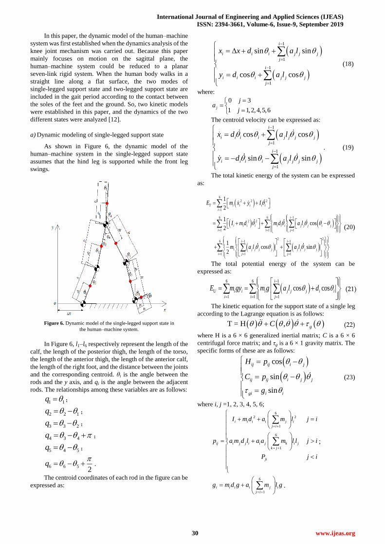
a) Dynamic modeling of single-legged support state

As shown in Figure 6, the dynamic model of the

human–machine system in the single-legged support state

assumes that the hind leg is supported while the front leg

swings.

Figure 6. Dynamic model of the single-legged support state in

the human–machine system.

In Figure 6, l1–l6 respectively represent the length of the

calf, the length of the posterior thigh, the length of the torso,

the length of the anterior thigh, the length of the anterior calf,

the length of the right foot, and the distance between the joints

and the corresponding centroid. θi is the angle between the

rods and the y axis, and qi is the angle between the adjacent

rods. The relationships among these variables are as follows:

1 1q ；

2 2 1q ；

3 3 2q ；

4 3 4q ；

5 4 5q ；

6 6 52

q

.

The centroid coordinates of each rod in the figure can be

expressed as:

1

1

1

1

sin sin

cos cos

i

i i i j j j

j

i

i i i j j j

j

x x d a l

y d a l

(18)

where:

0 3

1 1,2,4,5,6j

ja

j

The centroid velocity can be expressed as:

1

1

1

1

cos cos

sin sin

i

i i i j j ji j

i j

j

i

i i i j j j

j

x d a l

y d a l

. (19)

The total kinetic energy of the system can be expressed

as:

62 2 2

1

6 6 12 2

1 1 1

2 26 1 1

1 1 1

1

2

1cos

2

1cos sin

2

T i i i

i

i

i i i i i j j i j

i i j

i i

i j j j

i i

i i j

j jj j j

i j j

E m y I

I m d m d a l

m a l a

x

l

(20)

The total potential energy of the system can be

expressed as:

6 6 1

1 1 1

cos cos

i

U i i i j j j i i

i i j

E m gy m g a l d (21)

The kinetic equation for the support state of a single leg

according to the Lagrange equation is as follows:

T = H , gC (22)

where H is a 6 × 6 generalized inertial matrix; C is a 6 × 6

centrifugal force matrix; and τg is a 6 × 1 gravity matrix. The

specific forms of these are as follows:

cos

sin

sin

ij ij i j

ij ij i j j

gi i i

H p

C p

g

(23)

where i, j =1, 2, 3, 4, 5, 6;

62 2

1

6

1

i i i i j i

j i

ij i j j i i j k i j

k j

ji

I m d a m l j i

p a m d l a a m l l j i

P j i

;

6

1

i i i i j i

j i

g m d g a m l g

.

Design of a high and low pair fusion lower limb exoskeleton robot

31 www.ijeas.org

As mentioned above, the relationship between qi and θi

can be expressed as:

=X Y q (24)

where:

1 0 0 0 0 0

1 1 0 0 0 0

0 1 1 0 0 0X

0 0 1 1 0 0

0 0 0 1 1 0

0 0 0 0 1 1

；

0

0

0

Y

0

2

.

There is a relationship below:

1X Y q (25)

The expression of each joint moment is:

6 6

1

1 1

T T Xj

i j j jij jiq

(26)

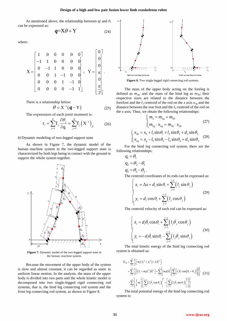
b) Dynamic modeling of two-legged support state

As shown in Figure 7, the dynamic model of the

human–machine system in the two-legged support state is

characterized by both legs being in contact with the ground to

support the whole system together.

Figure 7. Dynamic model of the two-legged support state in

the human–machine system.

Because the movement of the upper body of the system

is slow and almost constant, it can be regarded as static in

uniform linear motion. In the analysis, the mass of the upper

body is divided into two parts and the whole kinetic model is

decomposed into two single-legged rigid connecting rod

systems, that is, the hind leg connecting rod system and the

front leg connecting rod system, as shown in Figure 8.

Figure 8. Two single-legged rigid connecting rod systems.

The mass of the upper body acting on the foreleg is

defined as m3q, and the mass of the hind leg as m3h; their

respective sizes are related to the distance between the

forefoot and the l3 centroid of the rod on the x axis x3q and the

distance between the rear foot and the l3 centroid of the rod on

the x axis. Thus, we obtain the following relationships:

3 3 3

3 3 3 3

q h

q q h h

m m m

m x m x (27)

3 1 1 2 2 3 3

3 5 5 4 4 3 3

sin sin sin

sin sin sin

h h

q q

x x l l d

x x l l d

(28)

For the hind leg connecting rod system, there are the

following relationships:

1 1q

2 2 1q

3 3 2q .

The centroid coordinates of its rods can be expressed as:

1

1

1

1

Δ sin sin

cos cos

i

i i i j j

j

i

i i i j j

j

x x d θ l θ

y d θ l θ

(29)

The centroid velocity of each rod can be expressed as:

1

1

1

1

cos cos

sin sin

i

i i i j j

j

i

i i

i j

i ji j j

j

x d l

y d l

(30)

The total kinetic energy of the hind leg connecting rod

system is obtained as:

32 2 2

T

1

12 2

1 1 1

2 21 1

1 1

3

3

1

3

1

2

1cos

2

1cos sin

2

h i i i

i

i

i i i i i j i j

i i j

i i

i j

i i

i i

j j j

i j j

j

j j

E m y I

I m d m d l θ

x θ

θ θ θ

m l

θ

θ θθ l θ

(31)

The total potential energy of the hind leg connecting rod

system is:

International Journal of Engineering and Applied Sciences (IJEAS)

ISSN: 2394-3661, Volume-6, Issue-9, September 2019

32 www.ijeas.org

3 3 1

U

1 1 1

cos cos

i

h i i i j j i i

i i j

E m gy m g l d (32)

The kinetic equation of the hind leg connecting rod

system obtained by the Lagrange equation is:

T = H ,h h h ghC (33)

In the above equation, Hh is a 3 × 3 generalized inertial

matrix; Ch is a 3 × 3 centrifugal force matrix; and τgh is a 3 × 1

gravity matrix. The specific forms of these are as follows:

˙

cos

sin

sin

ijh ijh i j

ijh ijh i j j

gih ih i

H p

C p

g

(34)

where i, j = 1, 2, 3;

32

1

3

2

1

i i i j i

j i

ijh j j i k i j

k j

jih

I m d m l j i

p m d l m l l j i

P j i

;

1

3

ih i i j i

j i

g m d g m l g .

The relationship between qi and θi is:

Xhq (35)

where：

1 0 0

X 1 1 0

0 1 1

h

.

So, there is: 1Xh q (36)

The expression of each joint movement of the hind leg

connecting rod system is:

1 1

31

3

T T Xj

i j j h jij jiq

(37)

Since the dynamic analysis process of the front leg

connecting rod system is similar to that of the hind leg, there is

no need to repeat it.

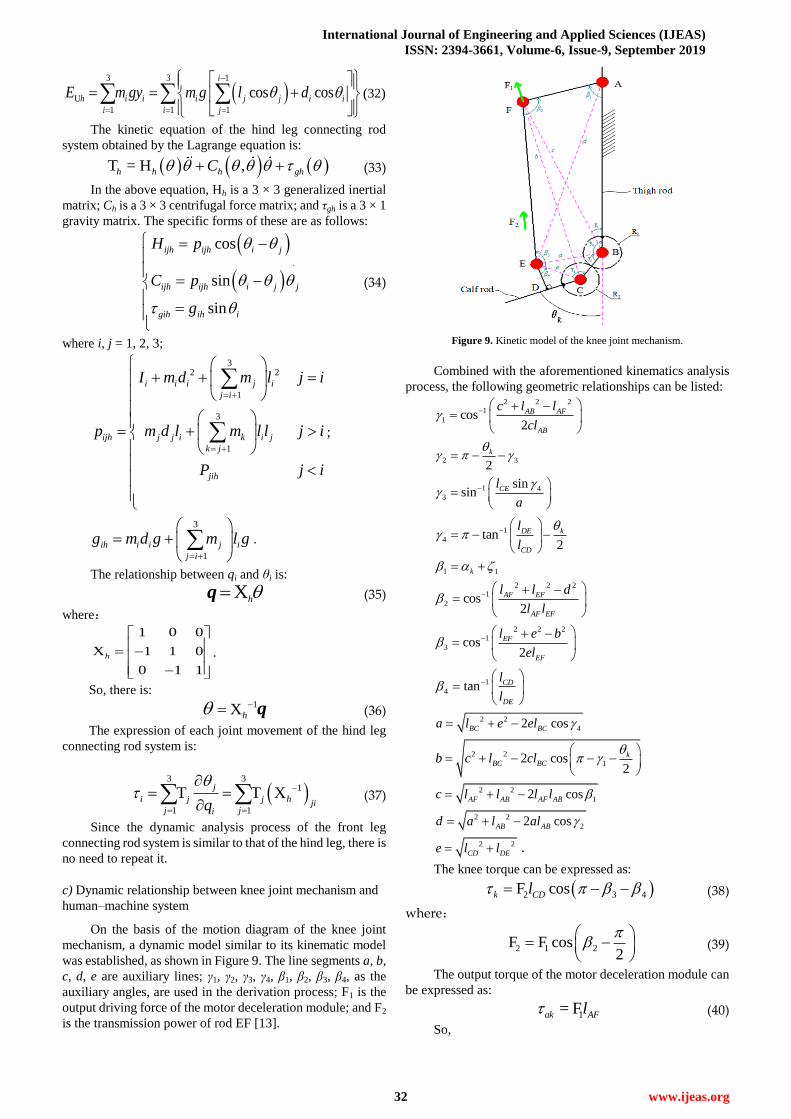
c) Dynamic relationship between knee joint mechanism and

human–machine system

On the basis of the motion diagram of the knee joint

mechanism, a dynamic model similar to its kinematic model

was established, as shown in Figure 9. The line segments a, b,

c, d, e are auxiliary lines; γ1, γ2, γ3, γ4, β1, β2, β3, β4, as the

auxiliary angles, are used in the derivation process; F1 is the

output driving force of the motor deceleration module; and F2

is the transmission power of rod EF [13].

Figure 9. Kinetic model of the knee joint mechanism.

Combined with the aforementioned kinematics analysis

process, the following geometric relationships can be listed: 2 2 2

1

1 cos2

AB AF

AB

c l l

cl

2 32

k

1 4

3

sinsin CEl

a

1

4 tan2

kDE

CD

l

l

1 1k 2 2 2

1

2 cos2

AF EF

AF EF

l l d

l l

2 2

3

21cos

2

EF

EF

l e b

el

1

4 tan CD

DE

l

l

2 2

42 cosBC BCa l e el

2 2

12 cos2

k

BC BCb c l cl

2 2

12 cosAF AB AF ABc l l l l

2 2

22 cosAB ABd a l al

2 2

CD DEe l l .

The knee torque can be expressed as:

2 3 4F cosk CDl (38)

where：

2 1 2F F cos2

(39)

The output torque of the motor deceleration module can

be expressed as:

1= Fak AFl (40)

So,

Design of a high and low pair fusion lower limb exoskeleton robot

33 www.ijeas.org

2 3 4

=

cos cos2

AF kak

CD

l

l

(41)

C. Kinematics and Dynamics Simulations

The three-dimensional structure model of the

human–machine system of the lower extremity exoskeleton

was introduced into ADAMS, where the model structure was

simplified. The material of each component was set to

aluminum alloy, with a density of 2.82 × 103 kg/m3; the

Young's modulus was 7.2 × 104 MPa; and the Poisson's ratio

was 0.33. Then, according to the motion principle of the

model structure, the corresponding motion pairs and drivers

were added. In this paper, the output angle spline data of the

lower extremity hip angle spline data and the first kinematics

analysis obtained by MATLAB were imported into ADAMS

as the driving functions of the hip and knee joint of the

exoskeleton robot when it walks in a straight line on a flat

surface at a speed of 0.8 m/s. The kinematics and dynamics

simulations of the human–machine system model were

carried out, and the simulation motion process is shown in

Figure 10.

Figure 10. Simulation motion process of the human–machine

system based on ADAMS.

After simulation and filtering processing, the

torque–time relation curves of each joint of the lower

extremity robot were obtained, and these results were

compared with the theoretical calculation results through

MATLAB, as shown in Figures 11 and 12.

（a）Left-Hip

（b）Right-Hip

Figure 11. Hip torque–time relation curve.

（a）Left-Knee

（b）Right-Knee

Figure 12. Knee torque–time relation curve.

As can be seen from Figures 11 and 12, the simulation

results of the torque–time curve of each joint were somewhat

biased in comparison to the theoretical calculation results, but

the deviation range was small and can be regarded as

reasonable deviation, so the correctness of the

aforementioned dynamic analysis model was proved. The

analysis of the causes of the deviation may possibly be due to

the fact that we did not take into account the friction between

the components when we performed the theoretical analysis

of the human–machine system, nor did we consider the

friction and contact force between the human and the machine

and the friction and contact force between the

human–machine system and the ground. As a result, the

theoretical analysis model was too idealistic. Moreover, the

simulation process of the structure may also have caused

deviations from the theoretical analysis.

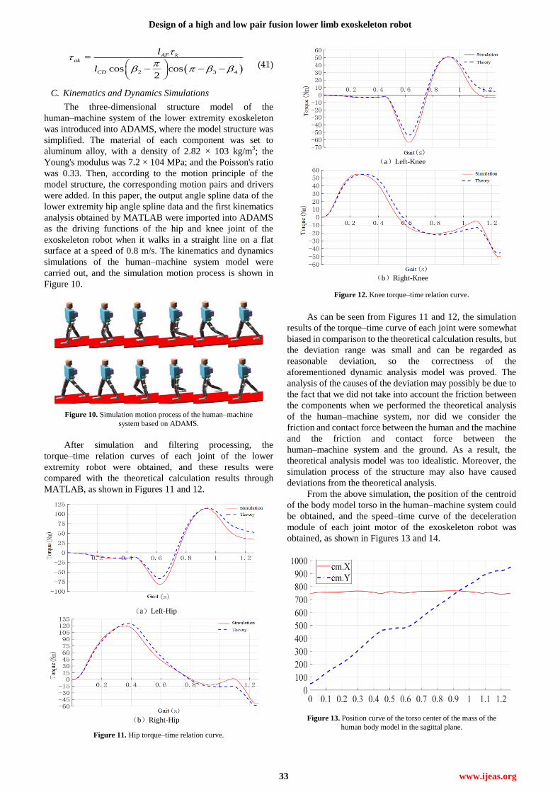
From the above simulation, the position of the centroid

of the body model torso in the human–machine system could

be obtained, and the speed–time curve of the deceleration

module of each joint motor of the exoskeleton robot was

obtained, as shown in Figures 13 and 14.

Figure 13. Position curve of the torso center of the mass of the

human body model in the sagittal plane.

International Journal of Engineering and Applied Sciences (IJEAS)

ISSN: 2394-3661, Volume-6, Issue-9, September 2019

34 www.ijeas.org

（a）Hip

（b）Knee

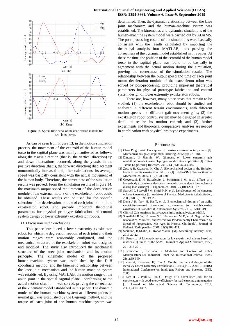
Figure 14. Speed–time curve of the deceleration module for

each joint motor.

As can be seen from Figure 13, in the motion simulation

process, the movement of the centroid of the human model

torso in the sagittal plane was mainly manifested as follows:

along the x axis direction (that is, the vertical direction) up

and down fluctuations occurred; along the y axis in the

positive direction (that is, the forward direction) displacement

monotonically increased and, after calculations, its average

speed was basically consistent with the actual movement of

the human body. Therefore, the correctness of the simulation

results was proved. From the simulation results of Figure 14,

the maximum output speed requirement of the deceleration

module of the external motors of the exoskeleton robot could

be obtained. These results can be used for the specific

selection of the deceleration module of each joint motor of the

exoskeleton robot, and provide important theoretical

parameters for physical prototype fabrication and control

system design of lower extremity exoskeleton robots.

D. Discussion and Conclusions

This paper introduced a lower extremity exoskeleton

robot, for which the degrees of freedom of each joint and their

motion ranges were reasonably configured, and the

mechanical structure of the exoskeleton robot was designed

and modeled. The study also introduced the mechanical

structure of the knee joint mechanism and its motion

principle. The kinematic model of the proposed

human–machine system was established by the D–H

coordinate method, and the kinematic relationship between

the knee joint mechanism and the human–machine system

was established. By using MATLAB, the motion range of the

ankle joint in the spatial sagittal plane—conforming to the

actual motion situation—was solved, proving the correctness

of the kinematic model established in this paper. The dynamic

model of the human–machine system at different points in

normal gait was established by the Lagrange method, and the

torque of each joint of the human–machine system was

determined. Then, the dynamic relationship between the knee

joint mechanism and the human–machine system was

established. The kinematics and dynamics simulations of the

human–machine system model were carried out by ADAMS.

The post-processing results of the simulations were basically

consistent with the results calculated by importing the

theoretical analysis into MATLAB, thus proving the

correctness of the dynamic model established in this paper. At

the same time, the position of the centroid of the human model

torso in the sagittal plane was found to be basically in

agreement with the actual motion during the simulation,

proving the correctness of the simulation results. The

relationship between the output speed and time of each joint

motor deceleration module of the exoskeleton robot was

solved by post-processing, providing important theoretical

parameters for physical prototype fabrication and control

system design of lower extremity exoskeleton robots.

There are, however, many other areas that remain to be

studied: (1) the exoskeleton robot should be studied and

analyzed in different terrain environments, with different

motion speeds and different gait movement gaits; (2) the

exoskeleton robot control system may be designed in greater

detail to realize its motion control; and (3) further

experiments and theoretical comparative analyses are needed

in combination with physical prototype experiments.

.

REFERENCES

[1] Chen Ping, quiet. Conception of passive exoskeleton in patients [J].

Mechanical design & amp; manufacturing, 2012 (6): 279-281.

[2] Dingmin, Li Jianmin, Wu Qingwen, et. Lower extremity gait

rehabilitation robot: research progress and clinical application [J]. China

Tissue Engineering Research, 2010, 14 (35): 6604-6607.

[3] Zoss A B, Kazerooni H, Chu A. Biomechanical design of the Berkeley

lower extremity exoskeleton (BLEEX)[J]. IEEE/ASME Transactions on

Mechatronics, 2006, 11(2):128-138.

[4] Gregorczyk K N, Hasselquist L, Schiffman J M, et al. Effects of a

lower-body exoskeleton device on metabolic cost and gait biomechanics

during load carriage[J]. Ergonomics, 2010, 53(10):1263-1275.

[5] Scarvell J, Scarvell J M, Smith K N, et al. Development of the concepts

of knee kinematics [J]. Archives of Physical Medicine & Rehabilitation,

2003, 84(12):1895-1902.

[6] Dong J H, Park H, Ha T, et al. Biomechanical design of an agile,

electricity-powered lower-limb exoskeleton for weight-bearing

assistance [J]. Robotics & Autonomous Systems, 2017, 95:181-195.

[7] Clinical Gait Analysis. http://www.clinicalgaitanalysis.com/[OL].

[8] Stansfield B W, Hillman S J, Hazlewood M E, et al. Sagittal Joint

Kinematics, Moments, and Powers Are Predominantly Characterized by

Speed of Progression, Not Age, in Normal Children[J]. Journal of

Pediatric Orthopaedics, 2001, 21(3):403-411.

[9] Siciliano, B,Khatib, O. Robot Manual [M]. Machinery industry Press,

2013:20-22.

[10] Denavit J. A kinematic notation for lower-pair mechanisms based on

matrices [J]. Trans. of the ASME. Journal of Applied Mechanics, 1955,

22：215-221.

[11] Sciavicco L, Siciliano B. Modeling and Control of Robot

Manipu-lators [J]. Industrial Robot An International Journal, 1996,

21(1):99-100.

[12] Zoss A, Kazerooni H, Chu A. On the mechanical design of the

Berkeley Lower Extremity Exoskeleton (BLEEX)[C]// 2005 IEEE/RSJ

International Conference on Intelligent Robots and Systems. IEEE,

2005.

[13] Kim H G, Park S, Han C. Design of a novel knee joint for an

exoskeleton with good energy efficiency for load-carrying augmentation

[J]. Journal of Mechanical Science & Technology, 2014,

28(11):4361-4367.