Design Evaluation of a Particle Bombardment System Used to ...

Copyright © 2014 Tech Science Press CMES, vol.98, no.2, pp.221-245, 2014

Design Evaluation of a Particle Bombardment SystemUsed to Deliver Substances into Cells

Eduardo M. B. Campello1,2 and Tarek I. Zohdi3

Abstract: This work deals with the bombardment of a stream of particles pos-sessing varying mean particle size, velocity and aspect ratio into a cell that has fixed(known) compliance characteristics. The particles are intended to penetrate the cellmembrane causing zero or minimum damage and deliver foreign substances (whichare attached to their surfaces) to the interior of the cell. We adopt a particle-based(discrete element method) computational model that has been recently developedby the authors to describe both the incoming stream of particles and the cell mem-brane. By means of parametric numerical simulations, treating the stream’s meanparticle size, velocity and aspect ratio as random variables, we explore the synergybetween these parameters and identify basic trends as to how changes in the inputparameters affect the output results, and as to what are the best combinations ofparameter values that lead to (i) the highest amount of particle delivery and (ii) thelowest level of membrane damage. Conclusions are drawn on this regard basedon statistical assessment of the simulations results. Computational particle-basedmodels render reliable and fast simulation tools. We believe they can be very usefulto help advance the design of particle bombardment systems.

Keywords: particle bombardment guns; design evaluation; cells; drug delivery;particle methods; discrete element methods.

1 Introduction

Modern cell biology makes extensive use of delivery mechanisms to deliver foreignsubstances into cells. Proteins, drugs, genetic material, biological stains, and many

1 Dept. Structural and Geotechnical Engineering, University of São Paulo, P.O. Box 61548, 05424-970, São Paulo, SP, Brazil. Email: [email protected]

2 Current temporary address: Dept. Mechanical Engineering, University of California at Berkeley.6195 Etcheverry Hall, Berkeley, CA, 94720-1740, USA. Tel: +1 (510) 612-3658, Email: [email protected].

3 Dept. Mechanical Engineering, University of California at Berkeley, 6195 Etcheverry Hall, 94720-1740, Berkeley, CA, USA. Email: [email protected]

222 Copyright © 2014 Tech Science Press CMES, vol.98, no.2, pp.221-245, 2014

other materials are often desired to be transported to the interior of cells to under-take a specific task. The cell membrane (in case of plant cells, also the cell wall)constitutes the main physical barrier in this regard. Among the existing technolo-gies to accomplish such transport, particle bombardment guns have been preferredin recent years in many applications. This is partly due to their ability to deal withcells both in vitro and in vivo (i.e., cells either in suspension or in their natural en-vironment) and with groups of cells simultaneously (instead of only single cells ata time). Particle guns consist of a channeled accelerator that shoots single parti-cles or streams of particles of a noble, inert material (usually gold or tungsten) towhich the desired foreign substances are attached. They were first introduced bySanford and coworkers in the late 1980s (see the seminal papers [Sanford, Klein,Wolf and Allen (1987)] and [Klein, Wolf, Wu and Sanford (1987)]), and rely on avery simple principle: if the incoming particles have the appropriate sizes and areaccelerated to the appropriate velocities, they should readily penetrate thin barrier-s such as cell walls and cell membranes, thereby entering the cell cytoplasm. Theidea is schematically illustrated in Fig. 1, where typical dimensions are also shown.

In the design of particle guns, the lipid bilayer structure of the cell membrane isa primary aspect to be considered. Lipid molecules can be idealized as a spher-ical polar head (representing a phosphoric group) that has one or two elongatedtails (representing hydrocarbon, fatty acid chains). In aqueous media, they orga-nize themselves into various types of structures due to their amphiphilic properties(the polar heads are hydrophilic, the hydrocarbon chains are hydrophobic), oneof which is the two-layer formation that is observed in cellular membranes. Theforces that hold them together in such arrangement are not due to strong covalen-t or ionic bonds, but instead arise from weaker van der Waals, hydrophobic andhydrogen-bonding interactions. This aspect provides the membrane a very soft,flexible, almost fluid-like behavior, and yet good response to both stretching andbending deformations are observed (along with excellent selective permeability).The transport of substances across the membrane barrier by means of particle bom-bardment guns is greatly governed by the mechanical characteristics of this struc-ture.

This work deals with the computational modeling of particle bombardment gunsand aims at establishing a basic framework for design evaluation of these types ofdelivery mechanisms. We use a particle-based (discrete element method) model re-cently proposed by the authors in [Campello and Zohdi (2014)] to describe both theincoming stream of particles and the cell membrane, and perform parametric simu-lations of the system by making the stream’s mean particle size, velocity and aspectratio as design parameters. More specifically, these parameters are treated as ran-dom variables whose values are sampled from underlying probability distribution

Design Evaluation of a Particle Bombardment System 223

lipid 2 nm

stream of particles

cell membrane (lipid bilayer)

cell length 100 nm

cell

10 nm

Figure 1: Schematic of a particle bombardment gun for the delivery of substancesinto a cell.

functions, with which we construct several sets of design vectors. Each design vec-tor generates a computational particle problem that is then solved numerically withour particle solver. In this latter, the compliance of the cell is taken into account byusing an appropriate (yet simple) model of the lipid’s bonding interactions, togetherwith consideration of the cell internal pressure. Both the bonding and internal pres-sure parameters are assumed to be known and held with fixed values on all analyses.Two measures (or indicators of performance) are defined to quantify respectivelythe delivery success and the membrane damage associated with each design vectoror simulation. After performing all simulations, we compute the mean value, stan-dard deviation and coefficients of variation of the design parameters and of the twodefined measures. We also compute the correlation coefficients of the two mea-sures with respect to each of the design parameters. These statistics allow us tomake interpretations such as how variabilities in the input parameters propagate tothe output results, and what are the best combinations of parameter values that leadto (i) the highest amount of particle delivery and (ii) the lowest level of membranedamage. Other basic trends in the system can also be identified.

It is evident that there are multiple parameters that govern the response of cellsagainst the impact by a stream of particles. Yet, with the aim of solely establish-ing a framework for rapid parametric investigations for design evaluation, and ofshowing how the synergy of parameters can be identified, here we work only withthe three parameters stated above. We must mention, moreover, that there existsa number of other theoretical and/or computational approaches that could be usedto study the transport of substances across the cell membrane, such as stochasticdynamics [Wang, Sigurdsson, Brandt and Atzberger (2013); Pastor and Venable(1993)], Monte Carlo simulations [Hac, Seeger, Fidorra and Heimburg (2005);Pastor (1994)], molecular dynamics models [Tieleman, Marrink and Berendsen(1997); Delemotte and Tarek (2012); Andoh, Okazaki and Ueoka (2013)], mean


field models [Khelashvili, Weinstein and Harries (2008)], continuum mechanicsmodels with spatial discretizations [Rangamani, Agrawal, Mandadapu, Oster andSteigmann (2013)], etc., to name just a few. Yet, at the tens of nano- to a few micro-time and length scales, we believe that particle-based models are the most suitedwhen one is interested in the overall, collective behavior of the system. They al-low for simpler representations of the whole cell and incoming substances (with noneed for detailed descriptions of the complex short-range forces that act betweenthe polar headgroups and hydrocarbon chains of the lipid molecules). Also, multi-ple contact/impact with the opening of localized holes on the membrane (localized“rupture”) is straightforward to characterize. They allow for the construction ofrapid simulation tools. With such tools, particle bombardment guns can be morethoroughly designed and tested without the need to resort to a great number ofphysical experiments. Physical experiments can be expensive and time consum-ing when dealing with cells, and the number of parameters that can be adjustedwithin feasible cost and time is very limited when compared to computational in-vestigations. For details on particle methods, see e.g. [Bicanic (2004); Pöschel andSchwager (2004); Duran (1997)].

The paper is organized as follows: in Section 2 we present an overview of the e-quations that govern the dynamics of particle systems, with emphasis on the severaltypes of mechanical forces involved herein and their representations; in Section 3we present a brief description of the particle model adopted here for the cell mem-brane, which is taken from [Campello and Zohdi (2014)]; in Section 4 we give anoutline of our numerical solution scheme to the system’s equations; in Section 5we show how we construct the design vectors and the associated particle problem-s, perform the corresponding numerical simulations, and extract the simulations’results and statistics; and in Section 6 we derive our conclusions.

Throughout the text, plain italic letters (a,b, . . . ,α,β , . . . ,A,B, . . .) denote scalarquantities, whereas boldface italic ones (aaa,bbb, . . . ,ααα,βββ , . . . ,AAA,BBB, . . .) denote vectorsin a three-dimensional Euclidean space. The inner product of two vectors is denotedby

uuu · vvv = u1v1 +u2v2 +u3v3 , (1)

where ui and vi (i = 1,2,3) are the corresponding three components of the vectors,and the norm of a vector by

‖uuu‖=√

uuu ·uuu =√

u21 +u2

2 +u23 . (2)


2 Dynamics of Particle Systems

The primary assumption in the computational model that we use is that both theincoming substances and the lipid molecules of the cell membrane are a collectionof spherical particles forming a discrete dynamical system. A purely mechanistic(Newtonian) description is then followed (biological and chemical effects are notconsidered). The particles are assumed to be small enough so that the effect oftheir rotations with respect to their center of mass is unimportant to their overallmotion. Permanent deformations due to contact and collisions are supposed to beminor and thereby ignored, which means that all particles remain spherical and withconstant radius throughout. Effects of temperature changes are also considered tobe irrelevant – although these can be easily incorporated, following e.g. the schemeproposed in [Zohdi (2012)].

Let the system be comprised of Np particles, each one with known mass mi andknown radius Ri (i = 1, ...,Np), and let us denote the position vector of a particleby rrri, the velocity vector by vvvi and the acceleration vector by aaai. According toNewton’s second law, at every time instant t the following equation must hold foreach particle:

miaaai = fff toti , (3)

where fff toti is the total force vector acting on the particle. This vector is made up of

the sum of four force contributions as follows

fff toti = fff env

i + fff bondi + fff con

i + fff f rici , (4)

in which fff envi comprises the forces due to the environment (they represent the ef-

fects of the surrounding media or fluid on the particle), fff bondi are the forces due

to bonding or adhesive interactions with other particles, fff coni the forces due to me-

chanical contact (or collisions) with other particles and/or obstacles, and fff f rici the

forces due to friction that arise from these contacts or collisions.

The forces due to the environment are given by

fff envi = miggg+ fff pres

i + fff dragi , (5)

where ggg is the external (i.e. environmental) gravity field, fff presi is the pressure force

and fff dragi is the drag force, both due to the surrounding fluid. In this work, the

pressure force has a given magnitude whereas the drag force is given by followingsimple model, which constitutes a source of damping for the system:

fff dragi =−cenv(vvvi− vvvenv) , (6)


where cenv is a damping parameter and vvvenv is the (local) velocity of the surroundingfluid. One should notice that this scheme constitutes a one-way-only kind of cou-pling between the fluid and the particle, in the sense that the fluid affects the particlebut the particle does not affect the fluid (more elaborate, fully coupled models canbe constructed if necessary, although this increases drastically the complexity ofthe solution scheme, since the fluid local velocity and pressure fields need to be in-troduced as additional variables). Other environmental forces could be consideredin (5), such as electric forces due to external electric fields, magnetic forces due toexternal magnetic fields, etc., but these are not considered in the present work.

The forces due to bonding or adhesive interactions with other particles are given by

fff bondi =

Nb

∑j=1

fff bondi j , (7)

where Nb is the number of particles that are bonded to particle i and fff bondi j is the

(binary) bonding force that acts between particle i and particle j. This force has thegeneral expression

fff bondi j = Ki jnnni j , (8)

in which Ki j is a parameter dictating the intensity of the bonding for the pair {i, j}and nnni j is the unit vector that points from the center of particle i to the center ofparticle j, i.e.,

nnni j =rrr j− rrri∥∥rrr j− rrri

∥∥ . (9)

Vector nnni j will be from now on referred to as the pair’s central direction. Scalar Ki j

can be modeled in a number of ways, such as by using a combination of attractiveand repulsive force coefficients that are functions of the distance between the par-ticles [Zohdi (2012)] (this can be understood as derived from a generalized Mie’spotential, of which the classical Lennard-Jones potential [Lennard-Jones (1924)] isa special case), by using surface energy arguments [Johnson, Kendall and Roberts(1971); Israelachvili (2011)], direct van de Waals effects, etc. In Section 3 we showthe model that we adopt for the purpose of this work, which was introduced by theauthors in [Campello and Zohdi (2014)] (see also [Campello (2014)]) and is basedon the presence of a fictitious spring-dashpot device connecting particles i and j.

The forces due to contact and collisions with other particles are modeled here withan overlap-based scheme. Accordingly, the contact force is assumed to be a func-tion of the amount of geometrical overlap or penetration (i.e., “deformation”) be-tween the particles in contact. We follow Hertz’s elastic contact theory (see e.g.


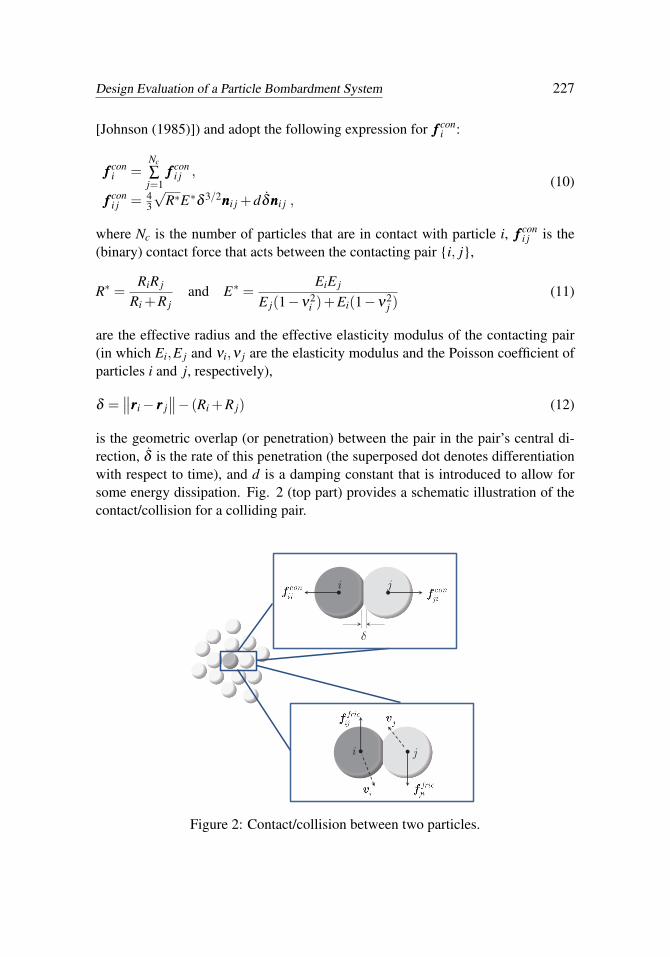
[Johnson (1985)]) and adopt the following expression for fff coni :

fff coni =

Nc

∑j=1

fff coni j ,

fff coni j = 4

3

√R∗E∗δ 3/2nnni j +dδ̇nnni j ,

(10)

where Nc is the number of particles that are in contact with particle i, fff coni j is the

(binary) contact force that acts between the contacting pair {i, j},

R∗ =RiR j

Ri +R jand E∗ =

EiE j

E j(1−ν2i )+Ei(1−ν2

j )(11)

are the effective radius and the effective elasticity modulus of the contacting pair(in which Ei,E j and νi,ν j are the elasticity modulus and the Poisson coefficient ofparticles i and j, respectively),

δ =∥∥rrri− rrr j

∥∥− (Ri +R j) (12)

is the geometric overlap (or penetration) between the pair in the pair’s central di-rection, δ̇ is the rate of this penetration (the superposed dot denotes differentiationwith respect to time), and d is a damping constant that is introduced to allow forsome energy dissipation. Fig. 2 (top part) provides a schematic illustration of thecontact/collision for a colliding pair.

i j

i j

Figure 2: Contact/collision between two particles.


The damping constant d is taken here following the ideas of [Wellmann and Wrig-gers (2012)], which means

d = 2ξ

√2√

R∗E∗m∗δ 1/4 , (13)

wherein ξ is the damping rate of the collision (which must be specified) and m∗ isthe effective mass of the colliding pair, i.e.,

m∗ =mim j

mi +m j. (14)

The damping rate ξ enables us to enforce the type of energy dissipation that shalloccur during the collision in the pair’s central direction. If the colliding pair is seenas a one-dimensional spring-dashpot system (SDS) of mass m∗ and damping rateξ , its dynamics can be fully controlled by specifying appropriate ξ ’s. Recallingthe solution to a vibration problem of a 1-D SDS, it follows that: (1) when ξ = 0,no damping exists and the collision is a perfectly elastic, energy-conserving one(undamped SDS); (2) when 0 < ξ < 1, small to moderate damping exists and en-ergy dissipation occurs at small to moderate rates (underdamped SDS); (3) whenξ = 1, strong damping exists and rapid energy dissipation is observed (criticallydamped SDS); and (4) when ξ > 1, very strong damping with rapid dissipation isobserved (overdamped SDS). Equation (13) is a generalization of the ideas pro-posed by Cundall and Strack in their seminal work [Cundall and Strack (1979)],wherein only critically damped collisions were considered.

The forces due to friction, which arise from the contacts/collisions, are modeledby assuming that the friction coefficients of all colliding pairs are small enough sothat a continuous slide (with an opposing dynamic friction force) is to be expectedduring the entire duration of the contact/collision (see Fig. 2, bottom part). By“continuous slide” we mean that there is to be no stick between the contacting pair.Although a stick-slip model could be considered, we find it to be unnecessary forthe problem that we are concerned with in this work. Thereby, here we write

fff f rici =

Nc

∑j=1

fff f rici j ,

fff f rici j = µd

∥∥ fff coni j

∥∥τττ i j ,

(15)

where fff f rici j is the (binary) friction force that acts between the colliding particles i

and j, µd is the coefficient of dynamic friction for the colliding pair, and

τττ i j =vvv jt − vvvit∥∥vvv jt − vvvit

∥∥ (16)


is the tangential direction of the contact/collision, which is the direction of thetangential relative velocity of i and j, in which

vvvit = vvvi− (vvvi ·nnni j)nnni j

vvv jt = vvv j− (vvv j ·nnni j)nnni j .(17)

3 Particle Model for the Cell Membrane

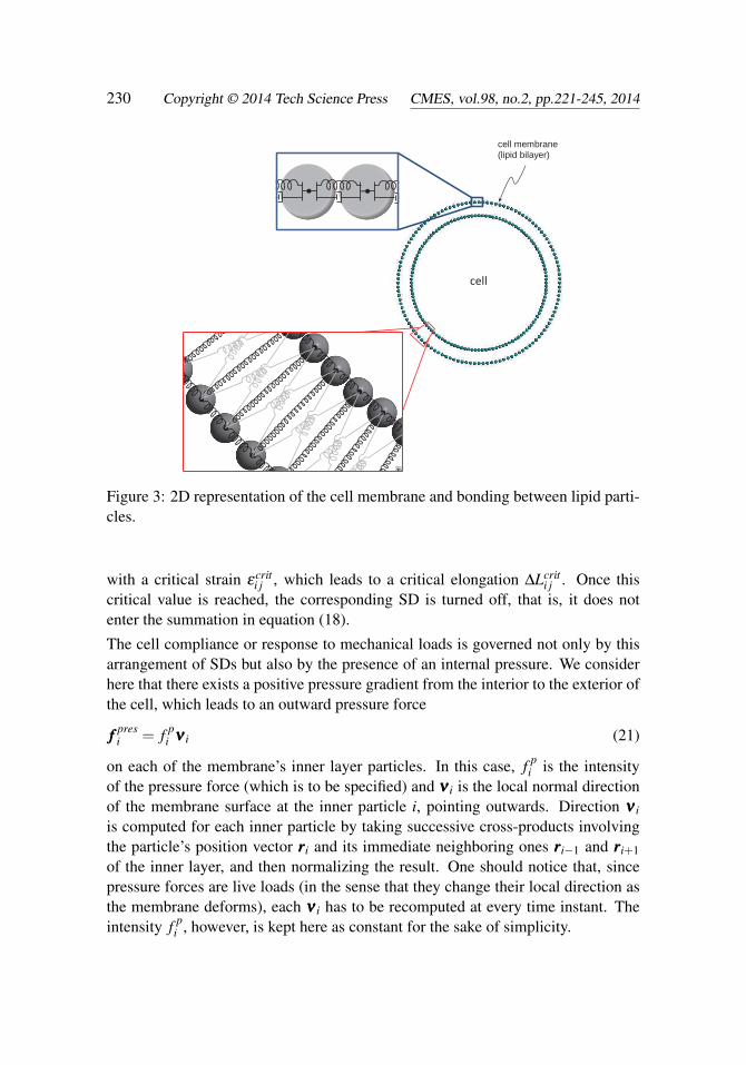
We follow the membrane model that has been proposed by the authors in [Campelloand Zohdi (2014)] and adopt a two-dimensional, circular-shaped idealization of thecell, as depicted in Fig. 3 (a fully three-dimensional one can be considered withoutany modification, at the only expense of having more particles in the system). Forsimplicity, the presence of other substances on the membrane surface rather thanlipids (proteins, sugars, cholesterols, etc.) is ignored. Within this setting, each lipidmolecule is represented by a spherical particle (corresponding to the molecule’sheadgroup) that is bonded to its neighboring ones of the same layer by means ofspring-dashpots (SDs), as indicated in the upper zoom of Fig. 3. To capture the“through-the-thickness” or “transverse” bonding that maintains the two layers to-gether (which is in great part due to hydrophilic/hydrophobic interactions with thesurrounding aqueous media), transversal SDs are placed connecting particles in thecell’s radial direction. And to account for circumferential interactions between thetwo layers, crosswise SDs are introduced. The scheme is as depicted in the lowerzoom of Fig. 3, where the dashpots are not shown for the sake of clarity. Each SDhas stiffness ki j, damping constant ci j and initial length L0i j.

Accordingly, on each particle i of the membrane there act five bonding forces,corresponding to the five SDs that are connected to i. This allows us to write, foreach of these particles:

fff bondi =

5∑j=1

fff bondi j ,

fff bondi j = ki j∆Li jnnni j− ci j(vin− v jn)nnni j ,

(18)

where

∆Li j =∥∥rrri− rrr j

∥∥−L0i j (19)

is the elongation of the spring that connects particles i and j and

vin = vvvi ·nnni j and v jn = vvv j ·nnni j (20)

are the central components of the particles’ velocities. To allow for the bonds tobreak (rupture) if the particles are pulled apart strongly enough, each SD is provided


cell

cell membrane (lipid bilayer)

Figure 3: 2D representation of the cell membrane and bonding between lipid parti-cles.

with a critical strain εcriti j , which leads to a critical elongation ∆Lcrit

i j . Once thiscritical value is reached, the corresponding SD is turned off, that is, it does notenter the summation in equation (18).

The cell compliance or response to mechanical loads is governed not only by thisarrangement of SDs but also by the presence of an internal pressure. We considerhere that there exists a positive pressure gradient from the interior to the exterior ofthe cell, which leads to an outward pressure force

fff presi = f p

i ννν i (21)

on each of the membrane’s inner layer particles. In this case, f pi is the intensity

of the pressure force (which is to be specified) and ννν i is the local normal directionof the membrane surface at the inner particle i, pointing outwards. Direction ννν i

is computed for each inner particle by taking successive cross-products involvingthe particle’s position vector rrri and its immediate neighboring ones rrri−1 and rrri+1of the inner layer, and then normalizing the result. One should notice that, sincepressure forces are live loads (in the sense that they change their local direction asthe membrane deforms), each ννν i has to be recomputed at every time instant. Theintensity f p

i , however, is kept here as constant for the sake of simplicity.


One important aspect in this membrane model is how to come up with appropriatevalues for the springs’ stiffnesses. As proposed in [Campello and Zohdi (2014)],here we estimate their values from surface tension arguments, since the value ofthe surface tension (or interfacial free energy per unit area) for hydrocarbon-waterinterfaces is well documented in the literature. This is reported as being around 50mJ/m2 for monolayers (although the presence of the hydrophilic headgroup mayreduce it to something closer to 20 mJ/m2, see e.g. [Israelachvili (2011)]), so thatfor bilayers it must be multiplied by two. We check the obtained value against theone that follows from the (more or less known) maximum internal pressure that thecell can undergo before membrane rupture. From static equilibrium arguments onone isolated particle, one can equate the force due to this internal pressure to theresultant (in the radial direction) of the forces of the springs that are connected tothe particle. By assuming that all springs have the same stiffness, ki j follows.

The reader should notice in this model that, since each lipid bonding is assumedto behave according to a one-dimensional constitutive relation, more complex lawssuch as nonlinear hyperelasticity with progressive damage and rupture (allowingfor non-abrupt breaking of the bonds) can be straightforwardly considered.

Remark 1. It is important to notice the role of the crosswise SDs. They can beunderstood as arising from the small lateral interactions that exist between the hy-drocarbon chains of adjacent lipid molecules. Their presence is crucial in providinga combined bending behavior for the two layers. Not having them causes each layerto deform as independent sheets upon bending, which is not a realistic behavior.

Remark 2. For a pair of bonded (neighboring) lipid molecules, the spring stiffnesski j and the dashpot constant ci j can be understood as “homogenized” propertiesthat represent the overall (average) behavior of the intermolecular interactions be-tween the two molecules. In fact, we believe that many of the physical propertiesof the cell membrane can be qualitatively described without the need to resort todetailed representations of the complex short-range forces that act between the po-lar headgroups and hydrocarbon chains of its lipid molecules. In an analogy withgas-liquid phase interactions in thermodynamics, for example, the classical van derWaals equation of state contains no information on the characteristics and rangeof intermolecular forces, and yet renders a very satisfactory representation of thephase behavior.

4 Time Integration Scheme for Solution of the System’s Dynamics

For the solution of the system’s dynamics, we start by considering the accelerationvector aaai of each particle, which may be computed from equation (3). By definition,


this vector also follows from the time-continuous differential equation

dvvvi

dt= aaai . (22)

Integration of (22) between time instants t and t +∆t, together with (3), furnishes

vvvi(t +∆t) = vvvi(t)+1mi

∫ t+∆t

tfff tot

i dt . (23)

The integral on the right-hand side of (23) is difficult (if not impossible) to beevaluated analytically because of the intricate dependence of fff tot

i with time. A nu-merical approximation is thus necessary and here we adopt the following scheme,which corresponds to the use of a generalized trapezoidal rule:∫ t+∆t

tfff tot

i dt ≈[φ fff tot

i (t +∆t)+(1−φ) fff toti (t)

]∆t , (24)

with 0 ≤ ϕ ≤ 1. If φ = 0, the integration corresponds to an (explicit) forwardEuler scheme; if φ = 1, to an (implicit) backward Euler one; and if φ = 0.5, to the(implicit) classical trapezoidal rule. By inserting (24) into (23), one has

vvvi(t +∆t) = vvvi(t)+∆tmi

[φ fff tot


]. (25)

On the other hand, by definition the velocity vector vvvi of each particle is related tothe particle’s position by the time-continuous differential equation

drrri

dt= vvvi . (26)

This equation can also be integrated between t and t +∆t, yielding

rrri(t +∆t) = rrri(t)+∫ t+∆t

tvvvidt . (27)

The integral in (27) is also difficult to be evaluated analytically, and then we adoptthe following approximation, similarly to what was done in (24):∫ t+∆t

tvvvidt ≈ [φvvvi(t +∆t)+(1−φ)vvvi(t)]∆t . (28)

By introducing (28) into (27), one arrives at

rrri(t +∆t) = rrri(t)+ [φvvvi(t +∆t)+(1−φ)vvvi(t)]∆t . (29)


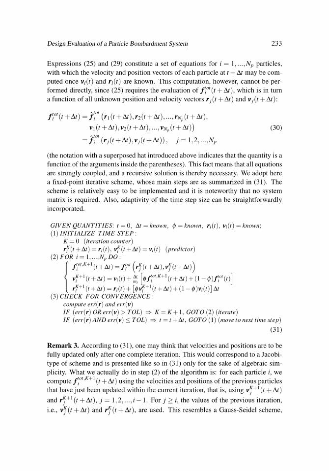
Expressions (25) and (29) constitute a set of equations for i = 1, ...,Np particles,with which the velocity and position vectors of each particle at t +∆t may be com-puted once vvvi(t) and rrri(t) are known. This computation, however, cannot be per-formed directly, since (25) requires the evaluation of fff tot

i (t +∆t), which is in turna function of all unknown position and velocity vectors rrr j(t +∆t) and vvv j(t +∆t):

fff toti (t +∆t) = f̂ff

toti(rrr1(t +∆t),rrr2(t +∆t), ...,rrrNp(t +∆t),

vvv1(t +∆t),vvv2(t +∆t), ...,vvvNp(t +∆t))

= f̂fftoti (rrr j(t +∆t),vvv j(t +∆t)) , j = 1,2, ...,Np

(30)

(the notation with a superposed hat introduced above indicates that the quantity is afunction of the arguments inside the parentheses). This fact means that all equationsare strongly coupled, and a recursive solution is thereby necessary. We adopt herea fixed-point iterative scheme, whose main steps are as summarized in (31). Thescheme is relatively easy to be implemented and it is noteworthy that no systemmatrix is required. Also, adaptivity of the time step size can be straightforwardlyincorporated.

GIV EN QUANT IT IES: t = 0, ∆t = known, φ = known, rrri(t), vvvi(t) = known;(1) INIT IALIZE T IME-ST EP :

K = 0 (iteration counter)rrrK

i (t +∆t) = rrri(t), vvvKi (t +∆t) = vvvi(t) (predictor)

(2) FOR i = 1, ...,Np DO :fff tot,K+1

i (t +∆t) = fff toti

(rrrK

j (t +∆t),vvvKj (t +∆t)

)vvvK+1

i (t +∆t) = vvvi(t)+ ∆tmi

[φ fff tot,K+1


]rrrK+1

i (t +∆t) = rrri(t)+[φvvvK+1

i (t +∆t)+(1−φ)vvvi(t)]

∆t(3)CHECK FOR CONV ERGENCE :

compute err(rrr) and err(vvv)IF (err(rrr) OR err(vvv)> TOL) ⇒ K = K +1, GOTO (2) (iterate)IF (err(rrr) AND err(vvv)≤ TOL) ⇒ t = t +∆t, GOTO (1) (move to next time step)

(31)

Remark 3. According to (31), one may think that velocities and positions are to befully updated only after one complete iteration. This would correspond to a Jacobi-type of scheme and is presented like so in (31) only for the sake of algebraic sim-plicity. What we actually do in step (2) of the algorithm is: for each particle i, wecompute fff tot,K+1

i (t+∆t) using the velocities and positions of the previous particlesthat have just been updated within the current iteration, that is, using vvvK+1

j (t +∆t)and rrrK+1

j (t +∆t), j = 1,2, ..., i− 1. For j ≥ i, the values of the previous iteration,i.e., vvvK

j (t +∆t) and rrrKj (t +∆t), are used. This resembles a Gauss-Seidel scheme,


which (as it is well known) converges at a faster rate than the Jacobi method, if theJacobi method converges, or diverges at a faster rate, if the Jacobi method diverges.For details on this subject, the reader is referred to [Axelsson (1994)].

Remark 4. The two error measures in step (3) of (31) are taken as normalized(nondimensional) measures, and are given respectively by

err(rrr) =∑

Npi=1

∥∥rrrK+1i (t +∆t)− rrrK

i (t +∆t)∥∥

∑Npi=1

∥∥rrrK+1i (t +∆t)− rrri(t)

∥∥ and

err(vvv) =∑

Npi=1

∥∥vvvK+1i (t +∆t)− vvvK

i (t +∆t)∥∥

∑Npi=1

∥∥vvvK+1i (t +∆t)− vvvi(t)

∥∥ .

(32)

5 Parametric Numerical Simulations

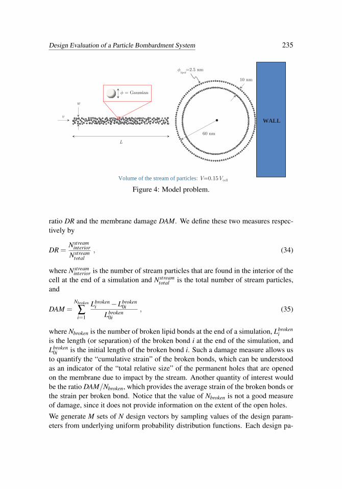
To perform the parametric simulations we are concerned with in this work, we de-vise the model problem that is depicted in Fig. 4. Accordingly, we consider thebombardment of a prokaryotic cell of an ideally circular shape. The cell has ex-ternal radius Rcell = 60 nm, membrane thickness of 10 nm and its lipid moleculeshave diameter φlipid = 2.5 nm. The stream is consisted of particles that occupya rectangular region of length L and width w, the area of which is constrained tobe 15% of the cell area (we say “area” but in a broader sense what we want toconstrain is the stream’s volume). Such a constraint is adopted to prevent large vol-umes of particles from being delivered to the interior of the cell, which could causeexcessive swelling and eventually cell rupture. The stream particles are consistedof a polymeric material and their diameters follow a Gaussian distribution of meanφmean and standard deviation σφ = 0.1φmean. Their travelling velocity when leavingthe tip of the gun is v. In our computational model, these particles are randomlyplaced within the region L×w by means of a standard random sequence additionalgorithm, with a packing ratio of 50% (for details on this and other types of par-ticle packing algorithms, the interested reader is referred to [Zhang and Torquato(2013)], and references therein).

For the analysis of different scenarios of delivery success and membrane damageupon bombardment of the cell, we consider the design parameters of the deliverysystem to be φmean, v and w (with L being constrained by L = 0.15πR2

cell/w). Thisleads to a parameter space that can be represented by a design vector ΛΛΛ as indicatedbelow:

ΛΛΛ = {φmean,v,w} . (33)

The indicators of performance for each design vector (i.e. measures that indicatewhether a design ΛΛΛ performs favorably or unfavorably) are taken as the delivery


w

10 nm

lipid

=2.5 nm

= Gaussian

L

60 nm

v

WALL

Volume of the stream of particles: V=0.15Vcell

Figure 4: Model problem.

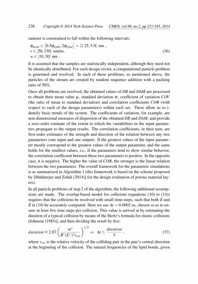
ratio DR and the membrane damage DAM. We define these two measures respec-tively by

DR =Nstream

interiorNstream

total, (34)

where Nstreaminterior is the number of stream particles that are found in the interior of the

cell at the end of a simulation and Nstreamtotal is the total number of stream particles,

and

DAM =Nbroken

∑i=1

Lbrokeni −Lbroken

0i

Lbroken0i

, (35)

where Nbroken is the number of broken lipid bonds at the end of a simulation, Lbrokeni

is the length (or separation) of the broken bond i at the end of the simulation, andLbroken

0i is the initial length of the broken bond i. Such a damage measure allows usto quantify the “cumulative strain” of the broken bonds, which can be understoodas an indicator of the “total relative size” of the permanent holes that are openedon the membrane due to impact by the stream. Another quantity of interest wouldbe the ratio DAM/Nbroken, which provides the average strain of the broken bonds orthe strain per broken bond. Notice that the value of Nbroken is not a good measureof damage, since it does not provide information on the extent of the open holes.

We generate M sets of N design vectors by sampling values of the design param-eters from underlying uniform probability distribution functions. Each design pa-


rameter is constrained to fall within the following intervals:

φmean ∈[0.5φlipid ,2φlipid

]= [1.25,5.0] nm ,

v ∈ [50,150] nm/ns ,w ∈ [10,30] nm .

(36)

It is assumed that the samples are statistically independent, although they need notbe identically distributed. For each design vector, a computational particle problemis generated and resolved. In each of these problems, as mentioned above, theparticles of the stream are created by random sequence addition with a packingratio of 50%.

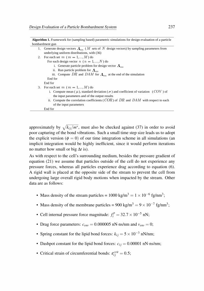
Once all problems are resolved, the obtained values of DR and DAM are processedto obtain their mean value µ , standard deviation σ , coefficient of variation COV(the ratio of mean to standard deviation) and correlation coefficients COR (withrespect to each of the design parameters) within each set. These allow us to i-dentify basic trends of the system. The coefficients of variation, for example, arenon-dimensional measures of dispersion of the obtained DR and DAM, and providea zero-order estimate of the extent to which the variabilities in the input parame-ters propagate to the output results. The correlation coefficients, in their turn, arefirst-order estimates of the strength and direction of the relation between any twoparameters (one input and one output). If the greatest values of the input parame-ter mostly correspond to the greatest values of the output parameter, and the sameholds for the smallest values, i.e., if the parameters tend to show similar behavior,the correlation coefficient between these two parameters is positive. In the oppositecase, it is negative. The higher the value of COR, the stronger is the linear relationbetween the two parameters. The overall framework for the parametric simulationsis as summarized in Algorithm 1 (this framework is based on the scheme proposedby [Mukherjee and Zohdi (2014)] for the design evaluation of porous material lay-ers).

In all particle problems of step 2 of the algorithm, the following additional assump-tions are made. The overlap-based model for collisions (equations (10) to (14))requires that the collisions be resolved with small time-steps, such that both δ andδ̇ in (10) be accurately computed. Here we use ∆t = 0.0002 ns, chosen so as to en-sure at least five time steps per collision. This value is arrived at by estimating theduration of a typical collision by means of the Hertz’s formula for elastic collisions[Johnson (1985)], and then dividing the result by five:

duration∼= 2.87(

m∗

R∗(E∗)2vrel

)1/5

⇒ ∆t ≤ duration5

, (37)

where vrel is the relative velocity of the colliding pair in the pair’s central directionat the beginning of the collision. The natural frequencies of the lipid bonds, given


Algorithm 1. Framework for (sampling based) parametric simulations for design evaluation of a particle

bombardment gun

1. Generate design vectors mn (M sets of N design vectors) by sampling parameters from

underlying uniform distributions, with (36)

2. For each set m ( 1,...,m M ) do

For each design vector n ( 1,...,n N ) do

i. Generate particle problem for design vector mn

ii. Run particle problem for mn

iii. Compute DR and DAM for mn at the end of the simulation

End for

End for

3. For each set m ( 1,...,m M ) do

i. Compute mean ( ), standard deviation ( ) and coefficient of variation (COV ) of

the input parameters and of the output results

ii. Compute the correlation coefficients (COR ) of DR and DAM with respect to each

of the input parameters

End for

approximately by√

ki j/m∗, must also be checked against (37) in order to avoidpoor capturing of the bond vibrations. Such a small time step size leads us to adoptthe explicit version (φ = 0) of our time integration scheme in all simulations (animplicit integration would be highly inefficient, since it would perform iterationsno matter how small or big ∆t is).

As with respect to the cell’s surrounding medium, besides the pressure gradient ofequation (21) we assume that particles outside of the cell do not experience anypressure forces, whereas all particles experience drag according to equation (6).A rigid wall is placed at the opposite side of the stream to prevent the cell fromundergoing large overall rigid body motions when impacted by the stream. Otherdata are as follows:

• Mass density of the stream particles = 1000 kg/m3 = 1×10−6 fg/nm3;

• Mass density of the membrane particles = 900 kg/m3 = 9×10−7 fg/nm3;

• Cell internal pressure force magnitude: f pi = 32.7×10−5 nN;

• Drag force parameters: cenv = 0.000005 nN·ns/nm and venv = 0;

• Spring constant for the lipid bond forces: ki j = 5×10−3 nN/nm;

• Dashpot constant for the lipid bond forces: ci j = 0.00001 nN·ns/nm;

• Critical strain of circumferential bonds: εcriti j = 0.5;


• Critical strain of radial and cross-wise bonds: εcriti j = 0.1;

• Elasticity modulus of stream and membrane particles (needed to resolve col-lisions): E jet = Elipid = 100 nN/nm2;

• Poisson coefficient of stream and membrane particles (needed to resolve col-lisions): ν jet = νlipid = 0.25;

• Damping rate for particle-particle collisions: ξ = 0.1;

• Coefficient of dynamic friction for particle-particle collisions: µd = 0.1;

• Gravity is neglected (ggg = o);

• Initial distance between stream front and cell exterior = 10 nm;

• Rigid wall properties: µd = 0.1 and ξ = 0.1;

• Time step size = 0.0002 ns;

• Final time at the end of each simulation = 10 ns.

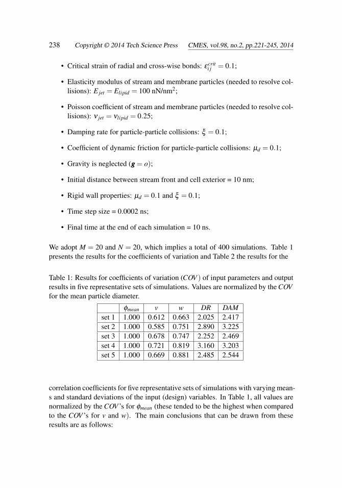
We adopt M = 20 and N = 20, which implies a total of 400 simulations. Table 1presents the results for the coefficients of variation and Table 2 the results for the

Table 1: Results for coefficients of variation (COV ) of input parameters and outputresults in five representative sets of simulations. Values are normalized by the COVfor the mean particle diameter.

φmean v w DR DAMset 1 1.000 0.612 0.663 2.025 2.417set 2 1.000 0.585 0.751 2.890 3.225set 3 1.000 0.678 0.747 2.252 2.469set 4 1.000 0.721 0.819 3.160 3.203set 5 1.000 0.669 0.881 2.485 2.544

correlation coefficients for five representative sets of simulations with varying mean-s and standard deviations of the input (design) variables. In Table 1, all values arenormalized by the COV ’s for φmean (these tended to be the highest when comparedto the COV ’s for v and w). The main conclusions that can be drawn from theseresults are as follows:


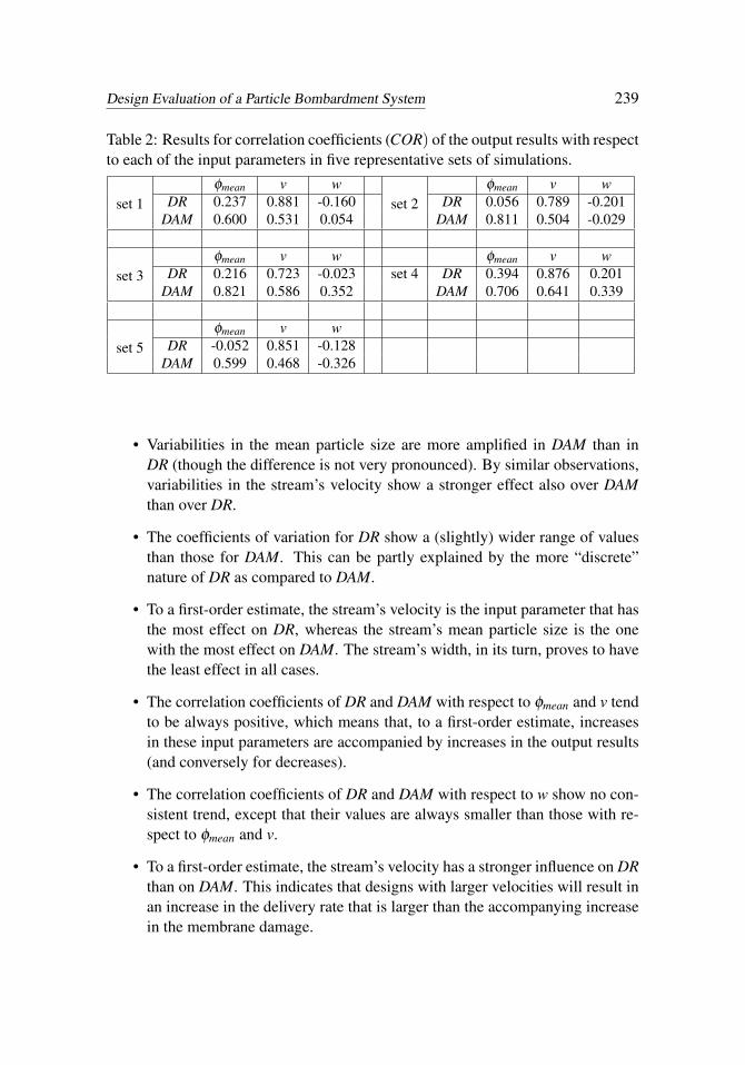
Table 2: Results for correlation coefficients (COR) of the output results with respectto each of the input parameters in five representative sets of simulations.

set 1φmean v w

set 2φmean v w

DR 0.237 0.881 -0.160 DR 0.056 0.789 -0.201DAM 0.600 0.531 0.054 DAM 0.811 0.504 -0.029

set 3φmean v w φmean v w

DR 0.216 0.723 -0.023 set 4 DR 0.394 0.876 0.201DAM 0.821 0.586 0.352 DAM 0.706 0.641 0.339

set 5φmean v w

DR -0.052 0.851 -0.128DAM 0.599 0.468 -0.326

• Variabilities in the mean particle size are more amplified in DAM than inDR (though the difference is not very pronounced). By similar observations,variabilities in the stream’s velocity show a stronger effect also over DAMthan over DR.

• The coefficients of variation for DR show a (slightly) wider range of valuesthan those for DAM. This can be partly explained by the more “discrete”nature of DR as compared to DAM.

• To a first-order estimate, the stream’s velocity is the input parameter that hasthe most effect on DR, whereas the stream’s mean particle size is the onewith the most effect on DAM. The stream’s width, in its turn, proves to havethe least effect in all cases.

• The correlation coefficients of DR and DAM with respect to φmean and v tendto be always positive, which means that, to a first-order estimate, increasesin these input parameters are accompanied by increases in the output results(and conversely for decreases).

• The correlation coefficients of DR and DAM with respect to w show no con-sistent trend, except that their values are always smaller than those with re-spect to φmean and v.

• To a first-order estimate, the stream’s velocity has a stronger influence on DRthan on DAM. This indicates that designs with larger velocities will result inan increase in the delivery rate that is larger than the accompanying increasein the membrane damage.


• To a first-order estimate, the stream’s mean particle size has a remarkablystronger influence on DAM than on DR. This indicates that designs withlarger particles will result in an increase in the membrane damage that ismuch larger than the accompanying increase in the delivery rate.

0

20

40

60

80

100

120

140

160

0.0 1.0 2.0 3.0 4.0 5.0 6.0

Mean diameter versusDAM

0

20

40

60

80

100

120

140

160

0 50 100 150 200

Velocity versusDAM

0

5

10

15

20

25

30

35

0.0 1.0 2.0 3.0 4.0 5.0 6.0

Mean diameter versusDR

0

5

10

15

20

25

30

35

0 50 100 150 200

Velocity versusDR

DR

(%

)

DA

M

DR

(%

) Mean particle diameter (nm) Mean particle diameter (nm)

DA

M

Stream velocity (nm/ns) Stream velocity (nm/ns)

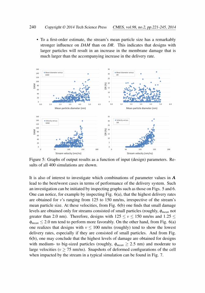
Figure 5: Graphs of output results as a function of input (design) parameters. Re-sults of all 400 simulations are shown.

It is also of interest to investigate which combinations of parameter values in ΛΛΛ

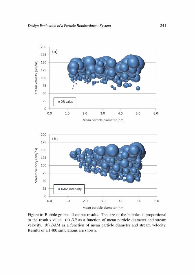
lead to the best/worst cases in terms of performance of the delivery system. Suchan investigation can be initiated by inspecting graphs such as those on Figs. 5 and 6.One can notice, for example by inspecting Fig. 6(a), that the highest delivery ratesare obtained for v’s ranging from 125 to 150 nm/ns, irrespective of the stream’smean particle size. At these velocities, from Fig. 6(b) one finds that small damagelevels are obtained only for streams consisted of small particles (roughly, φmean notgreater than 2.0 nm). Therefore, designs with 125 ≤ v ≤ 150 nm/ns and 1.25 ≤φmean ≤ 2.0 nm tend to perform more favorably. On the other hand, from Fig. 6(a)one realizes that designs with v ≤ 100 nm/ns (roughly) tend to show the lowestdelivery rates, especially if they are consisted of small particles. And from Fig.6(b), one may conclude that the highest levels of damage are obtained for designswith medium- to big-sized particles (roughly, φmean ≥ 2.5 nm) and moderate tolarge velocities (v ≥ 75 nm/ns). Snapshots of deformed configurations of the cellwhen impacted by the stream in a typical simulation can be found in Fig. 7.


0

25

50

75

100

125

150

175

200

0.0 1.0 2.0 3.0 4.0 5.0 6.0

DR value

Mean particle diameter (nm)

Stre

am v

elo

city

(n

m/n

s)

(a)

0

25

50

75

100

125

150

175

200

0.0 1.0 2.0 3.0 4.0 5.0 6.0

DAM intensity

Mean particle diameter (nm)

Stre

am v

elo

city

(n

m/n

s)

(b)

Figure 6: Bubble graphs of output results. The size of the bubbles is proportionalto the result’s value. (a) DR as a function of mean particle diameter and streamvelocity. (b) DAM as a function of mean particle diameter and stream velocity.Results of all 400 simulations are shown.


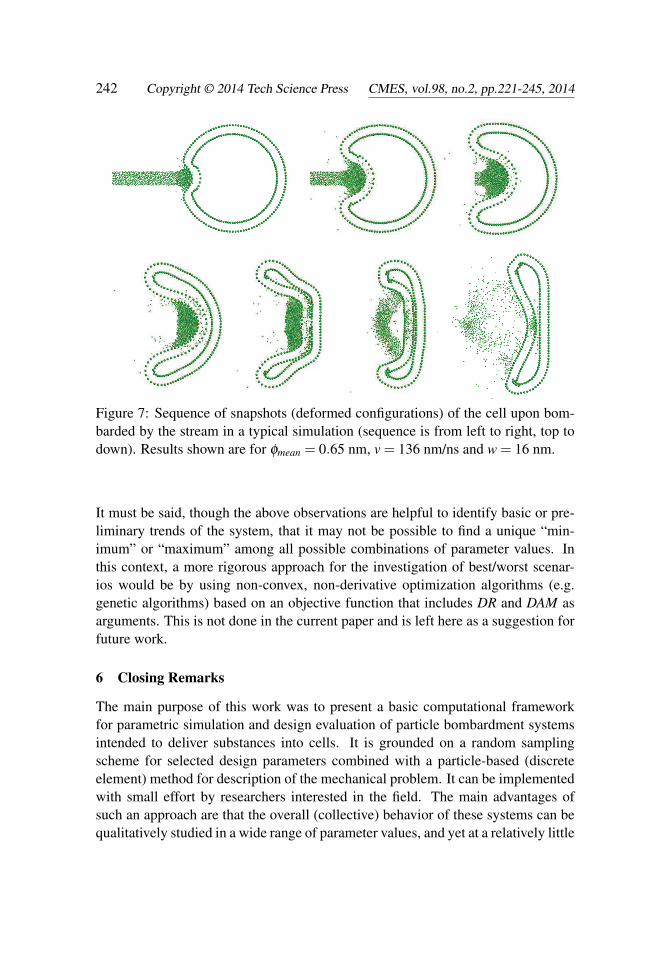
Figure 7: Sequence of snapshots (deformed configurations) of the cell upon bom-barded by the stream in a typical simulation (sequence is from left to right, top todown). Results shown are for φmean = 0.65 nm, v = 136 nm/ns and w = 16 nm.

It must be said, though the above observations are helpful to identify basic or pre-liminary trends of the system, that it may not be possible to find a unique “min-imum” or “maximum” among all possible combinations of parameter values. Inthis context, a more rigorous approach for the investigation of best/worst scenar-ios would be by using non-convex, non-derivative optimization algorithms (e.g.genetic algorithms) based on an objective function that includes DR and DAM asarguments. This is not done in the current paper and is left here as a suggestion forfuture work.

6 Closing Remarks

The main purpose of this work was to present a basic computational frameworkfor parametric simulation and design evaluation of particle bombardment systemsintended to deliver substances into cells. It is grounded on a random samplingscheme for selected design parameters combined with a particle-based (discreteelement) method for description of the mechanical problem. It can be implementedwith small effort by researchers interested in the field. The main advantages ofsuch an approach are that the overall (collective) behavior of these systems can bequalitatively studied in a wide range of parameter values, and yet at a relatively little


computational cost. It allows for the identification of basic trends of the systemupon changes on the design parameters, and offers a good picture for investigationof best/worst case scenarios.

We remark that our intention here was simply to show how the framework worksfrom a general perspective. To this end, we have selected as design parameters onlythe stream’s mean particle size, width and incoming velocity. Of course, the influ-ence of other parameters could have been studied as well, such as the cell’s internalpressure, bonding stiffnesses, friction coefficients, etc. These quantities could havealso been treated as random variables and have the effects of the variabilities oftheir values assessed.

Kernel density estimation techniques (e.g. with a Gaussian kernel) can be usedto construct the probability distribution functions of both DR and DAM. This canbe straightforwardly done from the mean values of these output parameters in ran-domly selected sets of simulations. From the generated distributions, probabilitiesof excellence of specified thresholds of DR and DAM (e.g. the probability that thevalue of DAM is higher than a given value) can be obtained. This can be very usefulinformation. Also, based on these distributions one may define an index of success(or, equivalently, an index of failure) to quantify how well a cell will respond uponimpact by a stream of particles with given design parameters (or, in other words,how well a delivery system with given design parameters will succeed in deliveringsubstances to the interior of a cell).

Particle-based computational models allow for the construction of rapid simulationtools. We believe they are a very useful approach for design evaluation of deliverymechanisms, lessening the number of (costly and delicate) physical experimentsand thus helping advance the design of particle-gun delivery systems.

Acknowledgement: This work was supported by FAPESP (Fundação de Am-paro à Pesquisa do Estado de São Paulo), under the grant 2012/04009-0 (whichmade possible a research stay for the first author at the University of Californiaat Berkeley, on a sabbatical leave from the University of São Paulo), and by CNPq(Conselho Nacional de Desenvolvimento Científico e Tecnológico), under the grant303793/2012-0. Material support and the stimulating discussions in CMRL (Com-putational Materials Research Laboratory, Department of Mechanical Engineering,UC Berkeley) are also gratefully acknowledged.

References

Andoh, Y.; Okazaki, S.; Ueoka, R. (2013): Molecular dynamics study of lipid bi-layers modeling the plasma membranes of normal murine thymocytes and leukemic


GRSL cells. Biochim Biophys Acta, vol. 1828, no. 4, pp. 1259-1270.

Axelsson, A. (1994): Iterative solution methods. Cambridge Univeristy Press.

Bicanic, N. (2004): Discrete Element Methods. Encyclopedia of ComputationalMechanics, Volume 1: Fundamentals. Stein E, de Borst R, Hughes TJR (eds).John Wiley & Sons.

Campello, E. M. B; Zohdi, T. I. (2014): A computational framework for simula-tion of the delivery of substances into cells (DOI: 10.1002/cnm.2649). Internation-al Journal for Numerical Methods in Biomedical Engineering.

Campello, E. M. B. (2014): Computational modeling and simulation of ruptureof membranes and thin films (accepted for publication). Journal of the BrazilianSociety of Mechanical Sciences and Engineering.

Cundall, P. A.; Strack, O. D. L. (1979): A discrete numerical model for granularassemblies. Geotech, vol. 29, pp. 47–65.

Delemotte, L.; Tarek, M. (2012): Molecular dynamics simulations of lipid mem-brane electroporation. J Membr Biol, vol. 245, no. 9, pp. 531-543.

Duran, J. (1997): Sands, Powders and Grains: An introduction to the physics ofgranular matter. Springer.

Hac, A. E.; Seeger, H. M.; Fidorra, M.; Heimburg, T. (2005): Diffusion inTwo-Component Lipid Membranes –A Fluorescence Correlation Spectroscopy andMonte Carlo Simulation Study. Biophys J, vol. 88, pp. 317-333.

Israelachvili, J. N. (2011): Intermolecular and surface forces. Elsevier.

Johnson, K. L.; Kendall, K.; Roberts, A. D. (1971): Surface energy and thecontact of elastic solids. Proc R Soc Lond A, vol. 324, pp. 301–313.

Johnson, K. L. (1985): Contact Mechanics. Cambridge University Press.

Khelashvili, G.; Weinstein, H.; Harries, D. (2008): Protein diffusion on chargedmembranes: A dynamic mean-field model describes time evolution and lipid reor-ganization. Biophys J, vol. 94, pp. 2580-2597.

Klein, T. M.; Wolf, E. D.; Wu, R.; Sanford, J. C. (1987): High-velocity micro-projectiles for delivering of nucleic acids into living cells. Nature, vol. 327, pp.70-73.

Lennard-Jones, J. E. (1924): On the Determination of Molecular Fields. Proc. R.Soc. Lond. A, vol. 106, no. 738, pp. 463–477.

Mukherjee, D.; Zohdi, T. I. (2014): Rapid parametric simulations for design e-valuation and uncertainty characterization of a porous material layer impacted by aparticle (accepted for publication). International Journal of Impact Engineering.

Pastor, R. W.; Venable, R. M. (1993): Molecular and stochastic dynamics sim-


ulations of lipid membranes. In: van Gunsteren WF, Weiner PK, Wilkinson AK(Eds.). Computer Simulation of Biomolecular Systems: Theoretical and Experi-mental Applications, Chap. 2, pp. 443-464. Escom Science Publishers.

Pastor, R.W. (1994): Molecular dynamics and Monte Carlo simulations of lipidbilayers. Curr Opin Struct Biol, vol. 4, pp. 486–492.

Pöschel, T.; Schwager, T. (2004): Computational Granular Dynamics. Springer.

Rangamani, P.; Agrawal, A.; Mandadapu, K. K.; Oster, G.; Steigmann, D.(2013): Interaction between surface shape and intra-surface viscous flow on lipidmembranes. Biomech Model Mechanobiol, vol. 12, pp. 833-845.

Sanford, J. C.; Klein, T. M.; Wolf, E. D.; Allen, N. (1987): Delivery of substancesinto cells and tissues using a particle bombardment process. Particulate Scienceand Technology: An International Journal, vol. 5, pp. 27-37.

Tieleman, D. P.; Marrink, S. J.; Berendsen, H. J. C. (1997): Computer perspec-tive of membranes: molecular dynamics studies of lipid bilayer systems. BiochimBiophys Acta, vol. 1331, pp. 235–270.

Wang, Y.; Sigurdsson, J. K.; Brandt, E.; Atzberger, P. J. (2013): Dynamicimplicit-solvent coarse-grained models of lipid bilayer membranes: Fluctuating hy-drodynamics thermostat. Phys Rev E, vol. 88, pp. 023301-1-5.

Wellmann, C.; Wriggers, P. (2012): A two-scale model of granular materials.Comput Methods Appl Mech Engrg, vol. 205–208, pp. 46–58.

Zhang, G.; Torquato, S. (2013): Precise algorithm to generate random sequentialaddition of hard hyperspheres at saturation. Phys Rev E, vol. 88, pp. 053312-1-9.

Zohdi, T. I. (2012): Dynamics of charged particulate systems: Modeling, theoryand computation. Springer.

Design Evaluation of a Particle Bombardment System Used to ...

Documents

Transcript of Design Evaluation of a Particle Bombardment System Used to ...