
Design, Construction and Load Testing of the Bridge on ...
54
Design, Construction and Load Testing of the Bridge on Arnault Branch, Washington County, Missouri Using Innovative Technologies by Sahra Sedigh Sarvestani, Ph.D. at Missouri University of Science and Technology Dongming Yan, Ph.D. Genda Chen, Ph.D., P.E. Nestore Galati, Ph.D., P.E. A University Transportation Center Program UTC R193
Transcript of Design, Construction and Load Testing of the Bridge on ...

Design, Construction and Load Testing of the Bridge on Arnault Branch,
Washington County, Missouri Using Innovative Technologies
by
Sahra Sedigh Sarvestani, Ph.D.
at Missouri University of Science and Technology
Dongming Yan, Ph.D.
Genda Chen, Ph.D., P.E. Nestore Galati, Ph.D., P.E.
A University Transportation Center Program
UTC R193

Disclaimer
The contents of this report reflect the views of the author(s), who are responsible for the facts and the
accuracy of information presented herein. This document is disseminated under the sponsorship of
the Department of Transportation, University Transportation Centers Program and the Center for
Infrastructure Engineering Studies UTC program at the Missouri University of Science and
Technology, in the interest of information exchange. The U.S. Government and Center for
Infrastructure Engineering Studies assumes no liability for the contents or use thereof.
NUTC ###

Technical R age
2. Government Accession No. Recipient's Catalog No. eport Documentation P
1. Report No.
UTC R193
3.
5. Report Date
February 2010
4. Title and Subtitle Design, Construction and Load Testing of the Bridge on Arnault Branch, Washington County, Missouri Using Innovative Technologies
6. Performing Organization Code 7. Author/s
Dongming Yan, Ph.D., Genda Chen, Ph.D., P.E., Nestore Galati, Ph.D., P.E. and Sahra Sedigh
rganization Report No.
00016277 Sarvestani, Ph.D.
8. Performing O
10. Work Unit No. (TRAIS) 9. Performing Organization Name and Address
Center for Infrastructure Engineering Studies/UTMissouri University of Science a220 Engineering R
C program nd Technology
esearch Lab
o.
DTRS98-G-0021
Rolla, MO 65409
11. Contract or Grant N
13. Type of Report and Period Covered
Final
12. Sponsoring Organization Name and Address
U.S. Department of Transportation Research and Innovative Techn1200 New Jersey Avenue
ology Administration , SE
14. Sponsoring Agency Code
Washington, DC 20590
15. Supplementary Notes
16.
er the completion of bridge construction. The collected l allow the study of FRP bars and stay-in-place
Abstract The superstructure and instrumentation designs of a three-span bridge are presented in this report. The three spans include a precast box-girder bridge, a precast deck on steel girder and a precast deck on concrete girder. They were designed to compare the performance of various bridge decks reinforced with fiber reinforced polymers (FRP) through field instrumentations. A wireless monitoring system was designed to facilitate the collection of field data aftdata wil FRP grid systems.
17. Key Words
Bridge design, concrete deck, GFRP bars, Service, Spr nia 2and bridge instrumentation
18. Distribution Statement
No restrictions. This document is available to the public through the National Technical Information ingfield, Virgi 2161.
19. Security Classification (of this report)
unclassified
ication (of this page) 21. No. O ges
50
22. Price 20. Security Classif
unclassified
f Pa
Form DOT F 1700.7 (8-72)

ii
The mission of CIES is to provide leadership in research and education for solving society's problems affecting the nation's infrastructure systems. CIES is the primary conduit for communication among those on the MST campus interested in infrastructure studies and provides coordination for collaborative efforts. CIES activities include interdisciplinary research and development with projects tailored to address needs of federal agencies, state agencies, and private industry as well as technology transfer and continuing/distance education to the engineering community and industry.
Center for Infrastructure Engineering Studies (CIES) Missouri University of Science and Technology
223 Engineering Research Laboratory 1870 Miner Circle
Rolla, MO 65409-0710 Tel: (573) 341-4497; fax -6215
E-mail: [email protected] http://www.cies.mst.edu/

iii
RESEARCH INVESTIGATION
Design, Construction and Load Testing of the Bridge on Arnault Branch,
Washington County, Missouri Using Innovative Technologies
PREPARED FOR THE
GREAT RIVER ENGINEERING
IN COOPERATION WITH THE
CENTER FOR TRANSPORTATION INFRASTRUCTURE AND SAFETY
Written by:
Dongming Yan, Ph.D.
Genda Chen, Ph.D., P.E.
Nestore Galati, Ph.D., P.E.
Sahra Sedigh Sarvestani, Ph.D.
CENTER FOR INFRASTRUCTURE ENGINEERING STUDIES
MISSOURI UNIVERSITY OF SCIENCE AND TECHNOLOGY
Submitted January 10, 2010
The opinions, findings and conclusions expressed in this report are those of the principal investigators. They are not necessarily those of the Missouri Department of Transportation, U.S. Department of Transportation, Federal Highway Administration. This report does not constitute
a standard, specification or regulation.

iv
TABLE OF CONTENTS
LIST OF FIGURES ....................................................................................................................... vi
LIST OF TABLES........................................................................................................................ vii
NOTATIONS............................................................................................................................... viii
1 INTRODUCTION .....................................................................................................................1 1.1 Background and Significance of Work............................................................................1 1.2 Objectives of the Overall Project.....................................................................................2 1.3 Report Outline..................................................................................................................3
2 BRIDGE STRUCTURAL ANALYSIS.....................................................................................4 2.1 Precast GFRP-Reinforced Concrete Box Girders............................................................4
2.1.1 General layout of hollow slabs ....................................................................................4 2.1.2 Slab analysis.................................................................................................................5
2.1.2.1 Material properties.......................................................................................................... 5 2.1.2.2 Dead load........................................................................................................................ 5 2.1.2.3 Live load: truck and tandem ......................................................................................... 6 2.1.2.4 Live load: design lane load............................................................................................. 7 2.1.2.5 Load combination........................................................................................................... 7 2.1.2.6 Flexural moment capacity: ............................................................................................. 9 2.1.2.7 Cracking evaluation...................................................................................................... 10 2.1.2.8 Deflection ..................................................................................................................... 11
2.1.3 Shear design ...............................................................................................................13 2.1.3.1 Shear strength ............................................................................................................... 13
2.1.4 Development length ...................................................................................................14 2.2 Precast GFRP-Reinforced Panels on Steel Girders .......................................................15
2.2.1 AASHTO deck design ...............................................................................................15 2.2.2 Deck analysis .............................................................................................................17
2.2.2.1 Live load effects ........................................................................................................... 18 2.2.2.2 Positive moment analysis ............................................................................................. 19 2.2.2.3 Design negative moment at interior girders ................................................................. 21
2.2.3 Cantilever analysis .....................................................................................................22 2.2.4 Girder design..............................................................................................................23
2.3 Precast GFRP-Reinforced Concrete Panels on Concrete Girders..................................24 2.3.1 Preliminary deck design according to CSA code ......................................................24 2.3.2 Deck analysis with AASHTO specifications.............................................................26
2.3.2.1 Positive moment analysis ............................................................................................. 26 2.3.2.2 Design negative moment at interior girders ................................................................. 30 2.3.2.3 Cantilever analysis........................................................................................................ 30
2.3.3 Deck analysis with CSA code....................................................................................30 2.3.3.1 Design for deformability .............................................................................................. 30 2.3.3.2 Minimum flexural resistance ........................................................................................ 31 2.3.3.3 Crack-control reinforcement......................................................................................... 31

v
2.3.3.4 Non-prestressed reinforcement..................................................................................... 31 2.3.4 Girder analysis with AASHTO specifications...........................................................32
3 BRIDGE INSTRUMENTATION ...........................................................................................34 3.1 Design of the Structural Health Monitoring Platform ...................................................34 3.2 Evaluation Results .........................................................................................................37
3.2.1 Test 1: Direct connection of coordinator and end device ..........................................38 3.2.2 Test 2: Indirect connection of coordinator and end device........................................38 3.2.3 Test 3: Direct connection of coordinator and end device (Burst Mode)....................38
3.3 Planned Instrumentation Layout ....................................................................................39 4 CONCLUDING REMARKS...................................................................................................40
REFERENCES ..............................................................................................................................41
APPENDIX: MORE DATA RELATED TO THE SPAN WITH STEEL GIRDERS..................42

vi
LIST OF FIGURES Figure 1 Overall plan view ............................................................................................................ 2
Figure 2 Bridge design plan............................................................................................................ i
Figure 3 Elevation view of the box-girder span............................................................................. 4
Figure 4 Cross section of a box girder or a hollow slab ................................................................. 4
Figure 5 Reinforcement distribution............................................................................................... 5
Figure 6 Cross section of a box girder ............................................................................................ 6
Figure 7 Design Truck ................................................................................................................... 6
Figure 8 Positions of various loads applied on the simply-supported box girder.......................... 8
Figure 9 Dimensions of a box-girder cross section ........................................................................ 9
Figure 10 Elevation view of the bridge......................................................................................... 15
Figure 11 Bridge deck designed according to AASHTO Specifications...................................... 16
Figure 12 Cantilever loading diagram ......................................................................................... 22
Figure 13 Cross sectional view of the deck with inverted T-girders ............................................ 24
Figure 14 Recommended cross-section of inverted T-girder ....................................................... 24
Figure 15 Plan view of the deck with concrete inverted T-girders............................................... 26
Figure 16 Block diagram of the SmartBrick structural health monitoring network ..................... 35
Figure 17 Snapshot of data visualization provided through web interface................................... 36
Figure 18 One of two test configurations ..................................................................................... 37
Figure 19 Instrumentation layout.................................................................................................. 39
Figure 20 Leveling and grout pocket details................................................................................. 42

vii
LIST OF TABLES
Table 1 Guaranteed tensile properties...................................................................................... 5
Table 2 GFRP reinforcement size, spacing and ratio............................................................. 16
Table 3 Negative moments (k-ft/ft) ....................................................................................... 18
Table 4 Reinforcement size, spacing and ratios..................................................................... 25
Table 5 Open-air test results .................................................................................................. 38

viii
NOTATIONS
A = The effective tension area of concrete, defined as the area of concrete having the same centroid as that of tensile reinforcement, divided by the number of bars
A1 = Factor for dead loads
A2 = Factor for live loads
fA = Area of FRP reinforcement
fpA = Area of post-tensioned FRP reinforcement
,f tsA = Area of shrinkage and temperature FRP reinforcement
sA = Area of steel reinforcement
b = Web width
c = Distance from extreme compression fiber to the neutral axis
C = Capacity
CE = Environmental reduction factor
d = Distance from extreme compression fiber to centroid of tension reinforcement
dc = Thickness of the concrete cover measured from extreme tension fiber to the center of the bar
pd = Distance from extreme compression fiber to centroid of prestressed reinforcement
D = Dead load
E = Width of the slab
Ec = Modulus of elasticity of concrete
Ef = Guaranteed modulus of elasticity of FRP
Ep = Modulus of elasticity of CFRP
Es = Guaranteed modulus of elasticity of steel
Esl = Modulus of elasticity of the concrete of the slab '
cf = Specified compressive strength of concrete
ff = Stress at service in the FRP
fuf = Design tensile strength of FRP, considering reductions for service environment
*fuf = Guaranteed tensile strength of an FRP bar
fupf = Design tensile strength of post-tensioned FRP

ix
I = Live load impact
Isl = Moment of inertia of the slab cross section
kb = Bond-dependant coefficient
l = Slab length
L = Live load
M = Flexural moment
DLM = Moment due to the dead load
LLM = Moment due to the live load
maxM − = Maximum negative flexural moment acting on the specimen
maxM +
= Maximum positive flexural moment acting on the specimen
Mn = Nominal flexural capacity of an FRP reinforced concrete member
Mpi = Bending moment to the centroid of the section induced by the post-tensioning of the CFRP
bars
sM = Service moment per unit strip of slab deck
uM = Factored moment at section
N = Number of bars
P = Concentrated force
S = Length of the slab
cV = Nominal shear strength provided by concrete with steel flexural reinforcement
,c fV = Nominal shear strength provided by concrete with FRP flexural reinforcement
maxV − = Maximum negative shear acting on the specimen
maxV − = Maximum positive shear acting on the specimen
Vn = Nominal shear strength at section
uV = Factored shear force at section
w = Crack width
W = Weight of the nominal truck
LLω = Impact factor

x
β = Ratio of the distance from the neutral axis to extreme tension fiber to the distance from the
neutral axis to the center of tensile reinforcement
1β = Factor depending on the concrete strength
βd = Coefficient given by AASHTO
cε = Strain in concrete
fε = Strain in FRP reinforcement
fuε = Design rupture strain of FRP reinforcement
*fuε = Guaranteed rupture strain of FRP reinforcement
pε = Strain in prestressed CFRP
Δ = Long term deflection
LLΔ = Deflection due to the live load
DLΔ = Deflection due to the dead load
φ = Strength reduction factor
λ = Multiplier for additional long-term deflection
fρ = FRP reinforcement ratio
fbρ = FRP reinforcement ratio producing balanced strain conditions
,f tsρ = Reinforcement ratio for temperature and shrinkage FRP reinforcement

1
1 INTRODUCTION
This report describes the superstructure and instrumentation design of the bridge on Arnault Branch, Washington County, Missouri. Reinforced with fiber reinforced polymers (FRP) bars, the bridge deck is designed by a team consisting of the Center of Infrastructures Engineering Studies (CIES) at the Missouri University of Science and Technology (S&T), Great River Engineering (GRE), and Hughes Brothers. The bridge structure is designed using the load configuration and the analysis procedure specified in the 2007 AASHTO LRFD Design Specifications.
1.1 Background and Significance of Work
The overpass located on Pat Daly Road, over Arnault Branch (Washington County, MO) was in critical need of replacement with a more efficient bridge. The overpass was a 1.52 m (5 ft) thick unreinforced concrete slab-on-ground, with a total length of 12.19 m (40 ft) and width of 4.57 m (15 ft). The approach roadway was 4.88 m (16 ft) wide. Two 0.91 m (3 ft) diameter corrugated steel pipes run parallel through the concrete underneath the roadway and allowed water flowing. The slab-on-ground was structurally and functionally inadequate, and poses a safety threat. Specifically:
The overpass was frequently subjected to severe flood, due to a) insufficient distance between the roadway and the water level of the branch (1.52 m (5 ft)), and b) insufficient dimension of the through-concrete pipes to allow adequate water flowing. Floods result in disruption to traffic (requiring a 30 minute detour), as well as in gradually eroding the roadway pavement, that is in need of continuous maintenance.
The use of unreinforced concrete as the sole overpass building material, combined with the significant amount of heavy vehicles crossing the branch, has resulted in a fairly irregular and presumably unstable roadway. This required frequent inspections.
The width of the overpass, along with the deterioration of a significant portion of the roadway edges, did not allow the safe crossing of two vehicles at the same time. This resulted in numerous vehicular accidents during past years.
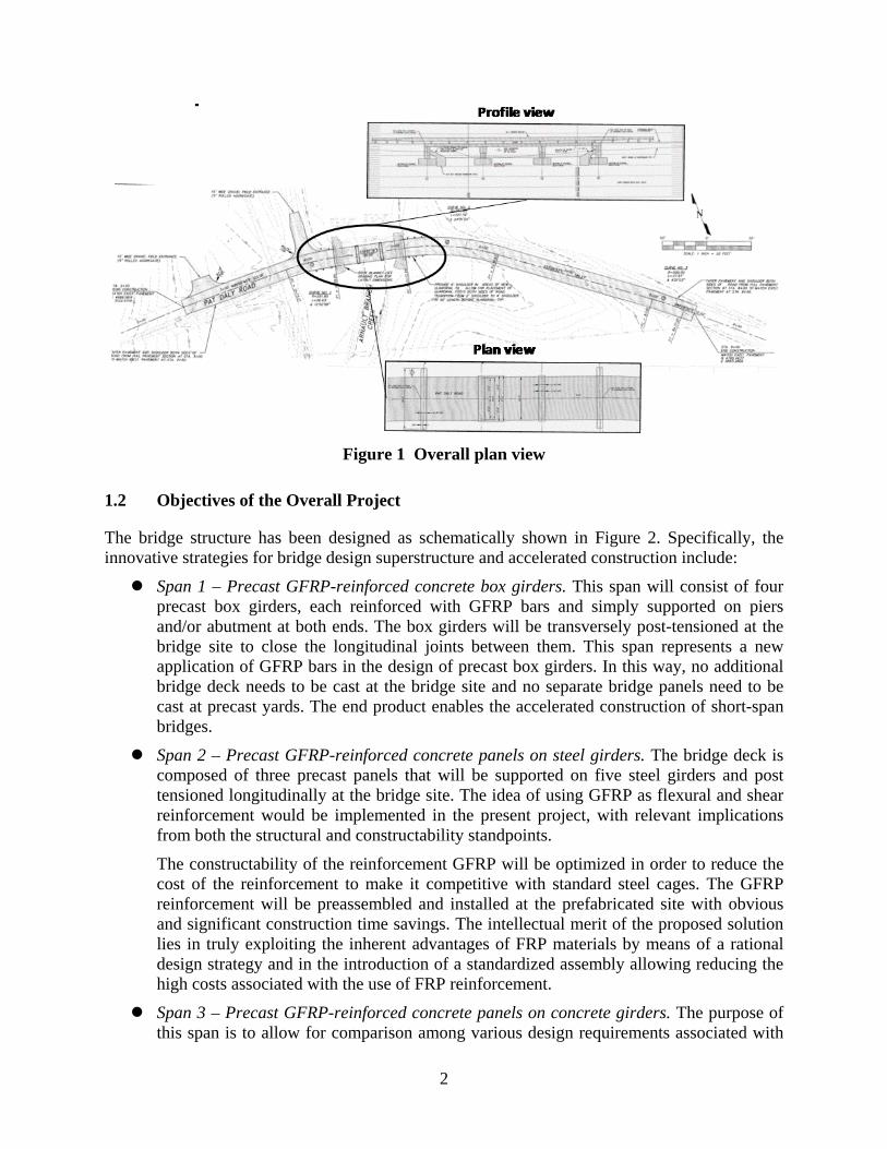
It was decided to replace the slab-on-ground overpass with a rapidly constructed glass fiber reinforced polymer (GFRP) reinforced concrete slab bridge as schematically shown in Figure 1. The new bridge will have three 8.23 m (27 ft) long simply-supported spans or a total length of 24.69 m (81 ft), and out-to-out deck width of 6.10 m (20 ft).
The increased length and clearance between roadway and water level will allow minimizing the risk of flood, while the increased roadway width will provide a functional mean to improve safety under normal traffic conditions.
2
Figure 1 Overall plan view
1.2 Objectives of the Overall Project
The bridge structure has been designed as schematically shown in Figure 2. Specifically, the innovative strategies for bridge design superstructure and accelerated construction include:
Span 1 – Precast GFRP-reinforced concrete box girders. This span will consist of four precast box girders, each reinforced with GFRP bars and simply supported on piers and/or abutment at both ends. The box girders will be transversely post-tensioned at the bridge site to close the longitudinal joints between them. This span represents a new application of GFRP bars in the design of precast box girders. In this way, no additional bridge deck needs to be cast at the bridge site and no separate bridge panels need to be cast at precast yards. The end product enables the accelerated construction of short-span bridges.
Span 2 – Precast GFRP-reinforced concrete panels on steel girders. The bridge deck is composed of three precast panels that will be supported on five steel girders and post tensioned longitudinally at the bridge site. The idea of using GFRP as flexural and shear reinforcement would be implemented in the present project, with relevant implications from both the structural and constructability standpoints.
The constructability of the reinforcement GFRP will be optimized in order to reduce the cost of the reinforcement to make it competitive with standard steel cages. The GFRP reinforcement will be preassembled and installed at the prefabricated site with obvious and significant construction time savings. The intellectual merit of the proposed solution lies in truly exploiting the inherent advantages of FRP materials by means of a rational design strategy and in the introduction of a standardized assembly allowing reducing the high costs associated with the use of FRP reinforcement.
Span 3 – Precast GFRP-reinforced concrete panels on concrete girders. The purpose of this span is to allow for comparison among various design requirements associated with

3
different types of girders and with different specifications.
Substructure. The substructure will be constructed using high grade MMFX steel. The current focus for MMFX’s core technology is uncoated steel that has a microstructure fundamentally different from conventional steel; in fact, this revolutionary technology has produced steel unlike any steel material ever introduced to the marketplace. Typical carbon steels form a matrix of chemically dissimilar materials – carbide and ferrite. These carbides are strong, yet brittle – immovable at the grain boundaries. In a moist environment, a battery-like effect occurs between the carbides and the ferrites that destroy the steel from the inside out. This effect (a microgalvanic cell) is the primary corrosion initiator that drives the corrosion reaction. MMFX steel has a completely different structure at the nano or atomic scale (a laminated lath structure resembling “plywood”). Steel made using MMFX nanotechnology does not form microgalvanic cells (the driving force behind corrosion). MMFX’s “plywood” effect lends good strength, ductility, toughness and corrosion resistance. The use of MMFX steel in the substructure will allow for a complete non-corrosive system for the bridge structure.
Figure 2 Bridge design plan
Instrumentation. The bridge will be instrumented with the SmartBrick platform, which is a wireless sensor network with long-range communication capability. Information pertinent to the structural health, e.g., strain, and surrounding environment, e.g, water level, of the bridge will be autonomously recorded and reported to a remote repository using the cellular phone network at regular intervals, on-demand, or as triggered by abnormal conditions.
1.3 Report Outline
This report consists of four main sections:
• Section 1 describes the project and introduces the objectives of the research. • Section 2 details the design calculations for the Washington County Bridge. • Section 3 describes instrumentation plans for the bridge. • Section 4 concludes this report.
Precast FRP-reinforced concrete panels supported on steel girders
Precast FRP-reinforced concrete panels on RC girders
Precast FRP-reinforced concrete box girders

4
2 BRIDGE STRUCTURAL ANALYSIS
2.1 Precast GFRP-Reinforced Concrete Box Girders
2.1.1 General layout of hollow slabs
The concrete box girder span consists of four precast, twin-cell hollow slabs that are transversely post tensioned at the bridge site to make longitudinal joints between girders always remain closed. The slabs are reinforced with Aslan 100 GFRP bars that are manufactured by Hughes Brothers. They were designed in accordance with the 2007 AASHTO LRFD Specifications and ACI 440 Specifications. Each slab was considered as a simply-supported beam for structural analysis, as shown in Error! Reference source not found.. The cross section and longitudinal reinforcement layout of each hollow slab are presented in Error! Reference source not found. and Error! Reference source not found., respectively.
Figure 3 Elevation view of the box-girder span
Figure 4 Cross section of a box girder or a hollow slab
6” o.c.

5
Figure 5 Reinforcement distribution
2.1.2 Slab analysis
2.1.2.1 Material properties
Internal FRP reinforcement was designed according to ACI 440 Guidelines (2006). Their initial material properties such as the ultimate tensile strength were used without considering the long-term exposure to environmental conditions. According to ACI 440, the design properties of FRP materials can generally be expressed into:
*
*
fu E fu
fu E fu
f C f
Cε ε
=
=
where ffu and εfu are the design tensile strength and the ultimate strain of FRP materials, and f*fu
and ε*fu represent their corresponding guaranteed values as reported by the manufacturer, and CE
is an environmental reduction factor that is given in Table 7.1 in ACI 440 (2006). In this report, CE was taken to be 0.7, and f*
fu and ε*fu for Aslan 100 GFRP bars manufactured by Hughes
Brothers are summarized in Table 1. Also given in Table 1 is the average modulus of elasticity as reported by manufacturers.
Table 1 Guaranteed tensile properties
Size Ef*(psi) ffu*(psi) εfu*
5 5.9×10⁶ 95,000 0.01605
8 5.9×10⁶ 90,000 0.01525
10 5.9×10⁶ 70,000 0.01182
2.1.2.2 Dead load
According to AASHTO 3.5.1, dead load shall include the weight of all components of the structure, appurtenances and utilities attached thereto, earth cover, wearing surface, future
6” o.c.

6
overlays, and planned widening. In the absence of more precise information, the unit weights, specified in Table 3.5.1-1, may be sued for dead load. For each hollow slab as shown in Figure 6, the dead load was calculated below. The typical cross sectional area is
11282121826125sec =××−××=tioncrossA in.2
175.115.0144
1)2121826125( =××××−××=DLw k/ft
Figure 6 Cross section of a box girder
2.1.2.3 Live load: truck and tandem
The bridge is designed under the design truck load as shown in Error! Reference source not found.. The design truck load has a front axle load of 8.0 kips, a second axle load of 32.0 kips located 14.0 ft behind the drive axle and a rear axle load also of 32.0 kips. The rear axle load is positioned at a variable distance ranging between 14.0 ft and 30.0 ft. The transverse spacing of wheels is 6 ft. A dynamic load allowance shall be considered as specified in Article 3.6.2.
Figure 7 Design Truck
In addition, the design tandem is also considered in the slab design. The tandem consists of a pair of 25.0 kip axles spaced 4.0 ft apart. The transverse spacing of wheels shall be taken as 6.0 ft. A dynamic load allowance shall be considered as specified in Article 3.6.2.

7
2.1.2.4 Live load: design lane load
The design lane load consists of a load of 0.64 k/ft uniformly distributed in the longitudinal/traffic direction. Transversely, the design lane load shall be assumed to be uniformly distributed over a 10.0-ft width. The force effects from the design lane load shall not be subjected to a dynamic load allowance (AASHTO 3.6.1.2.4).
2.1.2.5 Load combination
According to Eq. (3.4.1-1) in the 2007 AASHTO Specifications, the load combination can be expressed as
iii QQ γη∑=
95.0≥= IRDi ηηηη for loads that are calculated with a maximum value of iγ .
Dη , Rη and Iη are three factors relating to ductility, redundancy, and operational importance, respectively. The bridge deck is a simply-supported bridge with no redundancy. The deck should not expect yielding during the life span of its service. Therefore,
0.1=Dη , 05.1=Rη , 0.1=Iη
Then, 95.005.1 ≥== LLDL ηη both for dead load and live load when a maximum value of iγ is considered in this report. The load factor, iγ , is specified in Tables 3.4.1-1 and 3.4.1-2. They are
25.1=DLγ for dead load, and 75.1=LLγ for live load.
Figure 7 shows all the gravity loads applied on a 5-ft wide hollow slab. As such, the lane load is 0.32 k/ft. Following is a presentation of the load calculations of the simply-supported box girder under each load.
(a) Dead load
(b) Lane load
(c)Truck load

8
(d) Tandem load
Figure 8 Positions of various loads applied on the simply-supported box girder
The maximum positive moment occurs at mid-span under the dead or lane load and at one of the point loads under the truck or tandem load. Since the absolute maximum moment under two point loads with different spacing occurs under different load placements, the maximum moment under the combined loads can be taken at three possible locations: mid-span, 1’ away from the mid-span, and 3.5’ away from the mid-span. However, for a short span of 27”, the maximum moments are expected to differ within 1%. For simplicity, in the following design, the maximum moment at mid-span is used.
Under the dead load, the maximum moment and the maximum shear force are
1.10727175.181
81 22 =××== lwM dlDL k-ft
86.1527175.121
=××=DLV k
Under the design lane load, the maximum moment and the maximum shear force are
17.292732.081
81 22 =××== lwM dlLL k-ft
32.42732.021
=××=LLV k
Under the design truck load, the moment and the maximum shear force are
5.1182)142127(
27216
=×−×
=TRM k-ft
70.2327131616 =×+=TRV k
Similarly, under the design tandem load, the moment and the maximum shear force are equal to
5.144)42127(
2725.12 2 =×−×
×=TDM k-ft
15.2327235.125.12 =×+=TDV k
According to 3.6.1.3 in 2007 AASHTO Specifications, the extreme live load effect on a simply-supported girder shall be taken as the larger of the following:
The effect of the design tandem combined with the effect of the design lane load, or

9
The effect of one design truck with the variable axle spacing between 14.0 ft and 30.0 ft.
According to Table 3.4.1-1 & 1.3.2 in AASHTO, the design moment and shear force are then obtained by multiplying their nominal values by the dead and live load factors and by the impact factor:
LD LLLLDLDLu ληγηω +=
1.547)33.15.14417.29(75.105.11.10725.105.1 =×+××+××=uM k-ft
68.86)33.170.2332.4(75.105.186.1525.105.1 =×+××+××=uV k
where D is the dead load of structural components and non structural attachments, L is the vehicular live load, I=0.33 is the live load allowance based on Table 3.6.2.1-1.
2.1.2.6 Flexural moment capacity:
Consider 5000 psi concrete and Aslan 100 GFRP bars manufactured by Hughes Brothers in the following design. The flexural design of a GFRP reinforced concrete member is similar to the design of a steel reinforced concrete member. The main difference is that both concrete crushing and GFRP rupture are allowed mechanisms of failure. Because a GFRP reinforced concrete member is usually less ductile than the correspondent steel reinforced concrete member, the strength reduction factor for GFRP, φ, must be determined according to ACI 440.1R-06:
0.55
0.250.3 1.4
0.65 1.4
f fb
ffb f fb
fb
f fb
if
if
if
ρ ρ
ρφ ρ ρ ρ
ρ
ρ ρ
⎧ ≤⎪⎪= + < <⎨⎪⎪ ≥⎩
where ρf is the GFRP reinforcement ratio and ρfb represents the GFRP reinforcement ratio producing balanced failure condition.
The dimensions of one box girder are given in Figure 13. A total of 15 #10 GFRP bars were used as longitudinal internal reinforcement. The total area of reinforcement in tension is:
Figure 9 Dimensions of a box-girder cross section
7”

10
4.188
104
152
=⎟⎠⎞
⎜⎝⎛×=
πfA inch2
According to Eq (8-2) and Eq (8-3) in ACI 440;
fucuf
cuf
fu
cfb fE
Eff
+=
εε
βρ'
185.0
035.010707.001182.7.0109.5
01182.7.0109.5700007.0
500080.085.0 36
6
=××+×××
××××
××=
016.01128
4.18
sec
===tioncross
ff A
Aρ < fbρ
GFRP rupture failure mode governs the design. According to Eq (8-4b) in ACI 440;
54.3125500085.07.0700004.18
85.0 ' =×××
××==
bffA
ac
ff in
Since a is smaller than the distance from upper surface of the box girder to the top of the twin cells of the girder, 7” as shown in Figure 8, the void in the cross section of the box girder can be neglected in calculations. A simplified and conservative calculation of the nominal flexural strength of the member can be based on Eqs. (8-6a) and (8-6b) in ACI 440 as follows
12.62301182.07.0003.0
003.0=×
×+=⎟
⎟⎠
⎞⎜⎜⎝
⎛
+= dc
fucu
cub εε
ε in
154412/)2
12.68.023(700007.04.18)2
( 1 =×
−×××=−= bfufn
cdfAM
β k-ft
3.849154455.0 =×=nMφ k-ft
1.547=> un MMφ k-ft
Unlike steel reinforced concrete sections, members reinforced with FRP bars have relatively low stiffness after cracking. Therefore, serviceability requirements like crack width and long-term deflection need to be specifically tailored for composite structures as highlighted in ACI 440. In the following two sections, both crack width and long-term deflection control will be presented. Service I limit state in 2007 AASHTO 3-13 is used in serviceability checking.
2.1.2.7 Cracking evaluation
According to Eq. (8-9) in ACI 440,
fc=5,000 psi, Ec=4.03 ×10⁶ psi
46.32833.15.14417.291.107 =×++=+LLDLM k-ft
46.11003.4109.5
6
6
=××
==c
ff E
En

11
( ) ffffff nnnk ρρρ −+= 22
( ) 194.046.1016.046.1016.046.1016.02 2 =×−×+××=
( ) 96.9
3194.01234.18
124.328)3/1
=⎟⎠⎞
⎜⎝⎛ −××
×=
−= +
kdAMf
f
LLDLf ksi
3=cd in., thickness of cover from tension face to center of closest bar
3=s in., bar spacing
4.1=bk , a bond coefficient that accounts for the degree of bond between the GFRP bar and its surrounding concrete. For GFRP bars whose bond behavior is similar to uncoated steel bars, the bond coefficient is assumed to be 1. Otherwise, when experimental data is not available for bk , the ACI 440 Committee recommended that a conservative value of 1.4 be assumed.
( ) ( ) 16.1194.0123
23194.0261
=−
×−=
−−
=kd
kdhβ
22
22 ⎟
⎠⎞
⎜⎝⎛+=
sdkEf
w cbf
f β
0184.02334.116.1
109.51096.92
22
6
3
=⎟⎠⎞
⎜⎝⎛+××
××
= in< 020.0=allowablew in
Ok!!!
2.1.2.8 Deflection
From ACI 440 Guidelines, the effective moment of inertia is calculated by:
12
3bhI g =
2233
)1(3
kdAnkbdI ffcr −+=
ffffff nnnk ρρρ −+= 2)(2
t
grcr y
IfM = , '5.7 cr ff λ=
0.151
≤⎟⎟⎠
⎞⎜⎜⎝
⎛=
fb
fd ρ
ρβ

12
gcrLLDL
crgd
LLDL
cre II
MMI
MMI ≤
⎥⎥⎦
⎤
⎢⎢⎣
⎡⎟⎟⎠
⎞⎜⎜⎝
⎛−+⎟⎟
⎠
⎞⎜⎜⎝
⎛=
++
33
1β
The detailed calculations are provided below:
Ef==5.9 ×10⁶psi, Ec=4.03 ×10⁶psi, nf=1.46, ρf=1.6%=0.016, k=0.194
6152842
122
12261842
1226183126)21860(
121 23
3 =×⎟⎠⎞
⎜⎝⎛×
−×+×⎟
⎠⎞
⎜⎝⎛ −
××+××−=gI in4
1=λ for normal weight concrete. The depth of the center-of-gravity axis, y , can be obtained using the first moment of area, neglecting the reinforcement. ty is the distance from the neutral axis of the gross section, neglecting reinforcement, to the tension face.
6.12212186026
14212182
266026=
××−×
×××−××=y in
4.136.1226 =−=ty in
3.530500015.75.7 =××== cr ff psi
9.2021000121
4.13615283.530
=×
××
==t
rgcr y
fIM k-ft
1100992327.1776)194.01(234.1846.1194.032360 223
3
=+=−××+××
=crI
46.328=< +LLDLcr MM k-ft
035.0=fbρ
0971.0035.0017.02.0
51
=×=⎟⎟⎠
⎞⎜⎜⎝
⎛=
fb
fd ρ
ρβ in4
6.9821110094.3289.2021615280971.0
4.3289.202 33
=×⎥⎥⎦
⎤
⎢⎢⎣
⎡⎟⎠⎞
⎜⎝⎛−+××⎟
⎠⎞
⎜⎝⎛=eI in4 gI≤
The dead-load moment is smaller than the cracking moment; the girder will not crack at the dead-load level.
( ) 0567.01227121000175.13845
6152840300001 4 =××÷××××
=ΔDL in
( ) 0967.0122712100032.0384
56.98214030000
1 4_ =××÷×××
×=Δ laneLL in
( ) 224.0122710005.12481
6.982140300001 3
tan_ =××××××
=Δ demLL in

13
The long-term deflection due to creep and shrinkage )( shcp+Δ can be computed according to the following equations
susishcp )(6.0)( Δ=Δ + ξ
2.16.026.0 =×== ξλ
)( _tan__ laneLLDLdemLLlaneLLtotal Δ+Δ+Δ+Δ=Δ λ
506.0)0967.00576.0(2.1224.00967.0 =+++= in
According to ACI 318 Table 9.5(b),
675.0480
1227480
=×
==Δl
epermissibl in
epermissiblΔ≤Δ
Ok!!!
2.1.3 Shear design
2.1.3.1 Shear strength
The shear capacity of GFRP reinforced concrete sections is calculated according to ACI 440.1R-06. Specifically, the concrete contribution to the shear capacity, Vc,f, can be expressed as follows:
cbfV wcc'5=
where c is the position of the neutral axis at the service load, which is kdc = .
( ) ffffff nnnk ρρρ −+= 22
194.0=k
46.423194.0 =×=c in
6.94100046.46050005 =÷×××=cV ksi
The shear resistance provided by GFRP stirrups perpendicular to the axis of the member, Eq. (9-2) in ACI 440, can be written as
0.1347
237.0000,9585
42
2
=×××⎟
⎠⎞
⎜⎝⎛×
==
π
sdfA
V fvfvf ksi
6.2286.940.134 =+=+= cfn VVV ksi
68.867.1256.22855.0 =≥=×= un VVφ ksi
Ok!!!

14
Some GFRP reinforcement perpendicular to the main flexural reinforcement is required to control both crack width and temperature and shrinkage of the concrete. The equation adopted by ACI 440 can be written as follows:
0036.00084.0109.51029
000,957.0000,600018.0000,600018.0 6
6
, ≥=××
××
×=××=f
s
futsf E
Ef
ρ
Use 0036.0, =tsfρ
In this design,
0036.00066.012231
685
4
2
,' ≥=
××
×⎟⎠⎞
⎜⎝⎛
=
π
ρ tsf
Ok!!!
This design meets the requirements for temperature and shrinkage!!!
2.1.4 Development length
For #10 GFRP bars,
ksif fe 28934025.1
125.1325.13
25.1125.136.13
10001
0.15000
=⎟⎠⎞
⎜⎝⎛ +
×+
×=
49== fufr ff ksi
According to Eq. (11-7) in ACI 440 Guidelines,
3.332355.82
3.849=+=+ a
u
n lVMφ in
According to Eq. (11-6) in ACI 440 Guidelines,
3.3306.22
25.136.13
3405000
490000.1
6.13
340'
≤=+
−=
+
−
= d
b
c
fr
d d
dC
f
f
l
α
in
Ok!!!

15
2.2 Precast GFRP-Reinforced Panels on Steel Girders
2.2.1 AASHTO deck design
According to AASHTO Section 9.7.1.1, the minimum thickness of a concrete deck, excluding any provisions for grinding, grooving and sacrificial surface, should not be less than 7 in. The middle span of the bridge is considered to have a 10-inch-thick deck that is supported on five W-shape steel girders as illustrated in Figure 9. The deck is constructed with three identical precast panels. The plan view and cross sectional view of the bridge deck is shown in Figure 10. The deck is designed according to the AASHTO Specifications and the ACI 440 Guidelines. The GFRP bar size, spacing, and ratio are summarized in Table 2.
Figure 10 Elevation view of the bridge.
4@4’-3”=17’-0”1’-6” 1’-6”

16
Figure 11 Bridge deck designed according to AASHTO Specifications
Table 2 GFRP reinforcement size, spacing and ratio
Location Size Spacing (in) ρ
Top longitudinal #5 6 0.0063
Top transverse/traffic #5 6 0.0063
Bottom longitudinal #5 6 0.0063
Bottom transverse/traffic #5 6 0.0063
6”6”

17
2.2.2 Deck analysis
For the bridge deck design, the live load moments were taken from the AASHTO and the dead load moments were calculated based on a simply-supported beam. The deck was designed for equal negative and positive moments.
Specifically, the equivalent strip method as discussed in AASHTO 4.6.2 is used in the deck design. The design moment is calculated for a transverse strip that is fixed at the centerlines of the steel girders. The cantilever overhang at the ends of each deck strip is designed for dead plus live loads (DL+LL) at the strength limit state and for the collision force from the railing system at the extreme event limit state.
Consider 5,000 psi concrete with a density of 150 pcf. The girder spacing is 4’-3” as illustrated in Figure 9. According to AASHTO 3.4.1, the dead load factor for slab and parapet is 0.9 (minimum) or 1.25 (maximum).
Except for the overhang, the dead load positive and negative design moments for a unit width strip of the deck are often calculated by:
cwlM /2=
in which:
M= dead load positive or negative moment for a unit width strip (k-ft/ft)
w= dead load per unit area of the deck (ksf)
l=girder spacing (ft)
c=constant, typically taken as 10 or 12
Girder spacing = 4ft.-3in.
GFRP tensile strength (# 5 bar) = 95,000 psi
Slab concrete compressive strength = 5,000psi
Concrete density = 150pcf
Concrete modulus of elasticity psifE cc6' 1003.4500057000000,57 ×=×==
In this design, the dead load moments due to the self weight are calculated assuming c=10. That is,
Self weight of the deck = 12512
15010=
× lb/ft2
Unfactored positive or negative moment = 226.01251
1000125
101 2
=⎟⎠⎞
⎜⎝⎛×⎟
⎠⎞
⎜⎝⎛× k-ft/ft

18
2.2.2.1 Live load effects
Using the equivalent strip method as discussed in AASHTO 4.6.2, the live load effects may be determined by modeling the deck as a continuous beam supported on the five girders. One or more axles may be placed side by side on the deck (representing axles from trucks in different traffic lanes) and move them transversely across the deck to maximize the moments (AASHTO 4.6.2.1.6). To determine the live load moment per unit width of the bridge deck, the calculated total live load moment is divided by a strip width determined using the appropriate equation from Table 4.6.2.1.3-1. The following conditions must be satisfied when determining live load effects on the deck:
Minimum distance from center of wheel to inside face of parapet =1 ft (AASHTO 3.6.1.3)
Minimum distance between the wheels of two adjacent trucks =4 ft
Dynamic load allowance =33% (AASHTO 3.6.2.1)
Load factor (Strength I) =1.75 ((AASHTO 3.4.1)
Multiple presence factor (AASHTO 3.6.1.1.2)
Two lanes 1.00
Trucks were moved laterally to determine extreme moment (AASHTO 4.6.2.1.6)
Resistance factor,ϕ , for moment: 0.9 for strength limit state (AASHTO 5.5.4.2)
In lieu of this procedure, the specifications allow the live load moment per unit width of the deck to be determined using Table AASHTO A4.1-1. This table lists the positive and negative moment per unit width of decks with various girder spacings and with various distances from the design section to the centerline of the girders for negative moment. This table is based on the analysis procedure outlined above and will be used for this design.
For s = 4’-3”, the positive moment is 4.68 k-ft/ft. The negative moment is given in Table 3 as a function of the distance from the centerline of the girder to the design section.
Table 3 Negative moments (k-ft/ft)
0.0in 3in 6 in 9in 12 in 18in 24in
2.73 2.25 1.95 1.74 1.57 1.33 1.20
The reinforcement is determined based on the maximum positive moment in the deck. For interior spans of the deck (transverse direction), the maximum positive moment typically takes place at approximately the center of each span. For the exterior span next to the overhang, the location of the maximum positive moment varies with the overhang length and the value and distribution of the dead load. The same reinforcement is typically used for all deck spans in practice.

19
2.2.2.2 Positive moment analysis
From Table A4.1-1 in AASHTO Specifications, for the girder spacing of 4’-3”, the unfactored live load positive moment per unit width = 4.68k-ft/ft. The corresponding maximum factored positive moment per unit width = 19.868.475.1 =× k-ft/ft. This moment is applicable to the positive moment regions in all spans of the bridge deck as discussed in AASHTO 4.6.2.1.1. With a clear concrete cover of 1.5”, the effective depth of the deck is d=10-1.5-0.625/2=8.19in.
Factored dead load:
283.0226.025.125.1 =×=DLM k-ft/ft
The dead plus live factored design moment for Strength I limit state can be evaluated by
47.819.8283.0 =+=uM k-ft/ft
which is dominated by the live load.
According to ACI 440, Eqs. (8-6b) and (8-6c):
613.085
42
2
=⎟⎠⎞
⎜⎝⎛××=
πfA in.2
73.119.801605.07.0003.0
003.0=×⎟
⎠⎞
⎜⎝⎛
×+=⎟
⎟⎠
⎞⎜⎜⎝
⎛
+= dc
fucu
cub εε
ε in.
5.25121000
12
73.18.019.8613.07.09500021 =
××⎟⎠⎞
⎜⎝⎛ ×
−×××=⎟⎠⎞
⎜⎝⎛ −= b
fufnc
dfAMβ
k-ft
According to ACI 440 Guidelines, 55.0=φ
0.14=nMφ k-ft/ft
47.8=≥ un MMφ k-ft/ft , OK!!!
According to ACI 440 Guidelines, the crack width can be determined from Eq. (8-9):
22
22 ⎟
⎠⎞
⎜⎝⎛+=
sdkEf
w cbf
f β
4.1=bk
0090.019.86
86
4
2
=×
⎟⎠⎞
⎜⎝⎛
==
π
ρbdA , 884.0)
86(
42 2 =×=
πfA in2

20
0131.0=nρ
( ) 149.02 2 =−+= nnnk ρρρ
22.119.8149.0 =×=kd in.
25.122.119.8
22.110=
−−
=β
0138.02681.14.125.1
59000007.0950002
22 =⎟
⎠⎞
⎜⎝⎛+×××
××=w in. 02.0≤ in.
Ok!!!
Stresses under service loads (AASHTO 5.7.1)
In calculating the transformed compression steel area, the Specifications require the use of two different values for the modular ratio when calculating the service load stresses caused by dead and live loads, 2n and n, respectively. For the deck design, it is customary to ignore the compression steel in the calculation of service load stresses and, therefore, this provision is not applicable. The tension transformed area is calculated using the modular ratio, n.
Modular ratio for 5 ksi concrete, 46.11003.4109.5
6
6
=××
==c
f
EE
n
Dead load service load moment =0.226 k-ft/ft
Live load service load moment=4.68k-ft/ft
Dead load + live load service load positive moment= 4.906 k-ft/ft
Let the neutral axis be at a distance “y” from the compression face of the section and the section width equal to the reinforcement spacing (=6in). . By equating the first moment of area of the reinforced FRP bar to that of the concrete about the neutral axis, the stress in GFRP bars at bottom can be determined as follows.
0063.019.86
85
4
2
=×
⎟⎠⎞
⎜⎝⎛
==
π
ρbdA
0093.0=nρ
( ) 127.02 2 =−+= nnnk ρρρ
958.03127.01 =−=j
33.12125.8958.0613.0
12906.4=
×××
=fbf ksi

21
ksifksif fufb 192.005.9 =≤=
The deflection of the bridge deck can be evaluated as follows:
100012
3
==bhI g in4
1047)1(3
2233
=−+= kdAnkbdI ffcr in4
ffffff nnnk ρρρ −+= 2)(2
gcraa
crgd
a
cre II
MM
IMM
I ≤⎥⎥⎦
⎤
⎢⎢⎣
⎡⎟⎟⎠
⎞⎜⎜⎝
⎛−+⎟⎟
⎠
⎞⎜⎜⎝
⎛=
33
1β
84.81000121
5100050005.75.7
=×
×××
=′
=t
gccr y
IfM k-ft
45.668.433.1226.0 =×+=+LLDLM k-ft crM≤
1047133
=≤⎥⎥⎦
⎤
⎢⎢⎣
⎡⎟⎟⎠
⎞⎜⎜⎝
⎛−+⎟⎟
⎠
⎞⎜⎜⎝
⎛=
++gcr
LLDL
crgd
LLDL
cre II
MM
IM
MI β in4
)2.02.1(485 2
ome
n MMEIl
−=Δ
862.722
21 =++=MMMM om k-ft
906.4=oM k-ft
007.0)2.02.1(485 2
=−=Δ ome
n MMEIl in
064.0800
007.0 =≤=Δ nl in
2.2.2.3 Design negative moment at interior girders
Live load
According to Table A4.1-1 in AASHTO Specifications, for girder spacing of 4’-3” and distance from the design section for negative moment to the centerline of the girder being equal to 3”, the maximum negative moment is equal to 2.26 kip-ft/ft. The factored negative moment per unit width at the design section =3.96 k-ft/ft.
Dead load

22
The factored dead load moment at the design section for negative moment is 0.226 k-ft/ft.
Dead load + live load
The factored design negative moment = 0.226+3.96 = 4.19k-ft/ft or 19.4=uM k-ft/ft.
In the deck design, use #5 bar @ 6” spacing. Therefore, within a unit strip (12”) of deck, n=2 GFRP bars are effective.
nM was calculated in the same way as for positive moment.
19.40.14 =≥= un MMφ k-ft/ft
Ok!!!
2.2.3 Cantilever analysis
The deck was designed for equal negative and positive moments. The negative moment in the cantilever was calculated based on AASHTO Section 3.6.1.3.4 for the live load and the self-weight of the slab for the dead load. The dead and lane loads considered for the cantilever are illustrated in Figure 14.
Figure 12 Cantilever loading diagram
Dead load induced negative moment at the fixed end of the cantilever (12” wide):
90.05.115.0128
21
21 22 −=×××== qlM DL k-ft
Live load negative moment on the 12” strip:
5.05.01 =×== PlM LL k.ft
Factored dead plus live moment:

23
29.25.033.175.190.025.1 =××+×=uM k-ft
4.14=nMφ k-ft/ft
un MM ≥φ Ok!!!
2.2.4 Girder design
Consider W30×108 girders. Assume that the bridge deck is not composite with its supporting girders. The section properties of the rolled shape can be found from the Steel Construction Manual:
7.31=A in2
8.29=d in
108.0=dw k/ft
4470=gI in4
545.0=wt in
The tributary width for each girder is 4”-3”. The dead load on each girder from the bridge deck is equal to 531.012/1025.415.0 =×× k/ft. The total dead load on each girder = 0.531+0.108 =0.639 k/ft.
Mid-span deflection induced by girder weight,
( ) 059.04470102912384122710639.05
3845
6
434
=××××××××
==Δgs
dlDL IE
lw in
Mid-span deflection induced by live loads (two concentrated loads in a tandem are simplified into one load for approximate and conservative estimate):
( ) 030.0447010291238412271032.05
3845
6
434
_ =××××××××
==Δgs
llaneLL IE
lw in
137.04470102948
)1227(102548 6
333
tan_ =××××××
==Δg
demLL EIPl
in
405.0800
226.0137.0030.0059.0tan__ =≤=++=Δ+Δ+Δ=Δl
demLLlaneLLDLtotal in
Ok!!!
Strength I limit state
Dead load maximum moment at mid-span = 2.5827639.081 2 =×× k-ft

24
Live load maximum moment at mid-span with dynamic effect on the tandem load =
6.25327254133.12732.0
81 2 =×××+×× k-ft
The factored dead plus live load moment = 6.5166.25375.12.5825.1 =×+× k-ft.
Use ksif y 50= steel. From Table 3-10 in the Steel Construction Manual, it was determined that the flexural strength is approximately 580 k-ft for Cb=1. Consider the lower value of Cb=1.14 for uniformly distributed loading, the flexural strength is
129866058014.1580 =≤=×=×= pbn MCM φφ k-ft. Therefore,
6.516660 =≥= un MMφ k-ft
OK!!!
2.3 Precast GFRP-Reinforced Concrete Panels on Concrete Girders
2.3.1 Preliminary deck design according to CSA code
The third span consists of an 8-inch-thick deck over 5 inverse-T concrete girders. The layout is illustrated in Figure 12. The recommended dimensions are shown in Figure 13.
Figure 13 Cross sectional view of the deck with inverted T-girders
Figure 14 Recommended cross-section of inverted T-girder
30”
10”
10”
30”
Cast in place haunthCast in place ground pocket
Concrete girder

25
The deck is designed using an empirical method according to CSA Clause 16.8.8.1. The deck shall have two orthogonal assemblies placed on the top and bottom of the slab. The top transverse (except for the cantilever) in traffic direction and the top and bottom longitudinal bars will have a reinforcing ratio of at least 0.0035. The bottom transverse reinforcement shall have an area per inch (in2/in) of
fEd42.72
where d is the distance from the compression fiber to the center of the reinforcing (in) and Ef is the modulus of elasticity of the bar (ksi). The required reinforcing size and spacing to achieve these ratios are summarized in Table 4. The AASHTO cantilever design from the above calculations was used for the CSA deck as well. The distribution of reinforcement is illustrated in Figure 14.
Table 4 Reinforcement size, spacing and ratios
Layer Size Spacing (in) ρ CSA requirement
Top Longitudinal #6 6 0.0120 0.0035
Top Transverse/traffic #5 6 0.0083 N/A
Bottom Longitudinal #6 6 0.0120 0.0035
Bottom Transverse/traffic #6 6 0.0120 0.0035

26
Figure 15 Plan view of the deck with concrete inverted T-girders
2.3.2 Deck analysis with AASHTO specifications
The layout of the bridge deck is evaluated against AASHTO Specification using the equivalent strip method in AASHTO 4.6.2. In this case, live load moments were taken from AASHTO and the dead load moments were calculated based on a simply-supported beam. The deck was designed for equal negative and positive moments.
For the deck design, the moment is calculated for a transverse strip that is pin supported at the centerlines of its supporting girders. The reinforcement is identical in all deck spans. The overhang is designed for DL+LL at the strength limit state. The bridge deck has the same design data as the middle span except it is 8” thick.
2.3.2.1 Positive moment analysis
Dead load effect
6”6”

27
Load factor = 1.25, maximum value for slab and parapet from AASHTO 3.4.1.
Self weight of the deck = 100121508
=× lb/ft2
Self weight positive or negative moment = 18.01251
1000100
101 22
=⎟⎠⎞
⎜⎝⎛×⎟
⎠⎞
⎜⎝⎛×=
cwl k-ft/ft
Live load effect
Similar to the steel-girder span, the design positive moment of this span is 4.68 k-ft/ft and the negative moments at various locations of the axle loads are given in Table 3.
Dead + live load effects
Factored dead load moment per unit width = 225.018.025.1 =× k-ft/ft
Factored live load positive moment per unit width = 19.868.475.1 =× k-ft/ft
Factored positive moment under dead plus live loads (Strength I limit state):
42.8225.019.8 =+=+LLDLM k-ft/ft, which is dominated by the live load.
In the deck design, consider #6 bars @6” spacing and a clear concrete cover of 1.5”, the effective depth of the design section is 8-1.5-0.75/2=6.125”. This results in the area of 19 bars in a 9-ft wide deck panel:
883.086
42
2
=⎟⎠⎞
⎜⎝⎛××=
πfA in.2
29.1125.601605.07.0003.0
003.0=×⎟
⎠⎞
⎜⎝⎛
×+=⎟
⎟⎠
⎞⎜⎜⎝
⎛
+= dc
fucu
cub εε
εin.
4.27121000
12
29.18.0125.6883.07.09500021 =
××⎟⎠⎞
⎜⎝⎛ ×
−×××=⎟⎠
⎞⎜⎝
⎛ −= bfufn
cdfAM
βk-ft
According to ACI 440 Guidelines, 55.0=φ
1.15=nMφ k-ft/ft
47.8=≥ un MMφ k-ft/ft , OK!!!
Crack control by distribution of reinforcement under Service I limit state (AASHTO 5.7.3.4)
According to AASHTO Eq. 5.7.3.3-1:

28
22
22 ⎟
⎠⎞
⎜⎝⎛+=
sdkEf
w cbf
f β
4.1=bk
0123.0125.66
86
4
2
=×
⎟⎠⎞
⎜⎝⎛
==
π
ρbdA , 884.0)
86(
42 2 =×=
πfA in2
018.0=nρ
( ) 190.02 2 =−+= nnnk ρρρ
16.1125.6190.0 =×=kd in.
38.116.1125.6
16.18=
−−
=β
0154.026875.14.138.1
59000007.0950002
22 =⎟
⎠⎞
⎜⎝⎛+×××
××=w in. 02.0≤ in.
Ok!!!
Stresses under service loads (AASHTO 5.7.1) In the following calculations, compression reinforcement is neglected. For 5 ksi concrete, the
modular ratio is equal to 146.1 ≈==c
f
EE
n . The design service load is determined below:
Dead load moment = 0.18 k-ft/ft
Live load moment = 4.68 k-ft/ft
Dead + live load positive moment = 4.86 k-ft/ft
Consider a section of 6” wide. The stress at the bottom GFRP bars is evaluated as follows:
0123.0125.66
86
4
2
=×
⎟⎠⎞
⎜⎝⎛
==
π
ρbdA , 884.0)
86(
42 2 =×=
πfA in2
018.0=nρ
( ) 190.02 2 =−+= nnnk ρρρ
937.03190.01 =−=j

29
7.116937.0884.0
1286.4=
×××
=fbf ksi
ksifksif fufb 3.13957.02.02.07.11 =××=≤=
Ok!!!
Similarly, under a negative moment of 4.86 k-ft/ft, the stress at the top GFRP bars is 11.7 ksi, which also meets the requirements.
For deflection calculations, consider a single span of the deck fixed at both ends under a uniform load and a concentrated load at mid-span. The deflection of the deck (12” wide) with two GFRP bars can then be determined as follows:
51212
81212
33
=×
==bhI g in4
145.0)(2 2 =−+= nnnk ρρρ
42233
2233
9.25)145.01(125.6442.020.1145.03125.612
)1(3
in
knAdkbdIcr
=−×××+××
=
−+=
657.51210004
51250005.75.7=
××××
=′
=t
gccr y
IfM k-ft
657.586.4 ≤=aM k-ft, no crack!!!
512== ge II in4
Since there is no crack under the combined dead (0.1 k/ft) plus live (0.32 k/ft and 12.5 k) service loads, the total deflection at mid-span of the deck (12” wide) is
demuniformtotal tanΔ+Δ=Δ
66
434
10204512109.512384
5110)32.01.0(384
−×=××××××+
==Δe
uniform EIwl in
66
33
tan 108.3512109.5192
515.1233.1192
−×=×××
××==Δ
edem EI
Pl in
66tan 1020810)8.3204( −− ×=×+=Δ+Δ=Δ demuniformtotal in
064.0800
00021.0 =≤=Δ nl in
OK!!!

30
2.3.2.2 Design negative moment at interior girders
Dead load
Factored dead load moment at the centerline of girders (conservative value) = 0.225k-ft/ft.
Live load
From Table AASHTO A4.1-1, for girder spacing of 4’-3”, and distance from the design section for negative moment to the centerline of the girder equal to 5” for an inverted T-girder with a 10” web thickness. From Table 3, it can be found that the maximum negative moments at a distance of 3” and 6” are equal to 2.25 k-ft/ft and 1.95 k-ft/ft, respectively. For a distance of 5”, the maximum negative moment can be linearly interpolated to be 2.05 k-ft/ft. The factored live load moment = 1.75×2.05 k-ft/ft = 3.59 k-ft/ft.
Dead + live loads
Dead plus live factored negative moment = 0.225+3.59 = 3.82 k-ft/ft or 82.3' =uM k-ft/ft.
In the deck design, use #6 bar @ 6” spacing or 17 bars over 9’.
See the calculations for positive moment.
2.3.2.3 Cantilever analysis
See the design of overhang for the bridge panels on steel girders.
2.3.3 Deck analysis with CSA code
2.3.3.1 Design for deformability
For concrete components reinforced with FRP bars or grids, the overall performance factor, J, shall be at least 4.0 for rectangular sections and 6.0 for T-sections with J being calculated as follows:
cc
ultult
MM
Jψψ
=
where
ultM = ultimate moment capacity of the section
ultψ = curvature at ultM
cM = moment corresponding to a maximum compressive concrete strain of 0.001
cψ =curvature at cM
81.2=cM k-ft
0.49.15 ≥≥J required, Ok!!!

31
2.3.3.2 Minimum flexural resistance
According to CSA 16.8.2.2, the factored resistance, rM , shall be at least 50% greater than the cracking moment, crM , as specified in Clause 8.8.4.4. This requirement may be waived if the factored resistance, rM , is at least 50% greater than the factored moment, fM . If the ULS design of the section is governed by FRP rupture, rM shall be greater than 1.5 fM .
The factored resistance:
88.13=rM k-ft/ft
The critical moment (calculated previously):
657.5=crM k-ft/ft
requiredMM
cr
r =≥== 5.145.2657.588.13
Ok!!!
2.3.3.3 Crack-control reinforcement
According to CSA 16.8.2.3, the crack width is calculated as follows: 2
2
1
2
22 ⎟
⎠⎞
⎜⎝⎛+=
sdkhh
Ef
w cbFRP
FRPcr
where bk shall be determined experimentally, but in absence of test data may be taken as 0.8 for sand-coated and 1.0 for deformed FRP bars. In calculating cd , the clear cover shall not be taken greater than 50 mm.
)(7.04.00158.0265.1
09.18375.05.109.18
109.57.010902
22
22
6
3
22
1
2
requiredmmmmin
sdkhh
Ef
w cbFRP
FRPcr
≤==
⎟⎠⎞
⎜⎝⎛+
−−−−
××
×××=
⎟⎠⎞
⎜⎝⎛+=
OK!!!
2.3.3.4 Non-prestressed reinforcement
According to CSA 16.8.3, the limit of stress in reinforcement GFRP bars is 0.25fFRPu. The previous calculations based on the AASHTO Specifications gave the stress in FRP bars as
607.66937.0785.02
1286.4=
××××
=fbf ksi

32
25.0105.07.090
607.6≤=
×=
FRPu
fb
ff
ksifksif fufb 6.12907.02.02.0607.6 =××=≤=
OK!!!
2.3.4 Girder analysis with AASHTO specifications
The inversed T girder is reinforced with 11#10 Grade 60 rebar @ 2.5” spacing.
Flexural Strength
521.01212
1030201015.0 =×
×+××=−swdw k/ft
The tributary width for each girder is 4”-3”. The dead load on each girder from the bridge deck is equal to 425.012/825.415.0 =×× k/ft. The total dead load on each girder = 0.425+0.521 =0.946 k/ft.
Dead load maximum moment at mid-span:
2.8627946.081 2 =××=DLM k-ft
Live load maximum moment at mid-span with dynamic effect on the tandem load =
6.25327254133.12732.0
81 2 =×××+×× k-ft
The factored dead plus live load moment:
6.5516.25375.12.8625.1 =×+×=uM k-ft.
Unfactored dead plus live load moment:
8.3396.2532.86 =+=+LLDLM k-ft
8.10118
104
2
=×⎟⎠⎞
⎜⎝⎛=
πsA in2
ininbffA
ac
ss 202.1550001085.0
600008.1085.0 ' ≤=
×××
==
The inverted T-section can be treated as a rectangular section.
12082
2.1530000,608.10)2
( =⎟⎠⎞
⎜⎝⎛ −××=−=
adfAM ssn k-ft
6.551108712089.0 =≥=×= un MMφ k-ft
OK!!!
Deflection calculation

33
53050005.7 ==rf psi
1.1211000120.11
30167530=
×××
==t
grcr y
IfM k-ft
crLLDL MM ≥+
12.71003.4
10296
6
=××
==c
s
EE
n
0.19300200
2530010200
21
2211 =+
×+×=
++
=AA
yAyAy in
0.110.1930 =−=−= yhyt in
( ) ( )4
2323
232
3
7.301662
20301120303012
203030220192010
122010
2)(
12)(
)2
(12
in
hhyhhb
hhbhybh
bhI f
tfwfwf
ff
g
=
⎟⎠⎞
⎜⎝⎛ −
−−×+−×
+⎟⎠⎞
⎜⎝⎛ −××+
×=
⎟⎟⎠
⎞⎜⎜⎝
⎛ −−−+
−+−+=
0216.030101020
8.10=
×+×==
c
s
AA
ρ
154.0=nρ
( ) 422.02 2 =−+= nnnk ρρρ
( ) 29884422.01308.1012.7422.033010)1(
3223
3223
3
=−×××+××
=−+= kdnAkbdI scr in4
0939.029884121003.4384
)1227(10946.05384
56
434
=××××××××
==Δcrc
dDL IE
lwin
0318.029884121003.4384
)1227(1032.05384
56
434
_ =××××××××
==Δgcc
lLaneLL IE
lw in
147.0298841003.448
)1227(102548 6
333
=××××××
==Δ −gc
TandemLL EIpl in
For long-term deflection: 962.00216.0501
2501
=×+
=+
=∞ ρξλ
inllaneLLDLTandemLLlaneLLDLtotal
405.0800
394.0)0318.00939.0(962.0147.00318.00939.0
)( __
=≤=+×+++=
Δ+Δ+Δ+Δ+Δ=Δ ∞− λOK!!!

34
3 BRIDGE INSTRUMENTATION
3.1 Design of the Structural Health Monitoring Platform
Structural degradation of transportation infrastructures is a growing concern worldwide, due to the significant safety hazards posed by this degradation to critical structures such as bridges. According to the US Federal Highway administration, over 25% of the bridges in the United States are either structurally deficient or functionally obsolete, which underscores the importance of structural health monitoring (SHM).
Traditional SHM, which requires an onsite evaluator, is prohibitively expensive for all but a small fraction of structures, and also suffers from the significant drawback of subjectivity. For these reasons, autonomous SHM has emerged as an increasingly active research area. Several wired SHM systems have been developed, but they suffer from high cost, inadequate design, difficult installation, or some combination of these shortcomings. Their high power consumption constrains their deployment to locations with access to the power grid, as alternative or portable power sources are rarely adequate. A more important constraint associated with the use of wired SHM systems is the wiring required to supply power and interconnect components of the system. This difficulty in retrofitting hampers their utility.
A number of wireless SHM systems have been developed to address the challenges associated with wired SHM. Salient examples of these systems are described in the next section. The sensing operations are typically carried out by low-power sensing nodes, which lack the data storage and processing capability required for producing meaningful information. Processing is often delegated to an onsite laptop computer, which is prone to hardware and software failures and has very high power consumption, once again limiting the deployment of the SHM system to structures with access to the power grid.
To overcome the shortcomings associated with many existing wireless SHM systems, we have developed the SmartBrick network, which is a completely wireless and fully autonomous system for SHM. The heart of the system is the SmartBrick base station, which has been presented in several publications, and offers extensive SHM capabilities, including onboard and external sensors for measurement of environmental and structural phenomena such as temperature, strain, tilt, and vibration. Possibly the most important feature of the SmartBrick base station is the embedded quad-band GSM/GPRS modem, which is used for bidirectional long-range communication over the cellular phone infrastructure. Ultra-low power consumption and redundant power supplies, along with this communication capability, allow the system to operate completely wirelessly while providing full remote monitoring, maintenance, and calibration capabilities.
In the interest of more efficient monitoring of larger structures, the SmartBrick base station has been supplemented with sensor nodes that are similar to it in sensing capabilities, but lack the modem, which is the most expensive hardware component. Short-range, low-power wireless Zigbee transceivers link these nodes to the base station and to each other. Extensive I/O and several expansion headers are provided for the base station and sensor nodes, enabling the

35
addition of virtually any type of digital or analog sensor, and facilitating control of external devices such as actuators.
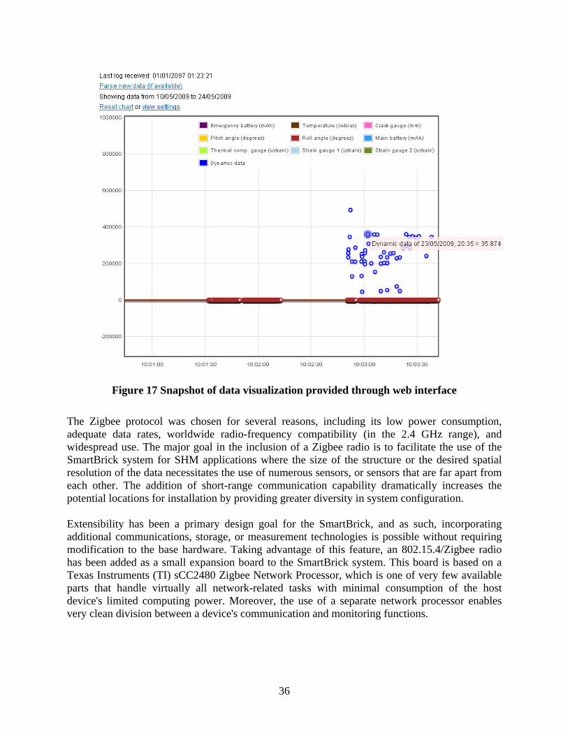
A block diagram depicting information flow in the SmartBrick network is provided in Figure 16. The base station and sensor nodes collect data from the onboard and external sensors. The sensor nodes communicate their data to the base station over the Zigbee connection. The base station processes this data and communicates it, along with any alerts generated, to a number of destinations over the GSM/GPRS link provided by the cellular phone infrastructure. The data is reported by email and FTP to redundant servers, via the Internet, at regular intervals, or on an event-triggered basis. The alerts are sent directly by SMS text messaging, and by email. A web-based graphical user interface (GUI) is provided for download of data and charts, supported by a processing backend. The data from each measured channel is compressed into eight bytes. Single-precision floating point representation is used. On the remote server, a daemon is used to populate a SQL database. Queries from the database are carried out using a Java/Silverlight interactive interface, which also generates charts for data visualization. Figure 17 provides an example where data from multiple sensors is represented in the same chart.
Figure 16 Block diagram of the SmartBrick structural health monitoring network
36
Figure 17 Snapshot of data visualization provided through web interface
The Zigbee protocol was chosen for several reasons, including its low power consumption, adequate data rates, worldwide radio-frequency compatibility (in the 2.4 GHz range), and widespread use. The major goal in the inclusion of a Zigbee radio is to facilitate the use of the SmartBrick system for SHM applications where the size of the structure or the desired spatial resolution of the data necessitates the use of numerous sensors, or sensors that are far apart from each other. The addition of short-range communication capability dramatically increases the potential locations for installation by providing greater diversity in system configuration. Extensibility has been a primary design goal for the SmartBrick, and as such, incorporating additional communications, storage, or measurement technologies is possible without requiring modification to the base hardware. Taking advantage of this feature, an 802.15.4/Zigbee radio has been added as a small expansion board to the SmartBrick system. This board is based on a Texas Instruments (TI) sCC2480 Zigbee Network Processor, which is one of very few available parts that handle virtually all network-related tasks with minimal consumption of the host device's limited computing power. Moreover, the use of a separate network processor enables very clean division between a device's communication and monitoring functions.

37
3.2 Evaluation Results
Laboratory testing of the Zigbee-enabled network comprised of a SmartBrick base station and the ez430-RF2480 evaluation modules has been previously reported. The SmartBrick was configured to interact with the modules over UART, which is the only interface available without requiring modification to the modules. The SmartBrick then configured the module as a coordinator and registered its application profile on the network, enabling the sensor boards to connect to it and report their measurements. The results were promising, despite the shortcomings of the evaluation boards, foremost of which is high power consumption. The same network was used to conduct subsequent open-air tests, using the evaluation modules in non-beaconing mode. The network was formed on channel 16 (0x10), operating at 2.43 GHz. Two different configurations were used. In the first configuration, a coordinator was directly connected to an end device located at a 10 m distance. In the second configuration, a router served as an intermediary, as shown in Figure 18. In both cases, the coordinator was connected to the SmartBrick via a UART port operating at 9.6 kbps. All data received by the Zigbee coordinator (ZC) was sent over this serial port to the SmartBrick and transmitted to the computer using another serial port operating at the same data rate.
Figure 18 One of two test configurations
All frames were parsed, and any frames containing application-related update messages from the sensor were saved to the SmartBrick’s EEPROM. A TI CC2430DB was used as a packet sniffer, with TI’s Packet Sniffer software v2.11.2, to observe the traffic and obtain timing information for the calculation of network throughput. The end device and the router were programmed to send update messages every three seconds, with an application payload of 20, 40, or 60 bytes. The three tests carried out are described below. Table 5 summarizes the results.

38
3.2.1 Test 1: Direct connection of coordinator and end device
A Zigbee network consisting of a ZC and an end device at a distance of 10 m from the ZC was formed, as described above. This distance was empirically found to be the approximate limit for data transmission by the end device at an acceptable rate. The packet sniffer was used to capture packets exchanged between the end device and the ZC. This data was observed for three minutes. The time required by the end device to transmit data to the ZC and receive an acknowledgement was used to calculate application throughput for varying application payloads. The device failed when an attempt was made to transmit a payload of 80 bytes.
3.2.2 Test 2: Indirect connection of coordinator and end device
A Zigbee network consisting of a ZC, a router at 7 m from the ZC, and an end device at 9 m from the router was formed, as depicted in Figure 18. The objective of testing this second configuration was investigating the effect of a adding a router to the network when the end device is operating very close to its maximum range. The packet sniffer was used to capture the packets exchanged between the end device and the router, and between the router and the ZC. This data was observed for three minutes. The time required by the end device to transmit data to the router, the time required to receive an acknowledgement from the router, the time required by the router to send the data packet to the ZC, and the time required to receive an acknowledgement from the ZC to the router were used to calculate application throughput for varying application payloads. The processing time at the router was assumed to be negligible.
3.2.3 Test 3: Direct connection of coordinator and end device (Burst Mode)
A Zigbee network consisting of a ZC and an end device at a distance of 10 m from the ZC was formed, as described above. The end device was programmed to transmit in burst mode, where a transmitting device begins to transmit as soon as it receives an acknowledgement from the receiver. The end device was allowed to transmit in burst mode for 10 seconds. This test was repeated for varying application payloads. The end device would stop transmitting after a few seconds of transmission. This is due to a safeguard mechanism that prevents the transmission of large data bursts that would block the network. The throughput observed is greater than that of non-burst mode, where the device goes to sleep in between transmissions, requiring additional time to wake the device and resume transmission. Acknowledgements are disabled in burst mode, and as such, the success ratio cannot be measured.
Table 5 Open-air test results
Test 1 Test 2 Test 3
Application payload (bytes) 20 40 60 20 40 60 20 40 60
Application throughput (bytes/sec) 145 206 345 125 245 320 2100 3018 3950
Success Ratio (Successful transmissions/Total frames) 57/60 56/60 58/60 60/60 58/60 60/60 N/A

39
The SmartBrick network continues to expand in capabilities and improve in performance. The system now has a reliable means of communicating with other nearby devices, and even with the limited capabilities of the ez430-RF2480 evaluation modules, was shown to sustain data rates sufficient for the SmartBrick network to communicate all of its measurements with a minor increase in overall power consumption. Short-range communication capability, combined with the extensive sensing capabilities of the SmartBrick, opens a world of possibilities for remote monitoring of structures, meaning that the system can be installed on virtually any structure, of any size. Laboratory and field testing of the Zigbee daughterboards designed as a replacement for the evaluation modules is planned for the immediate future. This dedicated hardware is expected to yield significant improvements in the reliability, range, and throughput of wireless communication, with only a marginal increase in power consumption.
3.3 Planned Instrumentation Layout
Three SmartBrick base stations and 12 nodes will be used to monitor over 50 strain gages placed along rebar in the structure. Additionally, several accelerometers and temperature sensors will be installed on the bridge to achieve an improved perspective on the bridge environment. The proposed sensor placement is shown in Figure 19. Sensors will be placed throughout the structure, at various heights and depths. Due to the bridge's unique construction, the measurements are intended to provide information on the behavior of the individual structural components, as opposed to the structure as a whole. The symmetry and pre-fabricated nature of the structure is exploited so that several sensors can be placed on one of many similar members and reduce the number of sensors required to assess the bridge.
Figure 19 Instrumentation layout

40
4 CONCLUDING REMARKS
This report summarizes the superstructure and instrumentation design of a three-span bridge with the use of fiber reinforced polymer bars in concrete decks and girders. The three spans include a precast box-girder bridge, a precast deck on steel girder and a precast deck on concrete girder. They were designed to meet the requirements in AASHTO Bridge Specifications and ACI440 Guidelines.
The performance of various bridge decks reinforced with fiber reinforced polymers (FRP) will be compared through field instrumentations. For this purpose, a wireless, fully autonomous monitoring system was designed to facilitate the collection of field data after the completion of bridge construction. The collected data will allow the study of FRP bars and stay-in-place FRP grid systems.

41
REFERENCES AASHTO, AASHTO LRFD Bridge Design Specifications, Customary U.S. Units, 4th Edition,
2007.
ACI 318-08, Building Code Requirements for Structural Concrete and Commentary, Reported by ACI Committee 318, 2008.
ACI 440.1R-06, Guide for the Design and Construction of Concrete Reinforced with FRP Bars, Reported by ACI Committee 440, 2006.
Hughes Brothers Inc., “Hughes Brothers Reinforcements” Product Guide Specification, Web site: http://www.hughesbros.com, 2003.
AISC, Steel Construction Manual, American Institute of Steel Construction, 13rd Edition, 2005.
Canadian Highway Bridge Design Code. CAN/CSA-S6-06. Canadian Standards Association, 2006
United States Federal Highway Administration. 2007. “Deficient Bridges by State and Highway System,” Available: http: //www.fhwa.dot.gov/bridge/defbr07.cfm.
Frangopol, D. M., A. Strauss, and S. Kim. 2008. “Bridge Reliability Assessment Based on
Monitoring,” J. Bridge Engineering, 20(3): 258–270. Zhou, Z., L. D. Wegner, and B. F. Sparling. 2007. “Vibration-Based Detection of Small-Scale
Damage on a Bridge Deck,” J. Structural Engineering, 133(9):1257–1267. Cheung, M. M. S., B. Noruziaan, and W. C. Li. 2004. “Data Acquisition, Processing and
Management Systems for a Canadian Bridge Monitoring project,” in International Conference on Computing in Civil and Building Engineering.
Harms, T., F. Bastianini, and S. Sedigh. 2008. “An Embedded Wireless System for Remote
Monitoring of Bridges,” presented at the 15th Int’l SPIE Symposium on Smart Structures and Materials and Nondestructive Evaluation and Health Monitoring, March 9-13, 2008.
Harms, T., B. Banks, S. Sedigh, and F. Bastianini. 2009. “Design and Testing of a Low-Power
Wireless Sensor Network for Structural Health Monitoring of Bridges,” presented at the 16th Int’l SPIE Symposium on Smart Structures and Materials and Nondestructive Evaluation and Health Monitoring, March 9-13, 2009.
Choi, H., S. Choi, and H. Cha. 2008. “Structural Health Monitoring System Based on Strain
Gauge Enabled Wireless Sensor Nodes,” in International Conference on Networked Sensing Systems.

42
APPENDIX: MORE DATA RELATED TO THE SPAN WITH STEEL GIRDERS
Figure 20 Leveling and grout pocket details


