DESIGN AND OPTIMIZATION OF A ONE-DEGREE...

DESIGN AND OPTIMIZATION OF A

ONE-DEGREE-OF-FREEDOM SIX-BAR LINKAGE

KLANN MECHANISM

A Project Report submitted in partial fulfilment of the requirements for

award of the degree of

BACHELOR OF TECHNOLOGY

In

MECHANICAL ENGINEERING

By

MADUGULA JAGADEESH (09VV1A0332)

YALAMATI VASU CHAITANYA KUMAR (09VV1A0360)

REDDIPALLI REVATHI (09VV1A0313)

Under the esteemed guidance of

Dr . N. MOHAN RAO, M .E, Ph.D.

Associate professor and Head of Mechanical Engineering Department Of Mechanical Engineering

Department Of Mechanical Engineering

UNIVERSITY COLLEGE OF ENGNEERING

JAWAHARLAL NEHRU TECHNOLOGICAL UNIVERSITY

KAKINADA

VIZIANAGARAM CAMPUS

2009-2013

CERTIFICATE

This is to certify that the project entitled “DESIGN AND OPTIMIZATION OF A ONE-DEGREE-OF-FREEDOM SIX-BAR LINKAGE, KLANN MECHANISM” is a bona fide work of

MADUGULA JAGADEESH (09VV1A0332), YALAMATI VASU CHAITANYA KUMAR (09VV1A0360), REDDIPALLI REVATHI (09VV1A0313), during the period 19

th February 2013 to 15

th April

2013 and is submitted in the partial fulfilment of the requirements

for the award of the degree in BACHELOR OF TECHNOLOGY IN MECHANICAL ENGINEERING from the JAWAHARLAL NEHRU TECHNOLOGICAL UNIVERSITY KAKINADA, UNIVERSITY COLLEGE OF ENGNEERING VIZIANAGARAM.

Dr.N.MOHAN RAO, M.E., Ph.D.

Associate professor &

Head of Mechanical Engineering

J.N.T.U.K.UNIVERSITY COLLEGE OF ENGNEERING

VIZIANAGARAM.

ACKNOWLEDGMENT

It is needed with a great sense of pleasure and

immense sense of gratitude that we acknowledge the help of these

individuals. We owe many thanks to many people who helped

and supported us during the writing of this report.

We would like to express our deep sense of gratitude

and regards to Dr. N.MOHAN RAO, M.E, Ph.D & Head of

Mechanical Department, who initiated in taking up this

project work. We are grateful to his persisting encouragement and

valuable guidance in completing our project work successfully.

We are thankful to his everlasting patience and valuable

suggestions throughout my project work.

We express our sincere thanks to our respected

Prof.P.UDAYA BHASKAR, Principal of JNTUK, College of

Engineering.

We are thankful to all faculty members for extending

their kind cooperation and assistance. Finally, we are extremely

thankful to our parents and friends for their constant help and

moral support.

TABLE OF CONTENTS

Chapter-1 INTRODUCTIION

1.1 Introduction

1.2 Literature Survey

1.3 Objectives of Present Work

Chapter-2 KLANN LINKAGE

2.1 Introduction

2.2 Description

2.3 Design of Linkage

2.4 Analysis of walking motion

2.5 Advantages and disadvantages of Klann linkage

over wheels or tracks

2.5.1 Advantages

2.5.2 Disadvantages

2.6 Applications of Klann Linkage

Chapter-3 SYNTHESIS

3.1 Introduction to Synthesis

3.2 Type, Number and Dimension Synthesis

3.3 Graphical and Analytical Synthesis

3.3.1 Graphical Synthesis

3.3.2 Analytical Synthesis

Chapter-4 SYNTHESIS OF KLANN LINKAGE

4.1 Position Analysis of Klann Linkage

4.2 C Program for Locus Co-ordinates

Chapter-5 OPTIMIZATION

5.1 Introduction

5.2 Dimensional Synthesis of Klann Mechanism through

Optimization

5.3 Genetic Algorithm

5.4 Formulation of Objective Function

5.5 Steps followed in calculating optimized link lengths for a

certain Step Length and Height

Chapter-6 CALCULATIONS AND RESULTS

6.1 Table of arbitrary link lengths and target co-ordinates

6.2 Output of Genetic Algorithm

6.3 Table comparing the target and generated co-ordinates

Chapter-7 CONCLUSIONS

Chapter-8 REFERENCES

Page | 1

Chapter-1

1.1 Introduction:

It has been established that off-road vehicles with legs exhibit better

mobility, obtain higher energy efficiency and provide more comfortable

movement than those of conventional tracked or wheeled vehicles while

moving on rough terrain. So there is necessity to analyse & develop these

leg mechanisms in order to meet various applications. Klann mechanism

is one of these leg mechanisms which consists of six-links which is used

as an alternative for wheels. Each wheel is replaced by two Klann

mechanisms whose cranks are 180 degrees out of phase. To provide

mobility for the mechanism required number of links and dimensional

synthesis of links is required. This mechanism is used as a replacement of

wheels finds applications in planetary exploration, walking chairs for the

disabled and for military transport, rescue in radioactive zones for nuclear

industries and in other hostile environments.

1.2 Literature Survey:

In 1770, Richard Edgeworth tried to construct a wooden horse with 8 legs

to jump over high walls however 40 years of experimentation was

unsuccessful in constructing such a mechanism.

In 1968, General Electric developed a walking truck that was capable of

walking 5 mph and in 1976, Frank and McGhee made the first computer

controlled walking machine. More recently, a Mechatronics Research

Group from the University of Southern Queensland created a

pneumatically powered quadruped and Applied Motion Inc, created a

Spring Walker bipedal exoskeleton.

Type synthesis has been one of the focuses for the early research on

design of leg mechanisms, where slider-crank mechanisms and multiple

cam mechanisms have been used. It was recommended to use only

revolute joints for leg walking machines due to the difficulties in

lubrication and sealing of the sliding joints, which is essential for the

machines to walk outdoors. Many pin-joined legged mechanisms have

been designed, which are often compound mechanisms consisting of a

four-bar linkage and a pantograph. The potential advantages of such

compound mechanisms are fast locomotion, minimal energy loss,

simplicity in control design, and the slenderness of the leg.

There have been many investigations on the adequate degrees-of-freedom

(DOF) for each leg mechanism. Depending on the desired functional

Page | 2

requirements (flexibility, speed, etc.) and walking environment, the

legged walkers can have up to eight legs and a total of eighteen active

DOF.

Another example is the adaptive Suspension vehicle developed by Ohio

State University, which has six legs and eighteen DOF. In general, it has

been accepted that three DOF for each leg is required to provide high

mobility, one for providing back-and-forth, one for up-and-down motion

of the foot and one for turning.

However, it has been discussed that unlike a ground-based manipulator

that can be operated with an off-board power supply, a walking machine

has to carry the entire power supply in addition to the external payload

and the weight of the machine body. Thus, it is desirable to use a small

number of actuators to reduce the body weight and to simplify the motion

coordination. A number of six-link and seven-link leg mechanisms have

been designed with one degree-of-freedom. Rigorous research has been

carried out on their mobility and energy loss through kinematic and

structural analysis.

Two important findings have been documented:

A crank as an input link with continuous rotation motion should be

used to achieve fast motion with minimum control

An ovoid foot path is necessary to step over small obstacles without

raising the body too much height.

These two requirements are important for designing single-DOF leg

mechanisms for mobility and energy efficiency.

1.3 OBJECTIVES OF PRESENT WORK

Many techniques for the synthesis of linkages are invented in recent

years. Most of these approaches are involved techniques and are

mathematically complicated. Only few of them allow a closed from

solution. Of these, optimization procedures attempting to minimize an

objective function play an important role.

A set of inequality constraints that limit the range of variation of

parameters may be included in the calculation. The new values of linkage

parameters are generated with each iteration step according to particular

optimization scheme used. The closest achievable fit between the

calculated points and desired points is sought. Even the desired points will

Page | 3

not exactly match but this is considered as acceptable result for most

engineering tasks.

Each optimization approach has as own advantages and disadvantages in

term of convergence accuracy, reliability, complexity and speed. Some

methods converge even to a minimum value of objective they may not be

the best solution. Based on this points there is a lot of scope for

application of new methods of optimization for six-bar synthesis problem.

Following are the main objective of the present work:

(1) Path synthesis of Klann mechanism.

(2) Implementation of genetic algorithm optimization scheme.

(3) Compare the obtained locus with the desired locus and finding offset

to each precision point.

Page | 4

Chapter-2

KLANN LINKAGE

2.1 Introduction:

Linkages can be made to provide almost any movement required these

movements can often be quite complex, but few linkages can match the

complexity of those walking linkages created by nature-legs. Joseph

Klann emulated the complex movement of linkages which is similar to

the movement natural gait.

The klann linkage is a open loop six-bar planar mechanism designed to

simulate the gait of legged animal and function as a wheel replacement.

The six-bar klann linkage is an expansion of the four-bar Burmester

linkage developed in 1888 for harbour cranes. Each wheel is replaced by

two legs.

2.2 Description:

Each leg consists of a Klann linkage consists of the frame, a crank,

two grounded rockers, and two couplers all connected by pivot

joints that converts rotating motion into linear motion.

Each leg of a Klann linkage includes a frame which supports a

walking assembly composed of a cooperative arrangement of

linkages axially connected together so as to provide a walking

assembly which simulates the walking gait of an animal.

Klann linkage

The linkages are approximately linked together by axial linking

means for axially connecting the linkages together and to the frame.

Page | 5

The linkages include a pair of rocker arms (upper and lower)

axially mounted to a frame, a connecting arm or rod, a

reciprocating leg and a cranking link.

The pair of rocker arms includes a first rocker arm(upper) and a

second rocker arm(lower) respectively axially anchored at one of

their respective rocker arm ends to the frame and to different

linkages at an opposite rocker arm end.

2.3 Design of Linkage:

Final design for a Klann linkage interactive model. There are actually two Klann

linkages in parallel, oriented 180 degrees out of phase and stacked vertically.

The two linkages (crankshafts) had to be held 180 degrees out of

phase. The Klan linkage has a purely rotational input about a

stationary point. The input can be seen as the two out-of-phase

short links in the above figure.

These two input links create a sort of crankshaft that drives the

linkage motion. If the point about which the crankshaft rotated had

Page | 6

a pin going all the way down to the mounting plate, the lower

Klann linkage would collide with this pin.

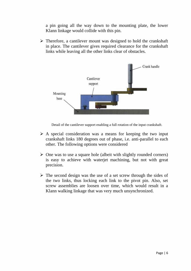
Therefore, a cantilever mount was designed to hold the crankshaft

in place. The cantilever gives required clearance for the crankshaft

links while leaving all the other links clear of obstacles.

Detail of the cantilever support enabling a full rotation of the input crankshaft.

A special consideration was a means for keeping the two input

crankshaft links 180 degrees out of phase, i.e. anti-parallel to each

other. The following options were considered

One was to use a square hole (albeit with slightly rounded corners)

is easy to achieve with waterjet machining, but not with great

precision.

The second design was the use of a set screw through the sides of

the two links, thus locking each link to the pivot pin. Also, set

screw assemblies are loosen over time, which would result in a

Klann walking linkage that was very much unsynchronized.

Page | 7

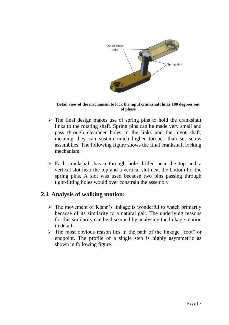
Detail view of the mechanism to lock the input crankshaft links 180 degrees out

of phase

The final design makes use of spring pins to hold the crankshaft

links to the rotating shaft. Spring pins can be made very small and

pass through clearaner holes in the links and the pivot shaft,

meaning they can sustain much higher torques than set screw

assemblies. The following figure shows the final crankshaft locking

mechanism.

Each crankshaft has a through hole drilled near the top and a

vertical slot near the top and a vertical slot neat the bottom for the

spring pins. A slot was used because two pins passing through

tight-fitting holes would over constrain the assembly

2.4 Analysis of walking motion:

The movement of Klann’s linkage is wonderful to watch primarily

because of its similarity to a natural gait. The underlying reasons

for this similarity can be discerned by analysing the linkage motion

in detail.

The most obvious reason lies in the path of the linkage “foot” or

endpoint. The profile of a single step is highly asymmetric as

shown in following figure.

Page | 8

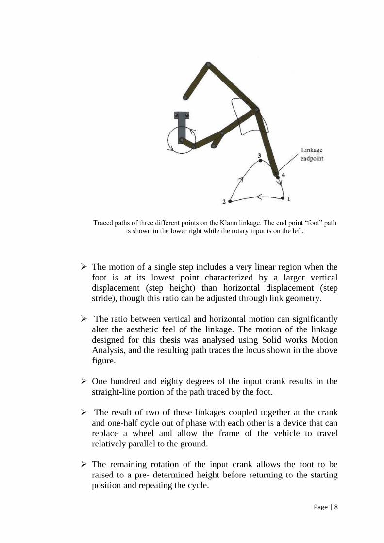
Traced paths of three different points on the Klann linkage. The end point “foot” path

is shown in the lower right while the rotary input is on the left.

The motion of a single step includes a very linear region when the

foot is at its lowest point characterized by a larger vertical

displacement (step height) than horizontal displacement (step

stride), though this ratio can be adjusted through link geometry.

The ratio between vertical and horizontal motion can significantly

alter the aesthetic feel of the linkage. The motion of the linkage

designed for this thesis was analysed using Solid works Motion

Analysis, and the resulting path traces the locus shown in the above

figure.

One hundred and eighty degrees of the input crank results in the

straight-line portion of the path traced by the foot.

The result of two of these linkages coupled together at the crank

and one-half cycle out of phase with each other is a device that can

replace a wheel and allow the frame of the vehicle to travel

relatively parallel to the ground.

The remaining rotation of the input crank allows the foot to be

raised to a pre- determined height before returning to the starting

position and repeating the cycle.

Page | 9

The motion path of a single step is a very interesting shape.

However, the shape provides, only a part of the linkage motion.

The speed of the linkage “foot” at various points in a single step is

also both important and intriguing.

The endpoint velocity (magnitude) is a function of the input crank

angle for a constant rotational velocity input. The input angle is

measured counter-clockwise from the horizontal. The locations

along the step path shown in above figure.

The maximum velocity occurs as the foot is coming down for the

next step (point 4), giving the marching effect in the linkage’s gait.

It is also interesting to note that the minimum velocity occurs both

at the beginning of a stride and also at the end (points 1&2).

The endpoint velocity goes through a local minimum at the peak of

the step height (point3), creating a wonderful hesitation in the

linkage motion before the rapid and dramatic downward step.

It is the combination of the asymmetric endpoint path and the

highly variable endpoint velocity that creates the fluid stepping

motion so characteristic of Klann’s linkage.

2.5 Advantages and disadvantages of Klann linkage over

wheels or tracks:

2.5.1 Advantages:

Walking vehicles have many advantages over wheeled toe tracked

vehicles. These may be listed as follows:

Contact with the ground at discrete points:

The rims of wheels have continuous contact with the ground over which

they travel. Walking machines place their feet and once placed, frictional

forces prevent further movement of the foot and movement is confined

within the linkage system of the leg. The dynamics of the vehicle body is

determined by the leg kinematics alone, whereas in wheeled vehicles, the

body position is continuously affected by the contour of the road surface.

Vehicle suspension mitigates this effect on modern vehicles, but it is

entirely eliminated in walking machines.

Page | 10

Elimination of roads: Although heavy usage would lead to tracks forming, as found when

animals move along the same path regularly, walking machines do not

require roads or other prepared surface to walk on. With light traffic, a

legged vehicle should leave only a series of discrete footprints.

Minimal contact area with ground: In number of footprints per distance travelled. This is considerably less

than the area moved over by a wheeled or tracked vehicle, which is the

width of tyre or track times the distance travelled. For example, in an area

of land where land mines have been randomly deployed. The continuous

track of a wheeled vehicle increases the chance of a land mine being

trigged. Whereas a walker touches a much smaller area of the land over

which it travels, and there would be reduced risk of triggering mines,

walking machines, the total ground area touched is the area of each

footprint times the

Reduced ground pressure:

As a walking machine may carry a foot of practically any size, the

average ground pressure it exerts can be very small. In wheeled vehicles

the diameter of the wheels places a physical limit on the length of the

footprint. Although tyres can be made wide, the maximum contact patch

size is limited, and ground pressure cannot easily be reduced below a

certain value. Tracked vehicles can have a large contact area, and hence

are preferred where low ground pressure is advantageous, for example

vehicles that operate in snow or swamps. A walking machine could be

competitive with a tracked vehicle in these conditions, although this still

depends on the reduced body weight that could result from improved

design of walkers.

Vehicle height: If a walking machine has a mammalian type body plan, with the legs

attached underneath its body, then the body is carried higher off the

ground than the body of a conventional wheeled or tracked vehicle would

be. This body position may be advantageous where the vehicle is intended

as a moveable vantage point, for example in game viewing applications.

Greater vehicle height would also enhance wading abilities.

Increased traction: Wheeled vehicles are subject to slip, especially when applying high

tractive effort on loose slippery or wet surfaces. A suitable walking

machine, with sharp feet to increase ground pressure, and hence

Page | 11

penetration, could apply more tractive effort than a wheeled vehicle. It

may not be able to compete with a tracked vehicle however other types of

feet that firmly attach to the walking surface could also be employed to

allow increased traction

Amphibious potential: With a suitable leg arrangement carrying a set of floats or pontoons, a

walking machine could be made an effective amphibious vehicle. If the

area of float can be made large enough, then vertical displacement of the

weight carrying floats can be less than the foot lift of the returning leg.

This means the vehicle could walk on the surface of water, as returning

floats would be lifted clear of the water surface, and placed forward of the

current float. Such a vehicle should also walk on land, with extremely low

ground pressure.

Climbing abilities: With the addition of suitable foot attachment devices, such as electro-

magnets for steel surfaces or suction devices for smooth surfaces, such as

glass, it should be possible to make a walking machine travel vertically or

even upside down. The foot attachment mechanism would need to have

grip control, releasing grip to allow the leg to be lifted on the return stroke

and acquiring it when the leg is on its duty cycle.

2.5.2 Disadvantages: The fact that vehicles that use wheels or tracks are the only types of

vehicles currently being constructed in any significant numbers, and given

that many attempts have been made to create walking machines, there

must be severe disadvantages to using walking machines for

transportation. These include:

Complication: Wheels are extremely simple, in the simplest form, a circular plate with a

central hole. The wheel is widely considered one of human kind’s greatest

inventions. It is probably the simplest device that can be used for land

transportation.

Walking vehicles are generally orders of magnitude more complex. There

are many joints, kinematic links, sensors, software, multiple actuators,

difficult manoeuvrability issues and stability issues that all make most

current walking machines more complex.

Page | 12

Inefficiency: Walking machines are not fuel-efficient, especially considering the slow

speeds at which they travel. Wheels running on a good road surface are

the most efficient way to travel on land.

Tracks are considerably less efficient than wheels. This is primarily due to

the energy required to move the track itself. The large number of revolute

joints connecting the track sections, with their associated friction, means

that simply turning a track absorbs considerable power.

Although it is hard to accumulate data or find a means of comparing

tracks to kegs in terms of transport efficiency, a brief consideration would

indicate that walking machines could be made to be similar in efficiency

to tracked vehicles.

Cost: The cost of construction will generally be related to its complexity. Given

the complexity of most current walkers it is not surprising that none has

entered production, as presumably they could not be sold at a reasonable

price

However, tracked vehicles are also extremely costly in relation to wheeled

ones. Even specialist wheeled vehicles command a premium price. If a

sufficiently simple hence cheap walking machine could be constructed,

and located in specific marketing and operational niches, it may be

possible to sell these at a competitive price.

2.6 Applications of Klann linkage:

The final design of this new walking machine is intended for transport

service across rough terrain. It should be large enough to carry a

significant payload, of some tons. It should be capable of operating

without roads, and should be self-sufficient with respect to motive power.

The envisaged operating environment would be somewhat flat land, such

as open bush country, or light forest. It should be capable of ascending

and descending slopes of up to 400, and should be sufficiently

manoeuvrable to avoid large obstacles. It should be able to move at

reasonable walking speeds, up to 50 kilometres per hour and have a

useable range of several hundred kilometres before refuelling. It should

be robust, simple and easy to maintain. Complex parts that cannot be

repaired in the field should be minimized.

The two legs in Klann linkage coupled together at the crank can act

as a wheel replacement and provide vehicles with greater ability to

Page | 13

handle obstacles and travel across uneven terrain while providing a

smooth ride.

This linkage could be utilized almost anywhere a wheel is

employed from small wind-up toys to large vehicles capable of

transporting people.

Initially the linkage was called spider bike but applications for this

linkage have expanded well beyond the initial design purpose of a

human-powered walking machine.

Other practical applications could include:

1. Forestry applications,

2. Land mine clearing,

3. Game viewing,

4. Off-road use in areas where roads are undesirable e.g. in game

parks,

5. Transportation across snow or ice,

6. Travel in swampy areas, and

7. Travel on beaches or sandy areas.

Page | 14

Chapter-3

SYNTHESIS

3.1 Introduction:

Synthesis of mechanism refers to design a linkage for a prescribed motion

or path or velocity of tracing joint or link there are types of synthesis

technique available in literature.

The following methods of synthesis are commonly found in literature

1. Qualitative synthesis, which is a creation of potential solution in

the absence of an algorithm that configures or predicts solution

2. Type synthesis, which is a definition of proper type of

mechanism best suited to the problem and is a form of

qualitative synthesis

3. Dimensional synthesis, referring to the determination of lengths

of links necessary to accomplish the desired motion.

3.2 TYPE, NUMBER AND DIMENSION SYNTHESIS:

Type synthesis refers to the kind of mechanism selected it might be

a linkage, a geared system, belts and pulleys, or even a cam system.

This beginning phase of the total design problem usually involves

design factors such as manufacturing processes, materials, safety,

space, and economics. The study of kinematics is usually only

slightly involved in type synthesis.

Number synthesis deals with the number of links and the number

of joints or pairs that are required to obtain certain mobility.

Number synthesis is the second step in the design.

The third step in design namely determining the dimensions of the

individual links is called dimensional synthesis.

We mainly concentrate on the dimensional synthesis since the

main objective of this thesis is the calculation of link lengths.

Page | 15

Following are various problems occurring in dimensional synthesis.

a) Function Generation

A frequent requirement in design is that of causing an output member to

rotate, oscillate, or reciprocate according to a specified function of time or

function of the input motion. This is called function generation. That is

correlation of an input motion with an output motion in a linkage. A

simple example is that of synthesizing a four-bar linkage to generate the

function the function y=f(x). In this case, x would represent the motion

(crank angle) of the input crank, and the linkage would be designed so

that the motion (angle) of the output rocker would approximate the

function y. Other examples of function generation are as follows: In a

conveyor line the output member of a mechanism must move at the

constant velocity of the conveyor while performing some operation for

example, bottle capping, return, pick up the cap, and repeat the operation.

The output member must pause or stop during its motion cycle to provide

time for another event. The second event might be a sealing, stapling, or

fastening operation of some kind. The output member must rotate at a

specified no uniform velocity function because it is geared to another

mechanism that requires such a rotating motion.

b) Path generation

A second type of synthesis problem is called path generation. This refers

to a problem in which a coupler point is to generate a path having a

prescribed shape that is controlling a point in a plane such that it follows

some prescribed path. Common requirements are that a portion of the path

be a circular arc, elliptical, or a straight line. Sometimes it is required that

the path cross over itself. For this minimum 4-bar linkage are needed. It is

commonly to arrive a point at a particular location along the path

without/with prescribed times.

c) Motion Generation

The third general class of synthesis problem is called body guidance. Here

we are interested in moving an object from one position to another. The

problem may call for a simple translation or a combination of translation

and rotation. In the construction industry, for example, heavy parts such

as a scoops and bulldozer blades must be moved through a series of

prescribed positions.

d) Hybrid Task synthesis

Certain applications may not be represented by a single task. It is

conceivable that a task may require an object to be moved along a

trajectory on which the orientation of the object may be important at a

Page | 16

few points, while restriction on orientation could be relaxed at others.

Furthermore, the task may require that a functional input/output relation

exists at a few points along the trajectory. This scenario calls for hybrid

task synthesis. The main benefit from a mechanism that performs a hybrid

task is that the entire motion cycle becomes active, that is, during a single

crank rotation the same mechanism can be used to perform several

subtasks simultaneously. For example, the task may dedicate a portion of

the trajectory to advancing an object along a path, another portion to

moving an object from one conveyor to another through several positions

while maintaining a desired orientation, and yet another segment to

generating a functional relationship between the drive and follower links,

as each may actuate valves that dispense prescribed amounts of different

materials in a single package.

3.3 GRAPHICAL AND ANALYTICAL SYNTHESIS:

Path generation is a subset of motion generation problem. Path generation

of linkage is relatively an important problem in robotics and electronics

industry. In path generation, the points prescribed for successive locations

of coupler link in the plane are known as precision points. The number of

precision points which can be synthesized is limited by the number of

equation available for solution. Four-bar linkage can be synthesized by

closed-form method up to 5 precision points for path generation with

prescribed timing. Basic path synthesis problem starts with two prescribed

points. There are both graphical and analytical methods available for path

generation problem. Available graphical and analytical techniques are

briefly explained in this section.

3.3.1 Graphical Synthesis

a) Two position synthesis:

Consider a four-bar linkage design in which link AB moves from A1B1 to

A2B2. To handle the problem graphically, draw the link AB in its two

positions A1B1 and A2B2.

Page | 17

Two position synthesis (coupler motion)

Draw construction lines from A1 to A2 and from B1 to B2. Bisect the line

A1A2 and B1B2 and extend the perpendicular bisector in convenient

directions. Select a convenient point on each bisector as fixed pivots O2 &

O4. Connect O2 with A1 and call it as link 2 and connect O4 with B1 and

call it as link 4. The line A1B1 is link-3, while OO4 is link-1. Check the

Grashof’s condition and repeat above steps if not satisfied. The graphical

procedure employed for the two-position synthesis problem can be

extended to the three position synthesis. As the number of precision points

to be traced increases, the graphical method fails to give a correct

solution.

b) Three position synthesis:

The synthesis of four bar mechanism consists of determining the

dimensions of the links in which the output link is to occupy three

specified positions corresponding to the three given positions of the input

link. Fig. (a)shows the layout of a four bar mechanism in which the

starting angle of the input link AB1 (link 2) of known length is .

Let 12, and 13 be the angles between the positions B1B2, B1B3 and

B1B3 measured anticlockwise. Let the output link DC1 (link 4) passes

through the desired positions C1, C2 and C3 and 12, 23 and 13 are the

corresponding angles between the positions C1C2, C2C3 and C1C3. The

length of the fixed link (link 1) is also known. Now we are required to

determine the lengths of links B1C1 and DC1 (i.e. links 3 and 4) and the

starting position of link 4 ( ).

The easiest way to solve the problem is based on inverting the mechanism

on link 4. The procedure is discussed as follows:

Page | 18

1. Draw AD equal to the known length of fixed link, as shown in Figure (b)

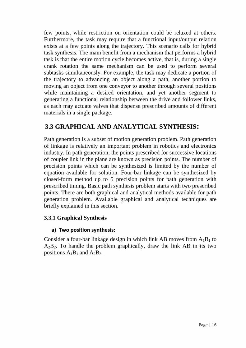
2. At A, draw the input link 1 in its three specified angular positions AB1, AB2 and AB3.

3. Since we have to invert the mechanism on link 4, therefore draw a line B2D and rotate it clockwise (in a direction opposite to the direction in which link 1 rotates) through an angle (i.e. the angle of the output link 4 between the first and second position) in order to locate the point B2

’.

Fig. a Layout of four bar mechanism

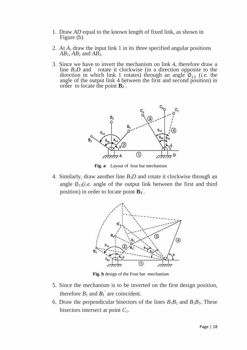
4. Similarly, draw another line B3D and rotate it clockwise through an

angle 13(i.e. angle of the output link between the first and third

position) in order to locate point B3’.

Fig. b design of the Four bar -mechanism

5. Since the mechanism is to be inverted on the first design position,

therefore B1 and B1’ are coincident.

6. Draw the perpendicular bisectors of the lines B1B2 and B2B3. These

bisectors intersect at point C1.

Page | 19

7. Join B1’C1 and C1D. The figure AB1”C1D is the required four bar

mechanism. Now the length of the link 3 and length of the link 4

and its starting position ( ) are determined. 3.3.2 Analytical synthesis:

An analytical method of synthesis, amenable to computer programming, is preferred whenever

1. A high level of accuracy is desired

2. A large number of configurations have to be solved 3. The graphical methods fail.

In this method, every link length and slider displacement (from a suitable

reference point) are represented by two-dimensional vectors expressed

through complex exponential notation. Considering each independent

closed loop in the mechanism, a vector equation (complex) is established.

Separating the real and imaginary parts of all these vector equations, a

sufficient number of nonlinear algebraic equations are obtained to solve

for the unknown quantities. Generally, these nonlinear equations can be

solved numerically using a computer. However, for some simple and

useful mechanisms, the nonlinear equations can be solved analytically in

closed form.

Let us consider 4R linkage (figure (a)) of given link lengths where i =

1, 2, 3, and 4. The configuration of the input link l1 is also prescribed by

the angle and we have to determine the configurations of the other two

links, namely, the coupler and the follower, expressed by the angles

and .

Referring to figure, all links are denoted as vectors, viz., , , and .

All angles are measured counter clock-wise from the X-axis

Page | 20

Fig. (a)

- - =

For rocker angle ( ) in Loop-1:

Expanding the above expression and equating the real and imaginary

parts we get the following equations:

For eliminating squaring and adding the above two equations we get:

Rearranging the above equation and expressing in the form of

a +b =c we get:

( )=

a= ( )

b= (

c= ( )

To solve for , without ambiguity of quadrant, it is better to substitute

Page | 21

in a +b =c we get :

(b+c)

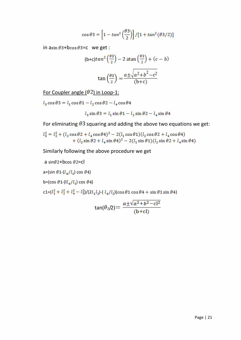
For Coupler angle ( ) in Loop-1:


Similarly following the above procedure we get

a sin +bcos =cl

a=(sin -( ) cos )

b=(cos -(l ) cos )

c1=( )/(2 )-( )( )

tan( 2/2)

Page | 22

Chapter 4

SYNTHESIS OF KLANN LINKAGE

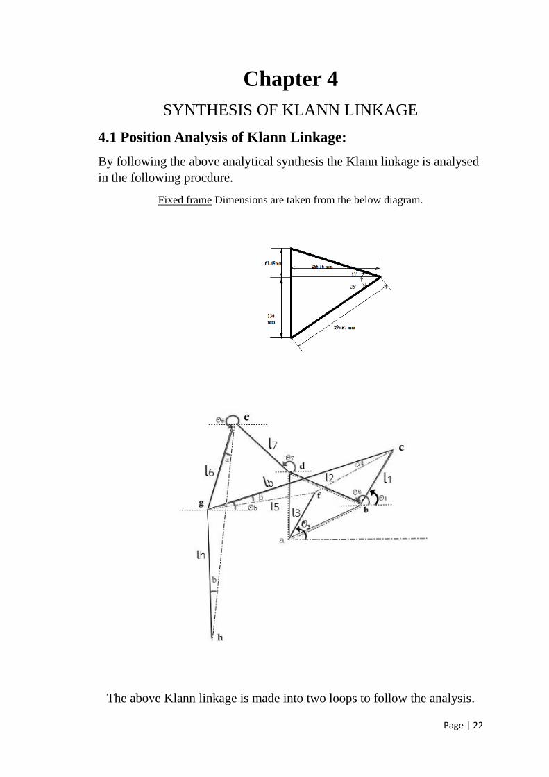
4.1 Position Analysis of Klann Linkage:

By following the above analytical synthesis the Klann linkage is analysed

in the following procdure.

Fixed frame Dimensions are taken from the below diagram.

The above Klann linkage is made into two loops to follow the analysis.

Page | 23

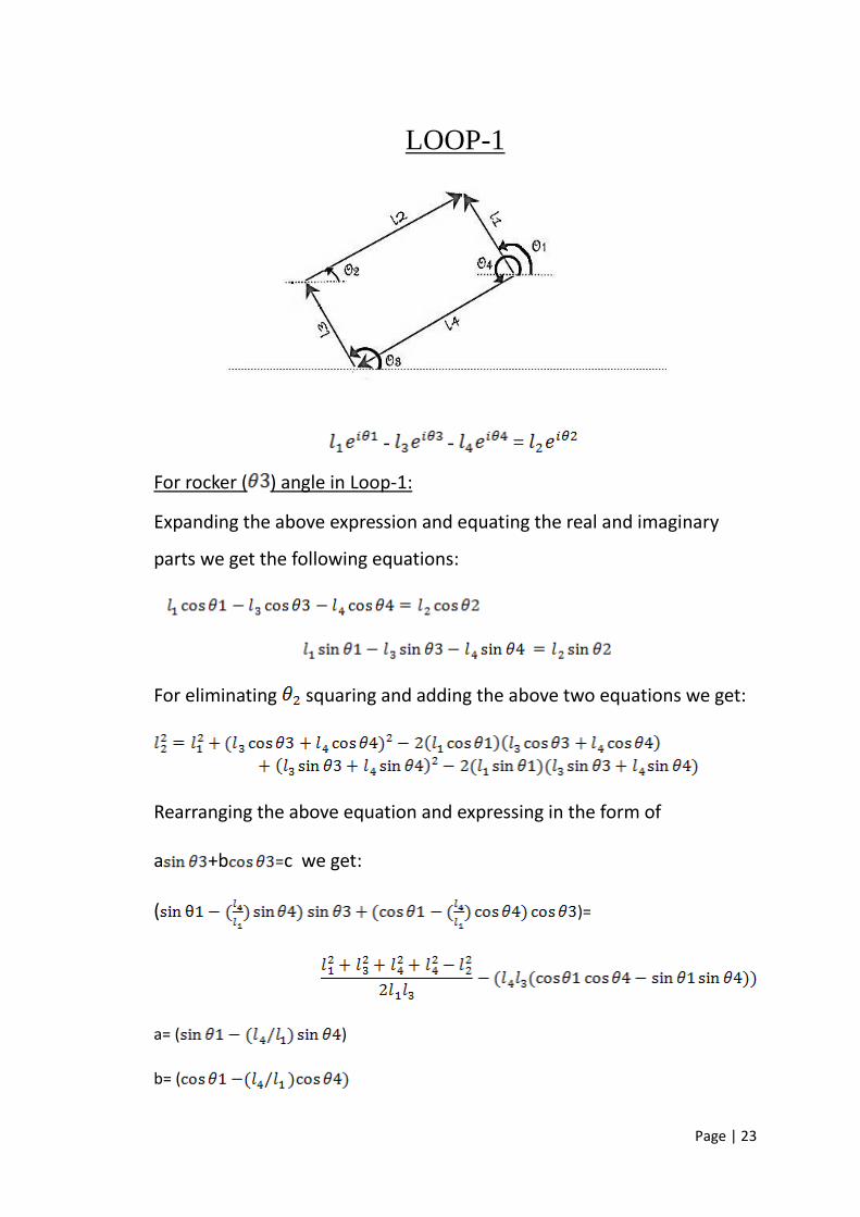
LOOP-1

- - =

For rocker ( ) angle in Loop-1:





a +b =c we get:

( )=

a= ( )

b= (

Page | 24

c= ( )

To solve for , without ambiguity of quadrant, it is better to substitute

in a +b =c we get :

(b+c)

For Coupler ( 2) angle in Loop-1:



a sin +bcos =cl

a=(sin -( ) cos )

b=(cos -(l ) cos )

c1=( )/(2 )-( )( )

tan( 2/2)

Page | 25

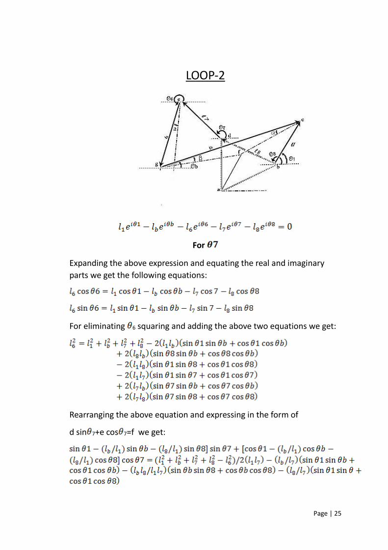
LOOP-2

For



For eliminating 6 squaring and adding the above two equations we get:


d sin 7+e cos 7=f we get:

Page | 26

d=

e=

f=

To solve for 7, without ambiguity of quadrant, it is better to substitute

sin 7=2tan( 7/2)/[1+tan2( 7/2)],

cos 7=[1- tan2( 7/2)]/[1+ tan2( 7/2)]

in dsin 7+ecos 7=f we get :

(e+f)tan2( 7/2)-2dtan( 7/2)+(f-e)=0

tan( 7/2)

For 6

For eliminating 7 squaring and adding the above two equations we get:


dsin 2+ecos 2=fl

d=

e=

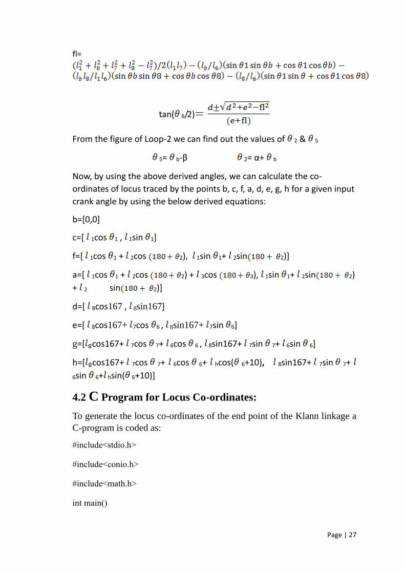
Page | 27

fl=

tan( 6/2)

From the figure of Loop-2 we can find out the values of 2 & 5

5= b-β 2= α+ b

Now, by using the above derived angles, we can calculate the co-

ordinates of locus traced by the points b, c, f, a, d, e, g, h for a given input

crank angle by using the below derived equations:

b=[0,0]

c=[ 1cos 1 , 1sin 1]

f=[ 1cos 1 + 2cos 2), 1sin 1+ 2sin 2)]

a=[ 1cos 1 + 2cos 2) + 3cos 3), 1sin 1+ 2sin 2)

+ 2 sin 2)]

d=[ 8cos167 , 8sin167]

e=[ 8cos167+ 7cos 6 , 8sin167+ 7sin 6]

g=[ cos167+ 7cos 7+ 6cos 6 , 8sin167+ 7sin 7+ 6sin 6]

h=[ cos167+ 7cos 7+ 6cos 6+ hcos( 6+10), 8sin167+ 7sin 7+

6sin 6+ hsin( 6+10)]

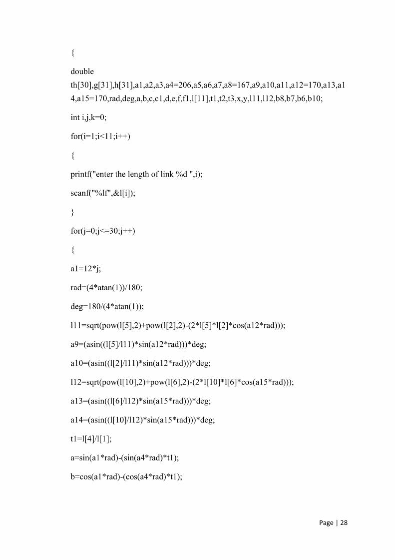
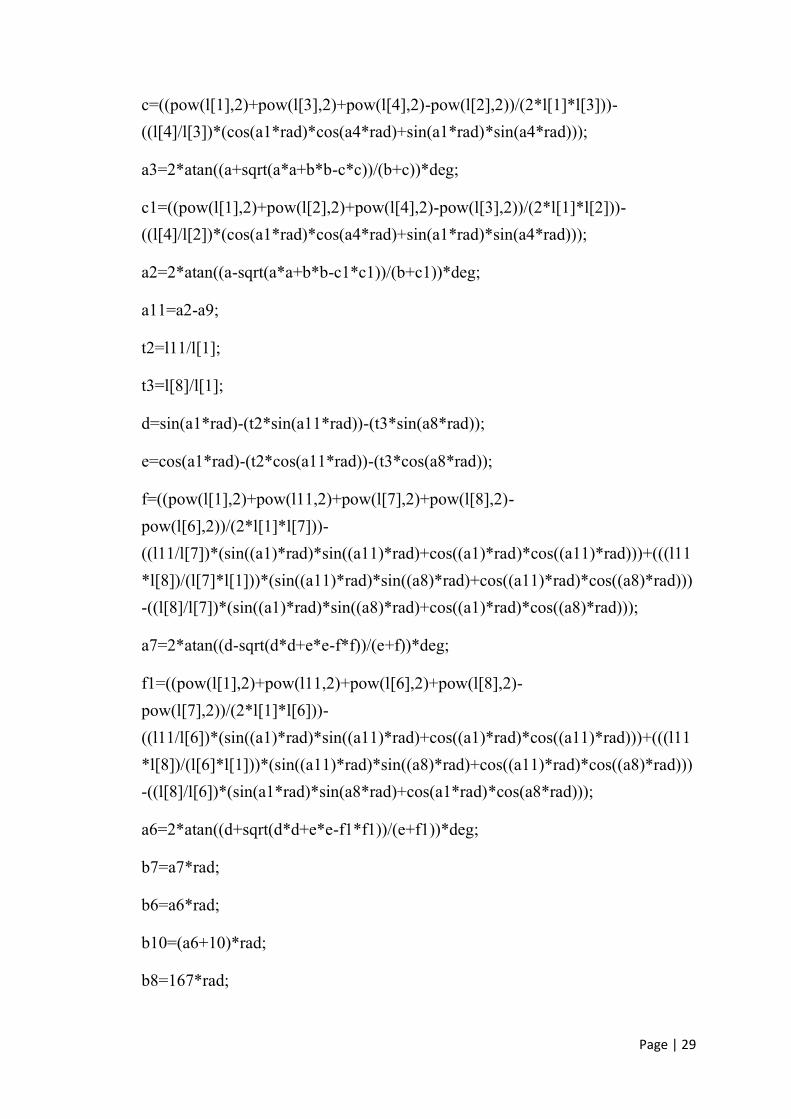
4.2 C Program for Locus Co-ordinates:

To generate the locus co-ordinates of the end point of the Klann linkage a

C-program is coded as:

#include<stdio.h>

#include<conio.h>

#include<math.h>

int main()

Page | 28

{

double

th[30],g[31],h[31],a1,a2,a3,a4=206,a5,a6,a7,a8=167,a9,a10,a11,a12=170,a13,a1

4,a15=170,rad,deg,a,b,c,c1,d,e,f,f1,l[11],t1,t2,t3,x,y,l11,l12,b8,b7,b6,b10;

int i,j,k=0;

for(i=1;i<11;i++)

{

printf("enter the length of link %d ",i);

scanf("%lf",&l[i]);

}

for(j=0;j<=30;j++)

{

a1=12*j;

rad=(4*atan(1))/180;

deg=180/(4*atan(1));

l11=sqrt(pow(l[5],2)+pow(l[2],2)-(2*l[5]*l[2]*cos(a12*rad)));

a9=(asin((l[5]/l11)*sin(a12*rad)))*deg;


l12=sqrt(pow(l[10],2)+pow(l[6],2)-(2*l[10]*l[6]*cos(a15*rad)));



t1=l[4]/l[1];

a=sin(a1*rad)-(sin(a4*rad)*t1);

b=cos(a1*rad)-(cos(a4*rad)*t1);

Page | 29

c=((pow(l[1],2)+pow(l[3],2)+pow(l[4],2)-pow(l[2],2))/(2*l[1]*l[3]))-

((l[4]/l[3])*(cos(a1*rad)*cos(a4*rad)+sin(a1*rad)*sin(a4*rad)));

a3=2*atan((a+sqrt(a*a+b*b-c*c))/(b+c))*deg;

c1=((pow(l[1],2)+pow(l[2],2)+pow(l[4],2)-pow(l[3],2))/(2*l[1]*l[2]))-

((l[4]/l[2])*(cos(a1*rad)*cos(a4*rad)+sin(a1*rad)*sin(a4*rad)));

a2=2*atan((a-sqrt(a*a+b*b-c1*c1))/(b+c1))*deg;

a11=a2-a9;

t2=l11/l[1];

t3=l[8]/l[1];

d=sin(a1*rad)-(t2*sin(a11*rad))-(t3*sin(a8*rad));

e=cos(a1*rad)-(t2*cos(a11*rad))-(t3*cos(a8*rad));

f=((pow(l[1],2)+pow(l11,2)+pow(l[7],2)+pow(l[8],2)-

pow(l[6],2))/(2*l[1]*l[7]))-

((l11/l[7])*(sin((a1)*rad)*sin((a11)*rad)+cos((a1)*rad)*cos((a11)*rad)))+(((l11

*l[8])/(l[7]*l[1]))*(sin((a11)*rad)*sin((a8)*rad)+cos((a11)*rad)*cos((a8)*rad)))

-((l[8]/l[7])*(sin((a1)*rad)*sin((a8)*rad)+cos((a1)*rad)*cos((a8)*rad)));

a7=2*atan((d-sqrt(d*d+e*e-f*f))/(e+f))*deg;

f1=((pow(l[1],2)+pow(l11,2)+pow(l[6],2)+pow(l[8],2)-

pow(l[7],2))/(2*l[1]*l[6]))-

((l11/l[6])*(sin((a1)*rad)*sin((a11)*rad)+cos((a1)*rad)*cos((a11)*rad)))+(((l11

*l[8])/(l[6]*l[1]))*(sin((a11)*rad)*sin((a8)*rad)+cos((a11)*rad)*cos((a8)*rad)))

-((l[8]/l[6])*(sin(a1*rad)*sin(a8*rad)+cos(a1*rad)*cos(a8*rad)));

a6=2*atan((d+sqrt(d*d+e*e-f1*f1))/(e+f1))*deg;

b7=a7*rad;

b6=a6*rad;

b10=(a6+10)*rad;

b8=167*rad;

Page | 30

x=l[8]*cos(b8)+l[6]*cos(b6)+l[7]*cos(b7)+l[10]*cos(b10);

y=l[8]*sin(b8)+l[6]*sin(b6)+l[7]*sin(b7)+l[10]*sin(b10);

g[j]=x;

h[j]=y;

printf("%lf,%lf\n",g[j],h[j]);

}

getch();

}

Page | 31

Chapter 5

OPTIMIZATION

5.1Introduction:

Optimization is a mathematical discipline that concerns the finding

of minima and maxima of functions, subject to so-called

constraints.

Optimization comprises a wide variety of techniques from

Operations Research, artificial intelligence and computer science,

and is used to improve business processes in practically all

industries.

Discrete optimization is more difficult than its "continuous"

counterpart, where variables are allowed to take fractional values or

even "real numbers". In fact, there is no general solution known for

optimization problems that reliably and speedily computes

solutions to discrete optimization problems.

A variety of computation techniques compete for the best solution.

Linear programming has been applied to discrete optimization

using so-called "branch-and-bound" techniques, for example to

solve facility location problems. Heuristic search aims at finding

good but not necessarily optimal solutions quickly.

This technique is successfully used in a wide variety of

applications; for example the Lin Kernighan heuristic for the

Travelling Salesman problem finds solutions that are extremely

close to the optimal solution for very large problem instances

Genetic algorithm is one of the advanced optimization techniques

for problem to get optimized results with several constraints.

5.2 Dimensional synthesis of Klann mechanism through

optimization:

In dimensional synthesis there are two approaches. They are

1. Precision point synthesis.

2. Approximate or optimal synthesis.

1.Precision point synthesis:

In precision point synthesis the point on the coupler plane passes through

a certain number of desired (exact) points, but without the possibility of

controlling a structural error on a path out of those points. Precision point

Page | 32

synthesis is restricted by the number of points which must be equal to the

number of independent parameters defined by the mechanism.

2.Approximate or Optimal synthesis:

It is a repeated analysis for a random determined mechanism and finding

of the best possible one so that it could meet technological requirements.

It is most often used for determination of elements of the given

mechanism (lengths, angles, coordinates) necessary for creation of the

mechanism in the direction of desired motion. The optimization algorithm

contains the objective function defined by the problem of synthesis and it

represents a set of mathematical relations; it must be formulated in such a

way that the conditions perform desired tasks presented in a well defined

mathematical form. In the optimization algorithm, the objective function

is given a numerical value for every solution and it would be ideal for the

objective function to have the result in a minimum, which corresponds to

the best mechanism possible in a region near the primitive selected

solution.

The objective function may contain various restrictions, such as:

Restriction of ratio of lengths of the members, prevention of negative

lengths of the members, restrictions regarding transmission angles,

satisfying Grashof crank-rocker inequality, etc. To eliminate such results,

a constraint function is also defined.

Types of Optimization techniques for optimal synthesis are:

Linear Programming

Non-Linear Programming

Integer Programming

Dynamic Programming

Metaheuristics

Here GENETIC ALGORITHM Optimization Technique is used to find the optimized link lengths.GENETIC ALGORITHM is a type of Metaheuristic technique.

Why Genetic Algorithm Optimization is adopted?

When the number of precision points increases, the problem of precision

point synthesis becomes very nonlinear and extremely difficult for

solving, and the mechanism obtained by this type of synthesis is in most

cases useless: because dimensions of the mechanism members are in

disproportion, or the obtained solutions are in the form of complex

numbers so there is no mechanism.

As we use 30 precision points in dimensional synthesis and 10 constraints

it is difficult to optimize in traditional techniques, a technique which

Page | 33

satisfies these conditions is adopted, the suitable technique for such type

optimization synthesis is Genetic Algorithm.

5.3 GENETIC ALGORITHM:

Genetic algorithm is a type of Metaheuristic that is used to provide most

feasible solution. It is used to discover a very good most feasible optimal

solution. It is an iterative algorithm where each iteration is involved in

searching a new solution that is better than the previously obtained best

solution. When the algorithm gets terminated after a reasonable time, a

solution is obtained which is the best found during the iterations.

Metaheuristic is a technique which is used to provide general solutions

and techniques to fit a particular kind of problem.

Genetic algorithm is different from the other types of optimization

techniques. Its approach has defined from a naturally occurring

phenomenon Genetic mutation. Its analogy is to the biological theory of

evaluation proposed by Charles Darwin. Each species of plants and

animals has great individual features variation. Each inherited individuals

are found to have enhanced characters to survive than their parents. This

same is used for obtaining better results in our problems. This

phenomenon has since been referred to as survival of the fittest. The

modern field of genetics provides a further explanation of this process of

evaluation and natural selection involved in the survival of the fittest.

In any species that reproduces by sexual reproduction, each

off spring inherits some the chromosomes from each of the two parents,

where each gene determine the characters of the child. A child who

inherits better features is most likely to survive and become who passes

some more additional features to next generation. The population tend to

improve slowly as generations continue. The main factor which is

responsible for this is the random low level mutation-rate in DNA. Thus a

mutation occasionally occurs that changes the features of a chromosome

that a child inherits from a parent. Although most mutations do not have

desirable effects, some mutations provide improvements. These ideas are

transferred over in dealing with optimization problems in a rather natural

way.

Feasible solutions for a particular problem correspond to members

of a particular species, where the fitness of each member is now is

measured by the objective function. Rather than processing a single trail

solution at a time we now work with all the trail solutions of the entire

population. For each of theiterations of genetic algorithm, the current

Page | 34

population consists of a set of trail solutions currently under

consideration. These trail solutions are currently treated as currently

living members of species. Some the youngest members of the population

survive into adulthood and become parents who then have children who

share some the features of both the patents. Since the fitness members are

more likely to become parents than the others, a genetic algorithm tends

to generate improve populations of the trail solution as it proceeds.

Mutations occasionally occur so that certain children also can acquire the

features that are not possessed by either of the parents. This helps a

genetic algorithm to explore a new, perhaps better feasible region than

previously considered. Eventually, survival of the fittest should tend to

lead a genetic algorithm to trail solution that is at least nearly optimal.

Although the analogy of process of biological evaluation defines

the core of any genetic algorithm, it is not necessary to adhere rigidity to

this analogy in every detail. For example, some genetic algorithms allow

some trail solution to be parent repeatedly over multiple generations.

Thus, the analogy needs to be only a starting point for defining the details

of the algorithm to best fit the problem under consideration.

Outline of a basic Genetic algorithm:

Initialization:

Start with an initial population of feasible trail solutions, perhaps

by generating them randomly. Evaluate the fitness for each member of

this current population.

Iteration:

Use a random process that is biased toward the fit members of the

current population to select some of the members to become parents. Pair

up the parents randomly and then have each pair of parents give birth to

the children whose features of the parents, except for occasional

mutations. Whenever the random mixture of features and any mutations

result in infeasible solution, that is a miscarriage, so the process of

attempting to give birth then is repeated until a child is born that

corresponds to a feasible solution. Retain the child and enough of the best

members of the current population to form the new population of same

size for the next iteration. We discard other members of the population

who are least fit for the optimization. Evaluation of fitness of new

population is being done again to generate new generation.

Page | 35

Stopping rule:

We have to specify some stopping rule for number of iterations.

For that we can use any of the cases below:

Setting the processing time of the CPU.

Setting the no of iterations for the algorithm.

Fixed no of iterations without improving in best trail solution found

so etc….

Scheme of evaluating this model can be explained below.

Implementing Genetic algorithm to non-linear programming:

In a non-linear problem there are specific bounds between which

the variables of problem can vary. This setting of bounds to variables

helps in selecting initial population for the given non-linear problem. For

example if a variable ‘x’ varies such that (0<x<30), genetic algorithm can

work in the space between those two values. Genetic algorithm takes

values between the bounds.

When applying a genetic algorithm, strings of binary digits often

are used to represent the solution of the problem. Such an encoding of the

solution is a particularly convenient one for the various steps of the

genetic algorithm, including the process of parents giving birth to

children. This encoding is easy to do for our particular problem because

we simply can write the variables to the base 2. No of binary digits

required for a problem depends on maximum value of bounds. For

example, if x<30 no of digits that are required in binary form are five,

similarly for x ranging over 100 require 7 binary digits.

x=3; 00011 base 2

x=10; 01010 base 2

x=25; 11001 base 2

Each of the above five binary digits is referred to as genes of the

solution, where the two possible values of the binary describe which of

two possible features is being carried in that gene to help form the overall

genetic makeup. When both parents have the same feature, it will be

passed down to each child (except when mutation occurs). However,

when the two parents carry opposite features on the same gene, which

Page | 36

feature a child inherits is random. In this process of randomness child

may or may not acquire new feature different to that of parents.

For example let us a parent set in binary form:

P1= 00011

P2=01010

As discussed above the child inherits the common features, so in the set of

new generation we have common digits in both the parents.

The children have a binary digits of this form:

C1=0_01_

C2=0_01_

Here the pair of children has acquired the common properties with some

missing characters. For the missing characters genetic algorithm will take

some values to be filled in the gaps. Suppose ra be the random number

being generated.

If 0.000 ≤ ra ≤ 0.4999 then binary digit replaced is 0

If 0.5000 ≤ ra ≤ 0.9999 then binary digit replaced is 1

There are four places and four digits are to be assigned, for that four

random values are to be assigned. Let us think the binary digits assigned

are:

C1=01011

C2=00010

Here we can observe the children got features which are entirely different.

(P1=10 ,P2=3 ,but C1=11 ,C2=2 )

This tends to develop a series of new children; each new child is tested

against the given problem for optimality. Generations are being developed

best trail with optimal value is being returned when algorithm meets the

stopping criteria.

The above mentioned method of generating the children from the parents

is known as uniform crossover. It is perhaps the most intuitive of the

various alternative methods that have been proposed. We need to consider

the possibility of mutations that would affect the genetic makeup of the

children.

Page | 37

Since the probability of a mutation in any gene has been set at 0.1 for our

algorithm, we can let the random numbers.

0.0000-0.0999 correspond to mutation

0.1000-0.9999 correspond to no mutation

For example, suppose that in the next 10 random numbers generated, only

the eighth one is less than 0.1000 this indicates that no mutation occurs in

the first child, but the third gene in the second child flips its value.

In a non-linear with multiple variables, each variable is assigned in its

bounds; mutation is being made on each and every variable to get desired

optimal solution. Whenever miscarriage occurs the solution is discarded

and the entire process of creating children from parents is repeated until

optimal value is obtained.

Process of pairing up the parents is an extensive process. First according

to the give size of initial population randomly some values are being

taken. These numbers are being converted into binary forms. The function

value are considered and arranged in their ascending order. The values

corresponding to the best fit of function and least fit for the function are

considered. According to the probability for next generation no of best fit

and no of least fit are to be taken.

For example, if the initial population is ten and crossover probability is

0.06, then 6 members are to be created for next generation. For creating

next generation 6 parents are to be selected from the initial population. In

selection of parents four best fit values and two least value are to be

selected. Two best fit and two least fit are first paired in an order, and then

remaining numbers are paired. For each pair two children are reproduced

giving to a new generation. In fact, for each pair of parents, both children

turned out to be more fit than parents. Likewise set of generations are

created and optimal value corresponding values of variables are returned.

Page | 38

Following flow chart explains using the genetic algorithm:

Derive the function that has to be

optimized

Write down number of variables in the

function and their corresponding

Bounds

List bounds for the variables and

constraints ,if any. If any data regarding

bounds is not found, assume some

values to the bounds

Set initial size of population.

Algorithm selects numbers randomly

within the given bounds setting the initial

population size.

Page | 39

According to the probability of the

cross over, no of parents are selected

on the basis of the best fit and least fit

values for functions.

Pairing of parents is done (best fit with

least fit value) to create new

generation.

Generated values are again used in the

function to get corresponding set of

values.

For the selected values function is

evaluated

When Stopping criteria is achieved

then the optimization gets

terminated.

Optimized function values and

corresponding values of variables are

returned.

Mutation occurs to

create new and

enhanced values

Page | 40

5.4 Formulation of Objective Function:

POSITION ERROR AS OBJECTIVE FUNCTION

The objective function is usually used to determine the optimal link

lengths and the coupler link geometry. In path synthesis problems, this

part is the sum of the squares which computes the position error of the

distance between each calculated precision point ( , ) and the desired

points ( , ) which are the target points indicated by the designer.

This is written as:

f(X) =

where X is set of variables to be obtained by minimizing this function.

5.5 Steps followed in calculating optimized link lengths for a

certain step length and step height:

The co-ordinates of the locus of the end point in the linkage is

calculated by using kinematic analysis.

Then generate a C- program to find out the co-ordinates of the

locus of end point in the linkage.

Take an arbitrary path or locus with step length=40 cm and step

height =80 cm. Note 30 points on the locus for every 12 degrees

increment of crank angle. The noted points are called target points.

Formulate an objective function by taking objective function as

position error between the target points and generated points.

The above objective function and C program is inserted into the

genetic algorithm with suitable constraints and target points.

Run the modified genetic algorithm with suitable no of runs and

generations and by giving limits to the required link lengths.

Now the optimized link lengths are chosen with minimum fitness.

Page | 41

Chapter 6

CALCULATIONS & RESULTS

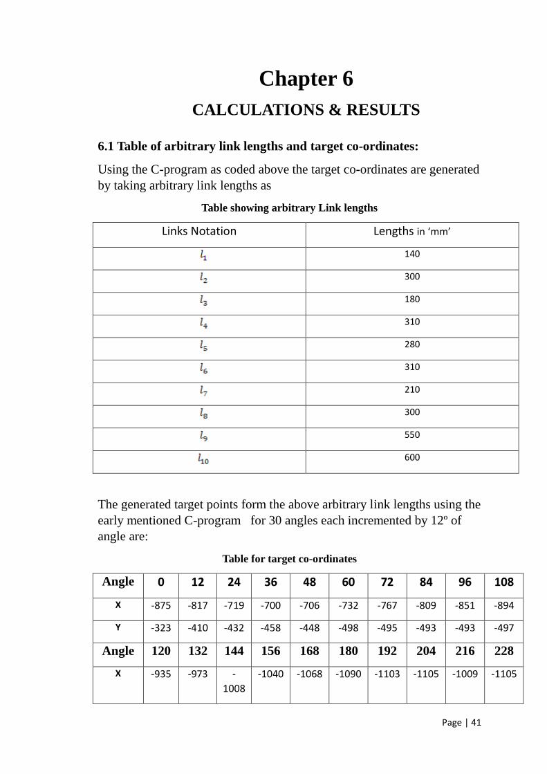
6.1 Table of arbitrary link lengths and target co-ordinates:

Using the C-program as coded above the target co-ordinates are generated

by taking arbitrary link lengths as

Table showing arbitrary Link lengths

Links Notation Lengths in ‘mm’

140

300

180

310

280

310

210

300

550

600

The generated target points form the above arbitrary link lengths using the

early mentioned C-program for 30 angles each incremented by 12º of

angle are:

Table for target co-ordinates

Angle 0 12 24 36 48 60 72 84 96 108

X -875 -817 -719 -700 -706 -732 -767 -809 -851 -894

Y -323 -410 -432 -458 -448 -498 -495 -493 -493 -497

Angle 120 132 144 156 168 180 192 204 216 228

X -935 -973 -

1008

-1040 -1068 -1090 -1103 -1105 -1009 -1105

Page | 42

Y -505 -516 -530 -542 -551 -553 -541 -498 -335 -169

Angle 240 252 264 276 288 300 312 324 336 348

X -

1082

-1046 -

1010

-985 -972 -969 -989 -963 -974 -900

Y 8.216 141 219 249 238 196 127 34 -61 -207

The locus generated by the above co-ordinates by keeping origin at the

crank is as:

AUTOCAD Drawing Showing target Path

6.2 Output of genetic algorithm:

Now to find out the link lengths by using the arbitrary values we have to

go through the modified GENETIC ALGORITHM

The modified genetic algorithm is executed by giving input as:

Total Number of Generations : 40

Page | 43

Population Size : 60

Cross Over Probability : 0.9

Mutation Probability : 0.0

Number of Variables : 10

Total Number of Runs : 5

Limits to Variables (Link Lengths) : 80 <= x1 <= 200

100 <= x2 <= 350

100 <= x3 <= 400

150 <= x4 <= 500

110 <= x5 <= 350

100 <= x6 <= 350

50 <= x7 <= 250

100 <= x8 <= 400

300 <= x9 <= 600

200 <= x10 <= 600

The Optimized output link lengths are generated with minimum fitness

0.00185 as:

Table for link lengths

Links Notation Generated Link Lengths

116.4

326.79

225.21

327.89

309.81

314.14

267.90

348.94

540.41

593.46

Page | 44

Form the above generated optimized link lengths the co-ordinates

of the generated locus are calculated.

6.3 Table comparing the target and generated co-ordinates

Crank Angle In Degrees

Target Path x, y Co-ordinates

Generated Path x, y Co-ordinates

Offset from

Target Distance in ‘mm’

0 (-875, -323) (-970, -179) 197.38

12 (-767, -410) (-939, -249) 235.5

24 (-719, -462) (-912, -303) 250

36 (-700, -488) (-895, -342) 243.6

48 (-706, -498) (-889, -369) 224

60 (-732, -498) (-895, -386) 198

72 (-767, -495) (-911, -411) 166.7

84 (-809, -493) (-933, -403) 153.2

96 (-851, -493) (-960, -408) 138

108 (-894, -497) (-990, -410.9) 129

120 (-935, -505) (-1020, -412) 126

132 (-973, -516) (-1050, -411) 130

144 (-1008, -530) (-1077, -406) 142

156 (-1040, -542) (-1102, -394) 160

168 (-1068, -551) (-1123, -372.66) 186.6

180 (-1090, -553) (-1140, -335) 223.66

192 (-1103, -541) (-1152, -277) 268.5

204 (-1105, -489) (-1158, -196) 297.75

216 (-1109, -355) (-1157, -94) 265.37

228 (-1105, -169) (-1145, 16) 189.2

240 (-1082, 8.216) (-1124, 117) 116.6

252 (-1046, 141) (-1098.7, 195) 75.45

264 (-1010, 219) (-1075, 241) 68.62

276 (-985, 249) (-1047, 240.66) 72.24

Page | 45

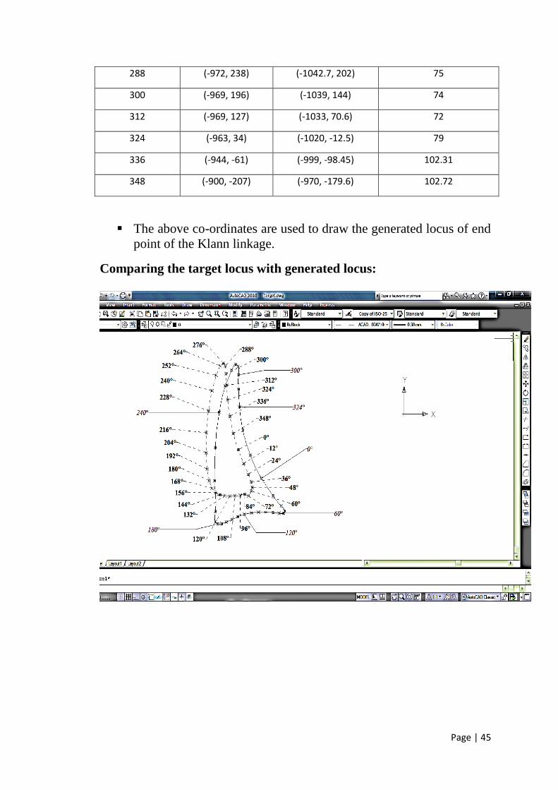
The above co-ordinates are used to draw the generated locus of end

point of the Klann linkage.

Comparing the target locus with generated locus:

288 (-972, 238) (-1042.7, 202) 75

300 (-969, 196) (-1039, 144) 74

312 (-969, 127) (-1033, 70.6) 72

324 (-963, 34) (-1020, -12.5) 79

336 (-944, -61) (-999, -98.45) 102.31

348 (-900, -207) (-970, -179.6) 102.72

Page | 46

Figure showing Comparision of Step Length And Step Height

From the above figure:

Desired Step Length =408.3mm

Desired Step Height =803.2mm

Generated Step Length=266.3mm

Generated Step Height=676.7mm

Page | 47

Chapter-7

CONCLUSION Conclusion In the present work we have consider a one-degree-of-freedom six-bar

linkage Klann linkage. The optimum link lengths for the desired locus is

calculated using genetic algorithm is also reported. The objective

function namely path error i.e. offset to all the precision points is

specified and tabulated.

From the above results the following conclusions are made

This thesis has succeeded in its objective of path synthesis of Klann

mechanism.

This thesis explains how the optimized link lengths of Klann

mechanism are derived using Genetic Algorithm for certain step

length and step height.

Even though we obtained the locus with optimized link lengths

there is a deviation of obtained locus from the desired locus due to

non-consideration of some of the constraints like mechanical

advantage of the linkage and flexibility effects can be also

considered to get the accuracy.

Future Scope:

As in hybrid synthesis approach the same linkage may be adopted for

both path synthesis and synthesis applications. The objective function

should be modified so as to get a different optimum link dimensions.

Finally, fabrication of the proto-type of linkage may be done to know the

difference between theoretically obtained end point co-ordinates and

actual values achieved.

Page | 48

Chapter-8

REFERENCES

1.Theory of Mechanisms and Machines by Amitabha Ghosh & Asok

Kumar Mallik

2. Introduction to Operations research by Frederick S.Hillier & Gerald

J.Liberman

3.http://www.mechanical spider.com

4. http://www.en.wikipedia.org/wiki/klann_linkage

5. http://www.friartuck.net/resources/optimization/what is

optimization.htm

6. http://www.robotronics09.blogspot.in/2011/01/klann-mechhanism.html

7. http://www.iitk.ac.in/kangal

8. http://www.mekanimalar.com/mechanicalspider .html

9. KLANN.J.C(2001).Patent No.6260862 United States

10. http://www.intechopen.com

11.Journal on KINEMATIC ANALYSIS AND SYNTHESIS OF AN

ADJUSTABLE 6-BAR LINKAGE by Gordon R.Pennock, Ali Israr

http://www.en.wikipedia.org/wiki/klann_linkage

http://www.friartuck.net/resources/optimization/what%20is%20optimization.htm

http://www.friartuck.net/resources/optimization/what%20is%20optimization.htm

http://www.robotronics09.blogspot.in/2011/01/klann-mechhanism.html

http://www.iitk.ac.in/kangal

http://www.mekanimalar.com/mechanicalspider%20.html

http://www.intechopen.com/

DESIGN AND OPTIMIZATION OF A ONE-DEGREE...

Documents

Transcript of DESIGN AND OPTIMIZATION OF A ONE-DEGREE...