DESIGN AND MANUFACTURING OF A QUAD TILT …etd.lib.metu.edu.tr/upload/12618110/index.pdf · ·...

DESIGN AND MANUFACTURING OF A QUAD TILT ROTOR

UNMANNED AIR VEHICLE

A THESIS SUBMITTED TO

THE GRADUATE SCHOOL OF NATURAL AND APPLIED SCIENCES

OF

MIDDLE EAST TECHNICAL UNIVERSITY

BY

AHMET CANER KAHVECİOĞLU

IN PARTIAL FULFILLMENT OF THE REQUIREMENTS

FOR

THE DEGREE OF MASTER OF SCIENCE

IN

AEROSPACE ENGINEERING

SEPTEMBER 2014

Approval of the thesis:



submitted by AHMET CANER KAHVECİOĞLU in partial fulfillment of the

requirements for the degree of Master of Science in Aerospace Engineering

Department, Middle East Technical University by,

Prof. Dr. Canan Özgen _____________________

Dean, Graduate School of Natural and Applied Sciences

Prof. Dr. Ozan Tekinalp _____________________

Head of Department, Aerospace Engineering

Prof. Dr. Nafız Alemdaroğlu _____________________

Supervisor, Aerospace Engineering Dept., METU

Examining Committee Members:

Prof. Dr. Serkan Özgen _____________________

Aerospace Engineering Dept., METU

Prof. Dr. Nafız Alemdaroğlu _____________________


Prof. Dr. Altan Kayran _____________________


Prof. Dr. Yusuf Özyörük _____________________


Prof. Dr. Kahraman Albayrak _____________________

Mechanical Engineering Dept., METU

Date: _________________

iv

I hereby declare that all information in this document has been obtained and

presented accordance with academic rules and ethical conduct. I also declare

that, as required by these rules and conduct, I have fully cited and referenced

all material and results that are not original to this work.

Name, Last name: Ahmet Caner KAHVECİOĞLU

Signature:

v

ABSTRACT



Kahvecioğlu, Ahmet Caner

M.S., Department of Aerospace Engineering

Supervisor: Prof. Dr. Nafiz Alemdaroğlu

September 2014, 145 pages

This thesis presents the design and manufacturing process of a mini class quad tilt

rotor unmanned air vehicle (UAV). An optimal design procedure is conducted to

satisfy a set of pre-determined requirements, which ensure a competitive aircraft

platform performing primarily intelligence, surveillance and reconnaissance missions

in UAV market.

The aircraft has four electric motors with tilting capability in one axis, which gives it

the opportunity to combine the vertical take-off and landing capabilities with long

endurance and good maximum cruise speed. In addition, as a result of the physical

concept and the modular design of the aircraft, wing and tail parts of the aircraft can

be demounted, so that the aircraft is converted to a highly maneuverable quad-rotor,

which has a longer hovering time capacity than the full aircraft and is more

appropriate for missions requiring stealth.

The thesis includes the construction of a mathematical model which calculates all of

the weight estimation parameters and geometrical and performance outputs;

generation of different design cases using this mathematical model and the procedure

for an optimal design choice; construction of the outer geometry and inner structure

vi

of the aircraft; manufacturing of the molds and the composite skins of the aircraft;

and assemblage of the aircraft. Outputs of the mathematical model are compared

with computational fluid dynamics (CFD) solutions to justify the analytical

calculations. Besides, static loading tests are conducted to examine the structural

design of the airframe.

The main objective of the study is to give an idea about the feasibility of developing

a new concept of a mini class UAV.

Keywords: Unmanned Air Vehicle, Tilt-rotor, Optimization, Design, Manufacture

vii

ÖZ

DÖRT DÖNER ROTORLU BİR İNSANSIZ HAVA ARACININ

TASARIM VE ÜRETİMİ

KAHVECİOĞLU, AHMET CANER

Yüksek Lisans, Havacılık ve Uzay Mühendisliği Bölümü

Tez Yöneticisi: Prof. Dr. Nafiz Alemdaroğlu

Eylül 2014, 145 sayfa

Bu tez, dört tilt rotorlu mini sınıf bir insansız hava aracının (İHA) tasarım ve üretim

sürecini konu almaktadır. Ağırlıklı olarak istihbarat, keşif ve gözlem görevlerini

yürütecek bu hava aracını İHA pazarında rekabet edebilir kılacak, önceden

belirlenmiş bir gereksinimler bütünü, optimal bir tasarım prosedürü uygulanarak

karşılanmaya çalışılmıştır.

Hava aracı dört adet tilt edilebilen- öne ve yukarı döndürülebilen- elektrik motoruna

sahiptir. Bu özelliği ona dikey iniş-kalkış imkânını, uzun uçuş süresi ve yüksek

azami seyir hızı yetenekleri ile birleştirme olanağı sunmuştur. Bunun yanında hava

aracının fiziksel konsepti ve modüler tasarımı, kanat ve kuyruk parçalarının

çıkarılarak; onun yüksek manevra kabiliyetli bir dört pervaneli helikoptere

dönüşmesini sağlar. Böylece hava aracı daha uzun bir dikey uçuş havada kalma

süresine sahip olur ve ayrıca dikkat çekmemesi gereken görevlere daha uygun hale

gelir.

Bu tez, tüm ağırlık tahmini, geometri ve performans parametrelerinin hesaplandığı

bir matematiksel modelin oluşturulması; bu model kullanılarak farklı tasarım

alternatiflerinin oluşturulması ve optimum tasarım tercihinin yapılmasına dair

viii

yöntem; uçağın dış geometrisi ve iç yapısının oluşturulması; uçağın kalıpların ve

kompozit yüzeylerinin üretilmesi ve uçağın montajı konularını kapsamaktadır.

Matematiksel modelden alınan sonuçlar, hesaplamalı akışkanlar dinamiği (HAD)

çözümlerinden alınan veriler ile kıyaslanmış ve analitik hesaplar doğrulanmıştır.

Hava aracının yapısal tasarımı, uygulanan statik yükleme testleri ile kontrol

edilmiştir.

Bu çalışmanın temel amacı yeni bir konsepte sahip, mini sınıf bir İHA’nın

geliştirilmesinin yapılabilirliği hakkında fikir vermektedir.

Anahtar Kelimeler: İnsansız Hava Aracı, Tilt-rotor, Optimizasyon, Tasarım, Üretim

ix

To Olric…

x

ACKNOWLEDGMENTS

I am grateful to my supervisor Prof. Dr. Nafız Alemdaroğlu due to his support,

advice and encouragements through my thesis work. I would like to thank Prof. Dr.

Altan Kayran for his help in manufacturing process. I also want to thank Mr. Ender

Özyetiş and Mr. Güçlü Özcan for their help in the testing phase. Besides I am very

grateful to my family for their support and encouragements.

xi

TABLE OF CONTENTS

ABSTRACT ............................................................................................................. v

ÖZ ......................................................................................................................... vii

ACKNOWLEDGMENTS ....................................................................................... x

TABLE OF CONTENTS ....................................................................................... xi

LIST OF TABLES ................................................................................................. xv

LIST OF FIGURES ............................................................................................. xvi

1. INTRODUCTION ........................................................................................... 1

1.1 The Concept of Tilt Rotor ......................................................................... 2

1.2 The Concept of Convertible Mini Quad Tilt Rotor UAV ......................... 2

1.3 The Design Philosophy ............................................................................. 5

1.4 Literature Survey ....................................................................................... 6

Competitor Study ................................................................................................. 9

1.5 Determination of Requirements .............................................................. 11

Mission Profile ................................................................................................... 11

Cruise Speed ...................................................................................................... 13

Payload ............................................................................................................... 13

Operational Altitude ........................................................................................... 13

Weight ................................................................................................................ 14

Stall Speed .......................................................................................................... 14

Wing Span .......................................................................................................... 14

Power Unit ......................................................................................................... 14

Endurance ........................................................................................................... 14

2. CONCEPTUAL DESIGN PROCEDURE ..................................................... 17

xii

2.1 Structure of MS Excel and Ansys Workbench Design Exploration Toolbox

Coupled Design Study ........................................................................................... 17

2.2 Construction of the MS Excel File ......................................................... 19

Input Parameters ................................................................................................. 20

Weight Estimation Parameters ........................................................................... 26

Drag Estimation Parameters ............................................................................... 33

Geometrical Output Parameters ......................................................................... 34

Performance Output Parameters ......................................................................... 36

2.3 Determination of Inputs, Outputs and Optimization Criteria ................. 40

2.4 Procedure in Ansys Workbench Design Exploration Toolbox .............. 45

Design of Experiments ....................................................................................... 45

Response Surface ............................................................................................... 47

Optimization ....................................................................................................... 48

3. OUTCOME OF THE OPTIMIZATION AND DECISION OF THE FINAL

CONFIGURATION .............................................................................................. 49

3.1 Important Correlations and Graphs ........................................................ 49

Local Sensitivities .............................................................................................. 49

Response Curves ................................................................................................ 51

Trade off Charts ................................................................................................. 59

3.2 The Decision of the Final Design ........................................................... 63

3.3 The Numerical Outputs .......................................................................... 67

Geometrical Outputs .......................................................................................... 67

Weight Outputs .................................................................................................. 68

Aerodynamic and Performance Outputs ............................................................ 68

3.4 Constructing the Outer Geometry........................................................... 71

Fuselage .............................................................................................................. 71

xiii

Wing ................................................................................................................... 72

Booms ................................................................................................................ 72

Tails .................................................................................................................... 72

3.5 Structure of the Components and Inner Placement ................................. 75

Fuselage.............................................................................................................. 75

Wing ................................................................................................................... 76

Horizontal and Vertical Tails ............................................................................. 77

Placement inside the Fuselage ........................................................................... 78

3.6 Static Margin Calculation ........................................................................ 79

4. MANUFACTURING ..................................................................................... 83

4.1 Constructing a Manufacturable Geometry .............................................. 83

Carrying the Numerical Values of the Design Output to the CAD ................... 83

Splitting the Geometry and Drawing the Female Molds ................................... 85

4.2 Manufacturing of the Molds .................................................................... 88

Defining the Tool-paths and Generating the Numerical Code........................... 88

Machining the Molds ......................................................................................... 88

Surface Finish Treatments.................................................................................. 90

4.3 Manufacturing of the Composite Skins and Inner Structural Frames ..... 91

Methodology ...................................................................................................... 91

Fuselage.............................................................................................................. 92

Wing and Tail ..................................................................................................... 94

Inner Structural Frames ...................................................................................... 95

Weights of the Produced Parts ........................................................................... 96

4.4 Assemblage ............................................................................................. 96

Fuselage.............................................................................................................. 96

Wing ................................................................................................................... 98

xiv

Tails .................................................................................................................. 100

Weights of the Assembled Parts ....................................................................... 102

Preparation of the Aircraft for Future Work .................................................... 105

5. CONCLUSION ........................................................................................... 109

REFERENCES .................................................................................................... 113

APPENDICIES ................................................................................................... 119

A.COST ANALYSIS .......................................................................................... 119

B.MOTOR DATASHEET .................................................................................. 121

C.JUSTIFICATION OF AERODYNAMICAL OUTPUTS BY CFD

CALCULATIONS .............................................................................................. 123

D.CONCEPTUAL PROBLEM: DRAG FORCE ON MOTOR BOOMS .......... 131

E.JUSTIFICATION OF THE STRUCTURAL DESIGN OF THE AIRCRAFT BY

STATIC LOADING ............................................................................................ 141

xv

LIST OF TABLES

Table 1.1Competitor Study ........................................................................................ 10

Table 2.1 Airfoil Comparison @ Re=200000 [41] .................................................... 23

Table 2.2 Defined Parameters in Optimization Toolbox and Optimization Criteria . 44

Table 2.3 Output of Design of Experiments .............................................................. 46

Table 2.4 Goodness of Fit Table ................................................................................ 47

Table 3.1 Geometrical Outputs .................................................................................. 67

Table 3.2 Weight Outputs .......................................................................................... 68

Table 3.3 Aerodynamic and Performance Outputs .................................................... 68

Table 3.4 Weight Distribution of the Fixed Wing Mode ........................................... 80

Table 4.1 Comparison of the Calculated and Measured Weights of the Composite

Skin Parts ................................................................................................................... 96

Table 4.2 Comparison of the Calculated and Measured Weights of the Assembled

Parts .......................................................................................................................... 103

Table A.1 Costs of the Components ........................................................................ 119

Table B.1Performance of the Motor with Different Propellers ............................... 121

Table C.1 Drag Force Comparison of CFD Results with Analytical Calculations .. 128

Table D.1 Drag Forces on Components at 20 m/s with zero angle of attack ........... 131

Table E.1 Loads at the Stations in 1g Static Wing Loading Test ............................ 142

Table E.2 Loads at the Stations in 3g Static Wing Loading Test ............................ 143

xvi

LIST OF FIGURES

Figure 1.1Conceptual Sketch of the Aircraft (Quad-rotor Mode) ................................ 3

Figure 1.2 Conceptual Sketch of the Aircraft (Fixed Wing Mode) ............................. 4

Figure 1.3 Flow-field of Tilting Rotors Mounted on the Wing (Out of Ground Effect)

(from [3]) ...................................................................................................................... 4

Figure 1.4 Flow-field of Tilting Rotors Mounted on the Wing (In Ground Effect)

(from [3]) ...................................................................................................................... 5

Figure 1.5Schematic of the Conceptual Design Methodology .................................... 6

Figure 1.6 Experimental Prototype in [15] (from [15]) ............................................... 7

Figure 1.7 AeroVironment Shrike ................................................................................ 8

Figure 1.8IAI Ghost ..................................................................................................... 8

Figure 1.9IAI Mini Panther .......................................................................................... 9

Figure 1.10IAI Bird Eye 500 ........................................................................................ 9

Figure 1.11Primary Mission Profile (Mission 4) ....................................................... 13

Figure 2.1Flowchart of the Optimization Procedure (Green and Yellow Blocks are

Excel and Ansys Part Respectively) ........................................................................... 17

Figure 2.2Analysis and Project Schematics in Ansys Workbench ............................ 18

Figure 2.3Defining Objectives and Constraints in the Optimization Section ............ 19

Figure 2.4Scheme of MS Excel File .......................................................................... 20

Figure 2.5Polars of SD7062 @Re=200000[41] ......................................................... 23

Figure 2.6Fuselage Skin Plies (without -on the left hand side- and with reinforcement

-on the right hand side-) ............................................................................................. 27

Figure 2.7Wing Skin Plies (without -on the left hand side- and with reinforcement -

on the right hand side-) ............................................................................................... 28

Figure 2.8Horizontal and Vertical Tail Skins Plies (without -on the left hand side-

and with reinforcement -on the right hand side-) ....................................................... 28

xvii

Figure 2.9Defined Parameters in Excel Interface of Ansys Workbench ................... 40

Figure 2.10The Procedure in Design of Experiments Phase ..................................... 45

Figure 2.11 Accuracy of Response Surface ............................................................... 48

Figure 3.1Local Sensitivity Bars @W/S=140, AR_wing=9.5, V=20m/s .................. 50

Figure 3.2W/S and AR_wing Response of ENDURANCE_4 @V=20 m/s .............. 52

Figure 3.3Wing Loading and Wing Aspect Ratio Responses of ENDURANCE_4

@V=25m/s ................................................................................................................. 52

Figure 3.4Velocity Response of ENDURANCE_4 @W/S=140 N/m2, AR_wing=9,5

.................................................................................................................................... 53

Figure 3.5Wing Aspect Ratio Response of Design Take-off Weight @W/S=140

N/m2, V=20 ................................................................................................................ 54

Figure 3.6Wing Loading Response of Design Takeoff Weight @AR_wing=9.5,

V=20m/s ..................................................................................................................... 54

Figure 3.7 Wing Loading Response of Stall Speed @AR_wing=9.5, V=20m/s ....... 55

Figure 3.8 Wing Loading and Wing Aspect Ratio Responses of ENDURANCE_1

@V=20m/s ................................................................................................................. 56

Figure 3.9Velocity Response of ENDURANCE_1@W/S=140 N/m2, AR_wing =9.5

.................................................................................................................................... 57

Figure 3.10 Wing Loading and Wing Aspect Ratio Response of ENDURANCE_2 58

Figure 3.11 Wing Loading and Wing Aspect Ratio Response of ENDURANCE_3 58

Figure 3.12 Wing Loading and Wing Aspect Ratio Response of Wing Span .......... 59

Figure 3.13 Trade-off Between W/S and AR_wing................................................... 60

Figure 3.14 Trade-off between W_0 and ENDURANCE_4 .................................... 61

Figure 3.15 Trade-off Between Stall Speed and ENDURANCE_4 .......................... 61

Figure 3.16 Trade-off Between Stall Speed and W_0 ............................................... 62

Figure 3.17Trade-off Between The Wing Span and Aspect Ratio ............................ 62

Figure 3.18The candidate Points ................................................................................ 63

xviii

Figure 3.19ENDURANCE_4 Values of the Candidates (units are in minutes) ......... 64

Figure 3.20Design Take-off Weight Values of the Candidates (units are in grams) . 64

Figure 3.21Stall Speed Values of the Candidates (units are in m/s) .......................... 65

Figure 3.22Wing Span Values of the Candidates (units are in meters) ..................... 65



Figure 3.25Variation of Maximum Load Factor with Velocity ................................. 70

Figure 3.26 Variation of Power Required and Power Available with Velocity ......... 70

3.27Rate of Climb Variation with Velocity ............................................................... 71

Figure 3.28Isometric View of the Quad-rotor Mode of the Aircraft ......................... 73

Figure 3.29Isometric View of the Fixed Wing Mode of the Aircraft (Horizontal

Flight Mode) ............................................................................................................... 73

Figure 3.30 Isometric View of the Fixed Wing Mode of the Aircraft (Vertical Flight

Mode) ......................................................................................................................... 74

Figure 3.31The Front, Top and Right Views of the Fixed Wing Mode of the Aircraft

.................................................................................................................................... 75

Figure 3.32Inner Structure of the Fuselage ................................................................ 76

Figure 3.33Inner Structure of the Wing ..................................................................... 77

Figure 3.34Inner Structure of the Horizontal Tail ...................................................... 77

Figure 3.35Inner Structure of the Vertical Tail .......................................................... 78

Figure 3.36 Placement of the Components (Fixed Wing Mode) ............................... 79

Figure 3.37 Placement of the Components (Quad-rotor Mode) ................................. 79

Figure 4.1Construction of the Wing Surface ............................................................. 83

Figure 4.2Manufacturing Steps .................................................................................. 84

Figure 4.3Guiding Curves and Reference Cross-Sections of the Fuselage ................ 85

Figure 4.4 An Example of Adverse Slope on Molds ................................................. 86

Figure 4.5 CAD Drawing of the Molds (one side only) ............................................. 87

xix

Figure 4.6 An Example of Tool-Paths (Left Wing Lower Surface Finishing Tool-

Path) ........................................................................................................................... 88

Figure 4.7 Machining the Fuselage Mold .................................................................. 89

Figure 4.8 Scenes from Machining of the Molds (Finishing of the wing and

horizontal tail; roughening of the vertical tail) .......................................................... 89

Figure 4.9 Scenes from Surface Finishing Treatments (Polyester putty on fuselage

mold, applying primer on wing molds and varnished molds) .................................... 90

Figure 4.10 Vacuum Bagging Wet Lay-up Method (from [51]) ............................... 92

Figure 4.11Manufacturing of the Fuselage Skins ...................................................... 93

Figure 4.12Manufacturing of the Wing Skins............................................................ 94

Figure 4.13 All of the Composite Skins Parts of the Aircraft .................................... 95

Figure 4.14 Manufacturing of the Inner Structural Frames ....................................... 95

Figure 4.15Assemblage Steps of the Fuselage ........................................................... 97

Figure 4.16 Assembled Fuselage ............................................................................... 98

Figure 4.17 Front Spar of the Wing ........................................................................... 98

Figure 4.18Preparing the Upper Wing Surface .......................................................... 99

Figure 4.19Assembled Wings .................................................................................... 99

Figure 4.20 Inner Structure of the Tail Surfaces ...................................................... 100

Figure 4.21 Horizontal Tail Adhered to the End of the Tail Boom ......................... 100

Figure 4.22Positioning and Adhering the Vertical Tail ........................................... 101

Figure 4.23Assembled Horizontal and Vertical Tails .............................................. 101

Figure 4.24Views of the Assembled Aircraft .......................................................... 104

Figure 4.25 Electronic Equipment and Cabling Installed on the Prototype ............. 105

Figure 4.26RadioReceiver, Flight Controller, Servo Multiplexer Card and Cabling

Installed on the Aircraft ........................................................................................... 106

Figure 4.27 Tilt Mechanism Installed on the Aircraft .............................................. 106

Figure 4.28 View of the Equipped Aircraft (Fixed Wing Mode)for R/C Flight ...... 107

xx

Figure 4.29 View of the Equipped Aircraft (in Quad-rotor mode) for R/C Flight .. 107

Figure 4.30 A Scene From Vertical Flight in Quad-rotor Mode .............................. 108

Figure C.0.1Boundary Mesh on the Wall Surfaces .................................................. 124

Figure C.0.2 Computational Domain ....................................................................... 124

Figure C.0.3 Cross-section of the motor boom in computational mesh ................... 125

Figure C.0.4Lift Coefficient Variation of the Full Aircraft with Angle of Attack .. 125

Figure C.0.5 Drag Coefficient Variation of the Full Aircraft with Angle of Attack 126

Figure C.0.6Static Pressure Contours at 20 m/s and Zero Angle of Attack ............. 127

Figure C.0.7 Body-y Moment Coefficient Variation of the Full Aircraft with Angle

of Attack (In Stability Axes [56]) ............................................................................ 129

Figure C.0.8Body-z Moment Coefficient Variation of the Full Aircraft with Angle of

Attack (In Stability Axes [56]) ................................................................................. 129

Figure C.0.9 Static Pressure Contours at 20 m/s and 10° Side-slip Angle .............. 130

Figure D.0.1Velocity Vectors around the Motor Boom at 20 m/s with zero angle of

attack ........................................................................................................................ 132

Figure D.0.2 Static Pressure Contours around the Motor Boom at 20 m/s with zero

angle of attack .......................................................................................................... 132

Figure D.0.3 Static Pressure Contours of the Aircraft Version without Motor Booms

at 20 m/s with zero angle of attack ........................................................................... 133

Figure D.0.4Separation Points on several 2-d elliptical and Jukowsky shapes

determined by theoretical analysis of the boundary layer flow (from [45]) ............ 133

Figure D.0.5 A Possible Tilting-Fairing Solution to Reduce the Form Drag (Upper

configuration in horizontal flight and lower configuration in hovering) ................. 134

Figure D.0.6 Delay Separation on Golf Ball (from [57]) ........................................ 135

Figure D.0.7The Mechanism of Flow Separation Delaying by Dimples on Surface

(from [58]) ................................................................................................................ 135

Figure D.0.8 Drag Coefficient Variation of Some Geometries with Reynolds

Number ([from[58]) ................................................................................................. 136

xxi

Figure D.0.9 Sketch of the Experimental Flow Geometry [59] (from [59]) ............ 136

Figure D.0.10Flow Visualization of the Experiment in [59] (from [59]) ................ 137

Figure D.0.11 Influence of Splitter Plates on Drag Coefficients of Several

Geometries (from [45]) ............................................................................................ 138

Figure D.0.12Effects of Splitter Plates upon Stv and Localised Pressure Coefficient

(from [61]) ................................................................................................................ 139

Figure E.0.1 1g Static Wing Loading Test (about 2.5kg at each wing) ................... 141

Figure E. 0.2 1g Static Wing Loading Test (about 2.5kg at each wing) .................. 142

Figure E. 0.3 Wing Deformation in 1g Static Wing Loading Test .......................... 143

Figure E.0.4 3g Static Wing Loading Test (about 7.5 kg at each wing) .................. 144

Figure E.0.5 Wing Deformation in 1g Static Wing Loading Test ........................... 144

Figure E.0.6Static Loading of Motor Booms ........................................................... 145

1

CHAPTER 1

1. INTRODUCTION

The zeitgeist of the moment gives prominence to the unmanned air vehicles (UAV’s)

in many areas of aviation. Countless applications have been realized so far, and many

others still have their potentials. Lower manufacturing and operation costs and more

flexible mission profiles due to the absence of pilot make UAV’s more preferable in

many military and civil applications. In macro scale, there is a trend to replace the

manned air vehicles with UAV’s having the same mission profiles. Similarly, in

smaller scales, autonomous controls take the place of the remotely piloting and

eliminate many handicaps like hardship of performing some manoeuvres or human

fatigue. In addition to this, small scale aircraft have started to become important in

completely new military and civil areas by means of developing hardware and

software technologies.

As the application areas expand, new requirements arise. For the last few decades,

the micro and mini class UAV’s have not been seen as remotely piloted hobby toys.

They have become today’s most versatile vehicles for surveillance, mapping, target

tracing and search-rescue operations. In addition to that other missions including

target demolishing, electronic warfare and establishing data link are done by small

UAV’s. One of the most important factor for small scale UAV’s to have a wide

operation spectrum is their low manufacturing and operating cost. For many

operations, they are considered as disposable or expendable.

Many small scale UAV’s are used as a part of a man portable system on the field. As

they are carried by men, these systems are light-weight and less complicated. Also,

these aircraft generally do not need runway to take-off. Some of them have VTOL

capabilities; and the others are launched by hand or by using catapults. For recovery,

some of the ones without VTOL capabilities use parachute or airbag; or both. Other

2

methods like belly landing, deep stall, catching by a net or hook are also used in

these systems.

1.1 The Concept of Tilt Rotor

The tilt rotor concept is a combination of horizontal flight of a fixed wing and VTOL

capabilities of a rotary wing. It has good endurance and forward velocity properties

while it does not need a runway. At the instances of take-off and landing, the axes of

the rotors are perpendicular to the ground; and parallel during the horizontal flight.

The rotors are tilted when transition between vertical and horizontal flights is

performed.

In general, for all scales the most obvious advantage of the tilt rotor concept is to

eliminate the need for a runway. For mini class UAV’s, it may be thought that it is

unnecessary to add complication for that feature; as they already do not need runway.

On the other hand, firstly for take-off many of these systems include catapults, which

have a certain weight. Secondly, in many operations precision of the landing point is

very important. Parachute recovery may have problem with that issue in case of

windy weathers. Belly landing and catching by net are more difficult methods to

perform, including the risk of damaging the aircraft.

A mini class rotary wing UAV has other problems. Firstly, rotary wings are more

fragile to the wind conditions. Their flight conditions are more limited with respect

to the fixed wing aircraft. In addition to that, their forward speed is significantly

lower than fixed wings. Also their endurances are very low comparing with the fixed

UAV’s.

Apart from those, tilt rotor concept brings completely different operational

capabilities to a fixed wing aircraft. Mode transition from horizontal flight to

hovering during mission becomes possible, which is very critical for reconnaissance

operations.

1.2 The Concept of Convertible Mini Quad Tilt Rotor UAV

The subject of this study is a mini class quad tilt rotor UAV, whose tail and wing can

be demounted optionally. When its tail and wing are demounted, the aircraft

becomes a highly manoeuvrable quad-rotor with same payload. There are two

3

advantages of this: Firstly the aircraft gets rid of the weights of the tail and wing; and

an extra battery can be loaded instead. So a significant increase in endurance is

obtained. Secondly, for some special missions where stealth is an issue, the aircraft

gets rid of its long wing and tail; and for search and rescue operations, it enables the

aircraft to enter some narrower spaces like inside of a building or a cave. Briefly,

these are the main motivations for developing this aircraft concept. In addition to

enhancing the operational capabilities, charging battery from the electric poles may

be possible with new technological developments in battery technologies in future.

Such a development would make this concept very advantageous in the market.

The quad-rotor mode and the fixed wing mode of the aircraft are shown in Figure 1.1

and Figure 1.2 respectively.

Figure 1.1Conceptual Sketch of the Aircraft (Quad-rotor Mode)

4

Figure 1.2 Conceptual Sketch of the Aircraft (Fixed Wing Mode)

A tandem wing configuration, where the tilting rotors are mounted on the wings, like

the other QTR’s [1], [2] is not chosen for some reasons. Although it may turn into an

advantage in ground effect condition; the rotor wake towards the upper wing surface

causes a high download force, which decreases the aircraft’s lifting capacity out of

ground effect [3]. The situation is shown in Figure 1.3 and Figure 1.4.

Figure 1.3 Flow-field of Tilting Rotors Mounted on the Wing (Out of Ground Effect) (from [3])

Wing

Rotor

5

Figure 1.4 Flow-field of Tilting Rotors Mounted on the Wing (In Ground Effect) (from [3])

In this study’s concept, instead of the wing upper surface, only boom sees the rotor

wake. So during the vertical flight download due to the rotor wake is reduced. On the

other hand, as a weakness of this study’s concept, in horizontal flight, motor booms

directly see the free stream, which increases the drag dramatically. This issue is

discussed in APPENDIX D.

Another option to prevent this adverse effect is to use a ducted fan. However, the

ducts themselves create significant drag and in addition to this the ducts increase the

weight of the aircraft. [4]

This aircraft concept is genuine with its option to convert tilt rotor aircraft into quad-

rotor. By demounting the wing and the tail, not only the weight is decreased, but also

the manoeuvrability is enhanced by decreasing the moment of inertias of the aircraft

significantly.

1.3 The Design Philosophy

A design study is making a chain of decisions to create something acceptable for

requirements. Generally there are many ways to reach a goal. Moreover, some of

these ways may also contain decisions without good reasoning. On the other hand,

some initial decisions and acceptances without good reasoning may lead non-optimal

solutions. The very basic notion behind this design study is that good reasoning is

tried to be made for every single design choice. Therefore, a multi-objective

optimization tool is used at the conceptual design level.

6

Only empirical formulas are used to conduct the iterative calculations, but no CFD or

FEM analyses data is used in conceptual design phase considering the calculation

costs.

As the study includes manufacturing, any unrealistic result may affect the credibility

of the whole study. So, manufacturability is always considered in decisions.

In practice, a mathematical model, which is specific for this concept, is constructed

in MS EXCEL. In this model, structural and aerodynamic calculations are conducted

iteratively. In Ansys Workbench’s Design Optimization Toolbox, desired

requirements and objectives are defined and let the toolbox choose the best

combinations of design choices by using the MS EXCEL as solver.

1.4 Literature Survey

In large scale, The Bell Boeing V-22 Osprey [5] is the most known example of the

tilt rotor concept. It is a manned aircraft and widely used in military operations. A

smaller version of V-22, The AW609 [6] is another manned tilt rotor aircraft mainly

used in civil operations. These two aircraft have two rotors having swash blades and

hinge mechanisms [4]. The Bell X-22 can be shown as an example of manned quad

tilt rotor aircraft, whose program was cancelled in late 80’s. [1] Today “Bell Boeing

Quad Tilt Rotor” [2], which is C-130 sized cargo aircraft, is an on-going project.

REQUIREMENTS

MS EXCEL

(MATHEMATICAL MODEL)

ANSYS WORKBENCH

OPTIMIZATON TOOLBOX

OUTPUT

Figure 1.5Schematic of the Conceptual Design Methodology

7

Boeing Phantom Swift [7] is another on-going tilt rotor project. It shows that the tilt

rotor concept is still alive in large scale.

The Bell Eagle Eye [8], IAI Panther [9] and KARI Smart UAV [10] are mid-scale

UAV’s. TURAC [11], which is a tilt rotor with three motors, is also an on-going

project from Turkey. Koker 1 [12] is another quad tilt wing developed in Iran having

similar scales.

In small scale, there are many VTOL aircraft in market, which are mainly helicopters

and multi-copters. Only IAI Mini Panther [13] is a tilt rotor UAV, which is the

closest concept for this study. In academic side, in recent years, SUAVI, which is a

tilt wing UAV, is developed in small scales [14]. In addition, the aircraft mentioned

in [15] has the same physical concept to this study. In [15], the modelling and control

aspects of this concept are examined.

Figure 1.6 Experimental Prototype in [15] (from [15])

Interest on this subject is very extensive nowadays. There are also many individual

developers in VTOL aircraft area. The most of these individual efforts are on small

scales. However, these valuable works are mostly remotely piloted aircraft with no

payload; and their specifications are not available. So, they cannot be considered in

competitor study. On the other hand, the fixed wing aircraft in same class are taken

into account in competitor study, as they have similar mission profiles.

8

In competitor study, numerous aircraft with same objectives are examined, and some

of them are listed. Besides, some of them are more important than other, which shape

the concept of the aircraft.

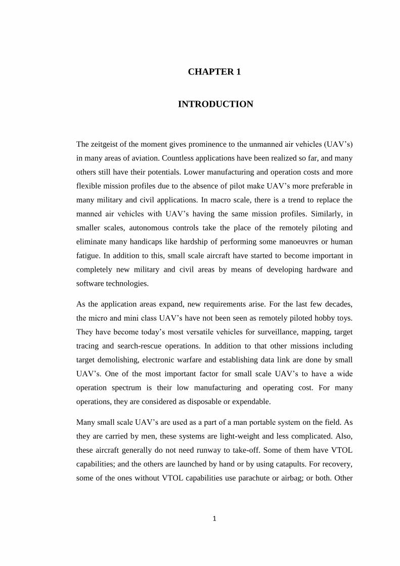
AeroVironment SHRIKE: This is a quad-rotor with a camera as payload. It answers

the need of stealth UAV capable of perching and staring. [16] Shrike has a very good

endurance. It is ideal for intelligence operations. It is small enough to be carried in a

backpack.

Figure 1.7 AeroVironment Shrike

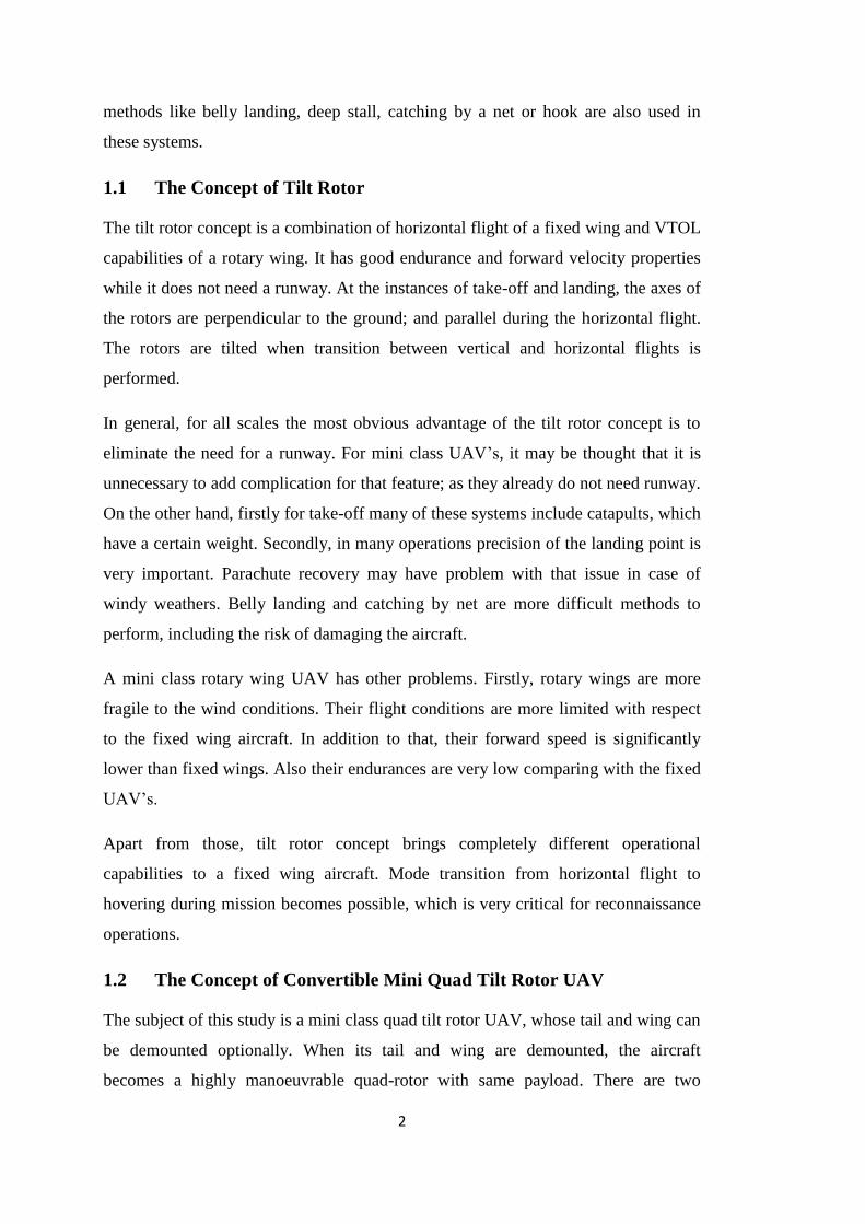
IAI GHOST: It is another stealthy UAV that can operate day and night. It also has

good endurance. It is especially optimized to operate in urban areas. [17] It has twin

rotor configuration and it is a very stable aircraft even in case of side-winds and

gusts.

Figure 1.8IAI Ghost

9

IAI MINI PANTHER: It is a tilt rotor with three electric motors. It has a wide range

of mission capabilities combining the bests of rotary wing and fixed wing concepts

[13]. Despite of being slightly larger, it is the closest aircraft to this study’s concept

in UAV market.

Figure 1.9IAI Mini Panther

IAI BIRD-EYE 500: As a fixed wing aircraft, the physical properties are expected to

be very similar with this aircraft. It is again used mainly in intelligence, surveillance,

reconnaissance (ISR) missions. The whole system including two aircraft, one ground

control station (GCS) is carried in two backpacks and operated by two unskilled

soldiers. [18] It is launched by hand or bungee.

Figure 1.10IAI Bird Eye 500

Competitor Study

Some important aircraft having similar objectives are listed. Except RQ-16 T-Hawk,

which has piston motor, all of the competitors have electric driven motors. Some of

the data of the aircraft are missing and could not be found in literature.

10

Table 1.1Competitor Study

COMPETITOR CONCEPT MTOW SPAN LENGTH OPRT. RANGE

ENDURANCE

CRUISE SPEED

PAYLOAD WEIGHT

OPRT. ALTITUDE

Raven (RQ-11B) [19]

Fixed Wing

1.9 kg 1.3 m

1.09 m 10 km 60-90 min

16 m/s - -

Puma (RQ -20) [20]

Fixed Wing

5.9 kg 2.8 m

1.4 m 15 km 120 min 10-23 m/s

- -

EMT Aladin[21] Fixed Wing

3.2 kg 1.46

m 1.53 m

> 15 km

30-60 min

45-90 m/s

- -

Orbiter[22] Fixed Wing

6.5 kg 2.2 m

1 m 15 km 120-180

min 10-38 m/s

- 5500 m

Skylite B[23] Fixed Wing

6 kg 2.4 m

1.15 m 10 km > 90 min 20-33 m/s

750 gr 100-600 m (AGL)

Bird-Eye 400[24]

Fixed Wing

5.6 kg 2.2 m

0.8 m 10 -15

km 60 min

15-25 m/s

1.2 kg 1000 m (AGL)

Bird-Eye 500[18]

Fixed Wing

5 kg 2 m 1.6 m 10 km 60 min 10-30 m/s

850 gr 500 m (AGL)

Casper 200[25] Fixed Wing

2.3 kg 2 m 1.3 m 10 km 90 min 10-25 m/s

240 gr 250 m (AGL)

DP-6 Whisperer[26]

Tandem Helicopter 23 kg 2m 2m 80 km

60-30 min

35 m/s 1-7kg 5000 m

Ghost[17] Tandem

Helicopter 4 kg -

0.75 x 1.45 m

- 30 min 0-18 m/s

600 gr Dozens

of meters

Shrike[16] Quadrotor 2.5 kg N/A - 5 km 40 min 15 m/s - -

HeliSpy II[27] VTOL 2 kg 0.28

m 0.7 m - -

> 34 m/s

- -

Datron Scout[28]

Quadrotor 1.3 kg N/A 0.8

x.08 x 0.2 m

3 km 20 min 14 m/s - 500 m (AGL)

RQ-16 T-Hawk[29]

Ducted Fan VTOL

8.4 kg N/A - 11 km 40 min 36 m/s - 3200 m

Oviwun[30] Ducted

Fan VTOL 2.5 kg

64.7 cm

41.1 cm

1.6 km 20 min 14 m/s 0.5-3 kg 5875 m

Mini Panther [13]

Tilt Rotor 12 kg 3.2 m

- 20 km 90 min 20 m/s 2 kg 1500 m (AGL)

Turac [11] Tilt Rotor 47 kg 4.2 m

1.8 m - 85 min 20 m/s 8 kg -

All the competitors carry optical sensors in normal, and they are mainly used for

reconnaissance and surveillance missions. However, none of them is so similar to

11

this study’s concept; so that the requirements of the aircraft for being a competitive

option cannot be determined directly. Moreover, the numbers may not show

everything and some qualitative properties can make an aircraft preferable. Therefore

some basic requirements are accepted as is; and some of them are used to get an idea.

First of all, the payload and data-video links are roughly determined by the

competitor study only. These kinds of aircraft stream video up to 15 km, and the

gimbal-optical sensor combination has some standards. So these are going to be

determined accordingly. So even without knowing exactly which cameras are used in

those aircraft, it can be said that the payload to be chosen is going to weigh around

these values.

The weights and the sizes of the aircraft vary in a range. The average values are

taken into account.

The endurance values give a rough idea. The fixed wing aircraft have endurances

above one hour. The rotary wing aircraft have endurances up to 40 minutes, except

DP-6 Whisperer, which is a relatively larger scale aircraft.

All the candidates use electric motors. This choice is somehow obvious for this scale

considering the acoustic emission and maintenance issues.

Last but not least, the cruise speed is going to be determined considering these

numbers. The cruise speed should be a reason for preference for choosing this

concept instead of a rotary wing.

1.5 Determination of Requirements

Mission Profile

There are some mission profile options determined for this aircraft. These are:

- Horizontal Flight Fixed Wing Mode (MISSION 1)

- Vertical Flight in Fixed Wing Mode (MISSION 2)

- Vertical Flight in Quad-Rotor Mode (MISSION 3)

- Combined Flight in Fixed Wing Mode (MISSION 4)

12

These mission profiles are represented by some formulas in prepared MS Excel file.

Their endurance values are calculated and parameterized in optimization phase.

The horizontal flight in fixed wing mode refers the mission including:

i. Vertical Take-Off for 15 seconds with a vertical velocity about 1 m/s

ii. Transition to horizontal flight mode (rotors are perpendicular to the ground) and

climb to the operational altitude

iii. Loiter

iv. Descend and transition to vertical flight mode (rotors are parallel to the ground)

v. Vertical Landing for 15 seconds with a vertical velocity about 1 m/s

The vertical flight in fixed wing and quad-rotor modes refer the same mission

profile, but in different modes:

i. Vertical Take-Off for 15 seconds with a vertical velocity about 1 m/s

ii. Vertical Flight to operation zone, execute the mission

iii. Vertical Landing for 15 seconds with a vertical velocity about 1 m/s

The combined flight in fixed wing mode is the primary mission profile, and the

endurance of this mission profile is going to be maximized during the optimization

based design procedure.

i. Vertical Take-Off for 15 second with a vertical velocity about 1 m/s

ii. Transition to horizontal flight mode and climb to the operational altitude

iii. Loiter

iv. Transition to vertical flight mode, hovering above the target for 5 min and

collecting detailed data

v. Transition to horizontal flight mode and loiter

vi. Descend and transition to vertical flight mode

vii. Vertical Landing for 15 seconds with a vertical velocity about 1 m/s

13

Cruise Speed

The cruise speed should be an advantage over the rotary wing aircraft. So design

cruise speed should not be too low. On the other hand, increasing the cruise velocity

dramatically decreases the endurance. Looking at the competitor study ([11], [13],

[23]) a design cruise speed of 20 m/s is determined to be a good compromise.

Payload

Payload is a gimbal with optical sensors. For the design procedure, only physical

properties of the payload are necessary; and different designs can be made for

different payloads. In addition to that, the optimization procedure can be conducted

to maximize the payload weight. In this study, a commercial gimbal carrying electro-

optical daylight and infrared sensors is chosen. [31]

Operational Altitude

Operational altitude is determined by the properties of the payload and desired level

of image detail. It can be deduced from the competitor study that [23], for various

missions, the operational altitude varies between 100m - 600m AGL. For the design

calculations altitude of 1100 m is used. The aircraft is thought to be used in urban

HOVER LOITER

MODE

TRANSITION

Figure 1.11Primary Mission Profile (Mission 4)

14

areas more than rural areas in general. The average altitude of the cities in Turkey is

695 m. [32], and assuming an average operational above ground level of 400 m

results in an operation altitude of 1100 m.

Weight

The total weight is crucial for a VTOL aircraft. First of all, because of the nature of

the tilt rotor concept, the aircraft should carry a bigger motor than a one necessary

for horizontal flight. Thrust to weight ratios are roughly 0.3 and 1.3 for horizontal

and vertical flight respectively [11]. Therefore as the aircraft gets heavier, the

amount of excess thrust increases and thereby the motor weight unneeded in

horizontal flight increases. Secondly, thinking at system level, the aircraft is going to

be a man portable system. It means that a system including two or three aircraft,

ground control station, antennas and spare parts is going to be packed into one or two

bags; and carried by men. There is always a weight carrying limit for a person; so the

maximum take-off weight of the aircraft is limited to be 5000 gr. Any design heavier

than this value is going to be eliminated in the optimization process.

Stall Speed

The maximum value for the stall speed is determined to be 14 m/s, which is roughly

2/3 of the cruise speed. The aircraft is going to be automatically controlled but during

the mode transition phase, low stall speed is a reason for preference.

Wing Span

The maximum wing span is limited to be 2 meters for considerations about structure

of the wing and modularity.

Power Unit

Considering the acoustic emission, thereby stealth issues, electric motors are used.

Lithium-Polymer batteries are used due to their unrivalled combination of energy

density and discharge rate.

Endurance

For primary mission profile (Mission 4) minimum 60 minutes of endurance, which is

typical for this kind of an aircraft, is determined. By this way the endurance

15

standards are reached besides that vertical take-off and landing and some hovering

time is added to the mission. For horizontal flight mission (Mission 1) a minimum 90

minutes of loiter time is determined. For quad-rotor mode, minimum 20 minutes of

hovering time is determined.

17

CHAPTER 2

2. CONCEPTUAL DESIGN PROCEDURE

2.1 Structure of MS Excel and Ansys Workbench Design Exploration

Toolbox Coupled Design Study

Conceptual design procedure is conducted by coupling the abilities of the two

commercial programs namely Microsoft Office Excel and Ansys Workbench. The

design strategy is such that all the mathematical and physical correlations, which are

necessary for conceptual design, are formulated in the Excel file, and then the desired

key parameters like wing loading, stall velocity etc. are determined to create various

design cases using Ansys Workbench’s Design Exploration Toolbox. The flowchart

of the procedure is shown by Figure 2.1.

Figure 2.1Flowchart of the Optimization Procedure (Green and Yellow Blocks are Excel and Ansys Part

Respectively)

Processing the data and finding out the best candidates

Determination of the optimization criteria

Costruction of a response surface by creating and analyzing some other design points

Determination of a design point

Construction of an iterative calculation procedure according to the chosen input and output design parameters

Determination of the key design parametres

Formulation of the necessary physical and mathemathical corelation

18

There is an Excel add-in in Ansys Workbench environment, so Ansys Workbench

can directly communicate with MS Excel when the file is uploaded. Desired

parameters in MS Excel file are chosen and given special names so that Ansys

Workbench can identify them. After the Excel file is loaded to the Ansys

Workbench, these desired parameters are defined as input or output, and these

parameters can be read by Design Exploration Toolbox.

Figure 2.2Analysis and Project Schematics in Ansys Workbench

In the design optimization process, Ansys Workbench uses MS Excel as solver to do

the necessary calculations and to create all the desired cases. Then, Design

Exploration Toolbox draws the values of the key parameters and establishes

correlations between them. Therefore, all the responses of the output parameters to

the variations of the input parameters are explored.

After completing the response analysis, desired objectives and constraints are defined

in the optimization section of the toolbox. Hence, Design Exploration Toolbox can

find the most suitable candidates for these criteria.

19

Figure 2.3Defining Objectives and Constraints in the Optimization Section

2.2 Construction of the MS Excel File

In this work, all the necessary formulas are embedded in the MS excel file

(mathematical model) and all of the output parameters are calculated in an iterative

manner. In MS Excel file, there are three types of parameters. First of all is the input

parameter. These types of parameters are not calculated and they are just set

beforehand. When setting the optimization process in the Ansys Workbench side,

only these parameters are defined as input and they are not defined as output. In MS

Excel file, there are few input variables which are the key design parameters like

wing loading, aspect ratio etc., and the physical constants like the density of the

adhesive material or diameter of the gimbal. Proceeding with the Ansys Workbench

side, only the desired key design parameters are taken and used to create different

design cases.

Secondly, as the calculations are iterative, most of the parameters are both input and

output in the MS Excel file. These parameters are calculated and they are not

imposed externally, so they are not defined as input parameters in Ansys Workbench

side. On the other hand, they are defined as output parameters and mainly used to

20

create constraints at optimization step. For instance, the total weight of the aircraft is

calculated for each different case. When all the design points are determined for

these cases, a maximum total weight can be assigned as a constraint to eliminate the

heavier ones. In addition to that, an objective may be assigned to these parameters.

For example, a minimization of the total weight may be assigned.

Lastly, in MS Excel file there are some parameters which do not affect other

calculations. These parameters are pure output and in optimization phase, mainly

these parameters are the ones to be optimized.

The MS Excel file can be modified to change the types of parameters according to

the purpose. To illustrate, a predetermined payload can be fixed as input and the

endurance can be the pure output and the parameter to be optimized; besides that

within an endurance range, the payload weight may be the output parameter to be

optimized.

The scheme of the MS Excel file is shown by Figure 2.4.

Figure 2.4Scheme of MS Excel File

Input Parameters

There are various groups of input parameters.

Weight Inputs: This group includes the unit weights of the carbon fiber tubes,

motors, payload, boom holders and tilt mechanism, avionics, batteries, adhesive and

balsa-glass fiber reinforcement plate.

WEIGHT ESTIMATION

INPUT

DRAG ESTIMATION

GEOMETRICAL

OUTPUT

PERFORMANCE

OUTPUT

21

o 20x18 mm Carbon Fiber Tube,








o 4 mm Carbon Fiber Rod,

o Propulsion Unit (Brushless D/C Motor + ESC),

o Servo Motor for Tilt Mechanism and Control Surfaces,

o Payload, [31]

o Cable,

o Motor Boom Holder,

o Tilt Mechanism, :

o Avionic Box (including autopilot, GPS module, data link), OMNI Antenna,

AGL Sensor, Video Modem , [33], [34],

[35], [36]

o Battery Unit for Propulsion Unit, [37]

o Battery Unit for Avionics and Payload , [38]

o Polyurethane Adhesive, the density of the adhesive is 1.25 gr/cm3 [39] (If the

adhesive is applied using a syringes with 2x2mm depth and width, then

o Reinforcement Plate (2.5 mm balsa between two layers of 49 gr/m2 e-glass),

Air Properties Inputs: The temperature, density and viscosity values of air at sea

level are inputs. The values of them at different altitudes are calculated according to

the formulas from Ref. [3]. The altitude is also a direct input.

o Temperature at Sea Level ( : 288.16 K

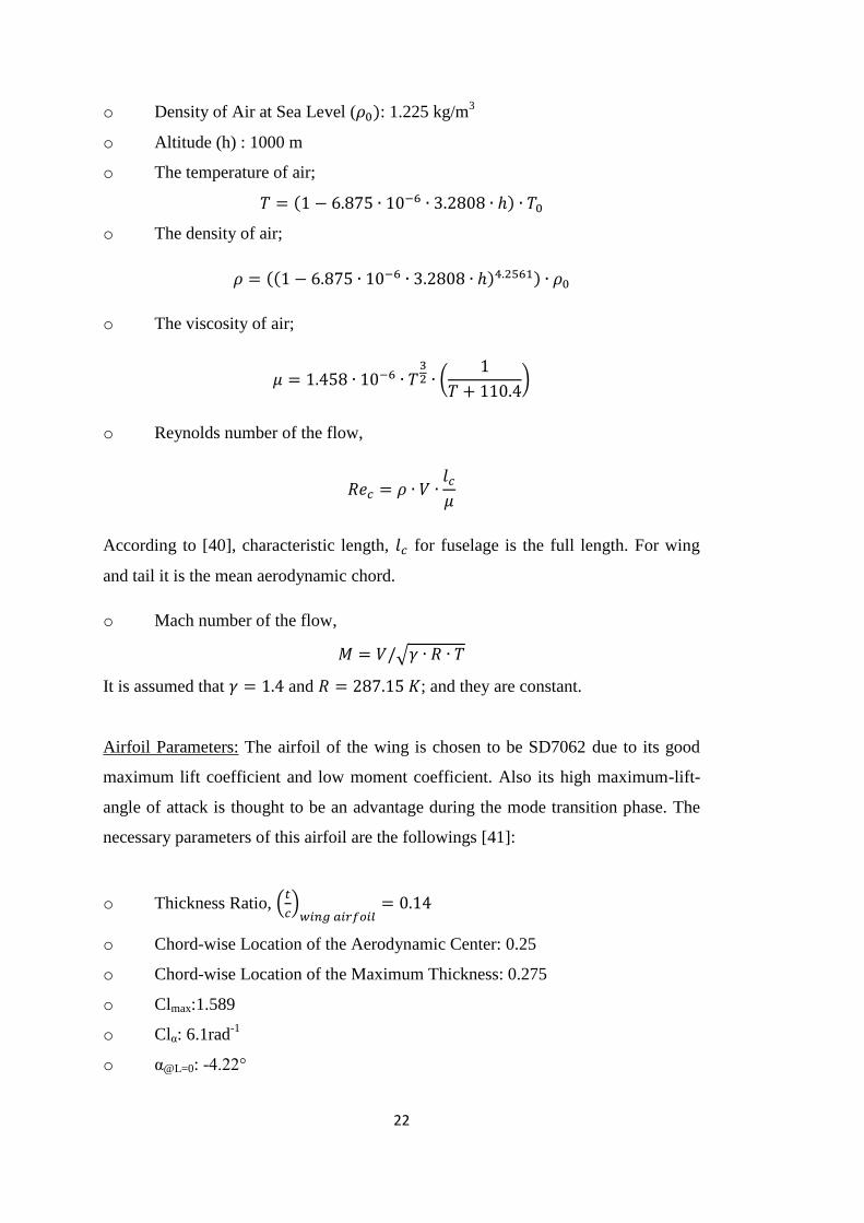
22

o Density of Air at Sea Level ( : 1.225 kg/m3

o Altitude (h) : 1000 m

o The temperature of air;

(

o The density of air;

((

o The viscosity of air;

(

)

o Reynolds number of the flow,

According to [40], characteristic length, for fuselage is the full length. For wing

and tail it is the mean aerodynamic chord.

o Mach number of the flow,

√

It is assumed that and ; and they are constant.

Airfoil Parameters: The airfoil of the wing is chosen to be SD7062 due to its good

maximum lift coefficient and low moment coefficient. Also its high maximum-lift-

angle of attack is thought to be an advantage during the mode transition phase. The

necessary parameters of this airfoil are the followings [41]:

o Thickness Ratio, (

)

o Chord-wise Location of the Aerodynamic Center: 0.25

o Chord-wise Location of the Maximum Thickness: 0.275

o Clmax:1.589

o Clα: 6.1rad-1

o α@L=0: -4.22°

23

Table 2.1 Airfoil Comparison @ Re=200000 [41]

WB-

135/35

USA 28

SD7062

S3021-095-84

S1223

HQ 3.5/14

GOE 655 GOE 575

FX 63-137

E214

Thickness (%)

13.529 13.16 13.968 9.467 12.067 13.999 13.88 13.348 13.635 11.093

Camber (%)

3.767 3.754 3.981 2.959 8.692 3.527 4.399 3.608 5.988 4.043

Trailing Edge Angle

(%) 14.869 20.991 6.301 7.285 7.683 12.018 15.446 35.021 5.675 9.066

Lower Surface Flatness

71.94 81.625 81.518 91.326 17.624 71.535 89.352 85.186 66.522 86.62

Leading Edge

Radius (%) 3.458 3.419 2.727 1.779 3.104 2.545 3.999 4.056 2.152 1.891

Maximum Lift (CL)

1.41 1.345 1.589 1.122 2.425 1.595 1.646 1.744 2.037 1.549

Maximum Lift Angle-of-Attack

(deg)

11 15 15 8 8 11.5 15 10.5 11.5 9

Maximum Lift-to-

drag (L/D) 51.679 62.786 52.55 57.274 125.35 63.14 58.202 60.648 97.886 87.641

Lift at Maximum

Lift-to-drag

1.2 0.882 0.974 0.821 2.131 1.351 1.098 0.985 1.319 0.973

Angle-of-Attack for Maximum

Lift-to-drag (L/D)

7.5 3.5 4.5 4.5 5 6.5 4.5 4 2 2.5

Figure 2.5Polars of SD7062 @Re=200000[41]

http://www.airfoildb.com/foils/6















24

The airfoil chosen for the horizontal and vertical tail is NACA 0009, and the

necessary parameters of this airfoil are the followings:

o Thickness Ratio, (

)

(

)

o Chord-wise Location of the Aerodynamic Center: 0.25

o Chord-wise Location of the Maximum Thickness: 0.3

o Clα: 5.58 rad-1

Power Calculation Inputs: A high energy density lithium-polymer battery is chosen

for feeding the propulsion unit. The inputs related to it are the followings [37]:

o Nominal Voltage,

o Capacity,

o Battery Count,

o Vertical Flight Power Consumption: According to the datasheet of the chosen

brushless D/C motor (see APPENDIX B), an average value can be approximated for

endurance calculations.

o Motor Maximum Continuous Power, [42]

Aerodynamic Inputs:

o Wing Aspect Ratio: The aspect ratio of the wing is a key design parameter,

and it is given various values to create different design cases. By the outcome of the

literature survey, wing aspect ratio will be in a range between 6 and 13.

{ }

o Wing Loading: Another key parameter is the wing loading of the aircraft. It is

also given different values to set various design cases. By the outcome of the

literature study, the wing loading will be given values in a range between 80 and 200

N/m2

{ }

o Velocity: The design velocity parameter is considered as the trim velocity at

cruise with no angle of attack. Besides, it is possible to set a range for the velocity

parameter for different optimization goals. In optimization phase, velocity is 20 m/s

25

and constant; but the domain to be analyzed is created to include the variation of the

velocity within the range of 20 m/s and 30m/s.

{ }

o Horizontal and Vertical Tail Aspect Ratios: Although they might need to be

revised after analyzing the prop-wash effects of the propellers by wind tunnel test or

numerical methods; for the early phases of the design the aspect ratio of the

horizontal and vertical tail is determined from [40] and fixed to those typical values.

o Wing Taper Ratio: According to the [40], for most unswept wings a taper

ratio of around 0.4 is ideal considering the lift distribution tailoring and weight

reduction effects of the taper. In this specific case, in order to increase the clearance

between the propellers and the wing; a higher but still a typical value of wing taper

ratio is set.

o Horizontal and Vertical Tail Taper Ratios: The taper ratios of the horizontal

and vertical tails are determined according to the typical values mentioned in [40].

o Volume Ratios of the Horizontal and Vertical Tail: For the initial phases the

volume ratios are determined from [40]. On the other hand, according to the stability

and maneuverability requirements of a possible controller design, there might be a

need of revision.

o Wing Dihedral, Twist and Sweep Angles: Considering the manufacturing

easiness and the flight regime of the aircraft, the dihedral and the twist angles of the

wing are taken to be zero. In addition to that, for an easier structural integrity, the

sweep angle at the quarter chord of the wing, where the main spar is located, is zero.

Motor and Tail Booms Parameters: These parameters are directly imposed and

determined at the beginning of the design phase.

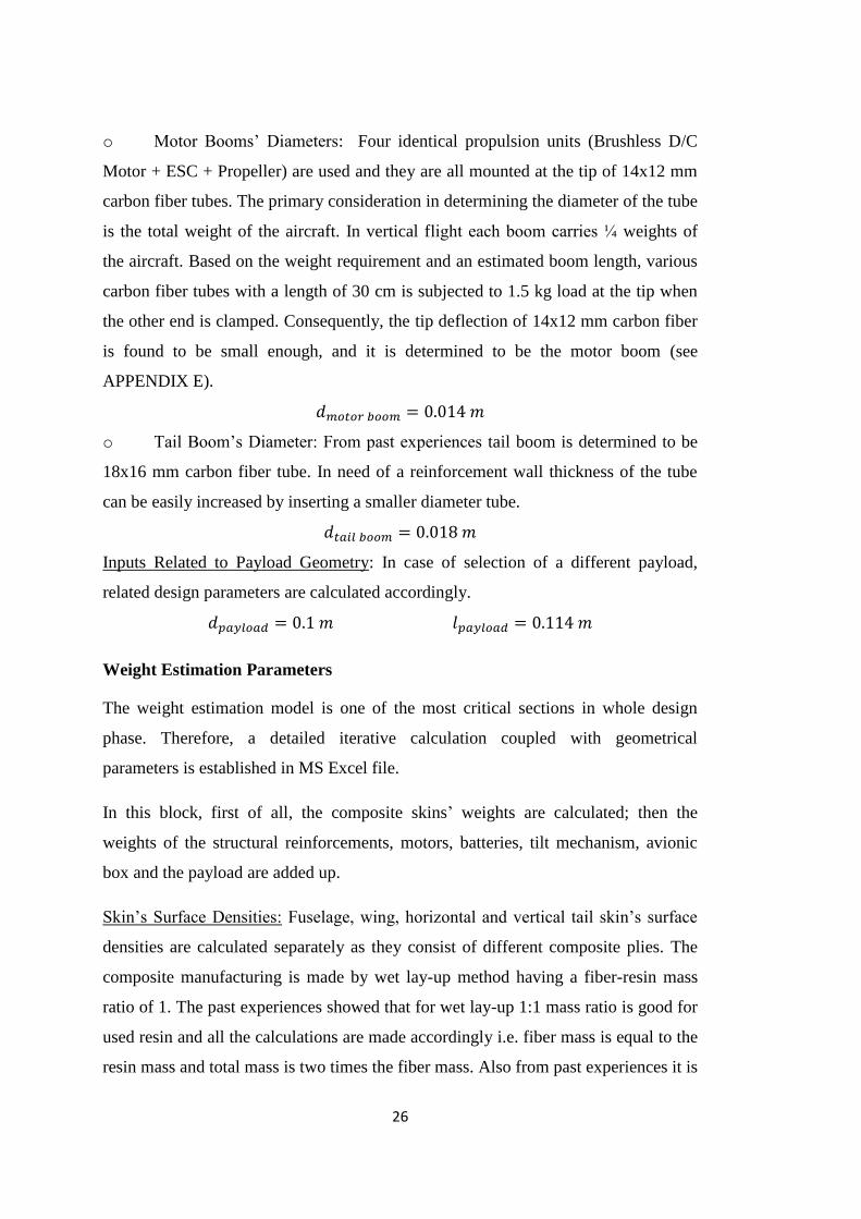
26

o Motor Booms’ Diameters: Four identical propulsion units (Brushless D/C

Motor + ESC + Propeller) are used and they are all mounted at the tip of 14x12 mm

carbon fiber tubes. The primary consideration in determining the diameter of the tube

is the total weight of the aircraft. In vertical flight each boom carries ¼ weights of

the aircraft. Based on the weight requirement and an estimated boom length, various

carbon fiber tubes with a length of 30 cm is subjected to 1.5 kg load at the tip when

the other end is clamped. Consequently, the tip deflection of 14x12 mm carbon fiber

is found to be small enough, and it is determined to be the motor boom (see

APPENDIX E).

o Tail Boom’s Diameter: From past experiences tail boom is determined to be

18x16 mm carbon fiber tube. In need of a reinforcement wall thickness of the tube

can be easily increased by inserting a smaller diameter tube.

Inputs Related to Payload Geometry: In case of selection of a different payload,

related design parameters are calculated accordingly.

Weight Estimation Parameters

The weight estimation model is one of the most critical sections in whole design

phase. Therefore, a detailed iterative calculation coupled with geometrical

parameters is established in MS Excel file.

In this block, first of all, the composite skins’ weights are calculated; then the

weights of the structural reinforcements, motors, batteries, tilt mechanism, avionic

box and the payload are added up.

Skin’s Surface Densities: Fuselage, wing, horizontal and vertical tail skin’s surface

densities are calculated separately as they consist of different composite plies. The

composite manufacturing is made by wet lay-up method having a fiber-resin mass

ratio of 1. The past experiences showed that for wet lay-up 1:1 mass ratio is good for

used resin and all the calculations are made accordingly i.e. fiber mass is equal to the

resin mass and total mass is two times the fiber mass. Also from past experiences it is

27

known that in wet lay-up method, it is very hard to prevent the core material to

absorb the resin; and it is a good practice to take the weight of resin used to adhere

the core material is equal to the weight of the core material itself. In other words,

also the mass fraction of the core material and resin is 1. In addition to that, skins are

not isotropic and at some structurally critical zones, reinforcements are applied.

Hence, skin surface densities are calculated according to the formula:

∑(

(

(

o Fuselage Skin Surface Density: The fuselage skin has the plies shown by

Figure 2.6. It is determined to reinforce the critical structural junction points with the

wing, tail boom and the motor booms. Apart from the inner structure, at these

locations, skin has a different laminate shown by the same figure. From the initial

CAD drawings it is estimated that 50% of the fuselage surface has reinforcement.

Thus, the average surface density is calculated accordingly.

Figure 2.6Fuselage Skin Plies (without -on the left hand side- and with reinforcement -on the right hand side-)

(( )

(( )

25 gr/m2 E-glass Fiber

61 gr/m2

Aramid Fiber

49 gr/m2

E-glass Fiber

44 gr/m2

Aramid Honeycomb (1mm)

49 gr/m2

E-glass Fiber

61 gr/m2

Aramid Fiber

49 gr/m2

E-glass Fiber

93 gr/m2

Carbon Fiber

44 gr/m2

Aramid Honeycomb (1.5 mm)

25 gr/m

2

E-glass Fiber

44 gr/m2

Aramid Honeycomb (1.5 mm)

49 gr/m

2

E-glass Fiber

25 gr/m2

E-glass Fiber

28

o Wing Skin Surface Density: The wing skin is composed of the plies shown by

the Figure 2.7. It is determined to reinforce the wing root by adding a carbon fiber

ply with area of 20% of the total wing surface.

Figure 2.7Wing Skin Plies (without -on the left hand side- and with reinforcement -on the right hand side-)

(( ) (( )

o Horizontal Tail Skin Surface Density: The horizontal tail skin is composed of

the plies shown by the Figure 2.8. It is determined to reinforce the boom connection

section of the horizontal tail by adding two carbon fiber plies with area of 25% of the

total horizontal tail surface. At that zone, there is no core material.

Figure 2.8Horizontal and Vertical Tail Skins Plies (without -on the left hand side- and with reinforcement -on the

right hand side-)

(( ) (( )

o Vertical Tail Skin Surface Density: The vertical tail skin is composed of the

plies shown by the Figure 2.8. It is determined to reinforce the boom connection


49 gr/m2

E-glass Fiber

31 gr/m

2

Rohacell Foam (1 mm)

49 gr/m2

E-glass Fiber

25 gr/m2

E-glass Fiber

49 gr/m2

E-glass Fiber

93 gr/m

2

Carbon Fiber

93 gr/m

2

Carbon Fiber

49 gr/m2

E-glass Fiber


49 gr/m2

E-glass Fiber

31 gr/m

2


49 gr/m2

E-glass Fiber

25 gr/m2

E-glass Fiber

49 gr/m2

E-glass Fiber

31 gr/m

2


93 gr/m2

Carbon Fiber

49 gr/m2

E-glass Fiber

29

section of the vertical tail by adding two carbon fiber plies with area of 40% of the

total vertical tail surface. At that zone, there is no core material.

(( ) (( )

Skin’s Wetted Areas: Geometric outputs of the iterative calculations feed this block

and from reference area values wetted areas are calculated.

o Fuselage Wetted Area: Fuselage is approximated as a cylinder.

( )

o Wing and Tail Wetted Area: According to [44], note that the second

multiplier in the formula is the exposed wing area.

( (

)

(

( (

)

( (

)

Composite Part Weights: The composite part weights indicate the weight of the

assembled parts with structural reinforcement. In other words, it is the total weight

including outer skin and inner structure (ribs, spars, bulkheads etc.) As an important

note, the painting is not included in calculations. The reason for this situation is that

in a real production case the painting is planned to be done by adding colour

pigments into the resin, which is assumed to have very small contribution to the total

weight. The painting is not so critical for such an aircraft, and it is unnecessary to

make the aircraft heavier with additional putty and painting operations. Otherwise, as

deduced from past experiences, painting is a very uncontrollable process for such a

small aircraft, and it is not preferable.

o Fuselage Weight: Two separately produced fuselage sides are assembled with

polyurethane adhesive. Also, inside the fuselage there are carbon fiber tubes at the

30

junction points of the wing, tail and motor booms; and these tubes are supported with

balsa/e-glass plates.

According to the initial CAD drawings, the total area of the reinforcement plates to

be used inside the fuselage is very close to the largest cross section of the fuselage.

By formulating the relation in this way, the linkage between fuselage dimensions and

the area of the inner structure is kept.

There are booms located centrically to mount the wing spars and the tail boom. The

tail boom is assumed to be inserted 10 cm into the fuselage boom in any case.

The adhesive weight is calculated from the lengths of the lines, where adhesive is

applied. From the initial CAD drawings, it is found appropriate to approximate the

inner structure of the fuselage as “circular bulkheads placed along the fuselage with

10 cm between them”. By this way, the total length of the inner structure parts’ sides

is approximated depending on related parameters of fuselage length and diameter.

(( ) )

(

)

( (

))

o Wing Weight: Assembled wing part is composed of composite upper and

lower skins, ribs made from the same reinforcement plate used inside the fuselage,

carbon fiber tubes with different sizes and the adhesive material.

From past experiences, it is assumed that an average distance of 8 cm between ribs is

a good enough for such an aircraft. In addition to that, from the initial CAD drawings

it is seen that the total area of the ribs is in order of 10% of the reference area of the

wing. This proportion depends on the wing span, thickness ratio of the airfoil and

wing taper ratio. Within a small enough range, this proportion is assumed to be more

or less applicable.

As the wing is tapered, its thickness is decreasing through the tip; so the diameters of

the carbon fiber tubes are decreasing gradually. From the initial CAD drawings,

average lengths of the tubes are determined with respect to the wing span. In design

aspect, this correlation between wing span and carbon fiber tubes contributes to

31

proportionality between the aspect ratio and the weight of the wing, which is a

demand of the structural side [40].

The length to be applied adhesive is the periphery of the wing added up to the ribs’

upper and lower sides. Note that, as assumed before, the ribs are thought to be

located with average 8 cm between them.

(

)

(

(

(

(

(

( ( (

( (

{ ( ) [( )

]

}

o Horizontal and Vertical Tail Weights: Assembled horizontal and vertical tails

are composed of upper and lower (or right and left) skins, inner structure made of the

reinforcement plate and adhesive material.

The length to be applied adhesive is calculated in a same manner with the wing, and

in addition to that tail boom interfaces are added to the formulas. The tail boom goes

all below the vertical tail and into the half of the horizontal tail. Note that upper and

lower sides of the boom are adhered to the surfaces.

The spar lengths are approximated to be equal to the tail spans; and note that upper

and lower sides of the spar are adhered to the surfaces.

(

)

[ (

( (

]

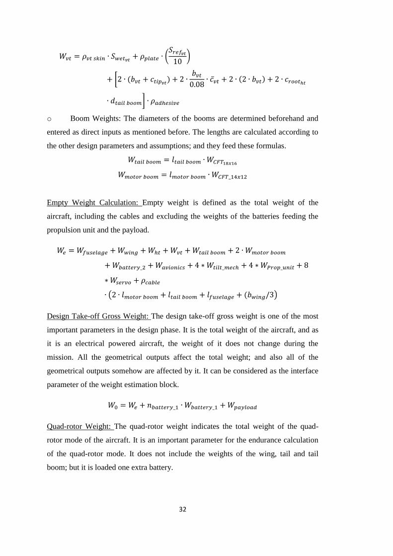
32

(

)

[ (

(

]

o Boom Weights: The diameters of the booms are determined beforehand and

entered as direct inputs as mentioned before. The lengths are calculated according to

the other design parameters and assumptions; and they feed these formulas.

Empty Weight Calculation: Empty weight is defined as the total weight of the

aircraft, including the cables and excluding the weights of the batteries feeding the

propulsion unit and the payload.

( ( )

Design Take-off Gross Weight: The design take-off gross weight is one of the most

important parameters in the design phase. It is the total weight of the aircraft, and as

it is an electrical powered aircraft, the weight of it does not change during the

mission. All the geometrical outputs affect the total weight; and also all of the

geometrical outputs somehow are affected by it. It can be considered as the interface

parameter of the weight estimation block.

Quad-rotor Weight: The quad-rotor weight indicates the total weight of the quad-

rotor mode of the aircraft. It is an important parameter for the endurance calculation

of the quad-rotor mode. It does not include the weights of the wing, tail and tail

boom; but it is loaded one extra battery.

33

( ) (

Drag Estimation Parameters

Based on geometrical parameters, drag estimation parameters contribute the

performance calculations. According to the drag build-up method, each component’s

parasite drag is found separately, and then the total value is sent to the performance

block to calculate the drag coefficient from the drag polar. All the formulas below

are taken or derived from [40].

∑( )

Skin friction coefficient for turbulent flows is formulated as,

( (

Form factor for wing and tail is formulated as,

[

( )

(

) (

)

] [ ( ]

For wing and tail surfaces, the sweep angles at maximum thicknesses are calculated

considering the fact that the sweep at the quarter chord and the sweep at the trailing

edge is zero, respectively. For the tail surfaces, the sweep angle at the trailing edge is

zero in order to ease the manufacturing of the control surfaces.

Form factor of the fuselage is formulated as,

[

]

According to [45] the drag coefficient of a cylinder can be taken as roughly 0.5

between Re=104-10

6. If it is normalized according to the reference areas of the motor

booms and the wing,

34

[ ( ]

Geometrical Output Parameters

All of the geometrical outputs are calculated iteratively. When they are found, they

feed back the weight and drag estimation parameters. All the lengths and areas are

calculated in this block. Generic formulas are taken from [40].

Basic Lengths:

o Fuselage Length: The main design constraint of the fuselage is the clearance

between wing and propellers. So, the wing root chord and the possible propeller

diameter are design inputs here. The length of one propeller diameter has to be

covered by the fuselage at minimum; so 1.5 half of the propeller diameter is taken as

input. In fuselage design that choice is going to be considered. The propeller

diameter is chosen to be 12’’ (~0.3 m) initially, and as a conservative approach the

root chord is used as reference length.

o Fuselage Diameter: The reference value for fuselage diameter depends on the

payload (here a gimbal) diameter. There should be enough space to mount the

gimbal, which is equal to the payload diameter minimum; and 2 cm of extra length is

assumed for lofting of the aerodynamic surface.

o Length of the Motor Booms: As the booms go all along the fuselage, the

fuselage diameter is an input and considering the clearance between propellers and

fuselage, ¼ length of the propeller diameter is left at each side.

o Length of the Tail Boom: The horizontal and vertical tails are located in

sequence on the tail boom (boom ends at the middle of the horizontal tail); so the

root chords of them are inputs. Besides, a 15 cm of clearance between fuselage and

vertical tail is assumed initially.

35

o Spans: Wing and tail spans are calculated as follows, (subscript “c” refers to

“component”)

√

o Chords: Wing and tail chords are calculated as follows,

Surface Areas:

o Wing Reference Area: It is one of the most important and influential output

parameter.

(

o Horizontal Tail Reference Area: The wing quarter chord is assumed to be at

the middle of the fuselage; and the tail arm is calculated accordingly.

(

o Vertical Tail Reference Area: A same logic as the horizontal tail is used here.

(

(

Angle of Incidence: According to the necessary cL value, a set angle is calculated to

give an idea for orienting the wing with respect to the fuselage. The first model is

going to be drawn and the prototype is going to be produced according to this set

angle.

36

Performance Output Parameters

The outputs of this block do not affect other calculations; so they can be considered

as the results. Generic formulas, which are for fixed a wing aircraft, are taken from

[40]. Prop-wash effects of the rotors are not included in these calculations.

Force Coefficients:

o Lift Coefficient: It is directly calculated from the basic inputs without

iteration.

(

o Drag Coefficient: It is calculated from the drag polar as follows,

Here,

o The Oswald efficiency factor for a wing with is formulated as,

( )

o Maximum Lift Coefficient: It is calculated as follows,

(

Lift Curve Slope: The total lift curve slope From [43]:

( (

)

)

o Lift curve slope of the wing-body combination:

( (

)

(

))

o Lift curve slope of the wing and horizontal tail:

√(

(

)

37

√

(

)

o The downwash factor is calculated as,

(

| )

|

|

|

|

[ √ ]

( )

( ( (

)

)

From the initial sketches it is assumed that

Thrust and Power Required: For required power calculation typical efficiency factors

for propellers and D/C motors are assumed. [46] The ideal power consumption can

be thought as the power output; the power required is the input power for the motors

and must be drawn from the system. Therefore, the power required is used in all

calculations rather than the ideal value.

38

Power Available: According to [47], about 70% of the maximum thrust should be

enough for vertical flight. It means that the 70% of the total maximum static thrust

values of the motors must be equal to the total weight of the aircraft. The motor

selection is made according to this requirement [47], [11]. So, thrust to weight ratio

is happened to be an initial design choice independently from the rate of climb or

maximum speed, which are not critical in this aircraft concept. The total power

available is the sum of four motors powers’ multiplied by motor and propeller

efficiencies.

From the motor propeller data (see Appendix B), it can be deduced that the assumed

efficiency values, which are in fact the typical ones, are in a good match with the real

cases.

Endurances: In hovering, it is assumed that the aircraft consumes a constant amount

of power,

, determined by vertical flight power consumption value. This

constant amount is a function of the total weight, and it is assumed to be linearly

increasing with the total weight. The horizontal flight endurances are calculated by

dividing the total energy capacity (after subtracting the energy spent during the

hovering time) by power required.

o Mission 1 (Horizontal Flight): It is assumed that total time spent for take-off

and landing is 30 seconds. (

[

]

o Mission 2 (Vertical Flight in Fixed Wing Mode):

[

]

o Mission 3 (Vertical Flight in Quad-rotor Mode):

[

(

]

o Mission 4 (Special Mission Flight): It is assumed that total time spent for

take-off and landing is 30 seconds. (

39

[

]

Stall Speed: It is an important parameter in optimization phase in terms of controlling

the wing loading; and it is calculated as follows,

√

Rate of Climb: As the propulsion unit is chosen for vertical flight capability, the rate

of climb values are expected to be higher for a mini class UAV. It is calculated as

follows,

⁄

Maximum Velocity: Maximum velocity is calculated by finding the point where drag

is equal to the available thrust, which is a function of velocity. So, there needs to be

an iterative calculation to find the corresponding lift coefficient and available thrust

value.

√

(

)

Maximum Load Factor: The load factor is a function of velocity and it is constraint

by available power and maximum lift coefficient. The value of the load factor is

calculated according to the limitations of both factors, and the smaller value is

accepted as the maximum load factor at that velocity.

( ⁄ or

[

( ⁄ (

( ⁄ )]

⁄

40

At low velocities, the maximum load factor is limited by the maximum lift

coefficient; and at high velocities the available power limits it. The velocity where

the limiting factor shifts is called the corner velocity, and it is very important for

maneuvering calculations. It can be thought as the best maneuvering velocity.

√

(

)

Maximum Turn Rate and Minimum Turn Radius:

√

(

√

2.3 Determination of Inputs, Outputs and Optimization Criteria

In consideration of the requirements, design criteria are determined; inputs and

outputs are defined accordingly. As it is explained in the first chapter, the main

purpose of the aircraft is surveillance, and the primary performance goal is

endurance, rather than the maximum speed or manoeuvring capabilities. Both

horizontal and vertical flight times are considered in the optimization phase by

defining constraints and objectives on the necessary parameters.

Figure 2.9Defined Parameters in Excel Interface of Ansys Workbench

41

Wing Loading: The most coupling parameter of the model is the wing loading. It

determines the wing reference area, which is the main geometrical output, directly

from the total weight. Wing loading is selected to be an input in Ansys Workbench

side. The parameter name is assigned as “WING_LOADING”. A wide range

(between 80 and 200 N/m2 ) is determined by the competitor study.

Wing Aspect Ratio: The second important parameter is the aspect ratio of the wing, it

affects the wing span and thereby the span efficiency of the wing. So the drag and the

endurance calculations are affected. In addition to that the total weight is also slightly

affected by the aspect ratio. It is also defined as an input as it can be seen in Figure

2.9, and its name is “WING_ASPECT_RATIO”. The range to be analysed of it is

between 6 and 13.

Velocity: In fact, the design cruise velocity of the aircraft does not affect the

geometry or weight parameters in the mathematical model. Only the possible wing

incidence angle is calculated using the velocity. On the other hand, the dominant

factor in endurance calculations is the velocity by far. If there is no objective on the

design cruise velocity, the optimization phase gives always candidates with the

lowest ones. In light of the competitor study, 20 m/s of cruise velocity is determined

to be an appropriate value. Considering that the operational range is about 15 km,

trading the endurance for velocity is not very sensible. However, it is a good practice

to see the effects of the velocity changes on the output parameters, so the design

cruise velocity is also defined as input and the response curves are created for

velocity variations between 20 m/s and 30 m/s. In optimization phase the velocity is

kept constant as 20 m/s. The name of this parameter in Ansys Workbench side is

“VELOCITY”.

Stall Speed: For this concept, landing and take-off distance are not applicable and the

maximum speed is not a primary requirement. So, the most important performance

parameter to constrain the wing loading is the stall speed. It is also important to

minimize the stall speed considering the mode transition from vertical flight to

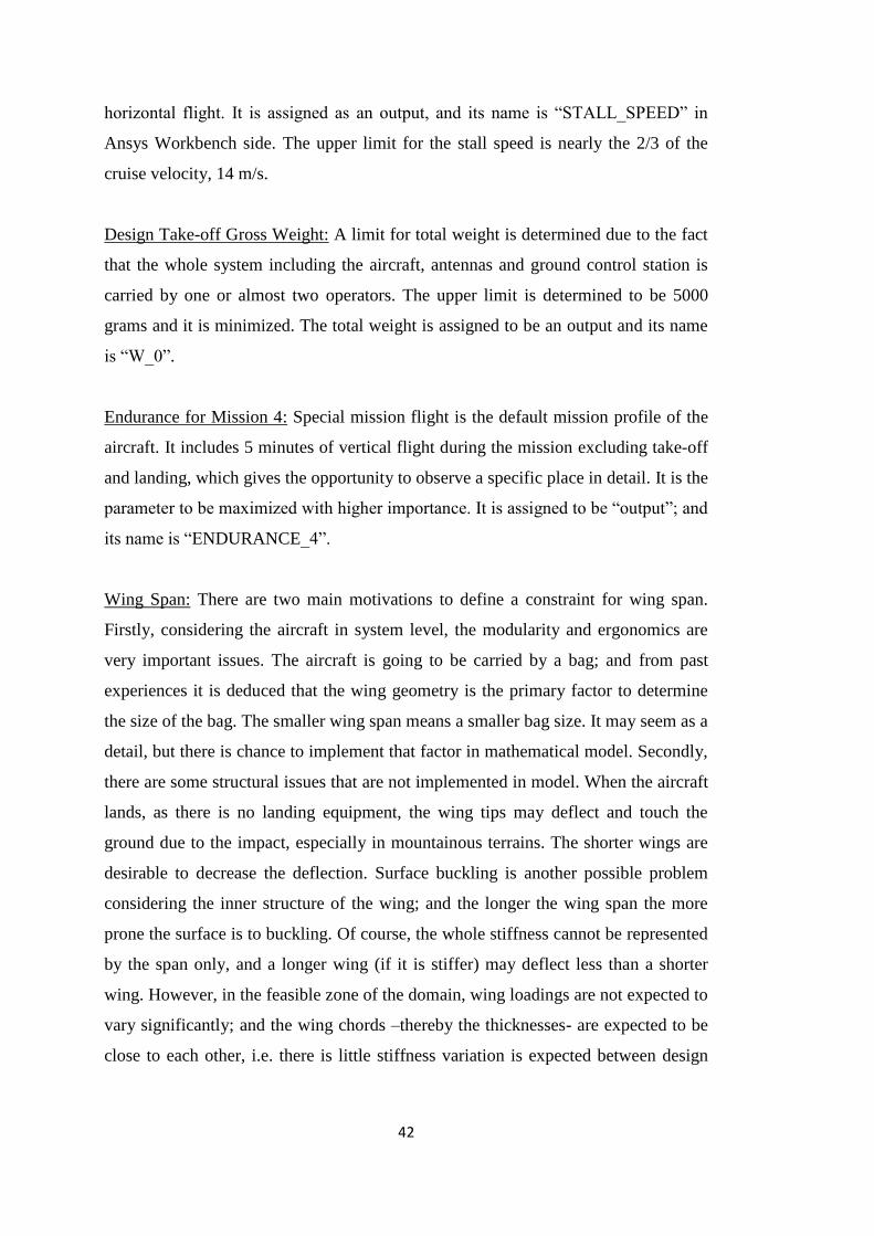
42

horizontal flight. It is assigned as an output, and its name is “STALL_SPEED” in

Ansys Workbench side. The upper limit for the stall speed is nearly the 2/3 of the

cruise velocity, 14 m/s.

Design Take-off Gross Weight: A limit for total weight is determined due to the fact

that the whole system including the aircraft, antennas and ground control station is

carried by one or almost two operators. The upper limit is determined to be 5000

grams and it is minimized. The total weight is assigned to be an output and its name

is “W_0”.

Endurance for Mission 4: Special mission flight is the default mission profile of the

aircraft. It includes 5 minutes of vertical flight during the mission excluding take-off

and landing, which gives the opportunity to observe a specific place in detail. It is the

parameter to be maximized with higher importance. It is assigned to be “output”; and

its name is “ENDURANCE_4”.

Wing Span: There are two main motivations to define a constraint for wing span.

Firstly, considering the aircraft in system level, the modularity and ergonomics are

very important issues. The aircraft is going to be carried by a bag; and from past

experiences it is deduced that the wing geometry is the primary factor to determine

the size of the bag. The smaller wing span means a smaller bag size. It may seem as a

detail, but there is chance to implement that factor in mathematical model. Secondly,

there are some structural issues that are not implemented in model. When the aircraft

lands, as there is no landing equipment, the wing tips may deflect and touch the

ground due to the impact, especially in mountainous terrains. The shorter wings are

desirable to decrease the deflection. Surface buckling is another possible problem

considering the inner structure of the wing; and the longer the wing span the more

prone the surface is to buckling. Of course, the whole stiffness cannot be represented

by the span only, and a longer wing (if it is stiffer) may deflect less than a shorter

wing. However, in the feasible zone of the domain, wing loadings are not expected to

vary significantly; and the wing chords –thereby the thicknesses- are expected to be

close to each other, i.e. there is little stiffness variation is expected between design

43

points. Considering all, the wing span is minimized with lower importance. The

wing span is an output and its name is “WING_SPAN” in Ansys Workbench side.

Endurance for Mission 1: The endurance of the horizontal flight in fixed wing mode

is not subjected to a design objective, but the lower values of this parameter are not

accepted. Therefore a lower boundary of 90 minutes is assigned to it. It is also an

output, and its name is “ENDURANCE_1”.

Endurance for Mission 3: The vertical flight endurance in quad-rotor mode is also

maximized. It is directly a result of the quad-rotor weight. In addition to it, there is a

loose correlation between the wing aspect ratio as the length of the fuselage is

dependent on the wing root chord. It is an output to be maximized in the optimization

phase and its name is “ENDURANCE_3”.

Endurance for Mission 2: The endurance of the vertical flight in fixed wing mode is

an exceptional case that might happen in marginal operations. Also, it is a direct

function of the total weight of the aircraft only. So it is meaningless to assign a

maximizing objective to it. However, it is important to know the endurance limit for

vertical flight; as it might be necessary to lengthen the vertical flight at the instant of

operation. It is defined as an output to create the response curves, but it does not have

any effect in the optimization phase. Its name is “ENDURANCE_2” in Ansys

Workbench side.

Quad-rotor Weight: Like the endurance of the vertical flight in fixed wing mode, the

effect of the quad-rotor weight is already included by “ENDURANCE_3” parameter.

So, it is also defined as an output and its response curves are created; but it has no

effect in the optimization phase. Its name is “W_quad”.

Battery Count: In initial optimization studies, the battery count was an input

parameter that can have only discrete values. The values of 2, 3 and 4 batteries are

tried. As outcome, it was very clear that the candidates with 2 or 4 batteries are

always eliminated by the design requirements. The options with four batteries make

the aircraft exceed the weight requirement; and the options with two batteries do not

44

satisfy the endurance requirements. To sum up, battery count is not defined in Ansys

Workbench side; its value is 3 and it is constant.

Table 2.2 Defined Parameters in Optimization Toolbox and Optimization Criteria

PARAMETER

OBJECTIVE

OBJECTIVE

IMPORTANCE

LOWER

BOUND

CONSTRAINT

UPPER BOUND

CONSTRAINT

WING_LOADING - - - -

WING_ASPECT_RATIO - - - -

VELOCITY - - - -

STALL_SPEED Minimize Default - 14 m/s

W_0 Minimize Default - 5000 gr

ENDURANCE_4 Maximize Higher - -

WING_SPAN Minimize Lower - 2 m

ENDURANCE_1 - - 90 min -

ENDURANCE_3 Maximize Default - -

ENDURANCE_2 - - - -

W_quad - - - -

As it can be seen in Table 2.2, “ENDURANCE_4” has the higher importance. So

maximizing objective for it can be seen as the main objective; and the other ones are

complementary objective. The objective importances are determined after a long

term of optimization runs with different settings. The mechanism of this option is

well described in [48].

In a nutshell, the primary objective is to maximize the combined flight endurance;

while maximizing the quad-rotor mode’s endurance and minimizing the total weight,

stall speed and wing span with lower priorities. No numerical values can be

implemented regarding to their “objective importances”, but pre-defined priority

options, which are “lower”, “higher” and “default”, can be selected to tune the

optimization process. These selections are made according to many trials and [48].

45

2.4 Procedure in Ansys Workbench Design Exploration Toolbox

In Ansys Workbench, inside the Design Exploration toolbox, “Response Surface

Optimization” procedure is conducted. This procedure includes three phases. At first,

the data is extracted from Excel file in a predetermined method, and then this data is

interpolated and used to create a response surface for the model. Lastly, by defining

the desired optimization criteria, toolbox chooses the best candidates for the project.

Design of Experiments

The first step in Response Surface Optimization is the design of experiments. At the

beginning of the optimization study, a case domain (domain of different design

cases) must be defined. In this defined case domain, all the correlations between

parameters are going to be identified and the trends are going to be revealed by the

program, i.e. the program learns the relations between parameters. Only after that the

optimization phase can decide the best case for the given requirements.

First of all, the limits of the domain are defined by entering ranges for the input

parameters. Then according to the selected method, sampling points to be analysed

are determined. At that point, Ansys Workbench calls MS Excel and uses it as solver

to make all the calculations. The calculations are made according to the formulas

embedded in MS Excel file.

Figure 2.10The Procedure in Design of Experiments Phase

The ranges for the inputs are stated in the previous section. Here it is determined that

the domain is continuous, which means that the input parameters do not have to be

integers, but they may have any value.

The method for sampling depends on the type of the design of experiments. The most

appropriate option is determined from [48] and numerous trials. “Central Composite

Define the upper and lower limits of the input parameters.

(Velocity, Wing Loading and wing

Aspect Ratio)

Determine the sampling method and create the sampling

points

Call MS Excel to solve for the output

parameters at the sampling points

46

Design” type is selected. “Rotatable” algorithm with “Enhanced” template is

selected.

The output of the design of experiments phase is shown below. Note that, the design

of experiments table can be filled manually by running MS Excel separately and

noting down the output values one by one.

Table 2.3 Output of Design of Experiments

CASE

V (m/s) AR

W/S (N/m

2)

E_1 (min)

E_2 (min)

E_3 (min)

E_4 (min)

V_STALL (m/s)

W_0 (gr)

W_quad (gr) b (m)

1 25 9.5 140.0 65.0 16.5 27.91 44.70 13.19 4959.8 3909.5 1.82

2 20 9.5 140.0 101.7 16.5 27.91 69.92 13.19 4959.8 3909.5 1.82

3 22.5 9.5 140.0 81.7 16.5 27.91 56.15 13.19 4959.8 3909.5 1.82

4 30 9.5 140.0 41.6 16.5 27.91 28.61 13.19 4959.8 3909.5 1.82

5 27.5 9.5 140.0 51.8 16.5 27.91 35.64 13.19 4959.8 3909.5 1.82

6 25 6 140.0 61.9 16.6 27.74 42.66 13.19 4929.9 3933.7 1.44

7 25 7.75 140.0 63.9 16.553 27.84 43.97 13.19 4943.9 3919.5 1.64

8 25 13 140.0 66.1 16.39 28.01 45.28 13.19 4993 3896.0 2.13

9 25 11.2 140.0 65.7 16.445 27.97 45.09 13.19 4976.3 3901.9 1.98

10 25 9.5 80.0 61.4 14.844 27.65 40.00 9.97 5513 3947.0 2.53

11 25 9.5 110.0 64.2 15.885 27.81 43.36 11.69 5151.7 3923.7 2.09

12 25 9.5 200.0 64.1 17.203 28.03 44.91 15.76 4757.2 3892.3 1.49

13 25 9.5 170.0 64.8 16.909 27.98 45.07 14.53 4839.8 3899.6 1.63

14 22.02 7.41 104.3 83.3 15.806 27.68 56.11 11.38 5177.6 3941.8 1.90

15 23.51 8.45 122.2 73.7 16.203 27.81 50.25 12.32 5050.6 3923.3 1.85

16 27.97 7.41 104.3 47.9 15.806 27.68 32.28 11.38 5177.6 3941.8 1.90

17 26.48 8.45 122.2 56.0 16.203 27.81 38.19 12.32 5050.6 3923.3 1.85

18 22.02 11.5 104.3 86.7 15.654 27.86 58.06 11.38 5227.8 3916.8 2.39

19 23.51 10.5 122.2 75.0 16.134 27.89 51.03 12.32 5072.5 3912.1 2.07

20 27.97 11.5 104.3 48.3 15.654 27.86 32.34 11.38 5227.8 3916.8 2.39

21 26.48 10.5 122.2 56.5 16.134 27.89 38.45 12.32 5072.5 3912.1 2.07

22 22.02 7.41 175.7 79.4 17.027 27.92 55.39 14.77 4806.3 3909.0 1.41

23 23.51 8.45 157.8 73.1 16.791 27.92 50.64 14.00 4873.9 3908.5 1.60

24 27.97 7.41 175.7 49.1 17.027 27.92 34.27 14.77 4806.3 3909.0 1.41

25 26.48 8.45 157.8 56.5 16.791 27.92 39.13 14.00 4873.9 3908.5 1.60

26 22.02 11.5 175.7 85.6 16.915 28.05 59.53 14.77 4838.3 3890.3 1.77

27 23.51 10.5 157.8 74.9 16.731 27.99 51.85 14.00 4891.5 3898.8 1.79

28 27.97 11.5 175.7 50.6 16.915 28.05 35.16 14.77 4838.3 3890.3 1.77

29 26.48 10.5 157.8 57.3 16.731 27.99 39.65 14.00 4891.5 3898.8 1.79

47

Response Surface

The second step is creating a response surface. The output of the design of

experiments is taken in Response Surface section. The trends are determined from

the design of experiments data and necessary interpolations and extrapolations are

performed. So, the whole domain is covered. For rather complicated studies or in

case of insufficient data these interpolations and extrapolations may result inaccurate

results. So the fitting should be checked.

The type of response surface is very critical. Inappropriate selections may result in

completely misleading results. From [48] and numerous trials, it is deduced that

“Standard Response Surface-Full 2nd

Order Polynomials” option is suitable for this

case.

Table 2.4 Goodness of Fit Table

Name E_1 E_2 E_3 E_4 V_STALL W_0 W_quad b

Coefficient of Determination (Best Value = 1)

1.000 0.998 0.999 1.000 1.000 0.998 0.999 1.000

Adjusted Coeff. of Determination (Best Value = 1)

1.000 0.998 0.999 1.000 1.000 0.998 0.999 1.000

Maximum Relative Residual (Best Value = 0%)

0.096 0.353 0.026 0.128 0.031 0.296 0.026 0.460

Root Mean Square Error (Best Value = 0)

0.032 0.021 0.003 0.030 0.001 6.623 0.415 0.004

Relative Root Mean Square Error (Best Value = 0%)

0.047 0.134 0.011 0.067 0.000 0.130 0.011 0.200

Relative Maximum Absolute Error (Best Value = 0%)

0.492 10.06

7 6.859 0.579 0.232 9.978 6.962 3.072

Relative Average Absolute Error (Best Value = 0%)

0.189 3.272 2.192 0.272 0.045 3.150 2.212 0.998

For this specific case, the correlations are well defined and there are enough

sampling points; so the accuracy of the response surface is good. For the design

studies involving FEM or CFD outputs as parameters, sampling may be very costly,

and creating a satisfying design of experiments output may be hard. On the other

hand, MS Excel calculations are very quick and enough sampling for a good fitting is

easier to obtain. In Table 2.4 and Figure 2.11, the validity of the response surface can

be checked. [48]

48

Figure 2.11 Accuracy of Response Surface

Optimization

Lastly, in optimization phase, the desired criteria are defined; and let the toolbox

choose the best candidates for requirements. As the optimization method, “Multi

Objective Genetic Algorithm (MOGA)” is used. This method is suitable for finding

the global optimum in the presences of multiple objectives and constraints. [48] In

literature, there are many recent studies using this algorithm with similar

methodology [62], [63], [64], [65]. The best eight candidates are requested in this

study. The assignments shown in Table 2.1 are entered one by one exactly as they

are.

49

CHAPTER 3

3. OUTCOME OF THE OPTIMIZATION AND DECISION OF

THE FINAL CONFIGURATION

3.1 Important Correlations and Graphs

The results of the local sensitivities and response surfaces show the validity of the

design model prepared in MS Excel. Therefore, they need to be examined in detail. A

better modelling of the real case brings more realistic and successful design. The

important correlations are going to be explained one by one.

Local Sensitivities

Local sensitivity bars show how much an output parameter depends on defined

inputs. As is evident from its name, local sensitivity bars are local and varies from

case to case. For the chosen design point, where wing loading is 140 N/m2, wing

aspect ratio is 9.5 and the cruise velocity is 20 m/s, the sensitivities are shown in

Figure 3.1. This point is at somewhere near the center of the case domain, and it

exhibits the general characteristics of the model well. A direct deduction on

optimization from this chart only is inefficient for this study. Examining response

curves are more meaningful for this purpose, but it gives better idea about how

mathematical model works; so comments on the sensitivity curves are important.

Endurances: “The horizontal flight involving” (1 and 4) endurances mainly depend

on velocity as expected. In addition to that weight factor and aerodynamic efficiency

is also effective. On the other hand, for “the only vertical” flight endurances (2-3),

the horizontal velocity is not a factor. They only depend on the weight based factors.

Moreover, ENDURANCE_3, which is the quad mode endurance, is almost

independent of defined inputs. For ENDURANCE_2, as the wing is still mounted,

wing loading remains as a factor for controlling the wing weight.

50

Figure 3.1Local Sensitivity Bars @W/S=140, AR_wing=9.5, V=20m/s

Stall Speed: As expected, the stall speed is directly dependent to the wing loading

and it is one of the primary constraints to limit it.

Design Take-off Gross Weight: There is an iterative formulation between the wing

and tail sizes and W_0 established over the wing loading. So, it is influenced by the

wing loading. In addition to that, increasing the aspect ratio increases the total

weight. It is especially taken care in the establishment of the model, as it creates a

structural limitation for aerodynamic efficiency.

Quad-rotor Weight: W_quad is only affected due to the side effects of the input

parameters on fuselage sizing.

Wing Span: Two major inputs are almost equally effective on the wing span.

51

Response Curves

All the necessary response curves are going to be explained in order of importance.

Responses of E4: The primary goal of this design study is to maximize the special

mission flight time (E4) by satisfying the other requirements with adjusting the

values of the wing aspect ratio and the wing loading. So, Figure 3.2 and Figure 3.3

are two of the most important outcomes of the design study.

Firstly, the wing loading itself establishes a tradeoff between weight and drag. When

the wing loading is increased, not only the wing size but also the sizes of tails and

fuselage are also decreased due to the inductive effect of reducing wing size. To

illustrate, the decrement of the necessary clearance between the wing and the

propellers shortens the fuselage and for a constant volume ratio, a smaller wing

means smaller tails.

On the other hand, when the velocity is constant a smaller wing requires higher lift

coefficient. The lift comes with induced drag and the power required is also

increased. Thus, after a point the increment of the wing loading is no longer useful.

As it can be seen in Figure 3.2, the wing loading has an optimum value for given

aspect ratio consequently. Besides that it is obvious that increasing aspect ratio

postpones the saddle point. It is simply because of the fact that increasing aspect ratio

increases the aerodynamic efficiency. The induced drag is decreased; so the optimum

wing loading can have higher values without making the drag so high. Again, as

explained above this aerodynamic benefit is not structurally free. Increment in aspect

ratio also increases the weight in small amounts.

At the off design velocity of 25m/s, first of all, the endurance ranges are decreased

dramatically. Secondly, the optimum values of the wing loading are higher. It is even

out of range after the wing aspect ratio of 11. It is because of the fact that the drag

coefficient is more sensitive to the wing loading at lower velocities. When velocity is

higher, the lift coefficient is lower; so the drag coefficient increases more slowly

with the increasing wing loading. Therefore, it remains beneficial for a wider range

to increase the wing loading to reduce the total weight, despite of increasing the

induced drag.

52

Figure 3.2W/S and AR_wing Response of ENDURANCE_4 @V=20 m/s

Figure 3.3Wing Loading and Wing Aspect Ratio Responses of ENDURANCE_4 @V=25m/s

53

Independent from the wing loading and the wing aspect ratio, the velocity affects E4

dramatically. The variations of W/S and ARwing do not change the trend; they only

have small effects on inclinations of the curves. A 50% increase in velocity,

decreases the endurance below its half.

Figure 3.4Velocity Response of ENDURANCE_4 @W/S=140 N/m2, AR_wing=9,5

Response of W_0: The structural inputs like the weights of the skin material, carbon

fiber booms, tilt mechanism, batteries and other avionic equipment dominantly

determine the total weight. The wing loading has a substantial effect due to the sizing

of the components, but the influence of the aspect ratio becomes very small

comparing to those structural inputs.

Increasing wing aspect ratio raises the total weight. This is due to the fact that the

moment arm of the pressure center on the wing is longer in a high aspect ratio wing;

so they must be stronger, thereby heavier. This effect is established by linking the

amount of used material to the wing span according to the initial CAD drawings. In

Figure 3.5, at first an inverse proportionality is seen due to the effect of wing aspect

54

Figure 3.5Wing Aspect Ratio Response of Design Take-off Weight @W/S=140 N/m2, V=20

Figure 3.6Wing Loading Response of Design Takeoff Weight @AR_wing=9.5, V=20m/s

55

ratio on fuselage sizing. As explained before it is related to the propeller clearance.

As the wing aspect ratio increases the fuselage length and weight decreases a bit. On

the other hand, the wing weight is affected more seriously than the fuselage. So, the

general trend of the response curve is generated accordingly.

The effect of the wing loading is clear. As the wing loading is increased and the size

of the wing is reduced, it is like a chain reaction: The tail gets smaller directly by the

constant volume ratio, and the fuselage gets shorter by obtaining constant clearance

between propellers and the wing.

Response of Stall Speed: The stall speed is directly dependent to the wing loading. It

almost linearly increases with increasing wing loading. So it is the limiting parameter

for the wing loading.

Figure 3.7 Wing Loading Response of Stall Speed @AR_wing=9.5, V=20m/s

Responses of E1: The trend of the horizontal flight endurance resembles the special

mission one. However, there are two important differences to mention. The first one

56

is obvious that the endurance values are 1.5 times higher. It means that 5 minutes of

vertical flight consumes 30 min of horizontal flight. Average numbers in MS EXCEL

file shows that the power consumed during the vertical flight is almost 6 times higher

than the one during the horizontal flight. The second noticeable point is that the

saddle point is shifted to the left. The reason is that the time for vertical flight for this

mission is limited to 30 seconds for take-off and landing. So, the need for reducing

the weight is less critical with respect to the special mission. Then the optimum value

of the wing loading is a value which is less intended to reduce the weight but, more

intended to decrease the drag coefficient with respect to the special mission flight.

Figure 3.8 Wing Loading and Wing Aspect Ratio Responses of ENDURANCE_1 @V=20m/s

The velocity response of the horizontal flight time is shown in Figure 3.9. The reason

for keeping the design cruise velocity as low as possible can be clearer here.

Increasing the velocity from 20 m/s to 25 m/s results in 35% less endurance; while

increasing it to 30 m/s decreases the endurance by 60%.

57

Figure 3.9Velocity Response of ENDURANCE_1@W/S=140 N/m2, AR_wing =9.5

Responses of E2 and E3: The vertical flight endurances do not change with the design

cruise velocity parameter. They slightly change with wing loading and the wing

aspect ratio. The weight reducing effects of these inputs slightly increases these

endurances as shown in Figure 3.10 and Figure 3.11. For both cases, as wing loading

is inversely proportional to the weight, their endurances increase with wing loading.

On the other hand, E2 decreases with the aspect ratio due to the heavier wing; while

E3 increases with the aspect ratio very slightly due to the shorter fuselage. Also,

Figure 3.11 can be considered as just the opposite of the “Wquad vs. W/S and ARwing”

curve.

58

Figure 3.10 Wing Loading and Wing Aspect Ratio Response of ENDURANCE_2

Figure 3.11 Wing Loading and Wing Aspect Ratio Response of ENDURANCE_3

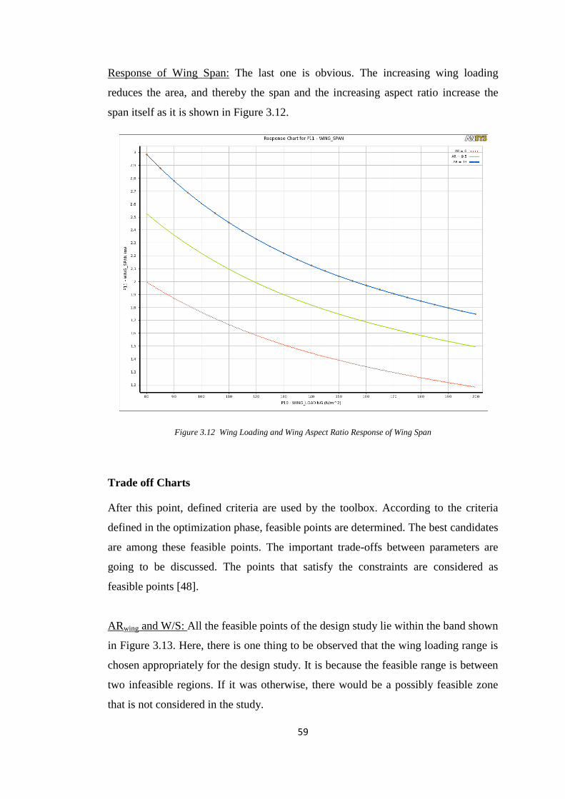
59

Response of Wing Span: The last one is obvious. The increasing wing loading

reduces the area, and thereby the span and the increasing aspect ratio increase the

span itself as it is shown in Figure 3.12.

Figure 3.12 Wing Loading and Wing Aspect Ratio Response of Wing Span

Trade off Charts

After this point, defined criteria are used by the toolbox. According to the criteria

defined in the optimization phase, feasible points are determined. The best candidates

are among these feasible points. The important trade-offs between parameters are

going to be discussed. The points that satisfy the constraints are considered as

feasible points [48].

ARwing and W/S: All the feasible points of the design study lie within the band shown

in Figure 3.13. Here, there is one thing to be observed that the wing loading range is

chosen appropriately for the design study. It is because the feasible range is between

two infeasible regions. If it was otherwise, there would be a possibly feasible zone

that is not considered in the study.

60

Figure 3.13 Trade-off Between W/S and AR_wing

W0 vs. E4: As shown in Figure 3.14, points with a total weight of above 5000 gr are

marked as infeasible. So, not all the points with high special mission endurance are

feasible due to the other requirements.

Stall Speed vs. E4: A narrow band is feasible for stall speed. Below 12.5 m/s, wing

loading is so low that the total weight requirement cannot be obtained. The points

having a stall speed higher than 14 m/s are also dismissed directly.

Stall Speed vs. W0: Together with Figure 3.14 and Figure 3.15, Figure 3.16 explains

the design limits very well. Above 14 m/s and the right side of 5000 gr are marked as

infeasible. In fact, these points are out of defined margins and not acceptable.

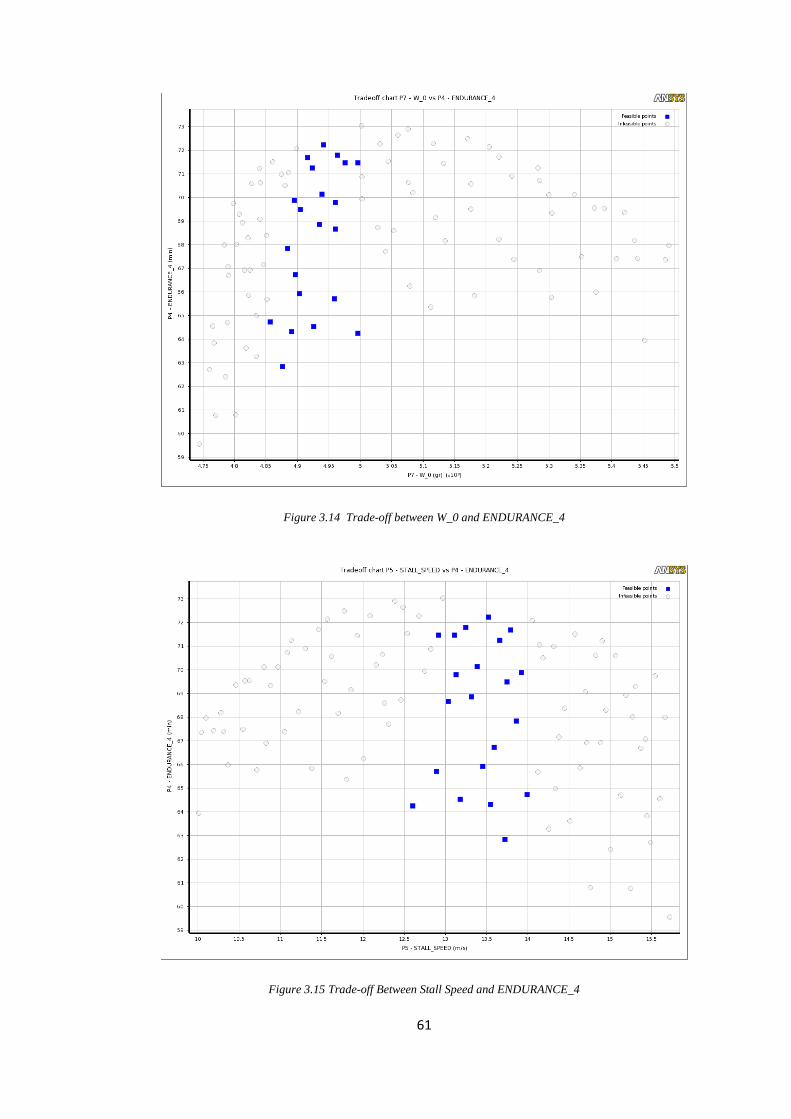
61

Figure 3.14 Trade-off between W_0 and ENDURANCE_4

Figure 3.15 Trade-off Between Stall Speed and ENDURANCE_4

62

Figure 3.16 Trade-off Between Stall Speed and W_0

Figure 3.17Trade-off Between The Wing Span and Aspect Ratio

63

Wing Span and Aspect Ratio: For each aspect ratio, there is a feasible wing span

zone. In fact this figure implies the same relationship with Figure 3.13, but from a

different point of view.

3.2 The Decision of the Final Design

In the light of all those charts and correlations, the final design is determined among

the candidates offered by the toolbox.

Figure 3.18The candidate Points

The stars next to the values show the goodness of the point in domain according to

the defined objectives. All the candidates have the best E4 values in domain as

expected. E1 has a similar requirement, so the same candidates also have the best E1

values in domain. On the other hand, it is understood that there are some candidates

have better E3 in domain but, they are not selected due to the priorities. In terms of

the total weight parameter, the candidates with moderate weights are found feasible.

The same observation is valid for the stall speed and the wing span.

For final decision, one of the candidates (the first one) is chosen to be the reference

and the variations of output parameters from the reference are examined.

64

Figure 3.19ENDURANCE_4 Values of the Candidates (units are in minutes)

As the primary consideration, the values of E4 are crucial. In Figure 3.19, only the

candidates 4 and 6 seem a bit lower than the reference.

Figure 3.20Design Take-off Weight Values of the Candidates (units are in grams)

For the design take-off weight, there is not an indicative difference between the

candidates. For stall speeds, Candidates 5, 7 and 8 seem better.

65

Figure 3.21Stall Speed Values of the Candidates (units are in m/s)

For the wing span, the values vary significantly. The candidates 4, 6 and 8 have

shorter wings, which could be advantageous for the final decision.

Figure 3.22Wing Span Values of the Candidates (units are in meters)

The quad-rotor mode endurance is almost the same for all candidates.

66


The horizontal flight endurances, E1, are well above the requirement, and they do not

vary significantly.

To sum up, all the candidates are well suited for the design requirements, so any of

them may be the final design choice. In overall, it is seen that the endurance values

do not vary significantly. In addition to that the stall speed and the total weight

values are very close to each other. The only indicative parameter remains is the

wing span. As explained before a relatively shorter wing is a reason for preference.

Additionally, considering the variations of the other parameters the final design point

is determined to be “Candidate Point 8”.


67

3.3 The Numerical Outputs

All the numerical values are calculated in MS Excel file by the embedded formulas,

which are given in the section, “Construction of the MS Excel File”.

Geometrical Outputs

Table 3.1 Geometrical Outputs

Fuselage Length (lfuselage) 0.82 m

Fuselage Diameter (dfuselage 0.14 m

Length of Motor Booms (lmotor boom) 0.6 m

Length of Tail Boom (ltail boom) 0.43 m

Wing Span (bwing) 1.821 m

Horizontal Tail Span (bht) 0.365 m

Vertical Tail Span (bvt) 0.252 m

Wing Root Chord (cr_wing) 0.245 m

Wing Mean Chord ( wing) 0.191 m

Wing Tip Chord (ct_wing) 0.123 m

Horizontal Tail Root Chord (cr_ht) 0.139 m

Horizontal Tail Mean Chord ( hg) 0.108 m

Horizontal Tail Tip Chord (ct_ht) 0.0695 m

Vertical Tail Root Chord (cr_vt) 0.210 m

Vertical Tail Mean Chord ( vt) 0.163 m

Vertical Tail Tip Chord (ct_vt) 0.105 m

Wing Reference Area (Sref_wing) 0.334 m2

Horizontal Tail Reference Area (Sref_ht) 0.0380 m2

Vertical Tail Reference Area (Sref_vt) 0.0400 m2

Angle of Incidence (AOI) 3.27°

68

Weight Outputs

Table 3.2 Weight Outputs

Fuselage Weight (Wfuselage) 448.9 gr

Fuselage Weight Including Motor Booms 526.2 gr

Wing Weight (Wwing) 476.3 gr

Horizontal Tail Weight (Wht) 48.1 gr

Vertical Tail Weight (Wvt) 50.8 gr

Empty Weight (We) 2464.2 gr

Design Take-off Gross Weight (W0) 4939.8 gr

Quad-rotor Weight (Wquad) 3886.6 gr

Aerodynamic and Performance Outputs

Table 3.3 Aerodynamic and Performance Outputs

Fuselage Parasite Drag Coefficient ( ) 0.00539

Wing Parasite Drag Coefficient ( ) 0.00541

Horizontal Tail Parasite Drag Coefficient

( )

0.000787

Vertical Parasite Drag Coefficient ( ) 0.000661

Motor Booms Normalized Drag

Coefficient( )

0.0252

Parasite Drag Coefficient ( ) 0.0393

Design Lift Coefficient (cL) 0.655

Design Drag Coefficient at Cruise (cD) 0.0576

69

Maximum Lift Coefficient ( ) 1.46

Oswald Span Efficiency (e) 0.760

K 0.0425

Lift Curve Slope ( ) 5.014 rad

-1

Power Required at Cruise (Pr) 152.1 W

Thrust Required at Cruise (Tr) 434.0 gf

Power Available (Pa) 1232 W

Mission 1 Endurance (E1) 101.9 min




Stall Speed (Vstall) 13.4 m/s

Maximum Rate of Climb (R/Cmax) 24.2 m/s

Maximum Speed (Vmax) 55.2 m/s

Maximum Load Factor (nmax) 7.65

Corner Velocity (V*) 37.1 m/s

Maximum Turn Rate (ωmax) 2.01 s-1

Minimum Turn Radius (Rmin) 18.4 m

Maximum Load Factor Variation with Velocity: nmax varying with velocity generates

the typical shape of the flight envelope as shown in Figure 3.25. The corner velocity

is the corresponding velocity where two limiting curves intersect.

Power Required and Power Available Variation with Velocity: The available power

is constant with velocity; and the required power increases exponentially after a

minimum. The maximum velocity is the corresponding velocity where two curves

intersect in Figure 3.26.

Table 3.3 (continued)

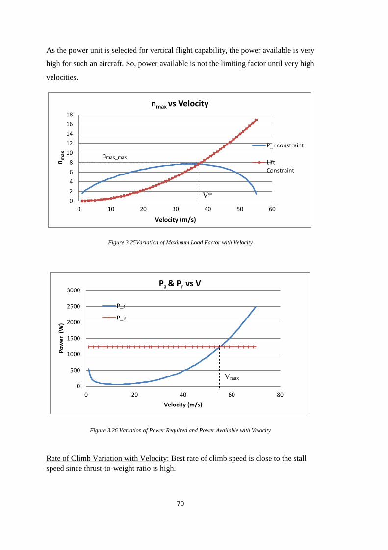
70

As the power unit is selected for vertical flight capability, the power available is very

high for such an aircraft. So, power available is not the limiting factor until very high

velocities.

Figure 3.25Variation of Maximum Load Factor with Velocity

Figure 3.26 Variation of Power Required and Power Available with Velocity

Rate of Climb Variation with Velocity: Best rate of climb speed is close to the stall

speed since thrust-to-weight ratio is high.

0

2

4

6

8

10

12

14

16

18

0 10 20 30 40 50 60

nm

ax

Velocity (m/s)

nmax vs Velocity

P_r constraint

LiftConstraint

0

500

1000

1500

2000

2500

3000

0 20 40 60 80

Po

we

r (

W)

Velocity (m/s)

Pa & Pr vs V

P_r

P_a

V*

nmax_max

Vmax

71

3.27Rate of Climb Variation with Velocity

3.4 Constructing the Outer Geometry

Many non-generic formulas shaping the outer geometry of the aircraft are generated

and modified according to the initial CAD drafts while constructing the mathematical

model. Therefore geometry outputs of the MS Excel file defines almost everything

regarding to the outer geometry. A basic methodology is followed in constructing the

outer geometry. The logical steps generating the geometry are the followings:

Fuselage

i. A cylindrical gimbal with known diameter is located on the front.

ii. A circular boom with known diameter is inserted at the back.

iii. The distance between them is known (output of the model).

iv. Between head and tip, two motor booms and one wing are located.

v. Considering the propeller clearances, their locations are more or less definite.

vi. A modular high wing, composed of right and left parts, is placed in its position,

so the curvature of the upside of the fuselage continues smoothly between two

parts in span-wise direction.

vii. The lofting of the fuselage surface is tangent to the wing’s airfoil’s upper

surface in chord-wise direction.

viii. Underside of the fuselage should be appropriate for landing on it.

0

5

10

15

20

25

30

0 10 20 30 40 50 60

R/C

(m

/s)

Velocity (m/s)

Rate of Climb vs V

72

ix. Sides are relatively flat especially the zones for the motor booms’ inserts.

Wing

i. After very rough static margin estimation the position of the wing is ensured

not to be too bad and fixed, and fuselage is modified accordingly.

ii. Airfoil is drawn at the symmetry axis, set the incidence angle with respect to

the fuselage, and swept through a straight line, which is perpendicular to the

symmetry axis, at the quarter chord until the wing tip with a known taper.

iii. The control surfaces are determined to have width of 30% of the local chord

and length of 70% of the span.

Booms

i. Ensure the locations of the motor booms.

ii. Draw the tail boom according to the predetermined length.

Tails

i. For vertical tail, the airfoil is drawn at the centric axis of the tail boom. Sweep

the profile from the trailing edge vertically up to the tail tip, which is at a

known distance. (As explained before due to the ease of manufacturing, the

sweeps at the trailing edges are zero for both tails.)

ii. Trim the vertical tail and generate a smooth surface transition for boom

junction.

iii. For horizontal tail, is drawn at the centric axis of the tail boom. Sweep the

profile in a same manner with the vertical tail. Trim the portion that the boom

is inserted and generate a smooth surface transition at the junction.

iv. The control surfaces are determined to have width of 25% of the mean chord

and length of 90% of the span.

73

Figure 3.28Isometric View of the Quad-rotor Mode of the Aircraft

Figure 3.29Isometric View of the Fixed Wing Mode of the Aircraft (Horizontal Flight Mode)

74

Figure 3.30 Isometric View of the Fixed Wing Mode of the Aircraft (Vertical Flight Mode)

In Figure 3.29 and Figure 3.30, isometric views of the aircraft, in horizontal and

vertical flight respectively, can be seen. This is the final outer geometry drawn

according to the logic written above; and this is the prototype to be manufactured. In

Figure 3.31, three views of the aircraft are shown. The curvatures of the aircraft can

be seen clearly there.

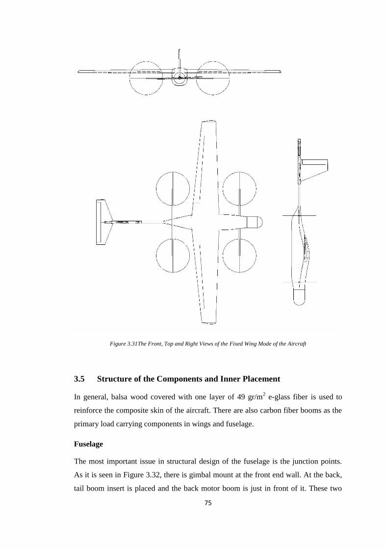
75

Figure 3.31The Front, Top and Right Views of the Fixed Wing Mode of the Aircraft

3.5 Structure of the Components and Inner Placement

In general, balsa wood covered with one layer of 49 gr/m2 e-glass fiber is used to

reinforce the composite skin of the aircraft. There are also carbon fiber booms as the

primary load carrying components in wings and fuselage.

Fuselage

The most important issue in structural design of the fuselage is the junction points.

As it is seen in Figure 3.32, there is gimbal mount at the front end wall. At the back,

tail boom insert is placed and the back motor boom is just in front of it. These two

76

booms are structurally integrated by using the balsa bulkheads. The front motor

boom is reinforced in similar fashion. Lastly the wing junction zone is supported

with balsa plates.

The main strategy here is to distribute the stress at that junction points. As it is

explained in the manufacturing chapter, extra honeycomb and carbon fiber layers are

added at that junction zones.

Wing

The inner structure of the wing is composed of the balsa ribs and carbon fiber tube

spars. At the root the ribs are more frequent and the tubes have larger diameter. As

shown in Figure 3.33, the front spar is composed of centric carbon fiber tubes with

decreasing diameter from root to tip. On the other hand, due to the geometry of the

wing, the rear spar cannot be a centric combination and split into three separate parts

again decreasing diameter from root to tip.

Figure 3.32Inner Structure of the Fuselage

77

Figure 3.33Inner Structure of the Wing

Horizontal and Vertical Tails

As shown in Figure 3.34 and Figure 3.35, e-glass coated balsa ribs and spars are

used in horizontal and vertical tails. There is no extra carbon tube in tail parts; but the

tail boom supports them. The spars are adhered to the tail boom in both tails.

Figure 3.34Inner Structure of the Horizontal Tail

78

Figure 3.35Inner Structure of the Vertical Tail

Placement inside the Fuselage

The placement of the wing is dependent on many other parameters and more or less

determined by the outputs of the optimization phase. So the placement of the inner

components are done in such a way that the center of gravity is in an appropriate

place with respect to the wing aerodynamic center. The center of gravity and the

static margin are calculated roughly in MS Excel file automatically by using the

parametric values of all variables like other geometric and performance outputs; and

an approximate value is found. This calculation is used in the wing geometry

construction step, which is mentioned above: “After very rough static margin

estimation the position of the wing is ensured not to be too bad and fixed, and

fuselage is modified accordingly.”

In the end, all the weights are defined in CAD program and the center of gravity is

checked accordingly.

For quad-rotor mode, center of gravity is aimed to be located at the middle of the

motor booms to balance the motors. Therefore, the extra battery is placed at the very

back of the fuselage.

79

Figure 3.36 Placement of the Components (Fixed Wing Mode)

Figure 3.37 Placement of the Components (Quad-rotor Mode)

3.6 Static Margin Calculation

For fixed wing mode, the static margin calculation is very crucial in terms of

understanding the characteristics of the longitudinal stability of the aircraft.

According to the final placement and CAD drawings, the weight distribution is

finalized. The static margin calculations are done according to [49].

The parameter is the normalized (by wing mean chord) value of the location of

the center of gravity of the aircraft on body-x axis in stability coordinate system. It is

found by simply adding up all the components in Table 3.4.

ESC Video Modem

Antenna

ESC

Avionic Box

Brushless DC Motor Tilt Mechanism

Battery 1 AGL Sensor

Battery 2

80

Table 3.4 Weight Distribution of the Fixed Wing Mode

Component Weight (gr) X

(mm)

Fuselage 448.9 351.7

Wing 476.3 458.7

Horizontal Tail 48.1 1.291

Vertical Tail 50.8 1084

Tail Boom 35.5 1033

Motor Booms 77.3 491.6

Motors 520 491.6

ESC’S 144 389.7

Avionic Box 212 450.1

Tilt Mechanisms 324 491.6

Battery 1’s 1422 545.8

Battery 2 250 450.8

Payload 700 70*

Antenna 36 180.8

Video Modem 70 310.5

AGL Sensor 50 458.7

Cables 74.9 520.6

TOTAL (gr) / Xcg

(mm)

4939.8 437.7

(

According to the final placement,

and

81

The contribution of the fuselage to the pitching moment is as follows,

, according to the figure in [REF 49].

The tail dynamic pressure ratio,

, where √

Downwash:

[ √ ( ]

The value of the static margin is 7.58 %, and it is between the margins of 5-10%,

which is typical for that kind of a plane [40].

83

CHAPTER 4

4. MANUFACTURING

Manufacturing of the prototype is long and demanding work. It is a process from

drawing the spline of the airfoil to painting of the body. The steps of the

manufacturing are shown in Figure 4.2.

4.1 Constructing a Manufacturable Geometry

Carrying the Numerical Values of the Design Output to the CAD

The drawing of the outer geometry of the aircraft starts with the coordinates of the

wing airfoil. The spline of SD7062 airfoil is discretizated by 100 points. The

coordinates of the points are scaled according to the root chord length of the aircraft.

After that the wing geometry is drawn according to the span, taper and sweep values.

The same methodology is applied for the tail surfaces. In Figure 4.1, the root and tip

chord, quarter-chord-line that has no sweep and the root chord line tilted according to

the set angle of the wing can be seen. The wing surface is generated by sweeping the

tapered airfoil spline between root and chord.

Figure 4.1Construction of the Wing Surface

84

Figure 4.2Manufacturing Steps

Numerical values from the geometrical outputs of the conceptual design

Constructing the outer geometry according to the physical concept of the aircraft and design of the inner structure

Splitting the whole geometry into the parts that can be manufactured by seperate molds (Left wing upper surface,

fuselage right surface etc.)

Drawing female molds of the seperate parts, which can be manufactured by 3-axis CNC machine; and inner structure

frames which can be manufactured by laser cut

Constructing feasible toolpaths and NC codes for the molds

Machining the molds

Applying appropriate surface finish treatments for composite production

Production of the composite skin and inner stucture frames

Installation of the wiring ; and adhering the inner structure parts and surface pairs together

Surface Finish Treatments and painting

Installation of the equipments (motors, propellers etc.)

Constructing the Geometry According to the Physical Concept of

the Aircraft

85

For the fuselage, the locations of the wing and motor booms are critical. The length

and diameters are directly taken from the design outputs. The upper surface of the

wing airfoil is used to shape the upper part of the fuselage. To bottom line of the

fuselage is drawn considering that there is not landing equipment and the aircraft

directly lands on its fuselage. The side of the fuselage is drawn considering that the

wing is mounted on the sides. In general, guiding lines and the reference cross-

sections have smooth transitions to obtain an aerodynamically efficient body.

Figure 4.3Guiding Curves and Reference Cross-Sections of the Fuselage

Splitting the Geometry and Drawing the Female Molds

Because this is an aircraft and the outside of the surfaces are interacted with air; the

outside of the skin parts are supposed to be smooth and shiny considering the surface

roughness and drag issues. The side that is faced to the mold becomes shiny in

composite manufacturing; therefore, female molds are used.

The molds are machined by a 3-axis CNC machine. The knife of the machine is

perpendicular to the log; and it machines the log from one direction only. Therefore,

adverse slopes in the mold geometries cannot be machined and they are not allowed.

86

To illustrate, in Figure 4.4, the portion above the dashed line has an adverse slope

and that zone cannot be machined. Primary thing to consider when splitting the

geometry is not to have adverse slope. So the outer geometry is split from the

extremum points. And when the outer geometry is crated, it is taken into account not

to have more than one local extremum lines on surfaces anyway.

The mounting points of the wing parts and the motor booms are determined on the

fuselage to ease the orientation and to avoid asymmetry problems as seen in

Figure 4.5. On the lower surfaces of the wing parts and horizontal tail, and on the

right side of the vertical tail, there are servo motor mounting zones fixed on the

molds.

There are ten molds produced:

- 2 for right and left fuselage surfaces

- 4 for upper and lower surfaces of the left and right wings

- 2 for upper and lower horizontal tail surfaces

- 2 for right and left vertical tail surfaces

The direction of the tool

Adverse Slope

Mold

Figure 4.4 An Example of Adverse Slope on Molds

87

Figure 4.5 CAD Drawing of the Molds (one side only)

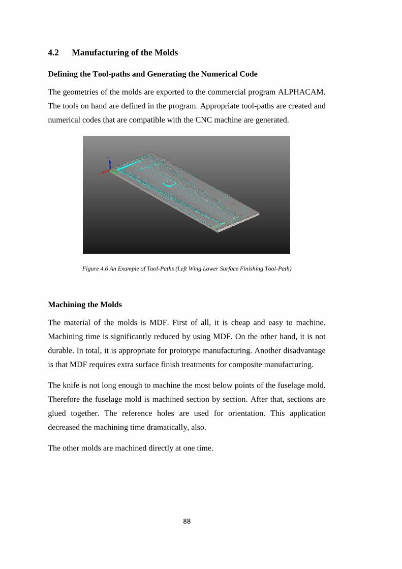
88

4.2 Manufacturing of the Molds

Defining the Tool-paths and Generating the Numerical Code

The geometries of the molds are exported to the commercial program ALPHACAM.

The tools on hand are defined in the program. Appropriate tool-paths are created and

numerical codes that are compatible with the CNC machine are generated.

Figure 4.6 An Example of Tool-Paths (Left Wing Lower Surface Finishing Tool-Path)

Machining the Molds

The material of the molds is MDF. First of all, it is cheap and easy to machine.

Machining time is significantly reduced by using MDF. On the other hand, it is not

durable. In total, it is appropriate for prototype manufacturing. Another disadvantage

is that MDF requires extra surface finish treatments for composite manufacturing.

The knife is not long enough to machine the most below points of the fuselage mold.

Therefore the fuselage mold is machined section by section. After that, sections are

glued together. The reference holes are used for orientation. This application

decreased the machining time dramatically, also.

The other molds are machined directly at one time.

89

Figure 4.7 Machining the Fuselage Mold

Figure 4.8 Scenes from Machining of the Molds (Finishing of the wing and horizontal tail; roughening of the

vertical tail)

90

Surface Finish Treatments

MDF soaks liquids if there is no coating on surface. So, it is not possible to apply

epoxy for manufacturing; and carrying on the procedure without sealing the surface

simply sticks the composite laminate to the mold. There are possible alternatives for

coating surface. For fuselage molds, at first, polyester putty is applied to surface.

After that, one layer of surfacing primer is used. Finally, two layers of varnish are

applied. Sanding is applied between all layers in a fining fashion. For other molds

polyester putty is not applied, and the rest is the same. Both brush and spray gun are

used in coating process.

Figure 4.9 Scenes from Surface Finishing Treatments (Polyester putty on fuselage mold, applying primer on wing

molds and varnished molds)

91

4.3 Manufacturing of the Composite Skins and Inner Structural

Frames

Methodology

In composite manufacturing, vacuum bagging wet lay-up method is used. This is a

typical procedure for homemade composite applications. MOMENTIVE (HEXION)

MGS L285 two component epoxy [50] is used as the resin, which is typical for small

scale aviation applications.

In wet lay-up, the operator simply drapes the plies onto the waxed molds and make

sure that the fabrics are impregnated well. The mixture of the resin, the amount of

used resin and the checking of the impregnation are directly dependent to the skill of

the operator. After draping, to hold the laminate in its position on the molds, it is

bagged and applied vacuum. The bagging is very crucial in terms of obtaining good

geometry. It is a simple composite manufacturing procedure with its pros and cons.

No heat treatment while curing is applied due to the lack of equipment.

The laminates of the composite skins are as shown in Figure 2.6, Figure 2.8 and

Figure 2.7.

Procedure of lay-up is as follows:

- Mold release agent is applied properly to the mold.

- Laminate is laid on the mold. At necessary zones, where the mold has corners

and other complexities; glass bubble or yarns of fabric are placed to hold the

resin at those points.

- Peel-ply film is not used due to the weight considerations; also the thicknesses of

the skins are very small, and the skin may be harmed while releasing the peel-

ply film. The surfaces to be adhered somewhere is going to be sanded

- Release film is laid and the bleeder is put onto it.

- All of them are put into the vacuum bag, sealant is checked; and vacuum is

applied.

- Wait for at least eight hours for curing.

After curing, parts are trimmed according to the contours on the molds.

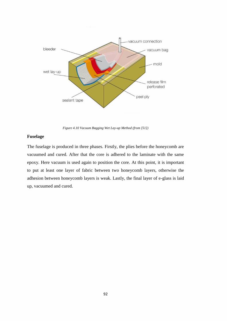
92

Figure 4.10 Vacuum Bagging Wet Lay-up Method (from [51])

Fuselage

The fuselage is produced in three phases. Firstly, the plies before the honeycomb are

vacuumed and cured. After that the core is adhered to the laminate with the same

epoxy. Here vacuum is used again to position the core. At this point, it is important

to put at least one layer of fabric between two honeycomb layers, otherwise the

adhesion between honeycomb layers is weak. Lastly, the final layer of e-glass is laid

up, vacuumed and cured.

93

Figure 4.11Manufacturing of the Fuselage Skins

94

Wing and Tail

The wing and tail surfaces are produced at one vacuum.

Figure 4.12Manufacturing of the Wing Skins

95

Figure 4.13 All of the Composite Skins Parts of the Aircraft

Inner Structural Frames

Inner structural frames are made of 2.5 mm coated with 49 gr/m2 e-glass fiber. A

plate is produced and the parts are obtained from it by laser cut.

Figure 4.14 Manufacturing of the Inner Structural Frames

96

Weights of the Produced Parts

After trimming the parts are weighed and compared with the weight estimation

outputs of the mathematical model.

(

Table 4.1 Comparison of the Calculated and Measured Weights of the Composite Skin Parts

Parts

Calculated Output of the MS EXCEL

(gr)

Measured Weight of the Produced

Part (gr)

Error (%)

Left Fuselage Surface 197.9

100 199 0.55

Right Fuselage Surface 99

Left Wing Upper Surface

236.1

58

222 -6.35 Left Wing Lower Surface 57

Right Wing Upper Surface 53

Right Wing Lower Surface 54

Horizontal Tail Upper Surface 35.2

19 38 7.37

Horizontal Tail Lower Surface 19

Vertical Tail Left Surface 37.9

17 38 0.26

Vertical Tail Right Surface 21

4.4 Assemblage

Fuselage

The inner structural frames and booms are adhered according to the CAD drawings

by using polyurethane and epoxy adhesives.

97

Figure 4.15Assemblage Steps of the Fuselage

Lastly two sides of the fuselage are brought together and adhered with a

polyurethane adhesive. This step is very critical as the symmetry of the aircraft is

crucial in terms of flight stability.

98

Figure 4.16 Assembled Fuselage

Wing

Firstly, the carbon fiber tubes serving as front spar are assembled. As the wing is

tapered, the diameters of the tubes reduce step by step. These tubes are adhered

together.

Figure 4.17 Front Spar of the Wing

All the ribs and spars are adhered together inside the mold, and then the assembled

inner structure is adhered to the upper surface of the wing. After that balsa laths are

adhered between ribs along the wing periphery to obtain a better adhesion surface

between upper and lower wing surfaces.

99

Figure 4.18Preparing the Upper Wing Surface

After that, lower surface adhered to the upper surface.

Figure 4.19Assembled Wings

100

Tails

Again, the inner structural frames are place on one side of the tail surfaces. The spars

are fixed such that they are in contact with the tail boom.

Figure 4.20 Inner Structure of the Tail Surfaces

At first, lower surface of the horizontal tail is adhered to the end of the tail boom, and

then the upper surface is placed on to the boom and the lower surface.

Figure 4.21 Horizontal Tail Adhered to the End of the Tail Boom

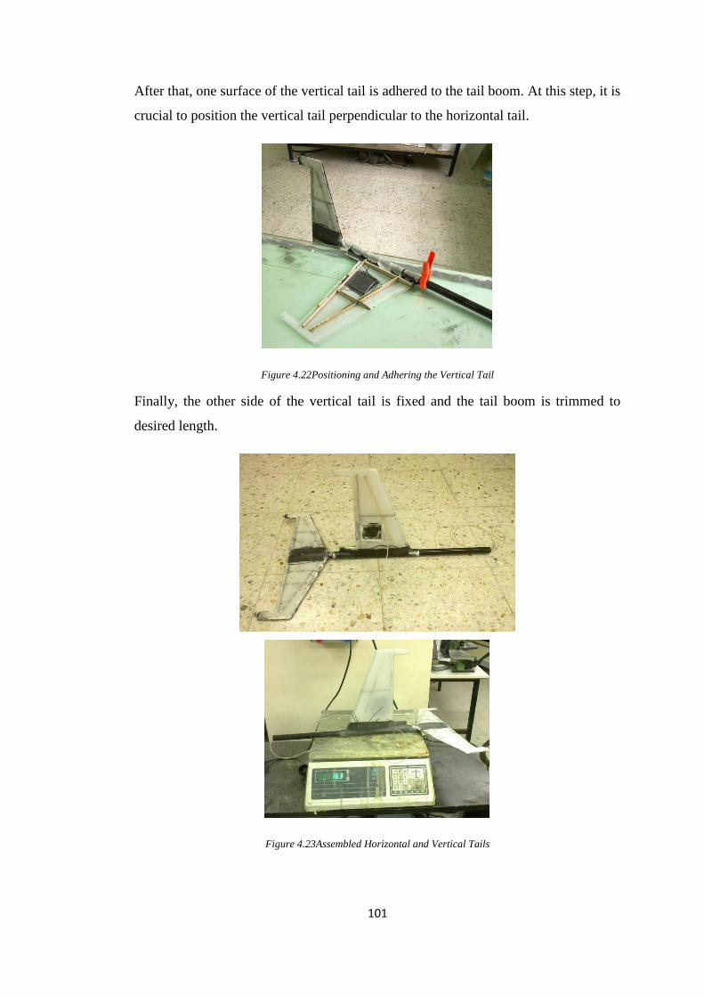
101

After that, one surface of the vertical tail is adhered to the tail boom. At this step, it is

crucial to position the vertical tail perpendicular to the horizontal tail.

Figure 4.22Positioning and Adhering the Vertical Tail

Finally, the other side of the vertical tail is fixed and the tail boom is trimmed to

desired length.

Figure 4.23Assembled Horizontal and Vertical Tails

102

Weights of the Assembled Parts

Overall production procedure highly depends on craftsmanship, so it is very difficult

to estimate the weights of the produced parts. Many components like wooden frames

or metal parts have certain weights. On the other hand, the weights of the composite

skins may change significantly due to the wrong mass ratio of fiber and resin. In wet

lay-up method, this ratio is completely dependent to the skill of the operator. In

addition to that, the amount of adhesive to be used is more ambiguous. In

mathematical weight model, the adhesive to be used is tried to be estimated

parametrically by taking every possible details into account. Despite that, the amount

of used adhesive creates a considerable difference between the calculated and

measured weight values.

In fuselage, all the internal frames are adhered to the skin and the amount of adhesive

to be used is calculated by an empiric formula depending on initial CAD drawings.

An allowable error is seen due to the fact that the shapes of the internal frames are

not determined beforehand and correlation between the fuselage dimensions and the

amount of adhesive to be used is not very strong.

In wings, the geometry is fairly determined and the regions to apply adhesive are

clear. The weights of the ribs and spars are calculated parametrically from the unit

weights. Therefore, the weight estimation seems more successful.

In tail parts, it is seen that the amount of adhesive needed to fix the tail boom to the

tail surfaces is much more than estimated. Also a more careful workmanship is

required at that phase comparing the other parts. As a result, the tail is produced a bit

heavier.

In overall, the estimated and calculated weight values are close enough to carry on

system development procedure. Approaching the problem in system level, it is

important to be aware that the requirements of the air vehicle may slightly change

during the development procedure, because of the external factors like a vibration

issue for the payload or shadowing problem for data-link antenna. These kinds of

troubles may result in additional weights to be loaded on the aircraft. After all,

system development is always an iterative procedure. So the weight of the prototype

is hardly possible to be the same with the final product. Here the important thing is to

103

show that it is possible to produce a useable prototype satisfying the basic

requirements like aerodynamical efficiency, structural integrity and physical space

for payloads.

Table 4.2 Comparison of the Calculated and Measured Weights of the Assembled Parts

Parts

Calculated Output

of the MS EXCEL

(gr)

Measured Weight

of the Produced

Part (gr)

Error (%)

Fuselage (with motor booms) 526.2 486 -8.27

Wing 476.3 470 -1.34

Tail (with tail boom) 134.4 163 17.5

TOTAL 1136.9 1119 -1.60

(

As explained in “Weight Estimation Parameters” part of Chapter 2, for standard

production of such an aircraft, the painting is planned to be done by injecting color

pigments into the resin. So, when the weight comparisons are made, unpainted state

of the prototype is used by considering that adding pigments have little contribution

to the total weight.

After the assemblage of the parts, the aircraft is ready to be installed other equipment

after the manufacturing process.

104

Figure 4.24Views of the Assembled Aircraft

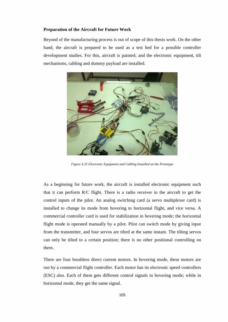
105

Preparation of the Aircraft for Future Work

Beyond of the manufacturing process is out of scope of this thesis work. On the other

hand, the aircraft is prepared to be used as a test bed for a possible controller

development studies. For this, aircraft is painted; and the electronic equipment, tilt

mechanisms, cabling and dummy payload are installed.

Figure 4.25 Electronic Equipment and Cabling Installed on the Prototype

As a beginning for future work, the aircraft is installed electronic equipment such

that it can perform R/C flight. There is a radio receiver in the aircraft to get the

control inputs of the pilot. An analog switching card (a servo multiplexer card) is

installed to change its mode from hovering to horizontal flight, and vice versa. A

commercial controller card is used for stabilization in hovering mode; the horizontal

flight mode is operated manually by a pilot. Pilot can switch mode by giving input

from the transmitter, and four servos are tilted at the same instant. The tilting servos

can only be tilted to a certain position; there is no other positional controlling on

them.

There are four brushless direct current motors. In hovering mode, these motors are

run by a commercial flight controller. Each motor has its electronic speed controllers

(ESC) also. Each of them gets different control signals in hovering mode; while in

horizontal mode, they get the same signal.

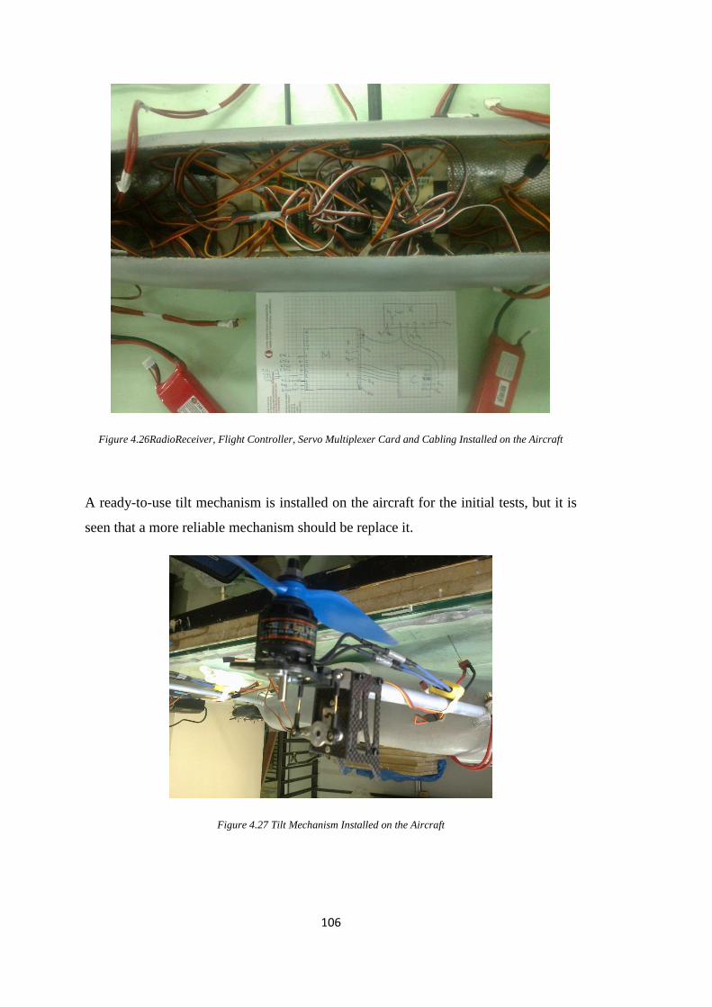
106

Figure 4.26RadioReceiver, Flight Controller, Servo Multiplexer Card and Cabling Installed on the Aircraft

A ready-to-use tilt mechanism is installed on the aircraft for the initial tests, but it is

seen that a more reliable mechanism should be replace it.

Figure 4.27 Tilt Mechanism Installed on the Aircraft

107

Figure 4.28 View of the Equipped Aircraft (Fixed Wing Mode)for R/C Flight

Figure 4.29 View of the Equipped Aircraft (in Quad-rotor mode) for R/C Flight

108

Figure 4.30 A Scene From Vertical Flight in Quad-rotor Mode

As it is stated some flight tests are conducted only to get an idea about the future

work on mechanical side (tilt mechanism, vibration etc.), and no data is collected

during these tests.

109

CHAPTER 5

5. CONCLUSION

In this thesis study, optimal design and prototype manufacturing procedures of a

miniature class convertible quad tilt rotor (QTR) unmanned air vehicle (UAV) are

explained. The aircraft carries its four motors on its motor booms separately from the

wing. These four motors can be tilted to change the flight mode of the aircraft from

horizontal to vertical flight, and vice versa. This design choice gives the aircraft the

capability of operating as a fixed wing aircraft and a quad-rotor optionally. The

modular design of the aircraft enables the operator to demount the wing and tail parts

to use the aircraft as a highly manoeuvrable quad-rotor with tilting rotors. The fixed

wing mode of the aircraft has VTOL capabilities, and a combined flight endurance of

about 70 minutes. The combined flight refers to total 5 minutes of hovering,

excluding vertical take-off and landing, besides horizontal flight. This ability of

flight mode transition gives aircraft mission flexibility in many areas. The quad-rotor

mode has almost 30 minutes of hovering time. In quad-rotor mode, an extra battery

module can be installed instead of the removed wing and tail parts to extend the

flight time. The motivation behind the optional quad-rotor mode is to obtain stealth

and longer hovering time for some special mission objectives. The payload of the

aircraft is a gyro stabilised gimbal with electro-optical day light and infrared sensors,

which weighs about 700 grams.

Inherently, the primary objectives of the aircraft are accomplishing intelligence,

surveillance and reconnaissance missions. Therefore the design procedure is

conducted such that the primary consideration is maximizing the endurances of the

determined mission profiles. Besides, the introduced conceptual design methodology

can be used to maximize the payload weight or maximum velocity of the aircraft as

well. Almost no modification in mathematical model is required to accomplish

completely different optimization cases.

110

The main claim of this thesis study is to show the applicability of MS Excel-Ansys

Workbench Design Optimization Toolbox coupled design methodology for such an

aircraft design study. In this optimal design procedure, firstly a numerical model, in

which all the weight estimation, outer geometry and performance parameters are

calculated iteratively by embedded generic and non-generic formulas, is constructed

in MS Excel. Then this model is introduced to Ansys Workbench’s Design

Optimization Toolbox. All the characteristics of the mathematical model are

examined in detail by local sensitivity curves, response curves and trade-off charts.

According to the requirements of the aircraft, the best candidates are determined by

the toolbox from the pool of design cases that are created by using the mathematical

model. Multi-objective genetic algorithm (MOGA) is used in the optimization phase,

which is found to be most appropriate for this design study. For instance, MOGA

allows multiple objectives like maximizing the combined flight endurance, limiting

the total weight and minimizing stall speed at the same time according to the tuned

priorities.

After the optimization procedure, a set of design parameters, including all

geometrical and performance outputs, is obtained. According to these outputs, the

outer geometry and inner structure of the aircraft is drawn. The molds for

manufacturing the aircraft are designed. Tool-paths and numerical codes to machine

the molds are constructed, and 10 parts of molds are machined by a 3-axis CNC

machine. Surface finishing treatments are applied to the molds, so that they are

prepared for wet lay-up composite production. The skin of the aircraft is made of

composite materials, namely e-glass fiber, carbon fiber, aramid (Kevlar) fiber,

Rohacell® foam, aramid honeycomb and epoxy resin. The measured weights of the

manufactured composite skins and calculated values of them are compared; and it is

seen that the estimation of the mathematical model is satisfactory. In inner structure

of the aircraft, e-glass coated balsa frames and carbon fiber tubes are used. In

assembly phase, the inner components and composite skins are adhered. Assembled

parts’ values are also measured and compared with the calculated values; and the

errors are found to be acceptable. Considering that all the other electronic

components of the aircraft are ready-to-use equipment, whose weights are well

known; the weight estimation of the mathematical model is proven to be functional.

111

Consequently, it is seen that by coupling MS Excel and Ansys Workbench’s Design

Optimization Toolbox, an optimal output can be obtained for defined set of

requirements. In addition to that, the estimations of the mathematical model are

accurate enough such that the weight of the manufactured prototype is very close to

the calculated value. The prototype is ready to be installed payload, mechanisms,

motors, and electronic equipment.

Justifications of the aerodynamic and structural designs are made. It is possible and

straightforward to implement the result of CFD runs to the optimization procedure,

but it increases calculation costs enormously. So, CFD analyses are used to check the

design. CFD analyses are conducted to calculate the critical aerodynamic properties

of the aircraft. The outcomes of the CFD runs are compared with the results of the

analytical calculations made by the mathematical model used in the design study.

Static loading tests are applied to the wing and the motor booms of the aircraft.

Elliptical wing loading is assumed for wing loading and 1g and 3g loading cases are

tested. No sign of fracture or surface buckling is observed.

Possible solutions for drag problem of the motor booms in horizontal flight are

discussed. This is the fundamental problem of the concept. Due to the circular

cylinder shape of the motor booms, form drag of them in horizontal flight is very

high. There are very obvious improvements for this issue, but finding an optimal

solution is very hard and complicated work considering all the dynamics of the

system. So for this thesis study, CFD solutions are used to comment on the issue and

the possible solutions are discussed; but the base (reference) case -booms with

circular cylinder shape- is kept in design phase.

As future work, the suggested items are the followings:

- The mode transition of the aircraft should be studied in detail. Thrust data of

the propulsion unit should be collected at different angles and speeds of the heading

wind. The test should be employed statically, and, if possible, dynamically by using a

tilt mechanism. The best way for mode transition in terms of propulsion should be

investigated.

112

- A mathematical flight model should be constructed by using motor tests’ and

CFD data. Guidance algorithms for efficient flight and mode transition should be

generated by using this model.

- By employing an inertial measurement unit (IMU), flight test should be

conducted and sets of data should be collected for validating the mathematical flight

model.

- A genuine autopilot system specific for this aircraft should be developed by

integrating attitude control, guidance and navigation algorithms.

- Data-link and video-link tests should be conducted and verified.

- Vibration analysis for the aircraft and refinement for tilt mechanism should be

performed.

- For motor booms, drag reduction studies should be conducted.

- Stability and performance of the tailless version of this aircraft concept in

horizontal flight should be investigated by using the mathematical models. By

driving the tilting servos and propulsive motors separately, the need for tail can be

eliminated. So a significant decreasing in total weight can be obtained.

113

REFERENCES

[1]. Bell X-22, Retrieved in July 2014, “http://en.wikipedia.org/wiki/Bell_X-22”.

[2]. Bell Boeing Quad Tilt Rotor, Retrieved in July 2014,

“http://en.wikipedia.org/wiki/Bell_Boeing_Quad_TiltRotor”.

[3]. Gupta, V., “Quad Tilt Rotor Simulations in Helicopter Mode using

Computational Fluid Dynamics” Ph.D. Thesis, University of Maryland,

College Park, 2005.

[4]. Armutçuoğlu, Ö., “The Conceptual Design Of a Tilt-Duct VTOL UAV” M.Sc.

Thesis, Middle East Technical University, December 2000.

[5]. Bell Boeing V-22 Osprey, Retrieved in July 2014,

“http://www.boeing.com/boeing/rotorcraft/military/v22”.

[6]. Agusta Westland AW609, Retrieved in July 2014,

“http://www.agustawestland.com/product/aw609”.

[7]. Boeing Phantom Swift, Retrieved in July 2014,

“http://www.boeing.com/boeing/Features/2013/09/bds_phantom_swift_09_11_

13.page”.

[8]. Bell Eagle Eye, Retrieved in July 2014,

“http://en.wikipedia.org/wiki/Bell_Eagle_Eye”.

[9]. IAI Panther, Retrieved in July 2014, “http://www.iai.co.il/2013/35673-41636-

en/IAI.aspx”.

[10]. KARI Smart UAV, Retrieved in July 2014,

“http://www.uasvision.com/2011/12/01/south-korea-tilt-rotor-uas”.

[11]. Ozdemir, U. et al, “Design of a Commercial Hybrid VTOL UAV System” ,

Journal of Intelligent and Robotic Systems, Volume 74, Issue 1-2, Pages 371-

393, April 2014.

[12]. Koker 1, Retrieved in July 2014, “http://theaviationist.com/2012/11/08/koker”.

[13]. IAI Mini Panther, Retrieved in July 2014, “http://www.iai.co.il/2013/35673-

41637-en/IAI.aspx”.

[14]. Cetinsoy, E. et al, “Design and construction of a novel quad tilt-wing UAV”,

Mechatronics, Volume 22, Issue 6, Pages 723–745, September 2012.

http://en.wikipedia.org/wiki/Bell_X-22

114

[15]. Flores, G., Escareño, J., Lozano, R., Salazar, S., “Four Tilting Rotor

Convertible MAV: Modeling, Control and Real-time Hover Flight Control”,

Journal of Intelligent & Robotic Systems, Volume 65, Issue 1-4, Pages 457-

471, January 2012.

[16]. Aerovironment Shrike VTOL, Retrireved in July 2014,

“https://www.avinc.com/uas/adc/shrikevtol”.

[17]. IAI Ghost, Retrieved in July 2014, “http://www.iai.co.il/36079-43473-

en/BusinessAreas_UnmannedAirSystems.aspx”.

[18]. IAI Bird Eye 500, Retrieved in July 2014,

“http://www.unmanned.co.uk/autonomous-unmanned-vehicles/uav-data-

specifications-fact-sheets/bird-eye-500-unmanned-vehicle-uav-specifications-

data-sheet”.

[19]. Aerovironment RQ-11B Raven, Retrieved in July 2014,

“http://www.avinc.com/uas/small_uas/raven”.

[20]. Aerovironment RQ-20A Puma, Retrieved in July 2014,

“http://www.avinc.com/uas/small_uas/puma”.

[21]. EMT Aladin, Retrieved in July 2014,

“http://en.wikipedia.org/wiki/EMT_Aladin”.

[22]. Aeronautics Orbiter, Retrieved in July 2014, “http://www.aeronautics-

sys.com/orbiter_mini_uav_muas”.

[23]. Rafael Skylite B, Retrieved in July 2014,

“http://www.rafael.co.il/Marketing/334-919-en/Marketing.aspx”.

[24]. IAI Bird Eye 400, Retrieved in July 2014, “http://www.iai.co.il/35098-34720-

en/Groups_Military_Aircraft_MALAT_Products_Bird_Eye_Family.aspx”.

[25]. Topivision Casper 200, Retrieved in July 2014, “http://defense-

update.com/products/c/casper200.htm”.

[26]. DP-6 Whisperer, Retrieved in July 2014,

“http://dragonflypictures.com/index.php?option=com_content&task=view&id=

15”.

[27]. Heli Spy II, Retrieved in July 2014, “http://www.unmanned.co.uk/autonomous-

unmanned-vehicles/uav-data-specifications-fact-sheets/helispy-ii-unmanned-

vehicle-uav-specifications-data-sheet”.

115

[28]. Datron Scout, Retrieved in July 2014, “http://www.dtwc.com/products/aerial-

recon/scout-suas”.

[29]. Honeywell RQ-16 T-Hawk, Retrieved in July 2014,

“http://en.wikipedia.org/wiki/Honeywell_RQ-16_T-Hawk”.

[30]. Oviwun, Retrieved in July 2014,

“http://www.trekaero.com/Trek_VTOL_OVIWUN_Specifications.htm”.

[31]. Uavvision Gyro-Stabilized Multi-Sensor CM100 Gimbal, Retrieved in July

2014, “http://www.uavvision.com/product/cm100-html”.

[32]. City Center Altitudes in Turkey, Retrieved in July 2014,

“http://tr.wikipedia.org/wiki/T%C3%BCrkiye_il_merkez_rak%C4%B1mlar%

C4%B1”

[33]. Cloud Cap Piccolo Nano Autopilot, Retrieved in July 2014,

“http://www.uasvision.com/2013/03/22/cloud-cap-technology-launches-

piccolo-nano-autopilot-for-small-uas”.

[34]. TP-Link Omni Antenna, Retrieved in July 2014, “http://www.tp-

link.com/en/products/details/?model=TL-ANT2415D”.

[35]. UTC Aerospace Systems AGL Sensor, Retrieved in July 2014,

“www.cloudcaptech.com/Sales%20and%20Marketing%20Documents/AGL%2

0Sensors%20Data%20Sheet.pdf”

[36]. TP-Link Video-link, Retrieved in July 2014, “http://www.tp-

link.com/lk/products/details/?model=TL-WA5210G”

[37]. Thunder Power Lithium Polymer Battery 8000mAh 3-CELL/3S4P 11.1V PRO

LITE MS LIPO, Retrieved in July 2014,

“http://www.thunderpowerrc.com/Products/8000-mAh_2/TP8000-3S4PL”.

[38]. Thunder Power Lithium Polymer Battery 3300mAh 3-Cell/3S 11.1V G8 Pro

Lite+ 25C LiPo, Retrieved in July 2014,

“http://www.thunderpowerrc.com/Products/3300-mAh_3/TP3300-3SPP25”.

[39]. PT-326 Polyurethane Structural Adhesive, Retrieved in July 2014,

“www.easycomposites.co.uk/downloads/TDS/EC-TDS-PT326.pdf”

[40]. Raymer, Daniel P., Aircraft Design: A conceptual Approach, AIAA, 1992.

[41]. Airfoil Database, Retrieved in July 2014, “http://airfoiltools.com”

116

[42]. Scorpion SII-3014-830KV (V2), Retrieved in July 2014,

“http://www.scorpionsystem.com/catalog/motors/s30_series_v2/SII-3014-

830KV”.

[43]. Roskam, Jan , Airplane Flight Dynamics And Automatic Flight Controls,

Roskam Aviation and Engineering Corporation, 1979.

[44]. Roskam, Jan , Tau Edward Lan, Dr. Chuan, Airplane Aerodynamics and

Performance, DarCorporation, 1997.

[45]. Hoerner, S. F., Fluid-Dynamic Drag, Hoerner Fluid Dynamics, 1965.

[46]. Anderson, John D., Aircraft Performance and Design, McGraw-Hill, 1999

[47]. Kacar, A., Üç Dönerkanatlı ve Döner-Rotorlu İnsansız Hava Aracının

Tasarımı, EMO, Cilt 3, Sayı 6, 2014.

[48]. Ansys Workbench User’s Guide Release 15.0, Nov 2013

[49]. Roskam, Jan, Methods for Estimating Stability and Control Derivatives of

Conventional Subsonic Airplanes, 1971.

[50]. MGS Epoxy L285/H285, Retrieved in July 2014, “http://www.kompozit.net”.

[51]. Vacuum Bagging Wet Lay-up Method, Retrieved in July 2014,

“http://www.kutec.at/vakuum.html”.

[52]. R. H. Stone, “Control Architecture for a Tail-sitter Unmanned Air Vehicle”,

5th Asian Control Conference, Melbourne, Australia, July 23-25, 2004.

[53]. D. Snyder, “The Quad Tiltrotor: Its Beginning and Evolution”, Proceedings of

the 56th Annual Forum, American Helicopter Society, Virginia Beach,

Virginia, May 2000

[54]. W. E. Green and P. Y. Oh, “Autonomous Hovering of a Fixed-Wing Micro Air

Vehicle”, International Conference on Robotics and Automation, Orlando,

Florida, USA, May, 2006

[55]. Radhakrishnan, A., Schmitz, F., “Quad Tilt Rotor Download and Power

Measurements in Ground Effect,” Proceedings of the 24th Applied

Aerodynamics Conference, AIAA, San Francisco, CA, June 2006.

[56]. Etkin, Bernard, Dynamics of Atmospheric Flight, 1972.

[57]. Science Fair Projects, Retrieved in August 2014,

“http://www.sciencebuddies.org/science-fair-

projects/project_ideas/Sports_p012.shtml”.

117

[58]. Choi J, Jeon WP, Choia H. “Mechanism of Drag Reduction by Dimples on a

Sphere.” Physics of Fluids. Vol.18 4 041702. 2006.

[59]. Tsutsui, T., Igarashi, T., “Drag Reduction of a Circular Cylinder in an Air-

stream”, Journal of Wind Engineering and Industrial Aerodynamics, 90, 527-

541, 2002.

[60]. Roshko, A., 1954b. On the drag and shedding frequency of two-dimensional

blunt bodies. Technical Report TN 3169, NACA, US Government Printing

O4ce, Washington, DC, 1954.

[61]. Lienhard, J., H., Synopsis of Lift, Drag and Vortex Frequency Data for Rigid

Circular Cylinders, 1966.

[62]. Alatan, B., Shakib, H., “Parametric Design and Optimization of Steel Car Deck

Panel Structures”, M.Sc. Thesis, Department of Shipping and Marine

Technology Division of Marine Design, CHALMERS UNIVERSITY OF

TECHNOLOGY, Gothenburg, Sweden, 2012.

[63]. W. Chen et al., “Optimization Of Processing Parameters For Beam Blank

Continuous Casting Using Moga Combined With Fem”, Rev. Adv. Mater. Sci.

33, 337-341, 2013.

[64]. Mandloi, P., Gunjan V., Design Optimization of An In-Cylinder Engine Intake

Port, Nafems World Congress, Greece, 2009.

[65]. Sánchez-Caballero, S. et al., Weight Reduction In Structures Using Finite

Elements And Multi-objective Genetic Algorithms, Fascicle of Management

and Technological Engineering, Volume X (XX), 2011, NR2.

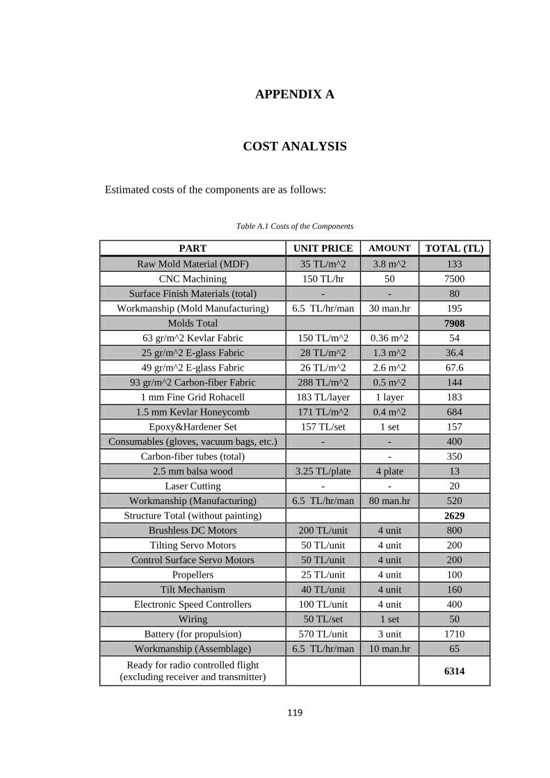
119

APPENDIX A

COST ANALYSIS

Estimated costs of the components are as follows:

Table A.1 Costs of the Components

PART UNIT PRICE AMOUNT TOTAL (TL)

Raw Mold Material (MDF) 35 TL/m^2 3.8 m^2 133

CNC Machining 150 TL/hr 50 7500

Surface Finish Materials (total) - - 80

Workmanship (Mold Manufacturing) 6.5 TL/hr/man 30 man.hr 195

Molds Total

7908

63 gr/m^2 Kevlar Fabric 150 TL/m^2 0.36 m^2 54

25 gr/m^2 E-glass Fabric 28 TL/m^2 1.3 m^2 36.4

49 gr/m^2 E-glass Fabric 26 TL/m^2 2.6 m^2 67.6

93 gr/m^2 Carbon-fiber Fabric 288 TL/m^2 0.5 m^2 144

1 mm Fine Grid Rohacell 183 TL/layer 1 layer 183

1.5 mm Kevlar Honeycomb 171 TL/m^2 0.4 m^2 684

Epoxy&Hardener Set 157 TL/set 1 set 157

Consumables (gloves, vacuum bags, etc.) - - 400

Carbon-fiber tubes (total)

- 350

2.5 mm balsa wood 3.25 TL/plate 4 plate 13

Laser Cutting - - 20

Workmanship (Manufacturing) 6.5 TL/hr/man 80 man.hr 520

Structure Total (without painting)

2629

Brushless DC Motors 200 TL/unit 4 unit 800

Tilting Servo Motors 50 TL/unit 4 unit 200

Control Surface Servo Motors 50 TL/unit 4 unit 200

Propellers 25 TL/unit 4 unit 100

Tilt Mechanism 40 TL/unit 4 unit 160

Electronic Speed Controllers 100 TL/unit 4 unit 400

Wiring 50 TL/set 1 set 50

Battery (for propulsion) 570 TL/unit 3 unit 1710

Workmanship (Assemblage) 6.5 TL/hr/man 10 man.hr 65

Ready for radio controlled flight

(excluding receiver and transmitter) 6314

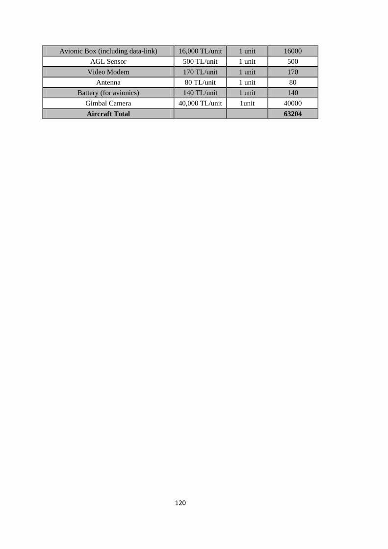
120

Avionic Box (including data-link) 16,000 TL/unit 1 unit 16000

AGL Sensor 500 TL/unit 1 unit 500

Video Modem 170 TL/unit 1 unit 170

Antenna 80 TL/unit 1 unit 80

Battery (for avionics) 140 TL/unit 1 unit 140

Gimbal Camera 40,000 TL/unit 1unit 40000

Aircraft Total

63204

121

APPENDIX B

MOTOR DATASHEET

From [42],

Table B.1Performance of the Motor with Different Propellers

Prop Manf

Prop Size

Input Voltage

Motor Amps

Watts Input

Prop RPM

Pitch Speed

Thrust (Grams)

Thrust (Ounces)

Thrust Eff. (Gr/W)

APC 8x6-E 11.1 12 133.2 9,070 51.5 693.5 24.46 5.21

APC 8x6-SF 11.1 16.56 183.9 8,759 49.8 806 28.43 4.38

APC 8x8-E 11.1 16.48 182.9 8,725 66.1 662.7 23.38 3.62

APC 9x4.5-E 11.1 11.37 126.2 9,127 38.9 821.7 28.98 6.51

APC 9x4.7-SF 11.1 12.48 138.5 9,063 40.3 892.1 31.47 6.44

APC 9x6-E 11.1 13.72 152.3 8,923 50.7 843.3 29.75 5.54

APC 9x6-SF 11.1 24.21 268.8 8,128 46.2 1125.7 39.71 4.19

APC 9x7.5-E 11.1 20.21 224.3 8,426 59.8 918 32.38 4.09

APC 9x7.5 -SF 11.1 27.41 304.2 7,870 55.9 1081.7 38.16 3.56

APC 9x9-E 11.1 23.95 265.9 8,137 69.3 899.7 31.74 3.38

APC 10x3.8 -SF 11.1 21.39 237.4 8,387 30.2 1344.6 47.43 5.66

APC 10x4.7 -SF 11.1 22.51 249.8 8,284 36.9 1361 48.01 5.45

APC 10x5-E 11.1 16.12 178.9 8,769 41.5 1079.7 38.08 6.03

APC 10x6-E 11.1 18.37 203.9 8,593 48.8 1153.2 40.68 5.66

APC 10x7-E 11.1 21.49 238.5 8,349 55.3 1170.1 41.27 4.91

APC 10x7-SF 11.1 31.47 349.3 7,552 50.1 1451.1 51.19 4.15

APC 10x10-E 11.1 30.7 340.8 7,596 71.9 1006.1 35.49 2.95

APC 11x3.8 -SF 11.1 23.9 265.2 8,162 29.4 1522 53.69 5.74

APC 11x4.7-SF 11.1 27.85 309.1 7,832 34.9 1661.9 58.62 5.38

APC 11x7-E 11.1 26.64 295.7 7,951 52.7 1518.6 53.57 5.14

APC 11x8-E 11.1 28.41 315.4 7,790 59 1482.5 52.29 4.7

APC 11x8.5-E 11.1 30.49 338.4 7,613 61.3 1467 51.75 4.34

APC 12x6-E 11.1 28.8 319.7 8,593 48.8 1153.2 40.68 3.61

APC 12x8-E 11.1 34.84 386.7 7,219 54.7 1507.3 53.17 3.9

APC 13x4-E 11.1 25.74 285.7 8,019 30.4 1783.2 62.9 6.24

GEM 9x4.7-C 11.1 12.65 140.4 8,660 38.5 883.6 31.17 6.29

GEM 10x4.5-C 11.1 19 210.9 8,176 34.8 1221.7 43.09 5.79

GEM 11x4.7-C 11.1 25.15 279.2 7,700 34.3 1579.2 55.7 5.66

122

GEM 12x4.5-C 11.1 29.4 326.3 7,372 31.4 1648.1 58.13 5.05

GWS 9x5-DD 11.1 10.99 122 9,185 43.5 824.2 29.07 6.76

GWS 9x5x3-DD 11.1 14.19 157.5 8,879 42 938.5 33.1 5.96

GWS 10x6-DD 11.1 15.41 171 8,842 50.2 1060.6 37.41 6.2

GWS 10x6x3-DD 11.1 19.94 221.3 8,388 47.7 1281.3 45.2 5.79

GWS 11x7-DD 11.1 23.67 262.8 8,184 54.3 1486.4 52.43 5.66

GWS 12x8-DD 11.1 33.5 371.8 7,358 55.7 1763 62.19 4.74

MAS 8x6x3 11.1 12.23 135.8 9,089 51.6 716.7 25.28 5.28

MAS 9x7x3 11.1 19.41 215.4 8,523 56.5 1096.2 38.67 5.09

MAS 10x5x3 11.1 17.21 191 8,699 41.2 1145 40.39 5.99

MAS 10x7x3 11.1 24.52 272.2 8,110 53.8 1416 49.95 5.2

MAS 11x7x3 11.1 28.87 320.5 7,748 51.4 1628.7 57.45 5.08

MAS 11x8x3 11.1 31.08 345 7,556 57.2 1663 58.66 4.82

123

APPENDIX C

JUSTIFICATION OF AERODYNAMICAL OUTPUTS BY CFD

CALCULATIONS

As explained in methodology chapter, no CFD data is used in mathematical model

considering the computational costs. Therefore, after the design phase, CFD

calculations are performed in order to check the validity of the analytical

calculations. Of course, CFD calculations have certain errors and they are not

completely correct; but it is a good practice to compare the order of magnitudes of

the numbers of both sources.

Analysis Conditions

The same physical conditions with the mathematical model are used in analysis. The

temperature, density and the viscosity of the air are assumed to be constant. The

effects of the propellers are not considered in the analysis, it is sure that the prop-

wash changes the forces on the motor booms, especially at low velocities.

- Operating pressure: 88792 Pa

- Air viscosity: 1.7547 x 10-5

Pa.s

- Air temperature: 281.01 K

- Air density: 1.101 kg/m3

Mesh and Boundary Conditions

A rectangular prism shaped domain is used for calculations. The dimensions of the

domain are about 20 times of the aircraft’s maximum lengths at corresponding

directions.

124

Figure C.0.1Boundary Mesh on the Wall Surfaces

Figure C.0.2 Computational Domain

The number of the elements is limited to be about 4.5 million due to the

computational source. A curvature based size function is used in meshing, which is

typical for CFD meshing. 15 boundary layers around the wall surfaces are applied.

125

Figure C.0.3 Cross-section of the motor boom in computational mesh

There is one outlet at the back and the other faces of the domain are inlets. The

velocity is specified at these inlets and it is 20 m/s. The faces of the aircraft are

defined as wall.

Spalart-Almaras turbulence model is used.

α Runs:

Steady state analyses are performed by varying the angle of attack of the aircraft. -

10, -5, 0, 5, 10, 13, 14, 15, 16 and 17 degrees of angles of attack cases are analysed.

Figure C.0.4Lift Coefficient Variation of the Full Aircraft with Angle of Attack

-0.5

0

0.5

1

1.5

2

-15 -10 -5 0 5 10 15 20

CL

α (degrees)

CL vs. α

126

Estimated design lift coefficient at zero angle of attack is 0.655. (see Table 3.3) From

the CFD data CL@α=0ᵒ is found to be 0.613. At cruise velocity with zero angle of

attack, the lift is about 4700 gf.

One of the most important characteristic of an aircraft is . A typical linear curve

of CL vs. α curve is obtained. After a point, flow separation starts and lift is reduced.

At the linear region the slope, which is equal to , is found to be 4.83 rad

-1. It is

very close to the value calculated analytically. (see Table 3.3)

For the full aircraft, the lift begins to drop after 16° of angle of attack. Considering

the incidence angle of the wing, it seems very late. The reason for this situation

seems to be that the lift of the fuselage and tail is remarkable at high angle of attack

values. At 16 degrees of angle of attack, the wing produces 116.1 N of lift. The

fuselage and tail contribution is about 16 N in total. So the, maximum lift coefficient

of the whole aircraft is calculated to be 1.7 (see Figure C.0.4), while the wing’s

maximum lift coefficient is calculated to be 1.55, which is a reasonable value

considering the Cl,max of the wing airfoil.

Another output to be checked is zero lift angle of attack of the airfoil, which is used

for the first estimate of the wing incidence angle. The zero lift angle of attack of the

wing is found to be -3.91° from CFD data. Comparing with the airfoil data, it is a

very good value.

Figure C.0.5 Drag Coefficient Variation of the Full Aircraft with Angle of Attack

0

0.05

0.1

0.15

0.2

0.25

0.3

-15 -10 -5 0 5 10 15 20

CD

α (degrees)

CD vs. α

127

Another critical parameter is the drag coefficient of the aircraft, as the horizontal

flight endurances directly depend on it. At zero angle of attack, CD is found to be

0.062 from CFD calculations. Comparing with the value calculated by analytical

methods (see Table 3.3), the drag estimation used in the model seems reasonable. Of

course, this is a critical issue and more detailed CFD runs or wind tunnel tests are

required to extract stability and control derivatives.

As it can be seen in Figure C.0.5, at the nose of the aircraft, flow stagnates and

creates a high pressure area here, which contributes the total drag significantly. The

payload is modelled as a rounded cylinder for simplicity, but the real geometry of the

payload might create a different flow field. A model with higher fidelity may

enhance the solution.

Figure C.0.6Static Pressure Contours at 20 m/s and Zero Angle of Attack

In detail, the separate values of the components’ drag forces are obtained from CFD

data at zero angle of attack. For motor booms, the values are very close. As the flow

separates behind the boom, it was thought be difficult to estimate the drag force on

the motor booms. There are two possible reasons for the accuracy. Firstly, the

reference value for analytical calculation, which is taken from [45], is an empirical

value; so the estimation is good. Secondly, the CFD calculation is accurate enough.

128

Also for fuselage, which has a cylindrical-like shape, the values are close. CD,0 is not

calculated for tail by using CFD data, because the drag on the tail boom is included

in it. For the wing, the analytically calculated drag force is a bit lower than the CFD

result. The parasite drag coefficient is not calculated for the wing also; because the

proportion of the induced drag and parasite drag cannot be distinguished from the

CFD data.

Table C.1 Drag Force Comparison of CFD Results with Analytical Calculations

DRAG (CFD) (N) DRAG (ANALYTICAL) (N) CD,0 (CFD) CD,0 (Table 3.3)

MOTOR BOOMS 1.834 1.887 0.024507 0.0252

FUSELAGE 0.4226 0.4035 0.005645 0.00539

TAIL 0.285 0.108 (without tail boom)

- 0.00145

WING 2.131 1.769 - 0.00541

In mathematical model, CM,α value is calculated analytically, and the static margin

calculation is made accordingly. In addition to that, CM,α is the basic parameter to

check the longitudinal stability of the aircraft. It can be considered as the damping

of the change in angle of attack, so it must be negative to have a balancing effect

[56]. As it is seen, it is monotonically decreasing with the angle of attack. The value

calculated analytically is -0.38, while the slope of the graph in Figure C.0.7 between

α=0° and α=5° is around -0.37.

129

Figure C.0.7 Body-y Moment Coefficient Variation of the Full Aircraft with Angle of Attack (In Stability Axes

[56])

β Runs:

Steady state analyses are conducted at side-slip angle of 5° and 10° to check the

lateral static stability.

Figure C.0.8Body-z Moment Coefficient Variation of the Full Aircraft with Angle of Attack (In Stability Axes

[56])

-0.4

-0.3

-0.2

-0.1

0

0.1

0.2

0.3

-15 -10 -5 0 5 10 15 20CM

α (degrees)

CM vs. α

0

0.002

0.004

0.006

0.008

0.01

0.012

0.014

0.016

0 2 4 6 8 10 12

CN

β (degrees)

CN vs. β

130

Positive yaw stiffness is required to obtain weathercock stability [56]. As seen in

Figure C.0.8, the moment coefficient in stability-z axis, CN, is increasing with angle

of attack. Thus, CN,β is positive. Numerically, it is around 0.079.

Figure C.0.9 Static Pressure Contours at 20 m/s and 10° Side-slip Angle

131

APPENDIX D

CONCEPTUAL PROBLEM: DRAG FORCE ON MOTOR

BOOMS

Although the airframe concept of this study brings about many advantages, the most

important handicap of the concept seems to be the high drag force on the motor

booms in horizontal flight.

Due to the cylindrical shape of the booms, boundary layer separation behind the

motor booms is seen very clearly. Considering the manufacturing ease, the booms

have no special shape and during the production of the first prototype, they are left as

they are. Some ideas have been generated during this study, but optimizing the shape

of the motor booms is beyond the scope of this study.

In terms of stating the case clearly, it is good practice to examine the CFD data,

which is in a good match with analytical calculations.

Table D.1 Drag Forces on Components at 20 m/s with zero angle of attack

DRAG FORCE (N)

WING 2.131

MOTOR BOOMS (TOTAL) 1.834

FUSELAGE 0.4226

Looking at the Table D.1, it is very clear that the drag on the booms is very close to

the wing’s and four times of the fuselage’s. Considering its surface area, an

extraordinary contribution comes from the booms. This situation is already obvious

from the parasite drag coefficients.

132

As it can be seen in Figure D.0.1, flow separates after a point near to the top points

of the cylinder, leaving a low pressure zone behind the boom (see Figure D.0.2) . It

creates a high drag force on the boom.

Figure D.0.1Velocity Vectors around the Motor Boom at 20 m/s with zero angle of attack

Figure D.0.2 Static Pressure Contours around the Motor Boom at 20 m/s with zero angle of attack

This situation drastically decreases the horizontal flight endurance of the aircraft.

Almost 40 % of the total drag is due to the motor booms. If the booms are removed,

the drag force reduces to 3.05 N according to the CFD data. (see Figure D.0.3) It can

be also said that the motor booms decreases the horizontal flight endurance by almost

133

40 %. This cost is too much for sake of vertical flight capabilities; and also it is

avoidable.

Figure D.0.3 Static Pressure Contours of the Aircraft Version without Motor Booms at 20 m/s with zero angle of

attack

This is a very common problem in various disciplines of engineering. So, there are a

lot of studies related with it. For this concept, there are two main approaches to solve

the drag problem.

The first approach is to have streamline-shaped motor boom. A streamline-shaped

boom prevents the flow separation and the form drag would decrease. [56]

Figure D.0.4Separation Points on several 2-d elliptical and Jukowsky shapes determined by theoretical analysis

of the boundary layer flow (from [45])

It is simply placing fairings on motor booms. Coating the carbon fiber booms with a

non-structural material is a solution. The diameter of the boom still must be large

enough to have required strength, as it carries 1.5 kgf at its tip during the hovering.

134

On the other hand, if the thickness ratio is small, the length of the fairing becomes

larger. Two disadvantages come with that. The first one is that in hovering

downwash of the propeller is faced directly by the fairing. (see Figure 1.4) Out of the

ground effect, this situation decreases the carrying capacity as explained before. On

the other hand, this problem may be solved by tilting the fairing synchronously with

the propellers like a tilt-wing aircraft. The second disadvantage is the possibility to

distort the upstream of the wing. Eliminating and even turning it to an advantage is

possible by an integrated servo controller, which tilts the fairing; but this would be a

very complicated system. Besides, stability problems may arise due to these fairings.

Equivalently strong booms may be replaced. The diameter of the boom may be

reduced or an elliptical boom may be used but the prices of the elliptical booms are

very high and the production of them is rather hard.

Figure D.0.5 A Possible Tilting-Fairing Solution to Reduce the Form Drag (Upper configuration in horizontal

flight and lower configuration in hovering)

135

The second approach is to obtain a thicker boundary layer and postpone the

separation like in well-known golf ball example.

Figure D.0.6 Delay Separation on Golf Ball (from [57])

Figure D.0.7The Mechanism of Flow Separation Delaying by Dimples on Surface (from [58])

Briefly, the flow separation occurs when the momentum of the flow is not enough to

overcome the pressure gradient. Separation bubbles are generated in the dimples and

this situation induces a turbulent boundary layer. The momentum of the turbulent

boundary layer is higher than laminar. So the flow can reattach to the wall and the

separation is delayed [58].

This phenomenon is dependent to Reynolds number. For a smooth circular cylinder,

there is a critical Reynolds number that the drag coefficient dramatically changes.

That point corresponds to the separation. It is between Reynolds number of 1e+5 and

1e+6 for a smooth sphere. In this studies’ specific case, the flow on the motor booms

would have a Reynolds number around 20000, in case there is no prop-wash on

136

them. On the other hand, considering that they are at a point that is very close to the

propellers; it can be expected to have a close Re value to 1e+5 on the booms. Thus, it

seems suitable to apply this methodology for reducing the drag. Besides, it should be

taken into account that the prop-wash is a complex flow with high vortices, so the

case may have different characteristics with golf ball or other simple cases.

Figure D.0.8 Drag Coefficient Variation of Some Geometries with Reynolds Number ([from[58])

Another study with similar logic but different practice is about manipulating the

upstream flow. [59] Again, the same range of Reynolds numbers is investigated. A

turbulator rod is set in front of the cylinder to increase the turbulence in upstream of

the cylinder. In optimum conditions, it is said that a drag reduction of 63 % could

obtained outcome of this study.

Figure D.0.9 Sketch of the Experimental Flow Geometry [59] (from [59])

137

Figure D.0.10Flow Visualization of the Experiment in [59] (from [59])

This is a similar method used by radio control (R/C) modellers with same purpose.

For the specific case of this aircraft, placing the manipulating rod in front of the

boom can be hard due to physical limitations, but it would be a conceptually

straightforward and cheap option.

On the other hand, aft of the boom is more available in terms of physical space.

Placing a “splitter plate” would be an option to reduce the drag [45]. Theoretical

background can be explained briefly as such: The motion characteristic of the vortex

138

street behind the circular cylinder is affected by placing a splitter plane at the

centreline of it. Behind the cylinder, Strouhal number is decreased and the local

pressure increase. [45], [60]. Thus, a higher pressure field is obtained behind the

cylinder and the total form drag reduces, as the pressure difference between both

sides is decreased.

Figure D.0.11 Influence of Splitter Plates on Drag Coefficients of Several Geometries (from [45])

139

Figure D.0.12Effects of Splitter Plates upon Stv and Localised Pressure Coefficient (from [61])

This method is good for being easy and cheap to manufacture; but the problem of

decreasing carrying capacity in hovering may arise due to the downwash hitting the

splitter plate. A careful splitter plate design with trade-off analyses should be made

in case of using this method.

141

APPENDIX E

JUSTIFICATION OF THE STRUCTURAL DESIGN OF THE

AIRCRAFT BY STATIC LOADING

The structural design of the aircraft is tested by static wing loading of 1g and 3g; and

motor boom tip loading of 1.5 kgf. In wing loading tests, elliptical load distribution is

assumed. The loads are calculated along the span by integrating the load per unit

length, q [N/m]. A Riemann sum approach is used to calculate the loads at the

stations. In below formula, “W” refers the total load on one wing in Newton, and “b”

refers the wing span. (

√

Considering the mission concept of the aircraft, the maximum loading in a possible

flight envelope is thought to be around 2g from past experiences. By applying a

factor of safety of 1.5, 3g static wing loading test is realized.

Figure E.0.1 1g Static Wing Loading Test (about 2.5kg at each wing)

142

Figure E. 0.2 1g Static Wing Loading Test (about 2.5kg at each wing)

Table E.1 Loads at the Stations in 1g Static Wing Loading Test

Station #

Station position (from root)(m) Load (kg)

x1 0.8 0.15

x2 0.6 0.35

x3 0.48 0.45

x4 0.35 0.5

x5 0.2 0.53

x6 0.1 0.55

SUM 2.498

0

0.1

0.2

0.3

0.4

0.5

0.6

0 0.2 0.4 0.6 0.8 1

Load

(N

)

Position on Half Wing Span (m)

Load Distribution on Half Wing Span

143

In 1g test, a total load of 5 kg (2.5 kg at each wing) is applied from the quarter chord

of the wing. About 3.5 mm of wing tip deflection is measured and no sign of fracture

or surface buckling is observed.

Figure E. 0.3 Wing Deformation in 1g Static Wing Loading Test

In 3g test, a total load of 15 kg (7.5 kg at each wing) is applied from the quarter

chord of the wing. About 21.5 mm of wing tip deflection is measured and no sign of

fracture or surface buckling is observed.

Table E.2 Loads at the Stations in 3g Static Wing Loading Test

Station #

Station position (from root)(m) Load (kg)

x1 0.8 0.50

x2 0.6 1.17

x3 0.45 1.38

x4 0.35 1.45

x5 0.2 1.49

x6 0.1 1.51

SUM 7.5

0.35

0.55

0.75

0.95

1.15

1.35

1.55

0 0.2 0.4 0.6 0.8 1

Load

(N

)

Position on Half Wing Span (m)

Load Distribution on Half Wing Span

144

Figure E.0.4 3g Static Wing Loading Test (about 7.5 kg at each wing)

Figure E.0.5 Wing Deformation in 1g Static Wing Loading Test

For the motor booms, 1.5 kgf, which is the maximum thrust value of the propellers,

is applied at their tips. In average 1.5 mm of tip deflection is measured and no sign of

fracture is observed.

145

Figure E.0.6Static Loading of Motor Booms

DESIGN AND MANUFACTURING OF A QUAD TILT …etd.lib.metu.edu.tr/upload/12618110/index.pdf · ·...

Documents

Transcript of DESIGN AND MANUFACTURING OF A QUAD TILT …etd.lib.metu.edu.tr/upload/12618110/index.pdf · ·...