University of Central Florida University of Central Florida

STARS STARS

Electronic Theses and Dissertations, 2004-2019

2005

Design And Implementation Of Wireles Sensor Networks For Design And Implementation Of Wireles Sensor Networks For

Parking Management System Parking Management System

Sudhir Chandrasekar Kora University of Central Florida

Part of the Electrical and Electronics Commons

Find similar works at: https://stars.library.ucf.edu/etd

University of Central Florida Libraries http://library.ucf.edu

This Masters Thesis (Open Access) is brought to you for free and open access by STARS. It has been accepted for

inclusion in Electronic Theses and Dissertations, 2004-2019 by an authorized administrator of STARS. For more

information, please contact STARS@ucf.edu.

STARS Citation STARS Citation Kora, Sudhir Chandrasekar, "Design And Implementation Of Wireles Sensor Networks For Parking Management System" (2005). Electronic Theses and Dissertations, 2004-2019. 458. https://stars.library.ucf.edu/etd/458

DESIGN AND IMPLEMENTATION

OF

WIRELESS SENSOR NETWORKS

FOR PARKING MANAGEMENT SYSTEM

by

SUDHIR CHANRASEKAR KORA B.S. University of Madras, 2001

A thesis submitted in partial fulfillment of the requirements for the degree of Master of Science

in the Department of Electrical and Computer Engineering in the College of Engineering and Computer Science

at the University of Central Florida Orlando, Florida

Summer Term

2005

© 2005 Sudhir Kora

ii

ABSTRACT

The technology of wirelessly networked micro sensors promises to revolutionize the way we

interact with the physical environment. A new approach to solve parking-related issues of

vehicles in parking lots using wireless sensor networks is presented. This approach enables the

implementation of the Parking Management System (PMS®) in public parking lots found in

Airports, Commercial Buildings, Universities, etc. The design architecture of the sensor nodes is

discussed here. An overall view of the sensor network, which covers the whole of the parking

lot, is also summarized. Detailed description of the software architecture that supports the

hardware is provided. A sample experiment for detecting the movement of vehicles by placing

the sensor nodes allowing vehicles to pass over it is performed. The readings are sent to a local

database server, which gives an indication of the actual number of vehicles parked in the

building at any time. This application-oriented project also identifies important areas of further

work in power management, communication, collaborative signal processing and parking

management.

iii

ACKNOWLEDGMENTS

This thesis work would not have been possible without the motivation and support of a

number of people who deserve special mention here. My foremost gratitude goes to my chair,

Dr. Ronald Phillips, who provided me guidance for the development of this work.

I would also like to thank my advisor and co-chair Dr. Chan Ham, whose constant

encouragement has been the motivating factor for my work here. I feel very fortunate for having

an advisor like Dr. Chan Ham, who understood the difficulty, that I faced in my research and

showed constant support throughout my thesis work. I remain thankful to him for his advice and

help on all matters professional and personal.

My special thanks also goes to Dr. Stephen Watson for being on my thesis committee and for

offering suggestions on writing the thesis draft.

Finally, I would like to thank my parents, sister and brother-in-law who have always shown

their love, support and blessings, which had been a constant encouragement throughout my stay

here at UCF. I also would like to thank Anil, Sriram, Suruchi and all of my friends at UCF for

their help and support.

iv

TABLE OF CONTENTS

LIST OF FIGURES ..................................................................................................................... viii

CHAPTER ONE: INTRODUCTION............................................................................................. 1

1.1 Technical Background .......................................................................................................... 1

1.2 Sensor Network Applications ............................................................................................... 2

1.3 Motivation............................................................................................................................. 4

1.4 Challenges affecting the design ............................................................................................ 5

1.5 Chapter Organization ............................................................................................................ 5

CHAPTER TWO: HARDWARE AND SOFTWARE ARCHITECTURE OF SENSOR NODES

......................................................................................................................................................... 6

2.1 Overview............................................................................................................................... 6

2.2 Generalized architecture of a wireless sensor node .............................................................. 6

2.2.1 Computing Subsystem ............................................................................................... 7

2.2.2 Communication Subsystem ....................................................................................... 7

2.2.3 Sensing Subsystem .................................................................................................... 8

2.2.4 Power Subsystem....................................................................................................... 8

2.3 Sensor Node Architecture ..................................................................................................... 8

2.4 Sensor Board....................................................................................................................... 10

2.5 MIB510 Interface Board ..................................................................................................... 11

2.6 Magnetometer ..................................................................................................................... 12

v

2.6.1 Basic Device Operation ........................................................................................... 12

2.6.2 Vehicle Detection .................................................................................................... 14

2.6.3 SET/RESET and OFFSET straps ............................................................................ 15

2.7 Software Architecture for Wireless Sensor Networks ........................................................ 15

2.7.1 TinyOS Component Model...................................................................................... 16

2.8 NesC Language................................................................................................................... 17

2.8.1 Example Application ............................................................................................... 17

CHAPTER THREE: PARKING MANAGEMENT SYSTEM DESIGN .................................... 19

3.1 Introduction......................................................................................................................... 19

3.2 System Requirements.......................................................................................................... 20

3.2.1 Hierarchical network................................................................................................ 20

3.2.2 Extended Life of Sensor Networks.......................................................................... 20

3.2.3 System Stability ....................................................................................................... 20

3.2.4 Additional Sensing Capabilities............................................................................... 21

3.3 Sensor Network Architecture.............................................................................................. 21

3.3.1 Low Tier Architecture ............................................................................................. 23

3.3.2 Middle Tier Architecture ......................................................................................... 24

3.3.3 Higher Tier Architecture.......................................................................................... 24

CHAPTER 4: EXPERIMENTAL READINGS AND SIMULATION........................................ 26

4.1 NesC Implementation ......................................................................................................... 26

4.1.1 The Magnetometer.nc Configuration....................................................................... 27

4.1.2 The MagnetometerM.nc Module ............................................................................. 28

4.2 Message Format .................................................................................................................. 31

4.3 Data Conversion.................................................................................................................. 31

vi

4.4 Experiments and Data Analysis .......................................................................................... 32

4.5 Simulation of the Parking Management System................................................................. 35

4.5.1 Algorithm Design .................................................................................................... 36

CHAPTER FIVE: CONCLUSION............................................................................................... 39

APPENDIX A............................................................................................................................... 40

APPENDIX B ............................................................................................................................... 44

LIST OF REFERENCES.............................................................................................................. 47

vii

LIST OF FIGURES

Figure 2.1 System architecture of a wireless sensor mode ............................................................. 7

Figure 2.2 Block Diagram of Mica2 Sensor Node ......................................................................... 9

Figure 2.3 MICA2 Sensor Node ................................................................................................... 10

Figure 2.4 MTS310CA Sensor Board........................................................................................... 11

Figure 2.5 MIB510 Interface Board.............................................................................................. 12

Figure 2.6 Wheatstone bridge circuit............................................................................................ 13

Figure 2.7 Magnetoresistive Effect............................................................................................... 14

Figure 2.8 Perturbations in earth’s magnetic field caused by a moving vehicle .......................... 15

Figure 3.1 Simplified layout showing sensor placement in a parking lot..................................... 22

Figure 3.2 System Architecture of Parking Management System using Wireless Sensor Networks

............................................................................................................................................... 23

Figure 4.1 Block Diagram of Experimental Setup........................................................................ 33

Figure 4.2 Detection of a single moving car................................................................................. 34

Figure 4.3 Detection of two moving cars in a bumper-to-bumper fashion................................... 35

Figure 4.4 Algorithm for simulation of PMS................................................................................ 37

Figure 4.5 Snapshots of parking lot simulation file...................................................................... 38

viii

CHAPTER ONE: INTRODUCTION

With advances in micro-electrical-mechanical systems (MEMS) technology, wireless

communications, and digital electronics, multifunctional sensor nodes have emerged which are

primarily low cost, consume less power, small in size and communicate over short distances.

This phenomenal growth is in accordance to “Moore’s law”, which states that the number of

transistors per square inch on integrated circuits has doubled every year since the integrated

circuit was invented. In recent years, wireless communication has grown at a tremendous pace

resulting in an exponential growth. Wireless sensor networks has contributed to this rapid growth

due to the increasing exchange of data in internet services such as World Wide Web, e-mail and

data file transfers.

1.1 Technical Background

Remote sensing and measuring is an important field of engineering that has unlimited

growth and potential. The Mars Exploration Rovers launched in mid 2003 in an attempt to find

the history of water on Mars is a suitable example to state the above fact. This field of

technology has come a long way from meter reading to data acquisition systems to a new era of

wireless sensor networks (WSN). These sensor networks provide an intelligent platform to

gather, analyze and react on data without human intervention. A wireless sensor network can be

defined as an intelligent system capable of performing distributed sensing and processing, along

with collaborative processing and decision making for carrying out a particular task.

Self-configuring wireless sensor networks can be invaluable in many civil and military

applications for collecting, processing, and disseminating wide ranges of complex environmental

data [1]. The WINS [2] and SmartDust [3] projects integrate sensing, computing and wireless

1

communication capabilities into a small form factor. Wireless distributed sensor networks

require application driven system design and can be deployed for specific tasks and applications.

In the next several years’ sensor networks are destined to grow into a phenomenal rate touching

everyone’s life in some way or the other.

A lot of our daily operations require information gathering from remote locations. One of

the merits of building a wireless sensor network for information gathering is the flexibility it

allows in adding sensors and changing the layout of the system. Wireless sensor networks consist

of a large number of densely deployed sensor nodes. These nodes incorporate wireless

transceivers so that communication and networking are enabled. Additionally, self-organizing

capability of the sensor network enables them to have very little network setup. In an ideal case,

individual nodes are battery powered with a long lifetime and cost very little. Wireless sensor

networks are similar to Ad-hoc networks in many ways. These sensor networks utilize the self-

organizing and routing technologies developed by the ad-hoc research community. These

systems are often limited by a number of factors, which include energy usage, latency,

throughput, scalability, adaptability, and lifetime requirements [1]. Innovative design techniques

are required to overcome the challenges of limited energy and communication bandwidth

resources. The parameters of the sensor network application have to be thoroughly understood to

design good protocols that improve the efficiency and longevity of the network.

1.2 Sensor Network Applications

Networked microsensors technology is a key technology for the 21st century. Cheap,

smart devices with multiple on-board sensors, networked by means of wireless links and the

Internet provide unprecedented opportunities for instrumenting, and controlling the

environment. One of the key features of sensor networks is that any large sensing task can be

2

broken down into small tasks, which can be distributed, to a group of sensors that coordinate

among themselves. The application fields of wireless sensor networks are only bound by our

imagination. Some of the important applications where a lot of research is focused include

Infrastructure security, Environment and habitat monitoring, Traffic control, Home networking

and building automation, Emergency Operations (forest fire detection), Elderly home care,

Industrial Monitoring etc [1].

Infrastructure security includes structural health monitoring of bridges, dams, buildings

and other physical structures, to analyze the local response of the civil structure. Environmental

sensors are used to study vegetation response to climatic trends and diseases. Acoustic and

imaging sensors can be used to identify, track, and measure the population of endangered

species. Cheap sensors with embedded networking capability can be deployed at every road

intersection to detect and count vehicle traffic and estimate its speed. Deployment of wireless

sensors throughout a building enables, continuous monitoring of weather conditions such as

temperature, humidity and also occupancy. Controlling of window and door locks, appliance

operation, energy management, or remote monitoring of environmental conditions are some of

the tasks that can be achieved using wireless sensor networks within the home. Sensor networks

can also help firefighters in understanding the direction of the spread of fire, thermal gradients,

wind, humidity, and other parameters and responding more quickly and effectively to prevent

the spread of fire. Research is going on at Intel and other labs around the country to develop

ways using wireless sensors to help the elderly, and others who need assistance with everyday

activities. Distributed sensors and controls can enable fundamental advances in manufacturing

and condition-based maintenance. Wireless Sensor Networks are low cost mobile systems that

can cover the entire enterprise.

3

1.3 Motivation

A majority of research work has been targeted to use sensor networks for habitat

monitoring and surveillance, where the main factor is to sense environmental factors such as

light, temperature etc [4]. In several of these applications, data is generated only when an

interesting event occurs or when prompted by user. One application, which requires periodic and

continuous monitoring, is monitoring vehicle movement in and out of a parking garage.

Deploying sensor nodes in parking garages can enable long-term data collection at a very high

scale of resolution. The wireless sensor domain nodes can provide localized measurements and

information more easily than provided by traditional instrumentation. In short, networking of a

large number of sensor nodes enables high quality sensing networks with the advantages of easy

deployment and fault-tolerance. The wireless networking of micro sensors is comparatively

cheaper than wired-networking. Also a sensor network comprises of large number of sensor

nodes densely deployed closer to the phenomenon of interest. In the existing wired security

systems, all sensor nodes need to be connected by wires, whenever they are setup. It becomes

expensive to maintain and mend, if cables connect the sensor nodes. It is also hard to change the

position of a sensor node, and if a portion of the wired network is destroyed by an accident,

sensor nodes corresponding to that portion are divested of their function. This case is totally

eliminated in the case of short-range wireless communication technology.

The primary goal of this thesis work is to develop a solution for parking problem, faced

everyday by the community. Parking garages in most of the locations tend to be full, especially

during the peak hours. Lot of commuters waste precious time in looking for a parking spot and

in the end have to park their vehicle far from the venue of location. Providing suitable

information to the commuter in finding the parking space can eliminate a lot of time wasted in

this process. Although a number of parking monitoring solution exists in European and East

4

Asian Countries, wireless monitoring using sensor networks is rather new as suggested in this

thesis work. With rapid growth in sensor technology, sensors may cost a few cents in the near

future and automating a parking lot using sensor networks may become a reality.

1.4 Challenges affecting the design

One of the prime factors, which affect sensor life in a sensor network, is power. The

sensor nodes are battery powered and additional nodes are needed in a network to replace the

dead ones. Various power saving protocols are designed to suit sensor nodes. The nodes are

made to remain in the sleep mode when they are not active. The sensor nodes need to

communicate with the base station at any point of time and this further increase the complexity

in designing the sensor network. Some other factors, which pose challenge in design of the

sensor network, include transmission rate, synchronization rate, memory constraints etc. These

limitations can be overcome by designing application specific optimized wireless sensor network

design.

1.5 Chapter Organization

The chapters in this thesis are summarized as follows. Chapter 2 provides the details of

the hardware and software architecture of the sensor network. Chapter 3 deals with the system

level architecture of the parking management system. Chapter 4 deals with the experimental

results and simulation of the network architecture. The work finally concludes with a conclusion

report in Chapter 5. The source code and other details are provided in the Appendix section.

5

CHAPTER TWO: HARDWARE AND SOFTWARE ARCHITECTURE OF SENSOR NODES

2.1 Overview

The overall operation of Parking Management System (PMS) can be broken into two

simple steps:

I) Individual nodes gather information from the environment to generate and

later deliver report messages to the base station,

II) The base station aggregates and analyzes the received report messages and

decides the occurrence of unusual event in the area of interest.

In this chapter we focus on the hardware architecture of a wireless sensor node and also the

embedded software architecture. The hardware and software described here play an important

role in the development of the PMS.

2.2 Generalized architecture of a wireless sensor node There are several wireless sensor projects being developed for supporting ubiquitous

computing. WINS [2], MICA [5], EYES [6] are some to name a few. These sensor nodes use

cheap, commercially available components in its design. The system architecture of a wireless

sensor node is shown in the figure 2.1. The node is comprised of four major subsystems, i) a

computing subsystem, ii) a communication subsystem iii) a sensing subsystem iv) a power

supply subsystem.

6

Micro Controller Unit

S E N S O R S

R A D I O

Memory

Power Supply Unit

Figure 2.1 System architecture of a wireless sensor mode

2.2.1 Computing Subsystem

The central core of the whole sensor node, which performs computations for sensing,

acquiring, processing, storing and communicating the data, is the computing subsystem. It

comprises of a microcontroller or multiple processors and memory chips. Micro controllers like

ATMEGA128 or microprocessors like StrongARM 1100, SH-4 etc. are used, based on the

application requirements. In this subsystem, the data path is connected to the rest of the system

components through a shared interconnect [8]. Memory, I/O ports, system timers etc. are

attached to this interconnect. The communication between the core architecture and the

peripherals is through a memory-mapped interface. The interface also allows the individual

peripherals to interact with each other.

2.2.2 Communication Subsystem

This subsystem is responsible for data and message transfer between neighboring nodes.

It consists of a transceiver and a set of discrete components for operation. The transceivers are

short-range low power chips operating on ISM band of radio frequencies. External antenna is

7

used to improve the transmission range. Off all the three subsystems, namely, computing,

communication and sensing, this subsystem consumes the maximum power. Suitable protocols

are designed to enable the transceiver to operate in selected modes like sleep, transmit and

receive to minimize power consumption.

2.2.3 Sensing Subsystem

Advances in Micro-electromechanical Systems (MEMS) have enabled the development

of single-chip sensors that can be used to measure a host of physical parameters. These sensors

are typically transducers that convert the sensed physical quantity into current and voltages.

2.2.4 Power Subsystem

A DC-DC converter regulates the supply voltage of the system by providing a constant

power supply. A pair of AA batteries can be used to provide energy for operation.

2.3 Sensor Node Architecture

We use MICA2 hardware for the development work done in this thesis. MICA2 is built

using a single CPU and uses the TinyOS operating system. The block diagram shows the MICA2

architecture in figure 2.2.

The Microcontroller is an 8-bit ATMega128L running at 7.37 MHz [5, 8]. It has 128

Kbytes of flash program memory and 4 Kbytes of system RAM (SRAM). Additionally, it has an

8 channel, 10-bit ADC and 53 programmable I/O lines. It has an external UART and a SPI port.

The RF Module consists of a Chipcon CC1000 transceiver and a set of discrete

components to operate the radio. The radio operates in the 916 MHz ISM band of frequency

supporting a maximum number of 50 channels. The outdoor range can extend up to 500 ft with

8

data rate of 38.4 Kbits/sec. The typical current draw by the transceiver during transmit, receive

and sleep stages are 25 mA, 8 mA, and less than 1 µA respectively.

51-Pin I/O Expansion Connector Digital I/O 8 Analog I/O 8 Programming Lines

Atmega 128L Micro-controller

Transmission Power Control

Hardware Accelerators

Chipcon CC1000 Radio Transceiver

SPIBus

512 KB Flash Data Logger Memory

Figure 2.2 Block Diagram of Mica2 Sensor Node

Atmel AT45DB014B is a 512KB flash data logger that provides persistent data storage. It

stores sensor data as well as program images that are to be sent over the network and

programmed onto the Microconroller. A SPI Interface connects the data logger to the

Microcontroller.

The power source for the sensor node includes 2 AA type batteries. The typical capacity

is 2000mA-hr. A 3.3 V booster, which is generally included in the MICA configuration, is absent

here. A pictorial representation of the sensor node used for the experiments is shown in figure

2.3.

9

Figure 2.3 MICA2 Sensor Node

The I/O interface consists of a 51-pin expansion connector designed to interface with

sensing and programming boards. The expansion connector is divided into sections of 8 analog

lines, 8 power control lines, 3 PWM lines, two analog compare lines, 4 external interrupt lines,

an I2C bus, an SPI bus, a serial port, and a collection of lines dedicated to programming the

microcontroller. The expansion connector can also be used to program the device.

2.4 Sensor Board

The sensor board used in this thesis work is MTS310CA sensor board shown in Figure

2.4. It has a small form factor with functionality of a wide range of sensing parameters [9]. It has

a microphone, sounder, light sensor, thermistor (Panasonic ERT-J1VR103J), 2-Axis

Accelerometer (ADXL202JE) and a 2-Axis Magnetometer (Honeywell HMC1002). The 2-Axis

magnetometer forms the principal object of this thesis work. This sensor is capable of detecting

vehicles at a radius of 15 feet. In section 2.6, the functioning of the magnetometer is explained in

detail. The sensor board has a 51-pin expansion connector to connect to the sensor node and also

to the interface board.

10

Figure 2.4 MTS310CA Sensor Board

2.5 MIB510 Interface Board

The MIB510 interface board can be used in conjunction with the MICA2 sensor nodes. It

has an external power adapter to optionally supply power to the sensor node and an interface for

RS232 serial port. The RS-232 interface is a standard single channel bi-directional interface with

a DB9 connector to provide interface to an external computer [8]. It uses transmit and receive

lines only. The sensor node is programmed by connecting the MIB510 interface board to the

serial port of the computer, and executing the required programming software. The MIB510 has

an on-board in-system processor (ISP) to program the Motes. The code is downloaded to the ISP

through the RS-232 serial port. The ISP then programs the code into the node. The ISP and the

node share the same serial port. A pictorial representation of the interface board is shown in

figure2.5

11

Figure 2.5 MIB510 Interface Board

2.6 Magnetometer

Magnetometer forms the main component of the data acquisition system in this thesis

work. The system uses as little energy as possible to take an accurate magnetic field strength

measurement. For detecting the movement of vehicle, the sensor output is typically sampled at

100 Hz. The sensor node uses a HMC1002 anisotropic magnetoresistive (AMR) magnetic field

sensor from Honeywell to count the number of passing vehicles. The magnetoresistive sensors

are configured as a 4-element wheatstone bridge. They convert magnetic fields to a differential

output voltage and are capable of sensing magnetic fields as low as 30 µgauss [10,11]. These

MRs offer a small, low cost, high sensitivity and high reliability solution for low field magnetic

sensing. Hence they form a very important element of this work. HMC 1002 contains two

sensors for the x- and y- field measurements.

2.6.1 Basic Device Operation

HMC1002 are simple resistive bridge devices (Figure 1) that only require a supply

voltage to measure magnetic fields. When a voltage from 0 to 10 volts is connected to Vbridge,

12

as shown in figure 2.6, the sensor begins measuring any ambient, or applied, magnetic field in

the sensitive axis. The sensor also has two on-chip magnetically coupled straps-the OFFSET

STRAP and the Set/Reset strap. An AMR sensor is made from a thin film of nickel-iron

(Permalloy) thin film deposited on a silicon wafer and patterned as a resistive strip. The nickel-

iron strip has the property to change its resistance in the presence of a magnetic field leading to a

corresponding change in voltage output.

When an external magnetic field is applied normal to the side of the thin film, it causes

the magnetization vector (M) to rotate and change angle. The resistance value will be forced to

vary by ∆R/R and this change will produce a voltage output change in the Wheatstone bridge.

This change in the Permalloy resistance is termed as the magnetoresistive effect, which is

directly related to the angle of the current flow and the magnetization vector. This is represented

in the figure 2.7 below.

Figure 2.6 Wheatstone bridge circuit

13

Figure 2.7 Magnetoresistive Effect

2.6.2 Vehicle Detection

The Magnetometers available today are capable of sensing magnetic fields below 1

gauss. They can be used for detecting vehicles, which are ferrous objects that disturb the earth’s

field. When a vehicle moves in an arbitrary direction the magnetic field of the earth induces a

field that points through the north south direction through the vehicle. In addition to the earth’s

magnetic field, the vehicle also possesses a permanent magnetic field that tends to rotate with it.

These two fields interact with each other resulting in a total magnetic field. The overall magnetic

field can be modeled as a simple magnetic dipole. Thus the magnetic field of a moving vehicle

can be detected by properly placing an AMR sensor on the side of a roadway. A figure

explaining the perturbations in the earth’s magnetic field induced by magnetic dipoles in a

ferrous metal vehicle is shown below. The distortion of the earth’s magnetic field created as a

vehicle enters and passes through the detection zone of a magnetic sensor is also shown in the

figure 2.8 below.

14

Figure 2.8 Perturbations in earth’s magnetic field caused by a moving vehicle

2.6.3 SET/RESET and OFFSET straps

Strong magnetic fields (more than 10 gauss) could upset or flip the polarity of film

magnetization, thus changing the sensor characteristics. When this happens, a strong restoring

magnetic field must be applied momentarily to restore, or set, the sensor characteristics. This

effect is referred to as applying a set pulse or reset pulse. The OFFSET strap creates an on-axis

magnetic field, which can be used to put the sensor inside a feedback loop. The SET/RESET

strap is used to create a strong cross-axis magnetic field to re-align the domains with the sensor

axis, which restores the sensor’s sensitivity and accuracy.

2.7 Software Architecture for Wireless Sensor Networks

The software for the wireless sensor networks should be such that it should be able to

coordinate and develop the raw hardware capabilities into a complete system. In order to cater to

these requirements, the software, binding the hardware components should be very efficient in

terms of memory, processor and power requirements. In addition to these requirements, the

operating system must support the concurrency intensive operations of the hardware devices. It

means that the data flows of different types must be kept moving simultaneously. The system

15

utilizing the operating system must also provide efficient modularity and robustness. An optimal

solution for this is a tiny micro-threaded OS called TinyOS [5,12]. TinyOS is an operating

system that retains the hardware design characteristics such as small physical size, modest active

power load, while supporting concurrency intensive operation.

2.7.1 TinyOS Component Model

The system specification of TinyOS includes a list of components plus a specification for

the interconnection between the components. A component in TinyOS has four interrelated parts:

a set of command handlers, a set of event handlers, an encapsulated fixed-size frame and a

bundle of simple tasks. The fixed-size frame prevents the overhead associated with dynamic

allocation. The memory requirements of the compilation of a component can be known which

results in saving the execution time. Commands are requests made to lower level components. A

command must provide feedback to its caller about its state of action. Event handlers performs

multiple tasks such as depositing information into its frame, posting tasks, signaling higher level

events or calling lower level commands. They connect lower level components to hardware

interrupts. Tasks perform the primary work of calling lower level commands, signaling higher-

level events and scheduling other tasks within a component. In general, components belong to

one of the three categories: hardware abstractions, synthetic hardware and high-level software

components. The functions of these component types are varied. Hardware abstraction

components connect physical hardware into TinyOS component model. Synthetic hardware

components simulate the behavior of advanced hardware. The high-level software components

perform control, routing and all data transfers. TinyOS offers several key features that make it a

suitable choice for sensor networks. Small physical size, concurrency intensive operation,

16

efficient modularity, limited physical parallelism and robustness are the main characteristics of

TinyOS.

2.8 NesC Language

NesC is a new language developed primarily for the embedded systems. The syntax of

NesC is similar to that of C but it supports concurrency models as done by the operating system

TinyOS [13]. In addition to this, NesC also provides mechanisms for structuring, naming and

linking software components into robust network embedded systems. These unique features of

NesC allow programmers to develop applications of wireless sensor networks by individually

coding modules and components and linking them together to form a complete application. The

application developed in this thesis work is programmed using NesC. A simple application called

Blink is described in the next section that gives a better understanding of the programming

structure of NesC.

2.8.1 Example Application

An application in TinyOS can be simply broken down into components, which can be of

two types: module or configuration. In this particular application named Blink, the LED’s on the

programming node are made to blink in an orderly fashion. A sample code of the module and

component are shown here for better understanding. In General case, the module and the

configurations are named after the application itself to avoid confusion. The Blink module is as

follows

module BlinkM{ provides { interface StdControl; } uses { interface Timer;

17

interface Leds; } } In the first line, BlinkM implements the StdControl interface. The BlinkM module also uses two

interfaces: Leds and Timer. This means that BlinkM may call any command declared in the

interfaces it uses and must also implement any events declared in those interfaces. The

configuration for the Blink application is dealt below:

configuration Blink { } implementation { components Main, BlinkM, SingleTimer, LedsC; Main.StdControl -> BlinkM.StdControl; Main.StdControl -> SingleTimer.StdControl; BlinkM.Timer -> SingleTimer.Timer; BlinkM.Leds -> LedsC; } The keyword configuration indicated that this is a configuration file. The line following the

keyword implementation indicates the set of components referenced here. In this case Main,

BlinkM, SingleTimer and LedsC are the components used. In all TinyOS applications Main is

the first component that is executed first. The –> is used for connecting interfaces used by

components to interfaces used by others. From the above code, it is clear that the main

application is linked to the Blink module, which is connected to the timer and LED’s

components. In this manner tiny components are wired together to develop an entire application.

The application developed in this thesis work is also wired in a similar fashion, which is shown

in chapter 4.

18

CHAPTER THREE: PARKING MANAGEMENT SYSTEM DESIGN

3.1 Introduction

Parking Management System (PMS) is a real-time application and requires continuous

monitoring and tracking of vehicles inside the parking lot. The information gathered by the

sensors need to be periodically updated, to give accurate on the spot report of available parking

spaces in the lot, at all times. It is important to note that during peak hours, cars flood parking

lots at an extremely rapid rate. Continuous monitoring and periodical update of the data enables

users, to obtain handy information about available parking space.

Parking garages in general are quite large extending to several floors of space, each

spanning hundreds of feet long. On account of these large distances, the sensors are extensively

deployed and remotely placed from the central monitoring station. There are two major concerns,

resulting from these large distances. One being, the data acquisition from the sensor nodes as the

wireless links are limited in range. Another major concern is power, as the amount of power

required to transmit data over large distances is quite large.

The user who arrives at the parking lot usually tries to find solution for the following

questions:

1. Is there a parking spot available in the parking lot?

2. Where is the nearest available parking spot located in the lot?

3. If the present parking lot is full, which is the nearest parking lot having free spots closer

to the place of location?

The parking management system should be able to answer the questions stated above. In

addition, the system should be capable of measuring the time duration a vehicle occupies a

parking spot. This allows one to determine if the vehicle has exceeded the allotted time and to

19

determine unauthorized movement and abandoned vehicles. This move could prevent terrorist

activities like loading vehicles with tons of ammunition to blow off parking garages. These kinds

of activities are a major threat to parking garages located especially at airports.

3.2 System Requirements

There are a number of system requirements to be considered in implementing a sensor

network topology [1]. A few of them are discussed here.

3.2.1 Hierarchical network

A three-tier hierarchical network is proposed as a solution to implement the PMS. The

elements of all three tiers must coordinate with each other for the overall performance of the

system.

3.2.2 Extended Life of Sensor Networks

In order to have long maintenance cycle, the sensor units have to be very energy efficient

to survive on battery power for one full cycle. To cut down on battery power, these sensor units

should transcend to the sleep mode, when they are not sensing the change in the magnetic field

3.2.3 System Stability

The sensor networks should always exhibit a stable, predictable and repeatable behavior

whenever possible. An unpredictable system is difficult to debug and maintain.

20

3.2.4 Additional Sensing Capabilities

The sensor units in addition to detecting the disturbance in magnetic field should also be

capable of detecting fire, carbon monoxide, etc. These additional features come very helpful at

times of emergency.

3.3 Sensor Network Architecture

The major factors that govern the design of sensor network architecture are size of the

system under design, the number of sensors used, the maximum distance of the sensors to the

wired infrastructure and the distribution of the sensor nodes.

The network architecture of the parking management system proposed here is a three-

tiered network [14]. The architecture includes sensor nodes at its lowest level. These tiny

independent sensor nodes with built-in magnetic sensors have transmitting and local processing

capabilities, which enable them to work cohesively in a network. These nodes are placed one in

each parking spot of a parking garage. The main function of these sensors is to sense the

presence/absence of a vehicle in a parking spot. These sensor nodes operate on battery power and

are designed to operate on low power. They remain inactive most of the time and turn on only

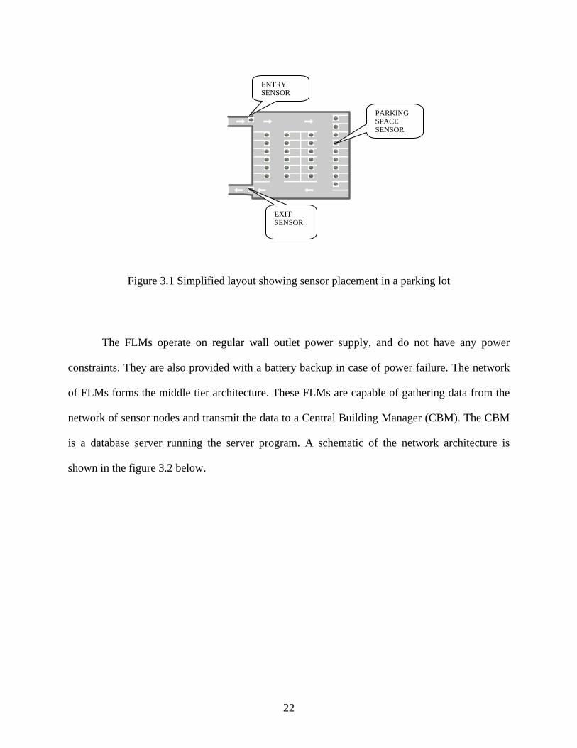
when there is any change in the sensing activity. The layout of the parking nodes in a parking lot

is shown in the figure 3.1 below. A Floor Level Manager (FLM) is assigned to each floor of the

parking garage to coordinate with the sensor units and to collect the data from them during

monitoring. The FLM is usually fixed to the ceiling of the parking garage on all floors, such that

it is equidistant from all sensor nodes on all four corners.

21

ENTRY SENSOR

PARKING SPACE SENSOR

EXIT SENSOR

Figure 3.1 Simplified layout showing sensor placement in a parking lot

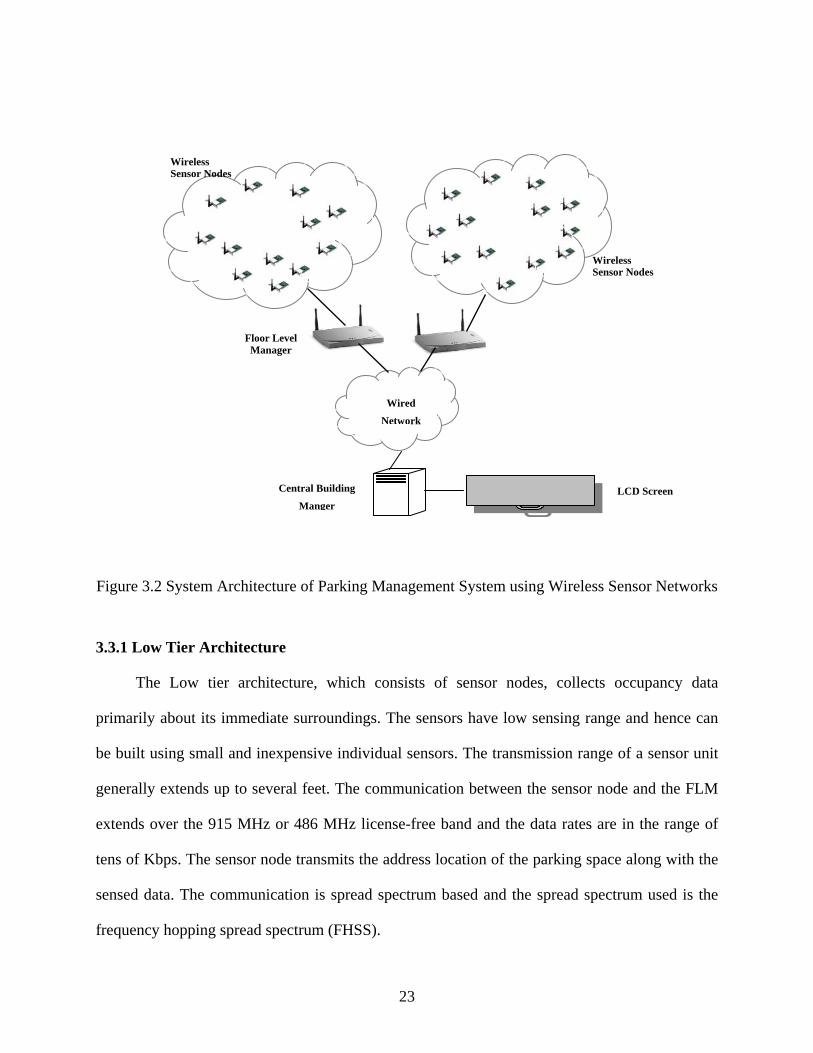
The FLMs operate on regular wall outlet power supply, and do not have any power

constraints. They are also provided with a battery backup in case of power failure. The network

of FLMs forms the middle tier architecture. These FLMs are capable of gathering data from the

network of sensor nodes and transmit the data to a Central Building Manager (CBM). The CBM

is a database server running the server program. A schematic of the network architecture is

shown in the figure 3.2 below.

22

Wireless Sensor Nodes

Wireless Sensor Nodes

Wired

Network

Central Building

Manger

Floor Level Manager

LCD Screen

Figure 3.2 System Architecture of Parking Management System using Wireless Sensor Networks

3.3.1 Low Tier Architecture

The Low tier architecture, which consists of sensor nodes, collects occupancy data

primarily about its immediate surroundings. The sensors have low sensing range and hence can

be built using small and inexpensive individual sensors. The transmission range of a sensor unit

generally extends up to several feet. The communication between the sensor node and the FLM

extends over the 915 MHz or 486 MHz license-free band and the data rates are in the range of

tens of Kbps. The sensor node transmits the address location of the parking space along with the

sensed data. The communication is spread spectrum based and the spread spectrum used is the

frequency hopping spread spectrum (FHSS).

23

3.3.2 Middle Tier Architecture

The FLMs distributed across the various floors of the parking space form the middle tier

of the network architecture. The FLMs act as sensor gateways and pass on the information from

the sensor units to the CBM, using two radios, one operating at 915 MHz to communicate with

the router nodes and the other operating at 2.4 GHz ISM band to communicate with the Central

Building Manager. The FLMs are designed to handle data rates in the range of Mbps. The

communication over the 2.4 GHz link can be based on standard protocols like IEEE 802.11b. In

addition to the FLMs, the middle tier architecture also contains two sensor nodes located at the

entrance and exit of the parking garage. These sensor nodes detect the passage of vehicles

moving in and out of the garage by sensing the deflection in the magnetic field. For this purpose

these sensor nodes are assembled with special magnetometer sensors. A simple algorithm loaded

into the sensor node increments the vehicle count when a vehicle enters and vice versa. The total

vehicles present in the parking garage can be calculated and the number of vacant spaces

available can be found, as the total number of parking spaces in a garage is known. This

additional information gives a hint of the number of vacant spaces available in the garage to the

commuter. On the other hand, the sensor nodes placed in individual parking space gives the

exact location of the free parking space to the commuter.

3.3.3 Higher Tier Architecture

The higher tier architecture consists of the Central Building Manager (CBM), which acts

as the base station to store the data values. The data from the CBM can then be displayed on

giant LCD screens, which are put for notice at the front of the parking garage for the commuters.

Another way would be to integrate data of all the CBMs located in all the parking garages

and to display the data collected through a LCD screen display at the entrance of the campus.

24

This allows a commuter to find the nearest available parking garage from the place of his

location. This procedure would be ideally suited for University campuses, which has many

parking garages.

The availability of parking space in a garage should be displayed on the LCD screen

based on current situation. When there is huge number of parking space available, the user

doesn’t need to know the location of these spaces. In such cases, it would be appropriate to

merely display the percentage of available parking space in the parking garage. In cases, where

the parking garage is nearly full, it would be ideal to display the exact location of the free

parking space. This will enable the user to park his vehicle his vehicle at the available parking

space without any haste.

With growing usage of wireless devices such as cell phones and PDAs, parking

information can also be made available to users through these devices.

25

CHAPTER 4: EXPERIMENTAL READINGS AND SIMULATION

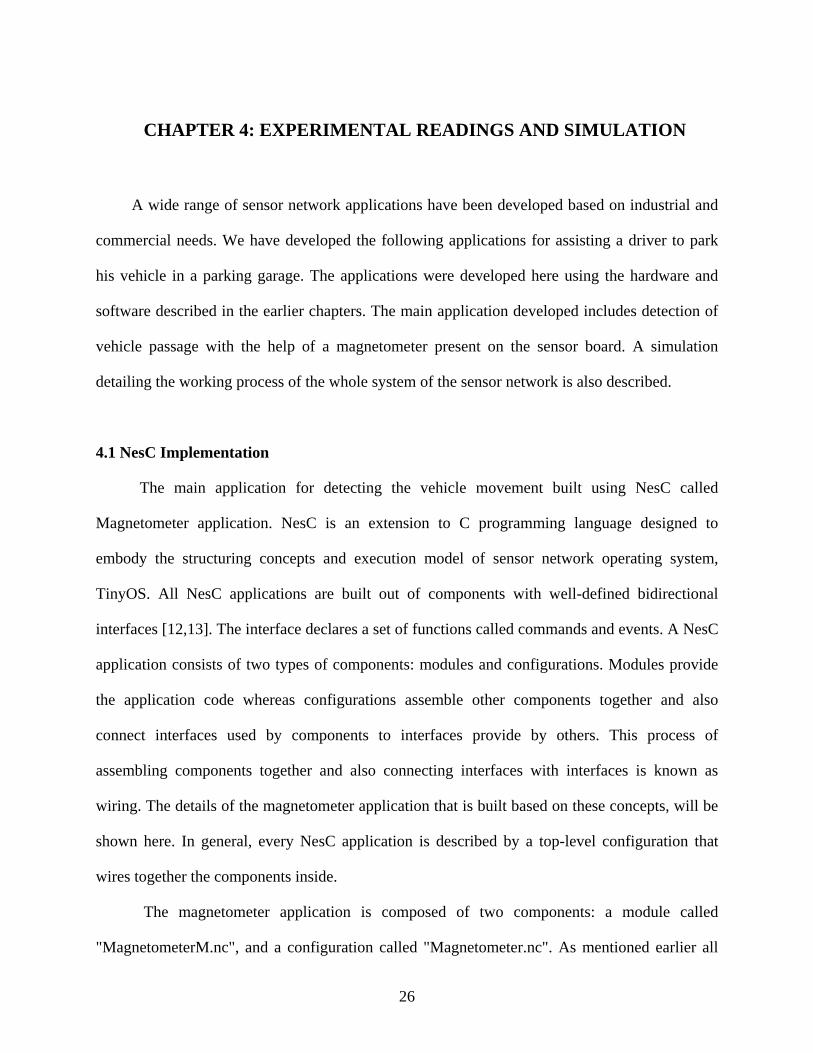
A wide range of sensor network applications have been developed based on industrial and

commercial needs. We have developed the following applications for assisting a driver to park

his vehicle in a parking garage. The applications were developed here using the hardware and

software described in the earlier chapters. The main application developed includes detection of

vehicle passage with the help of a magnetometer present on the sensor board. A simulation

detailing the working process of the whole system of the sensor network is also described.

4.1 NesC Implementation

The main application for detecting the vehicle movement built using NesC called

Magnetometer application. NesC is an extension to C programming language designed to

embody the structuring concepts and execution model of sensor network operating system,

TinyOS. All NesC applications are built out of components with well-defined bidirectional

interfaces [12,13]. The interface declares a set of functions called commands and events. A NesC

application consists of two types of components: modules and configurations. Modules provide

the application code whereas configurations assemble other components together and also

connect interfaces used by components to interfaces provide by others. This process of

assembling components together and also connecting interfaces with interfaces is known as

wiring. The details of the magnetometer application that is built based on these concepts, will be

shown here. In general, every NesC application is described by a top-level configuration that

wires together the components inside.

The magnetometer application is composed of two components: a module called

"MagnetometerM.nc", and a configuration called "Magnetometer.nc". As mentioned earlier all

26

applications require a top-level configuration file, which is typically named after the application

itself. In this case, Magnetometer.nc is the configuration for the Magnetometer application and

also the source file. The NesC compiler uses this source file "Magnetometer.nc" to generate an

executable file. On the other hand, MagnetometerM.nc provides the actual implementation of the

magnetometer application. The configuration "Magneteometer.nc" wires the

"MagnetometerM.nc" module to other components that the application requires. The entire

source code used in this application is provided in the appendix section.

4.1.1 The Magnetometer.nc Configuration

In this section we describe the components used in the "Magnetometer.nc" configuration.

configuration Magnetometer { } implementation { components Main, MagnetometerM, TimerC, LedsC, UARTComm as Comm, Mag; Main.StdControl -> MagnetometerM; Main.StdControl -> TimerC; MagnetometerM.Timer -> TimerC.Timer[unique("Timer")]; MagnetometerM.Leds -> LedsC; MagnetometerM.MagControl -> Mag; //contd. }

From the above code, we see that this configuration references a set of components viz,

Main, MagnetometerM, TimerC, LedsC, UARTComm and Mag. Main is a component that

should be present in every configuration of TinyOS application. In a similar manner, StdControl

is a common interface to initialize TinyOS components. The simple structure of StdControl is

shown below.

StdControl.nc interface StdControl { command result_t init(); command result_t start(); command result_t stop(); }

27

From the above code, it can be understood that init () is called when a component is

initialized, start () is called when the component is executed for the first time and stop () when

the component is stopped.

In the next two lines of the Magnetometer.nc code above, StdControl interface in the

Main component is wired to the StdControl interface in both Magnetometer and TimerC. TimerC

allows multiple instances of timers. Next we look at the interfaces used and provided by the

component. The relationship between interfaces is subtly represented by arrows. In general, the

component referred to on the left side of the arrow binds an interface to the component referred

on the right side. The line in the above code,

MagnetometerM.Timer -> TimerC.Timer[unique("Timer")]; is used to wire the Timer interface used by MagnetometerM to the Timer interface provided by

TimerC. In this case, the timer interface in each of the components is wired to a separate instance

of the Timer interface provided by TimerC. This allows each component to have its own timer.

In this way, one timer can fire at a certain rate to gather sensor readings while another timer of a

component fire at different rate to mange radio transmission.

4.1.2 The MagnetometerM.nc Module

The Module MagnetometerM.nc is explained as follows. module MagnetometerM { provides interface StdControl; uses { interface Timer; interface Leds; interface StdControl as MagControl; interface ADC as MagX; interface ADC as MagY; //contd. } }

28

The module above implements the StdControl interface. It also uses several interfaces like

Timer, Leds, StdControl, ADC etc. The Leds interface is used to turn on and turn off the

different LEDs on the mote. The Timer interface uses two commands – start ( ) and stop ( ) and a

fired ( ) event. The application knows that its timer has expired when it receives a fired ( ) event.

The unit of the timer interval is millisecond. As soon as the fired ( ) event is received, the

collected data is sent back.

event result_t Timer.fired() { return call MagY.getData(); } The ADC interface is used to access data from analogue-to-digital converter and the StdControl

initializes the ADC component. The module uses the StdControl interface but gives the interface

instance the name MagControl.

4.1.2.1 Wiring ADC component to sensor

In this application the ADC is wired to the magnetometer sensor as follows. This allows

the ADC channel to access the magnetometer sensor. The module uses the ADC interfaces but

gives the interface instance the name MagX and MagY. Therefore the wiring for the ADC is as

follows:

MagnetometerM.MagControl -> Mag; MagnetometerM.MagX -> Mag.MagX; MagnetometerM.MagY -> Mag.MagY;

4.1.2.2 Main Body

Next we look at the main body of the MagnetometerM.nc module. This consists of the

init (), start () and stop () commands for different interfaces. The Timer.start () creates a repeat

timer that expires for every 125 ms.

29

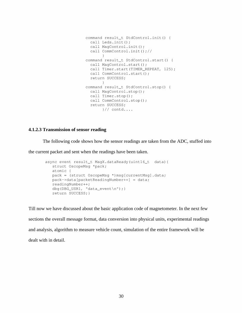
command result_t StdControl.init() { call Leds.init(); call MagControl.init(); call CommControl.init();// } command result_t StdControl.start() { call MagControl.start(); call Timer.start(TIMER_REPEAT, 125); call CommControl.start(); return SUCCESS; } command result_t StdControl.stop() { call MagControl.stop(); call Timer.stop(); call CommControl.stop(); return SUCCESS; }// contd....

4.1.2.3 Transmission of sensor reading

The following code shows how the sensor readings are taken from the ADC, stuffed into

the current packet and sent when the readings have been taken.

async event result_t MagX.dataReady(uint16_t data){ struct OscopeMsg *pack; atomic { pack = (struct OscopeMsg *)msg[currentMsg].data; pack->data[packetReadingNumber++] = data; readingNumber++; dbg(DBG_USR1, "data_event\n");} return SUCCESS;}

Till now we have discussed about the basic application code of magnetometer. In the next few

sections the overall message format, data conversion into physical units, experimental readings

and analysis, algorithm to measure vehicle count, simulation of the entire framework will be

dealt with in detail.

30

4.2 Message Format

The raw data transmitted from each node to the base station can be broken down and

analyzed as shown below here. Ten readings are combined together to form a single data packet.

Formation of each data packet

Destination address (2 bytes)

Active Message handler ID (1 byte)

Group ID (1 byte)

Payload (up to 29 bytes):

Source mote ID (2 bytes)

Sample counter (2 bytes)

ADC channel (2 bytes)

ADC data readings (10 readings of 2 bytes each)

From the format shown above, a data packet can be interpreted as follows:

Dest Handler Group Msg Source counter readings Addr ID ID len Addr channel 7e 00 0a 7d 1a 01 00 14 00 01 00 96 03 97 03 97 03 98 03 97 03 96 03 97 03 96 03 96 03 96 03

This format was used in analyzing and modifying data from the magnetometer application.

4.3 Data Conversion

In the earlier section, we have described the structure of the raw data gathered from the

sensor networks. A user interface is required to view the sensor readings. The raw ADC readings

can be converted to suitable engineering units based on the parameter measured. The conversion

program is written in C. This program enables to recognize and interpret data packets in a

standardized format. (Wireless systems for environmental applications) The data can be viewed

31

in the cygwin shell itself. The data can be exported to spreadsheet form to build graphs of the

values. The data conversion program has a set of basic functions for data pre-processing and

post-processing operations. Data pre-processing is to ensure the quality of the data for analysis.

Data post-processing is mainly for the presentation of analytical results. The function convert ()

converts sensor readings from raw ADC counts to human-friendly engineering units. The

function connect () is used to connect the current set of readings to the PostgresSQL database. In

our application the data gathered needs to be accessed to provide information to the drivers

entering the parking lot. Hence an application which features a live data feed component in

which the data can be viewed as the information is being collected is necessary. PSQL is an

Object-Relational Database Management System (ORDBMS). PSQL approaches data with an

object-relational model, and is capable of handling complex routines and rules. Each set of data

is time-stamped and also stamped with the node-id of the node that collects that data. The data is

retrieved from the central database by sending a query, which is a PSQL command. Listen () is a

function that listens to the serial port and outputs the sensor data in human readable form. When

a user runs a query, the information is taken and a SQL query is generated based upon the user

request and the corresponding data is exported. The code that does the function of convert,

connect and listen is shown in the Appendix II section.

4.4 Experiments and Data Analysis

For all the implementations, the following hardware and software were used:

Hardware (from Crossbow) – one MICA2 Sensor node, one MTS310CA Sensor board and a

MIB510 Interface board. Two AA industrial alkaline batteries were used to power the interface

board to which the sensor node and sensor board were connected. A standard Laptop with

32

configuration of 1.99 GHz processor and 256MB RAM was used for logging values. A RS-232

cable is used to connect the Interface board unit with the Laptop.

Software – NesC is the programming language used to write the magnetometer application.

These applications can be run from a Cygwin shell, which works with all versions of Windows

since Windows 95.

A Set of experiments is performed using the hardware and software described above to

detect the movement of vehicles. In the following experiments the node is embedded with the

magnetometer application for detecting vehicular motion. The Sensor node and Sensor board are

fixed to the 51-pin connector present on both sides of the interface board. Two AA batteries

power the sensor node, which powers the whole combination. The whole hardware combination

is connected to a Laptop using a RS-232 cable. The block diagram of the whole experiment setup

is shown in the figure 4.1 below.

Interface Board RS-232

Sensor

Sensor Node

Laptop

Figure 4.1 Block Diagram of Experimental Setup

In our first experiment, the main objective is to detect vehicle presence when the vehicle

passes over the sensor. In this case, the hardware combination is kept directly at the center of the

lane of interest, for the vehicles to move over. As explained in the network architecture, two

nodes placed at the entrance and exit keeps track of the vehicles entering and leaving the parking

lot. The sole purpose of this experiment is to emulate the performance of the entry-exit sensors.

33

The measurements of the sensor node simply give single hill patterns when a car passes by. This

is shown in figure 4.2. We assume the vehicle velocity to be a max of 25 MPH (around 11.176

m/s) and that an engine block of the car is at least 60 cm long and 3 samples need to be taken

during a vehicle pass-through. The sampling frequency needed would then be 55 Hz (11.17 m/s

* 3/60cm).

Figure 4.2 Detection of a single moving car

In our next experiment the analysis shifts to the condition where two cars move over the

sensor, bumper-to-bumper. In such cases, getting at least three samples during the movement of

each engine block is necessary. The detection of two vehicles graphically moving bumper-to

bumper is shown in figure 4.3.

34

Figure 4.3 Detection of two moving cars in a bumper-to-bumper fashion

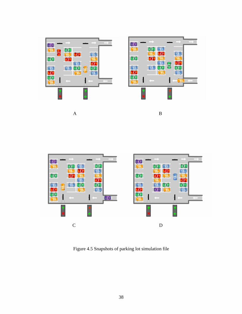
4.5 Simulation of the Parking Management System

In the earlier sections we have seen the implementation of a single sensor node to detect

the movement of vehicles. The simulation described in this section gives a glimpse of the actual

layout of sensor nodes in a parking lot, their collaborative functioning, data gathering and

information display to a driver entering the lot. Considering the time and cost factors, simulation

is an attractive alternative to experimental deployment of wireless sensor network applications,

which are in development. The simulation is developed using Macromedia Flash MX

Professional 2004 package, in accordance to the architecture of the parking management system

described in chapter 3. The major aim of this simulation development is to replicate the working

of the entire system and also to display information to the driver based on the data gathered from

the sensors. The simulation developed here models the behavior, form and visual appearance of a

35

simple real world situation. The real world situation shows cars entering the parking lot and the

driver clearly able to find empty parking spaces from the information display boards. The clear

objective of this simulation approach is obtained by using Flash programming. Flash offers

ActionScript, which is an object-oriented programming language based on the same standard as

JavaScript.

4.5.1 Algorithm Design

The algorithm design of the simulation framework is shown in the figure below. It is a simple

step-by-step procedure of the actual implementation of the system. In this case a car enters the

parking lot after looking for available space form the LED display positioned at the front. Once

the car enters the parking lot, a sensor node positioned at the entrance detects its movement and

sends the data to the central base-station. The base station increments the count value of the total

parked cars in the lot by one unit. The change in the total count value is appropriately transmitted

to the LED displays, which shows the change. Once the car is inside the parking lot, it looks for

display screens located at the entrance of parking rows. The screens show the availability of

parking spaces in that parking row by simple signs. Once the driver finds that the parking row

has empty space(s) to park, he moves in to park his vehicle in that empty parking spot. A sensor

node positioned at the center of the parking spot detects the vehicle presence and immediately

informs to the base-station. The base-station keeps track of the count of vehicles, actually parked

in and changes information on the display boards. A simple occupancy sensor can identify the

vehicle presence in the parking spot. When the vehicle leaves the parking spot, the status is

immediately transmitted to the base-station. The exit tracking process is similar to entry tracking

process except that the count value is decremented, when the vehicles leave the parking lot.

36

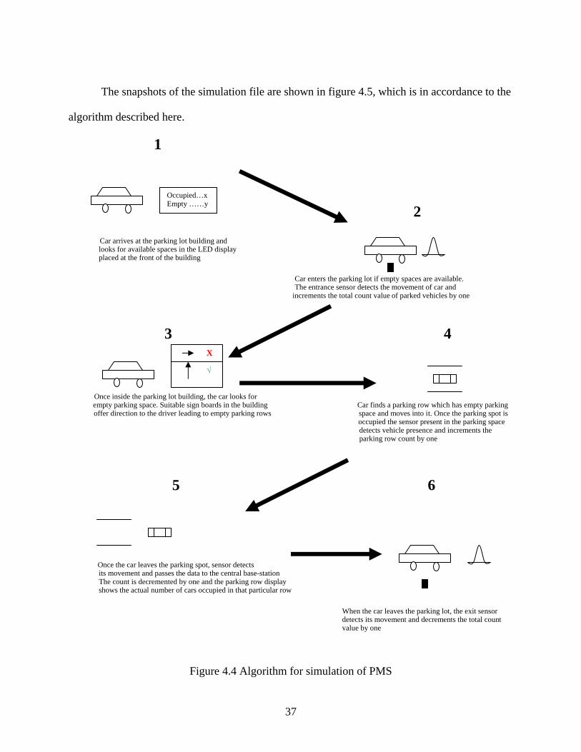
The snapshots of the simulation file are shown in figure 4.5, which is in accordance to the

algorithm described here.

1

2 Occupied…x Empty ……y

Car arrives at the parking lot building and looks for available spaces in the LED display placed at the front of the building

Car enters the parking lot if empty spaces are available.

The entrance sensor detects the movement of car and increments the total count value of parked vehicles by one

3 4

X

√

Once inside the parking lot building, the car looks for empty parking space. Suitable sign boards in the building Car finds a parking row which has empty parking to the driver leading to empty parking rows space and moves into it. Once the parking spot is offer direction occupied the sensor present in the parking space d parking row count by one

etects vehicle presence and increments the

5 6

Once the car leaves the parking spot, sensor detects The count is decremented by one and the parking row display

its movement and passes the data to the central base-station

shows the actual number of cars occupied in that particular row

When the car leaves the parking lot, the exit sensor detects its movement and decrements the total count value by one

Figure 4.4 Algorithm for simulation of PMS

37

A B

C D

Figure 4.5 Snapshots of parking lot simulation file

38

CHAPTER FIVE: CONCLUSION

Parking Management System using wireless sensor networks has tremendous growth and

opportunity in the coming years. Many Parking lots in the country are getting automated to ease

the tension of peak hour traffic. With growing advances in communication technology and

Internet, this application will be one of the services to rely on. However realization of this project

needs to satisfy the constraints introduced by factors like fault tolerance, scalability and

hardware. The low-level energy constraints of the sensor nodes combined with the data delivery

requirements leave a clearly defined energy budget for all other services. Tight energy bounds

and the need for predictable operation guide the development of application architecture and

services. This small research work can add some weight to this sensor network field. This research

project by itself is not a complete one and requires various other requirements to meet completion.

39

APPENDIX A

MAGNETOMETER APPLICATION

40

includes OscopeMsg; configuration Magnetometer { } implementation { components Main, MagnetometerM, TimerC, LedsC, UARTComm as Comm, Mag; Main.StdControl -> MagnetometerM; Main.StdControl -> TimerC; MagnetometerM.Timer -> TimerC.Timer[unique("Timer")]; MagnetometerM.Leds -> LedsC; MagnetometerM.MagControl -> Mag; MagnetometerM.MagX -> Mag.MagX; MagnetometerM.MagY -> Mag.MagY; //MagnetometerM.ADC -> Accel; MagnetometerM.CommControl -> Comm; MagnetometerM.ResetCounterMsg -> Comm.ReceiveMsg[AM_OSCOPERESETMSG]; MagnetometerM.Send -> Comm.SendMsg[AM_OSCOPEMSG]; } includes OscopeMsg; includes sensorboard; module MagnetometerM { provides interface StdControl; uses { interface Timer; interface Leds; //interface StdControl as SensorControl; interface StdControl as MagControl; //interface ADC; interface ADC as MagX; interface ADC as MagY; interface StdControl as CommControl; //interface SendMsg as DataMsg; interface SendMsg as Send; interface ReceiveMsg as ResetCounterMsg; } } implementation { uint8_t packetReadingNumber; uint16_t readingNumber; TOS_Msg msg[2]; uint8_t currentMsg; norace TOS_MsgPtr msgPtr; norace TOS_MsgPtr oldmsgPtr; norace char msgIndex; task void SendTask() { call Send.send(TOS_UART_ADDR, 29, msgPtr); } command result_t StdControl.init() { call Leds.init(); call Leds.yellowOff(); call Leds.redOff(); call Leds.greenOff(); call MagControl.init(); call CommControl.init(); atomic { currentMsg = 0; packetReadingNumber = 0; readingNumber = 0; } dbg(DBG_BOOT, "OSCOPE initialized\n");

41

return SUCCESS; } command result_t StdControl.start() { //call SensorControl.start(); call MagControl.start(); call Timer.start(TIMER_REPEAT, 125); call CommControl.start(); return SUCCESS; } command result_t StdControl.stop() { // call SensorControl.stop(); call MagControl.stop(); call Timer.stop(); call CommControl.stop(); return SUCCESS; } task void dataTask() { struct OscopeMsg *pack; atomic { pack = (struct OscopeMsg *)msg[currentMsg].data; packetReadingNumber = 0; pack->lastSampleNumber = readingNumber; } pack->channel = 1; pack->sourceMoteID = TOS_LOCAL_ADDRESS; if (call Send.send(TOS_UART_ADDR, sizeof(struct OscopeMsg), &msg[currentMsg])) { atomic { currentMsg ^= 0x1; } call Leds.yellowToggle(); } } async event result_t MagX.dataReady(uint16_t data){ struct OscopeMsg *pack; atomic { pack = (struct OscopeMsg *)msg[currentMsg].data; pack->data[packetReadingNumber++] = data; readingNumber++; dbg(DBG_USR1, "data_event\n");} return SUCCESS; } async event result_t MagY.dataReady(uint16_t data) { struct OscopeMsg *pack; atomic { pack = (struct OscopeMsg *)msg[currentMsg].data; pack->data[packetReadingNumber++] = data; readingNumber++; dbg(DBG_USR1, "data_event\n"); if (packetReadingNumber == BUFFER_SIZE) { post dataTask(); } } if (data > 0x0300) call Leds.redOn(); else call Leds.redOff(); return SUCCESS; } event result_t Send.sendDone(TOS_MsgPtr sent_msgptr, result_t success){ }

42

event result_t Timer.fired() { return call MagY.getData(); } event TOS_MsgPtr ResetCounterMsg.receive(TOS_MsgPtr m) { atomic { readingNumber = 0; } return m; } } include "../xdb.h" #include "../xsensors.h" typedef struct { uint16_t vref; uint16_t thermistor; uint16_t light; uint16_t mic; } XSensorMTS300Data; typedef struct { uint16_t vref; uint16_t thermistor; uint16_t light; uint16_t mic; uint16_t accelX; uint16_t accelY; uint16_t magX; uint16_t magY; } XSensorMTS310Data; uint16_t mts300_convert_light(uint16_t light, uint16_t vref) { float Vbat = xconvert_battery_mica2(vref); uint16_t Vadc = (uint16_t) (light * Vbat / 1023); return Vadc; } float mts310_convert_mag_x(uint16_t data,uint16_t vref) { // float Vbat = mts300_convert_battery(vref); // float Vadc = data * Vbat / 1023; // return Vadc/(2.262*3.0*3.2); float Magx = data / (1.023*2.262*3.2); return Magx; }

43

APPENDIX B

Data Conversion and Display

44

/** * Computes the ADC count of the Magnetometer - for Y axis reading into * Engineering Unit (mgauss), no calibration * * SENSOR Honeywell HMC1002 * SENSITIVITY 3.2mv/Vex/gauss * EXCITATION 3.0V (nominal) * AMPLIFIER GAIN 2262 * ADC Input 22mV/mgauss * */ float mts310_convert_mag_y(uint16_t data,uint16_t vref) { // float Vbat = mts300_convert_battery(vref); // float Vadc = (data * Vbat / 1023); // return Vadc/(2.262*3.0*3.2); float Magy = data / (1.023*2.262*3.2); return Magy; } /** MTS300 Specific outputs of raw readings within an XBowSensorboardPacket */ void mts300_print_raw(XbowSensorboardPacket *packet) { XSensorMTS300Data *data = (XSensorMTS300Data *)packet->data; printf("mts300 id=%02x vref=%04x thrm=%04x light=%04x mic=%04x\n", packet->node_id, data->vref, data->thermistor, data->light, data->mic); } /** MTS300 specific display of converted readings from XBowSensorboardPacket */ void mts300_print_cooked(XbowSensorboardPacket *packet) { XSensorMTS300Data *data = (XSensorMTS300Data *)packet->data; printf("MTS300 [sensor data converted to engineering units]:\n" " health: node id=%i parent=%i\n" " battery: = %i mv \n" " temperature: =%0.2f degC\n" " light: = %i mv\n" " mic: = %i ADC counts\n", packet->node_id, packet->parent, xconvert_battery_mica2(data->vref), xconvert_thermistor_temperature(data->thermistor), mts300_convert_light(data->light, data->vref), data->mic); printf("\n"); } /** * Logs raw readings to a Postgres database. * * */ void mts300_log_raw(XbowSensorboardPacket *packet) { XSensorMTS300Data *data = (XSensorMTS300Data *)packet->data; char command[512]; char *table = "mts300_results"; sprintf(command, "INSERT into %s " "(result_time,nodeid,parent,voltage,temp,light)" " values (now(),%u,%u,%u,%u,%u)", table, packet->node_id, packet->parent, data->vref, data->thermistor, data->light );

45

xdb_execute(command); } /** MTS310 Specific outputs of raw readings within an XBowSensorboardPacket */ void mts310_print_raw(XbowSensorboardPacket *packet) { XSensorMTS310Data *data = (XSensorMTS310Data *)packet->data; printf("mts310 id=%02x vref=%4x thrm=%04x light=%04x mic=%04x\n" " accelX=%04x accelY=%04x magX=%04x magY=%04x\n", packet->node_id, data->vref, data->thermistor, data->light, data->mic, data->accelX,data->accelY, data->magX, data->magY); } void mts310_print_cooked(XbowSensorboardPacket *packet) { XSensorMTS310Data *data = (XSensorMTS310Data *)packet->data; printf("MTS310 [sensor data converted to engineering units]:\n" " health: node id=%i parent=%i\n" " battery: = %i mv \n" " temperature=%0.2f degC\n" " light: = %i ADC mv\n" " mic: = %i ADC counts\n" " AccelX: = %f g, AccelY: = %f g\n" " MagX: = %0.2f mgauss, MagY: =%0.2f mgauss\n", packet->node_id, packet->parent, xconvert_battery_mica2(data->vref), xconvert_thermistor_temperature(data->thermistor), mts300_convert_light(data->light, data->vref), data->mic, xconvert_accel(data->accelX), xconvert_accel(data->accelY), mts310_convert_mag_x(data->magX,data->vref), mts310_convert_mag_y(data->magY,data->vref) ); printf("\n"); }

46

LIST OF REFERENCES [1] I.F. Akyildiz, W. Su, Y. Sankarasubramaniam, and E. Cayirci, “A Survey on Sensor

Networks,” IEEE Communication Magazine, August 2002

[2] G. Pottie and W. Kaiser, “Wireless Integrated Network Sensors,”Communications of the

ACM, vol. 43, pp. 51–58, May2000.

[3] J.M. Kahn, R.H. Katz, and K.S.J. Pister, “Next Century Challenges: Mobile Networking

for “Smart Dust”,” MobiCom’99, Seattle, Washington, 1999.

[4] A. Mainwaring, J. Polastre, R. Szewczyk, D. Culler, and J. Anderson, “Wireless Sensor

Network for Habitat Monitoring,” ACM WSNA’02, Atlanta, Georgia, USA, September

2002.

[5] Jason Lester Hill, “System Architecture for Wireless Sensor Network,” PhD Dissertation

Dissertation, University of California, Berkeley, 2003.

[6] G.J. Pottie, and W.J. Kaiser, “Wireless Integrated Network Sensors,” Communication of

the ACM, May 2000.

[7] Y. Kawahara, M. Minami, H. Morikawa, T. Aoyama: "Design and Implementation of a

Sensor Network Node for Ubiquitous Computing Environment," In Proceedings of

IEEE Semiannual Vehicular Technology Conference(VTC2003-Fall), Orlando,

USA, October 2003.

[8] J. Hill, R. Szewczyk, A. Woo, S. Hollar, D. E. Culler, and K. S. J. Pister. System

architecture directions for networked sensors. In Architectural Support for Programming

Languages and Operating Systems, pages 93–104, Boston, MA, USA, Nov. 2000.

[9] MICA http://www.xbow.com/Products/Product pdf files/Wireless pdf/MICA.pdf

[10] Michael J. Caruso, Lucky S. Withanawasam, “Vehicle Detection and Compass

47

Applications using AMR Magnetic Sensors, Honeywell, SSEC,

www.ssec.honeywell.com

[11] Honeywell Corporation, HMC 1001 / 1002 / 1021 / 1022, 1- and 2- Axis magnetic

Sensors. http://www.ssec.honeywell.com/magnetic/datasheets/hmc1001-2_1021-2.pdf

[12] TinyOS website: http://tinyos.net

[13] TinyOS Tutorial: http://www.tinyos.net/tinyos-1.x/doc/tutorial/

[14] N. Xu, S. Rangwala, K.K. Chintalapudi, D. Ganesan, A. Broad, R. Govindan,

and D. Estrin, “A Wireless Sensor Network for Structural Monitoring,” ACM

SenSys’04, Baltimore, Maryland, USA, November 2004.

48