Design and Implementation of a Sensor Network System for Vehicle Tracking andAutonomous Interception

DRAFT DRAFT DRAFT DRAFT DRAFT DRAFT DRAFTDo not distribute without written permission from the authors.

DRAFT DRAFT DRAFT DRAFT DRAFT DRAFT DRAFT

Cory Sharp Shawn Schaffert Alec Woo Naveen Sastry Chris KarlofShankar Sastry David Culler

{cssharp,sms,awoo,nks,ckarlof,sastry,culler}@eecs.berkeley.edu

Abstract

We describe the design and implementation of PEG, a net-worked system of distributed sensor nodes that detects anuncooperative agent called theevader and assists an au-tonomous robot called thepursuer in capturing the evader.PEG requires services such as leader election, routing, net-work aggregation, and closed loop control. Instead of usinggeneral purpose distributed system solutions for these ser-vices, we employ whole-system analysis and rely on spatialand physical properties to create simple and efficient mech-anisms. We believe this approach advances sensor networkdesign, yielding pragmatic solutions that leverage physicalproperties to simplify design of embedded distributed sys-tems.

We deployed PEG on a 400 square meter field using 100sensor nodes, and successfully intercepted the evader in allruns. While implementing PEG, we confronted practical is-sues such as node breakage, packaging decisions, in situ de-bugging, network reprogramming, and system reconfigura-tion. We discuss the approaches we took to cope with theseissues and share our experiences in deploying a large sensornetwork system.

1 Introduction

The problem of vehicle tracking with autonomous intercep-tion provides a concrete setting in which to advance sensornetwork and control system design. In our case, wireless sen-sor nodes containing magnetometers are distributed through-out a large physical area to form a diffuse sensing field. Anuncooperative agent, theevader, enters and moves within thisarea, where it is detected by the magnetometers. Unlike en-vironmental monitoring, it is not enough to obtain measure-ments of the physical disturbance caused by evader; we wantto process the readings within the network and take actionin a timely matter. Thepursuer, a cooperative mobile agent,enters the field and attempts to intercept the evader using in-formation obtained from the sensor network and its own au-

tonomous control capabilities.Local signal processing can be performed at each node to

distill higher-level events given magnetic-field measurementsdue to motions of multiple vehicles. Clusters of nodes thatsense sufficiently strong events can collectively compute anestimate of the position of the vehicle causing the distur-bance. These potentially noisy estimations from multiple ob-jects must be disambiguated and used to make continual pur-suer course corrections.

The autonomous interception problem concretely mani-fests many of the capabilities envisioned for sensor net-works [10, 25], including several levels of in-network pro-cessing, routing to mobile agents, distributed coordination,and closed-loop control. We address these issues in termsof the whole system design, rather than as isolated subprob-lems. Indeed, this whole-system view yields pragmatic solu-tions that are more simple than what is generally found in theliterature for individual subproblems.

We built and demonstrated a working purser/evader systemcomprising a field of 100 motes spread over a400m2 area inJuly 2003. The evader was a four-wheeled robot driven bya person using remote control. The pursuer was an identicalrobot with laptop-class resources. This paper describes thedesign, implementation, and experience with PEG. Section 2discusses our overall design philosophy with respect to re-lated work. Section 3 describes the application, the hardwareplatform, and the overall software system design. Section 4describes the in-network processing components for local de-tection and aggregation into a position estimate. Section 5focuses on effective mobile-to-mobile routing, including ef-fective tree formation and efficient landmark routing. Section6 describes the design of the navigation and control of thepursuer. Section 7 evaluates our system design, and Section 8outlines several of the experiences that have an impact on theoverall system design and implementation.

Our main contributions are:

• We describe the design and implementation of PEG, anetworked system of distributed sensor nodes that de-

Figure 1: Illustration of an intruder interception system us-ing sensor networks to detect the intruder (arrow) and con-vey such information to the pursuing robots. Each pursuermatches the sensor data to its local map for path estimationand interception of the intruder.

tects an evader and aids a pursuer in capturing the evader.

• We employ whole-system analysis and utilize spatialand physical properties to design efficient and simpledistributed algorithms. We believe this approach is ap-plicable to a variety of applications.

• We demonstrate one of the first operating large-scaletracking and pursing system that uses computationallyand bandwidth limited sensor nodes.

• We share practical advice for deploying large sensornetwork applications, including package design, debug-ging techniques, and high-level network managementservices.

2 Approach

Variants of the pursuer-evader problems have been well stud-ied from a theoretical point of view [21, 30] and have beenused for distributed systems research [35]. Sophisticated al-gorithms [22, 26] have been developed to associate readingswith logical tracks of multiple objects. Elaborate data struc-tures are used to deal with dynamic track creation and elimi-nation of potential tracks caused by input noise. In addition,there is work [13] on closed loop control for the autonomouspursuer starting with various assumptions about what infor-mation is provided to the robot.

The early work on wireless sensor nets observed that dis-tributing intelligence throughout the sensor array dramati-cally simplified the tracking problem [25]. When dense sens-ing is employed, each patch of sensors only has to deal witha few objects in a limited spatial region. Signal processing isgreatly simplified because the sensors are close to the source,

so the SNR is high. Physical constraints, such as speed ofmovement, allow for low-level filtering of false positives.

Others have studied a decentralized form of the problemwhere object tracking, classification, and path estimation areperformed by a network of wireless sensors [6, 16]. In thisformulation, sensing and detection are performed by localcollaborative groups, each responsible for tracking a singletarget. The solution is cast in traditional distributed systemterms with an explicit representation of the group associatedwith each object. Movement of the object involves nodesjoining and leaving the group. Leader election is performedso that a particular node represents the object at any point intime and typically as the root of the collaborative signal pro-cessing. Recent work optimizes a single objective functionthat combines the cost of signal processing and tracking withthe benefits of obtaining the given data [38]. Sophisticatedprogramming environments have been proposed [5] to main-tain the distributed data structure representing each logicalentity and the set of nodes associated with its track. Unsur-prisingly, these studies suggest that quite powerful nodes arerequired to perform distributed tracking. In addition, Welshand Mainland have proposed a higher-level programming en-vironment that uses abstract regions to simplify developmentof sensor applications [36]. Recently, other researchers havebegun to focus on the use of very simple outputs from densenetworks of sensors. For example, Aslam et al. [3] exploretracking where each sensor reports only a single bit of infor-mation of whether the disturbance is getting closer.

We adopt a light-weight approach that stems from two keyobservations. First, the autonomous interception problem ad-mits a natural hierarchy. The lowest-tier of nodes, whichare the most numerous and most resource constrained, areresponsible for simple detection functions and for providingdistilled information to a higher-tier. The higher-tier is ca-pable of doing more substantial processing and initiating ac-tions based on the information. In a basic tracking problem,the higher tier might include computer-controlled cameras,whereas in the interception problem it is a mobile pursuer. El-ements in the lower tier generally do not need to know muchabout the track or the identity of the object, as their behav-ior does not change based on that information. The robotsare power intensive and require substantial local processing,hence they are a natural point of concentrated processing.

Second, in-network processing at the lowest tier is essen-tial to conserve bandwidth, thereby reducing contention andkeeping notification latency low. The processed results neednot be perfect as they will be further analyzed by the highertier. For example, an inconsistent leader election may causetwo closely related position estimations for an object at nearlythe same time. This is easily addressed in the higher levelprocessing. Inconsistency is far more benign here than in thesettings where distributed consensus is typically used, for ex-ample to avoid multiple financial transactions [4, 8].

2

Calibration &Sensing

Leader Election &Data Aggregation

Data Filtering InterceptionPlanning

PursuerNavigation

Route to Mobile Pursuer

Nodes near evader

Pursuer

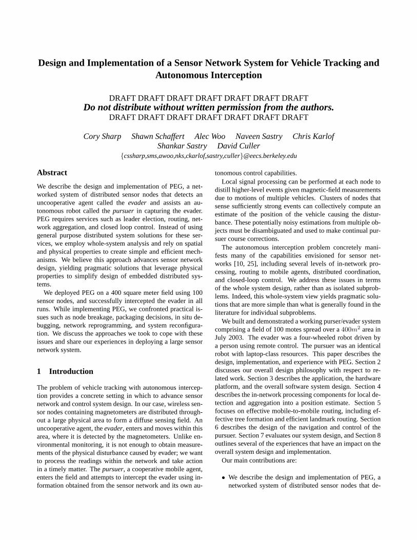
Figure 2: Logical flow of information in PEG. After the nodescalibrate their sensors, they listen for events in the network.When events are sensed near several nodes, a leader is electedto aggregate the data into one packet. This packet is routed tothe moving pursuer via multi-hop routing. After data filteringand interception planning, the pursuer chases the evader.

3 System Architecture

To provide pursuers with accurate detection events quicklyand often, we developed services for detection, routing, dataprocessing, and pursuit. We provide a sense of the overall in-formation flow and describe the constituent system services.Additional issues of power management and authenticationand encryption are beyond the scope of this paper.

3.1 Software Services

Figure 2 illustrates the information flow from the lower-tiersensing field to the higher-tier processing unit at the pursuer.The sensor network detects the evader and routes this infor-mation to the pursuer, and the pursuer acts on this data tointercept the evader. Figure 3 shows the overall system ar-chitecture of the services required to implement PEG. Thesensor tier basically performs two high-level services: self-localization and vehicle detection. The first core service, lo-calization, is used to build a coordinate system of the entirenetwork upon which the pursuer can map the collected de-tection events to meaningful physical locations. Ad-hoc self-localization is achieved using time-of-flight ultrasonic rang-ing technology with anchor-based localization algorithms.The system architecture supports self-localization, but it wasnot used in the live demonstration due to sporadic errors; thisis redressed in later work [1].

When a vehicle is present, the sensing and detection com-ponent (Section 4.2) of nearby nodes will trigger detectionevents and invoke the leader election algorithm (Section 4.4)for data aggregation. The process of leader election is real-ized over a tuple-space neighborhood service (Section 4.3).The elected leader will propagate the aggregated data to thepursuers using landmark routing, which operates over a sim-ple tree building mechanism (Section 5).

When sensor readings reach the pursuer, the pursuer usesan entity disambiguation service to determine the cause ofthe event: the evader, the pursuer, or noise. Sensor readings

Path Following Pursuit Services

Purs

uer

Arc

hite

ctur

e

Interception Planning Path Planning

Pursuer Position Estimation Estimation Services

Entity Disambiguation Evader Position Estimation

Application ServicesLocalization Leader Election and Aggregation

Sens

or N

etw

ork

Arc

hite

ctur

e

Landmark Routing Tree Building Node Management Network ServicesNetwork Reprogramming Config Neighborhood

Ranging Sensing and Entity Detection Intra-moteservicesHardware Abstraction Messaging

Figure 3: Hardware and functional division of services. Thedotted line separates services running on the pursuer from ser-vices running in the sensor network.

that are determined to correspond to the evader are sent to theevader position estimation service. The pursuer position esti-mation service uses data from the GPS unit to determine anestimate of the pursuer position. Estimates of the position ofthe pursuer and evader are sent to the interception service,which generates a interception destination for the pursuer.This destination is processed by the path planning service togenerate a feasible route. Finally, the route is submitted to thepath following service that tightly controls the pursuer alongthis route. These mechanisms are further developed in Sec-tion 6.

Beside the core functionally required for PEG, new sys-tem services are also implemented to ease the difficulty inmanaging and configuring the network at the time of deploy-ment. The Config component allows run-time configurationof system parameters that are useful for system tunings. Thenode management component is used for node identification,debugging, and network-wide power cycle management. Fi-nally, network reprogramming allows rapid reprogrammingthe entire system over the wireless medium, which is valuablefor rapid update of code image. We discuss these deploymentissues in Section 8.

3.2 Sensor Tier Platform

The sensor tier of our system consists of Berkeley Mica2Dotmotes [14], a quarter-sized unit with an 8-bit 4 MHz AtmelATMEGA128L CPU with 128 kB of instruction memory and4 kB of RAM. Its radio is a low power Chipcon CC1000radio that delivers about 2 kB/s application bandwidth witha maximum communication range of around thirty metersfor our particular antenna and environment. Each node usesa magnetometer to detect changes in a magnetic field, pre-sumably caused by a nearby moving vehicle. An ultrasoundtransceiver at 25kHz is used for time-of-flight ranging. A re-

3

Exposed components

Watertight compartment

Ultrasound

Battery

Collision absorption

CPU / RadioMag Sense

Power

Reflector

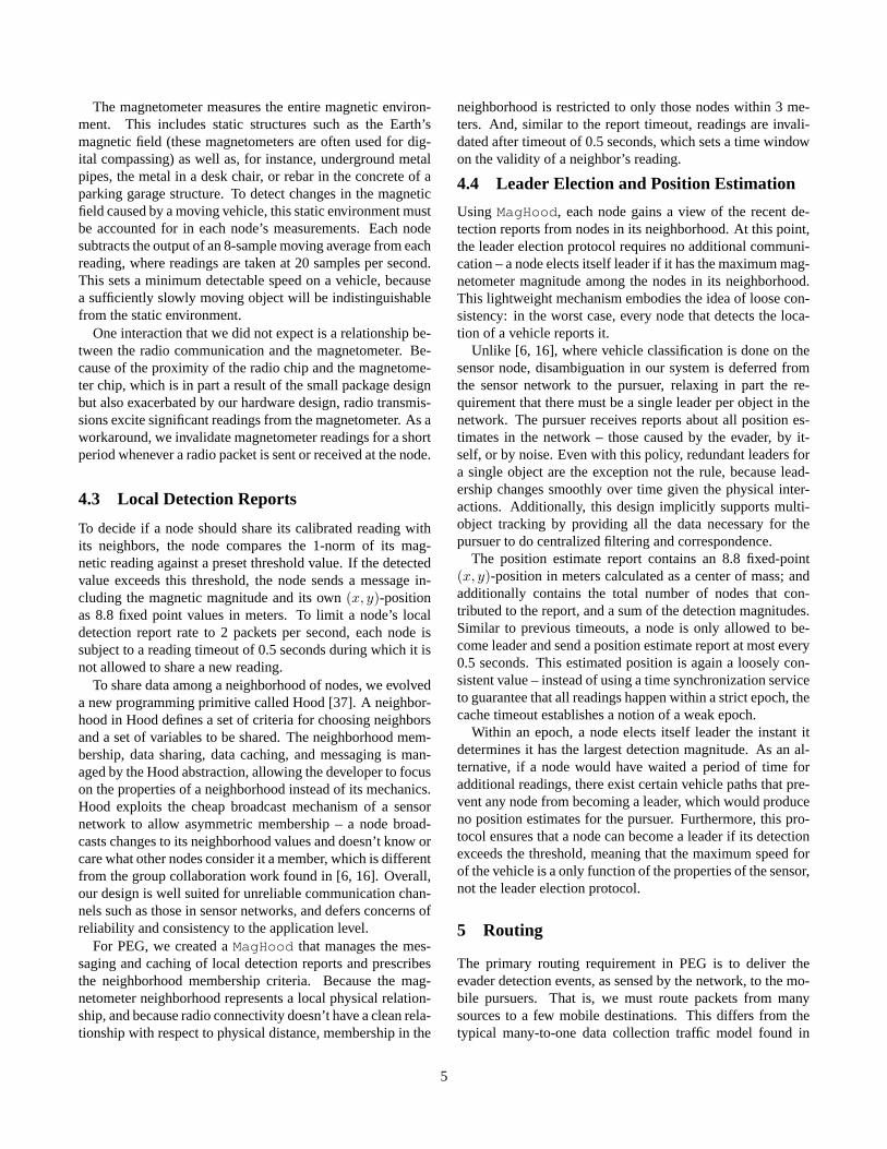
Figure 4: Photograph of a PEG sensor deployed in the fieldon the day of the demonstration (left), and a schematic of itsbasic elements (right).

flector cone is situated above the transceiver to diffuse theultrasonic waves for omni-directional ranging which signifi-cantly reduces the ranging radius to about 2 meters.

Figure 4 shows the complete packaging of a sensor node.At the bottom of the node is a base that secures the node tothe ground and extends it a few inches above the ground. Thebattery, voltage conversion board, magnetic sensor, and theMica2Dot are all protected by the plastic enclosure. The sideof the enclosure has a hole that allows a quarter-wavelengthpiano wire antenna to be connected to the Mica2Dot. Theonly sensor exposed is the ultrasound transceiver at the top,with the cone securely mounted above it. The complete pack-aging is robust against impact from vehicles, and the spring atthe base keeps the node upright even after collisions to elevatethe node a few inches above the ground plane for effective ra-dio communication.

All nodes at the sensor tier run TinyOS [14], an event-driven operating system for networked applications in wire-less embedded systems. The implementation of all the coreservices shown in Figure 3 consumes about 60 kB of programmemory and about 3 kB of RAM.

3.3 Higher Tier Platform

Our ground robots are essentially mobile off-road laptopsequipped with GPS. Each robot runs Linux on a 266 MHzPentium2 CPU with 128 MB of RAM, 802.11 wireless ra-dio, a 20 GB hard drive, all-terrain off-road tires, a motor-controller subsystem, and high-precision differential GPS.All the higher-tier services shown in Figure 3 run on this plat-form. The GPS typically provides estimates every 0.1 sec-onds with an accuracy of about 0.02 meters. The top speed ofthe robot is about 0.5m/s, with independent velocity controlfor each wheel. In our deployment, we used one pursuer andone evader, each the same model robot.

4 Vehicle Detection

Detecting a vehicle in the network begins with a node gath-ering and processing data leading up to the formation of aposition estimate report. In this section, we show how a band-width analysis of the overall system drives the design of ourphases of vehicle detection.

4.1 Bandwidth-Driven Design

We design our sensor network to provide full, redundant sen-sor coverage – for sensors placed in a grid, a vehicle excitesat least four and up to nine sensors. From this coverage re-quirement, we design the rest of the detection system withan understanding of the impact of low-level decisions on re-gional bandwidth limits.

Presuming a local aggregate bandwidth of 40 packets persecond, a single node can provide up to four reports per sec-ond before a region of nine nodes saturates the shared chan-nel. If each node sends these detection events, the local chan-nel will be saturated leaving no bandwidth for other commu-nications such as routing these readings to the pursuer. Ad-ditionally, as more vehicles are added to the system, routingthe data will increasingly tax the bandwidth of the system.Clearly, we must use some techniques to conserve bandwidth.

We use local aggregation to reduce many detection eventsinto one position report, We allocate half the total band-width for exchanging local detection reports and the remain-ing bandwidth for system wide behaviors such as routing po-sition estimates to pursuers. Even though sharing local de-tections uses a significant portion of the local bandwidth, thepursuer still receives frequent position updates. We decom-pose this overall process into three distinct phases: calibra-tion and sensing, local detection reports, and leader electionand position estimation.

4.2 Calibration and Sensing

Each node has a 2-axis magnetometer capable of sensing upto ±2 gauss with a resolution of 27µgauss, encoded as ananalog voltage. This range and resolution requires slightlymore than 16-bits to fully digitally encode; however, ourmicrocontroller only provides a 10-bit analog-to-digital con-verter. Due to the quick drop off of magnetic signal versusdistance, we need as much fidelity as possible to detect ve-hicles at range. To circumvent this problem and expose thefull sensing range and resolution for processing, we filter theanalog signal through two amplifiers. The second amplifiersubtracts a bias from the signal, which is software controlledwith an 8-bit digital potentiometer. By combining the ADCvalue with the digital bias, we can recover a 16-bit signal,which is 64 times more sensitive than a 10-bit signal, trans-lating to about a four-fold improvement in detection range.

4

The magnetometer measures the entire magnetic environ-ment. This includes static structures such as the Earth’smagnetic field (these magnetometers are often used for dig-ital compassing) as well as, for instance, underground metalpipes, the metal in a desk chair, or rebar in the concrete of aparking garage structure. To detect changes in the magneticfield caused by a moving vehicle, this static environment mustbe accounted for in each node’s measurements. Each nodesubtracts the output of an 8-sample moving average from eachreading, where readings are taken at 20 samples per second.This sets a minimum detectable speed on a vehicle, becausea sufficiently slowly moving object will be indistinguishablefrom the static environment.

One interaction that we did not expect is a relationship be-tween the radio communication and the magnetometer. Be-cause of the proximity of the radio chip and the magnetome-ter chip, which is in part a result of the small package designbut also exacerbated by our hardware design, radio transmis-sions excite significant readings from the magnetometer. As aworkaround, we invalidate magnetometer readings for a shortperiod whenever a radio packet is sent or received at the node.

4.3 Local Detection Reports

To decide if a node should share its calibrated reading withits neighbors, the node compares the 1-norm of its mag-netic reading against a preset threshold value. If the detectedvalue exceeds this threshold, the node sends a message in-cluding the magnetic magnitude and its own(x, y)-positionas 8.8 fixed point values in meters. To limit a node’s localdetection report rate to 2 packets per second, each node issubject to a reading timeout of 0.5 seconds during which it isnot allowed to share a new reading.

To share data among a neighborhood of nodes, we evolveda new programming primitive called Hood [37]. A neighbor-hood in Hood defines a set of criteria for choosing neighborsand a set of variables to be shared. The neighborhood mem-bership, data sharing, data caching, and messaging is man-aged by the Hood abstraction, allowing the developer to focuson the properties of a neighborhood instead of its mechanics.Hood exploits the cheap broadcast mechanism of a sensornetwork to allow asymmetric membership – a node broad-casts changes to its neighborhood values and doesn’t know orcare what other nodes consider it a member, which is differentfrom the group collaboration work found in [6, 16]. Overall,our design is well suited for unreliable communication chan-nels such as those in sensor networks, and defers concerns ofreliability and consistency to the application level.

For PEG, we created aMagHood that manages the mes-saging and caching of local detection reports and prescribesthe neighborhood membership criteria. Because the mag-netometer neighborhood represents a local physical relation-ship, and because radio connectivity doesn’t have a clean rela-tionship with respect to physical distance, membership in the

neighborhood is restricted to only those nodes within 3 me-ters. And, similar to the report timeout, readings are invali-dated after timeout of 0.5 seconds, which sets a time windowon the validity of a neighbor’s reading.

4.4 Leader Election and Position Estimation

Using MagHood, each node gains a view of the recent de-tection reports from nodes in its neighborhood. At this point,the leader election protocol requires no additional communi-cation – a node elects itself leader if it has the maximum mag-netometer magnitude among the nodes in its neighborhood.This lightweight mechanism embodies the idea of loose con-sistency: in the worst case, every node that detects the loca-tion of a vehicle reports it.

Unlike [6, 16], where vehicle classification is done on thesensor node, disambiguation in our system is deferred fromthe sensor network to the pursuer, relaxing in part the re-quirement that there must be a single leader per object in thenetwork. The pursuer receives reports about all position es-timates in the network – those caused by the evader, by it-self, or by noise. Even with this policy, redundant leaders fora single object are the exception not the rule, because lead-ership changes smoothly over time given the physical inter-actions. Additionally, this design implicitly supports multi-object tracking by providing all the data necessary for thepursuer to do centralized filtering and correspondence.

The position estimate report contains an 8.8 fixed-point(x, y)-position in meters calculated as a center of mass; andadditionally contains the total number of nodes that con-tributed to the report, and a sum of the detection magnitudes.Similar to previous timeouts, a node is only allowed to be-come leader and send a position estimate report at most every0.5 seconds. This estimated position is again a loosely con-sistent value – instead of using a time synchronization serviceto guarantee that all readings happen within a strict epoch, thecache timeout establishes a notion of a weak epoch.

Within an epoch, a node elects itself leader the instant itdetermines it has the largest detection magnitude. As an al-ternative, if a node would have waited a period of time foradditional readings, there exist certain vehicle paths that pre-vent any node from becoming a leader, which would produceno position estimates for the pursuer. Furthermore, this pro-tocol ensures that a node can become a leader if its detectionexceeds the threshold, meaning that the maximum speed forof the vehicle is a only function of the properties of the sensor,not the leader election protocol.

5 Routing

The primary routing requirement in PEG is to deliver theevader detection events, as sensed by the network, to the mo-bile pursuers. That is, we must route packets from manysources to a few mobile destinations. This differs from thetypical many-to-one data collection traffic model found in

5

other sensor network applications [7, 17, 31]. However, itresembles some of the work found in the mobile computingliterature, which provides different approaches to to supportthis mobile routing service. In this section, we first explorethese approaches and then discuss a simple and efficient land-mark routing approach to arrive with a solution, which is po-tentially applicable to systems other than PEG.

5.1 Design Approaches

One design approach is to treat the entire network and the mo-bile pursuers as one ad-hoc mobile system, and deploy well-known mobile routing algorithms such as DSR, AODV, andTORA [15, 23, 20] to provide an any-to-any routing service.These protocols are designed to support any pairs of inde-pendent traffic flows while the traffic in PEG are correlatedand directed only to a few moving end points (the pursuers).Nonetheless, the resulting routing paths with this approachwould be efficient as these algorithms optimize routes basedon the shortest path metric.

Another approach is to decouple the network from the mo-bile pursuers and exploit the static network topology to de-crease the communication complexity for routing. This re-sembles the home-agent work found in mobile computing[24], where every pursuer is assigned a home-agent for dataforwarding purposes. For example, recent work to supportgroup communication among a set of moving agents over asensor network in a bounding box has been proposed [11].It assumes that any-to-any routing comes free by using geo-graphical routing and maintains a horizontal backbone acrossthe bounding box. Through these home agents on the back-bone, communication between the moving agents and the net-work is achieved. Mobile agents need to register with thebackbone to discover new home agents as they move; thesemigrating home agents allow more efficient routing paths tobe established. The communication complexity thus dependson the overhead of backbone maintenance and home agentmigration frequency.

For efficiency and simplicity, the approach we use alsoexploits the static network topology, but we do not assumeany geographical routing support. Furthermore, we minimizeprotocol communication overhead by distributing soft stateacross the network and slightly sacrificing routing efficiency.We uselandmark routing[33] to split the many-to-few rout-ing problem into two subproblems: many-to-landmark andlandmark-to-few. Landmark routing is a simple mechanismthat uses a known rendezvous point to route packets frommany sources to a few destinations. For a node in the span-ning tree to route a detection event to a pursuer, it first sendsa message up a spanning tree to the root node, the landmark.Then the landmark forwards the message to the pursuer. Theoriginal landmark paper discusses the scalability of this ap-proach using a hierarchy of landmarks. In this work, we onlyconsider a single landmark.

0 1 2 3 4 5 6 7 8 9 10 11 12 13 14 15 16 17 18

0

1

2

3

4

5

6

7

8

9

10

11

12

13

14

15

16

17

18

to (4,0)3 hops

to (4,0)3 hops

to (6,4)2 hops

to (6,4)2 hops

to (10,2)2 hops

to (10,2)2 hops

to (12,2)2 hops

to (12,2)2 hops

to (12,2)2 hops

to (12,2)2 hops

to (6,4)2 hops

to (6,4)2 hops

to (6,4)2 hops

to (6,4)2 hops

to (10,2)2 hops

to (8,8)2 hops

to (8,8)1 hop

to (12,2)2 hops

to (12,2)2 hops

to (12,2)2 hops

to (6,4)2 hops

to (6,4)2 hops

to (6,4)2 hops

to (8,8)2 hops

to (6,4)1 hop

to (8,8)2 hops

to (8,8)1 hop

to (12,4)2 hops

no conn. to (14,6)2 hops

to (2,6)3 hops

to (6,4)2 hops

to (6,4)2 hops

to (8,8)1 hop

to (8,8)1 hop

to (8,8)1 hop

to (8,8)1 hop

to (8,8)1 hop

to (14,6)2 hops

to (14,6)2 hops

to (2,8)3 hops

to (6,10)2 hops

no conn.no conn.landmark to (8,8)1 hop

to (8,8)1 hop

to (14,6)1 hop

to (14,6)2 hops

to (14,6)2 hops

to (0,12)3 hops

to (8,10)3 hops

to (6,10)2 hops

to (8,8)2 hops

to (8,8)1 hop

to (8,8)1 hop

to (8,8)1 hop

to (14,12)2 hops

to (14,12)2 hops

to (14,12)2 hops

to (8,10)2 hops

to (8,10)2 hops

to (6,12)3 hops

to (8,12)2 hops

to (8,8)1 hop

to (8,8)1 hop

to (12,14)2 hops

to (8,8)1 hop

to (14,12)2 hops

to (14,12)2 hops

to (0,12)3 hops

to (8,12)2 hops

to (8,12)2 hops

to (8,12)2 hops

to (10,14)2 hops

to (8,8)1 hop

to (8,8)1 hop

to (14,12)2 hops

to (14,12)2 hops

to (14,12)2 hops

to (2,14)3 hops

to (4,16)3 hops

to (8,12)2 hops

to (10,14)2 hops

to (10,14)2 hops

to (10,14)2 hops

to (12,14)2 hops

to (12,14)2 hops

to (12,14)2 hops

to (16,16)3 hops

to (4,16)3 hops

to (4,16)3 hops

to (4,16)3 hops

to (10,14)2 hops

no conn.to (10,14)2 hops

to (10,14)2 hops

to (10,14)2 hops

to (10,14)2 hops

to (16,18)3 hops

x position (meters)

y po

sitio

n (m

eter

s)

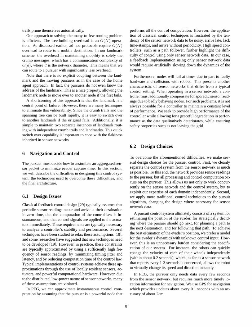
Figure 5: Spanning tree generated by PEG using 100mica2dot nodes. PEG uses a basic flooding algorithm thatadapts to different node densities and parent selection algo-rithms for better trees.

For the many-to-landmark routing, we first considered us-ing a simple grid-based routing such as [2] since location in-formation of each node is known and the network layout is agrid. However, we did not pursue this direction since it doesnot address link reliability issues, which is essential for cre-ating reliable routing over unreliable links. Our approach tothe many-to-landmark routing is based on a simple floodingmechanism that can rapidly build spanning trees with effi-cient routes and reasonable communication reliability. Thisapproach of rapid tree-building provides a quick fail over tocope with the flakiness found in sensor networks, and main-tains the soft-state design principle.

5.2 Building Good Trees

For many-to-landmark routing, we rely on a spanning treerooted at the landmark. All packets received or generated by anode are forwarded to its parent until they reach the landmark.

A common approach to building a spanning tree is to floodthe network with a beacon, and each node marks its parent inthe tree as the first node from which it receives the beacon,and then rebroadcasts the beacon. This approach of floodingthe network and routing using the reversed paths is used in ad-hoc routing algorithms such as AODV [23] and DSR [15] tobuild a topology quickly and trade off optimality for handlingmobility.

In such a topology formation process using flooding, twopotential problems must be addressed: quality route selec-tion and the broadcast storm problem [32]. The routing pro-tocol must avoid selecting bad links for routing; in partic-

6

ular, asymmetric connectivity should be avoided if routingpaths are formed by reversing the path discovered by flood-ing. Route selection solely using hop count cannot addressthese issues. The second issue is related to the broadcaststorm, which occurs when many nodes receive a beacon si-multaneously and attempt to rebroadcast the beacon immedi-ately. As a result, a storm of packet collisions is created andsignificant message losses would occur, which leads to an ill-formed topology containing manyback edges. Back edgesoccur when nodes miss a beacon message because of colli-sions, but later overhear it from nodes further down the tree.Back edges create unnecessarily long routes.

In exploring the different routing algorithms that use flood-ing for route discovery, not all of these issues are addressedby the protocols together. Empirical data in real sensor net-works have shown that if these issues are not addressed, theresulting topology will be ill-formed and the routing paths arelikely to be composed of long unreliable links not suitablefor multihop communication [12]. Following our simplicityguideline, we devised two simple mechanisms that interactwith the routing layer and the link layer to address these twoissues together.

Our first challenge in building spanning trees is route selec-tion. The goal is to ensure a high end-to-end packet transmis-sion rate while minimizing the tree’s depth. A node must con-sider both the quality of the link to its parent and its parent’stree depth. Without any rapid link estimation mechanism, werely on the received signal strength indicator (RSSI). Recentstudies for both sensor networks [39] and 802.11 networks[9] showed that RSSI is not a good predictor of link qual-ity. However, we can exploit spatial information to our ad-vantage to rely on RSSI values. With all nodes on roughlya grid configured to transmit at the same power and the factthat signal strength decays at least1/d2 when close to theground, it is possible to use RSSI threshold filter to scope theneighborhood relative to the physical distance. By determin-ing the link reliability of the nodes at different grid distancebeforehand, we can determine the RSSI values that maximizethe communication distance with good link bi-directional re-liability. This is essential for our landmark approach sinceit utilizes the reversed paths on the self-discovered spanningtree. We then establish a threshold RSSI value and only ac-cept messages that are above the threshold value. The rout-ing layer can be a simple algorithm that selects the short-est hop-count parent that passed the RSSI filter. Section 7presents measurements of the end-to-end reliability of therouting paths discovered by this approach.

The second challenge is to alleviate the broadcast stormproblem. We used a time-delayed back off that adapts to theobserved cell density. Broadcast storms occur because sev-eral nodes simultaneously attempt to rebroadcast the beacon.Suppose, instead, each node waits a random time before re-broadcasting the beacon, then network congestion decreases.With random back-off, the number of nodes in a radio cell

should be proportional to the number of potential wait times:as node density increases, nodes must wait longer periodsof time. Choosing the maximum wait time, then, requiresknowledge of the density; by choosing a sufficiently large in-terval, we can guarantee that each node has sufficient time tobroadcast its announcement without preventing other nodesfrom doing so.

An alternative extends the prior idea to result in a moreadaptive technique. Upon the reception of a broadcast mes-sage, each receiver starts a timer to fire in a random amountof time less thanR. Every time the node receives a broad-cast message before its timer expires, it resets the timer tofire in a new random time. Thus, theR interval from whichnodes wait is significantly smaller than in the naive protocolsince the total wait time is now adaptive and inversely pro-portional to the radio cell density, which is the number oftimes the same broadcast message is heard. In both sparseand dense networks, then, propagation within in local cellsfinish in R · n/2 time, wheren is the cell density andR ischosen uniformly.

One typical spanning tree is in Figure 5. The data wascollected from 100 mica2dot nodes with 2m spacing in eitherdirection. The landmark is located near the center of the field,at position (8,8). The tree has depth three, considerably lessthan if grid routing were used. Four nodes did not join thespanning tree because they are broken; Section 8 addressesbreakage. Additionally, most nodes’ parents are physicallycloser to the landmark. In those cases where this is not true,such as at (0,10), the physically closer parent is not any closerby the hop-count metric.

5.3 Efficient Landmark Routing

With the spanning tree built using the previous mechanism,any nodes in the network can send messages to the landmark,which must then be able to forward the messages to the mov-ing pursuers. To accomplish this, the pursuer periodically in-forms the network by picking a node in its proximity to routea special message to the landmark, thereby laying a “crumbtrail.” Instead of maintaining all the routing states at the land-mark, this message deposits a “crumb” with each interme-diate router on the spanning tree so that messages destinedto the pursuers at the landmark can reverse the path that thecrumb message took. Since each node along the crumb trailknows its next hop, communication overhead is smaller asit is not necessary to include the entire reverse path in eachpacket.

We support multiple concurrent crumb trails, allowing formany mobile destinations. Each crumb trail is identified bythe pursuer’s ID when it deposits its crumb.

The pursuer increments a sequence to give a time dimen-sion to these crumb trails such that these paths can dynami-cally track pursuer’s position. All such routing states are softin that they become stale over time, and thus, stale crumb

7

trails prune themselves automatically.Our approach to solving the many-to-few routing problem

is efficient. The tree-building overhead is anO(N) opera-tion. As discussed earlier, ad-hoc protocols requireO(N)overhead to route to a mobile destination. In our landmarkscheme, the overhead in maintaining mobility is solely thecrumb messages, which has a communication complexity ofO(d), whered is the network diameter. This means that wecan route to a pursuer with significantly less overhead.

Note that there is no explicit coupling between the land-mark and the moving pursuers as in the case of the homeagent approach. In fact, the pursuers do not even know theaddress of the landmark. This is a nice property, allowing thelandmark node to move over to another node if the first fails.

A shortcoming of this approach is that the landmark is acentral point of failure. However, there are many techniquesto eliminate this vulnerability. Since the crumb trails and thespanning tree can be built rapidly, it is easy to switch overto another landmark if the original fails. Additionally, it issimple to maintain two separate instances of landmark rout-ing with independent crumb trails and landmarks. This quickswitch over capability is important to cope with the flakinessinherited in sensor networks.

6 Navigation and Control

The pursuer must decide how to assimilate an aggregated sen-sor packet to minimize evader capture time. In this section,we will describe the difficulties in designing this control sys-tem, the techniques used to overcome these difficulties, andthe final architecture.

6.1 Design Issues

Classical feedback control design [29] typically assumes thatperiodic sensor readings occur and arrive at their destinationin zero time, that the computation of the control law is in-stantaneous, and that control signals are applied to the actua-tors immediately. These requirements are typically necessaryto analyze a controller’s stability and performance. Severaltechniques have been studied to relax these assumptions [18],and some researcher have suggested that new techniques needto be developed [19]. However, in practice, these constraintsare typically approximated by using a sufficiently high fre-quency of sensor readings, by minimizing timing jitter andlatency, and by reducing computation time of the control law.Typical implementations of control systems achieve these ap-proximations through the use of locally resident sensors, ac-tuators, and powerful computational hardware. However, dueto the distributed, low-power nature of sensor networks, manyof these assumptions are violated.

In PEG, we can approximate instantaneous control com-putation by assuming that the pursuer is a powerful node that

performs all the control computation. However, the applica-tion of classical control techniques is frustrated by the ten-dency of the sensor network data to be noisy, arrive late, lacktime-stamps, and arrive without periodicity. High speed con-trollers, such as a path follower, further highlight the diffi-culty of control using only sensor network data. In our case,a feedback implementation using only sensor network datawould require artificially slowing down the dynamics of thesystem.

Furthermore, nodes will fail at times due in part to faultyhardware and collisions with robots. This presents anothercharacteristic of sensor networks that differ from a typicalcontrol setting. When operating in a sensor network, a con-troller must additionally compensate for sporadic sensor read-ings due to badly behaving nodes. For such problems, it is notalways possible for a controller to maintain a constant levelof performance. We seek to provide high performance of thecontroller while allowing for a graceful degradation in perfor-mance as the data qualitatively deteriorates, while ensuringsafety properties such as not leaving the grid.

6.2 Design Choices

To overcome the aforementioned difficulties, we make sev-eral design choices for the pursuer control. First, we cleanlyseparate the control system from the sensor network as muchas possible. To this end, the network provides sensor readingsto the pursuer, but all processing and control computation oc-curs on the pursuer. This allows us not only to work concur-rently on the sensor network and the control system, but toexploit our expertise of each domain independently. Second,we apply more traditional control techniques to the pursuitalgorithm, changing the design where necessary for sensornetwork data.

A pursuit control system ultimately consists of a system forestimating the position of the evader, for strategically decid-ing where the pursuer should go next, for planning a path tothe next destination, and for following that path. To achievethe best estimation of the evader’s position, we prefer a modelfor the evader’s dynamics with unknown control input. How-ever, this is an unnecessary burden considering the specifi-cation of our system. For instance, the robots can quicklychange the velocity of each of their wheels independently(within about 0.2 seconds), which, as far as a sensor networkthat reports every 1-3 seconds is concerned, allows the robotto virtually change its speed and direction instantly.

In PEG, the pursuer only needs data every few secondsfrom the sensor network, but requires much more timely lo-cation information for navigation. We use GPS for navigationwhich provides updates about every 0.1 seconds with an ac-curacy of about 2cm.

8

Strategic Controller

Point Navigation Controller

Motor Controller

Coordinate Transformation

State Estimation

SensorNetwork

State Estimation

GPS

Filter

motors

High Speed

Dynamics

Low Speed Dynamics

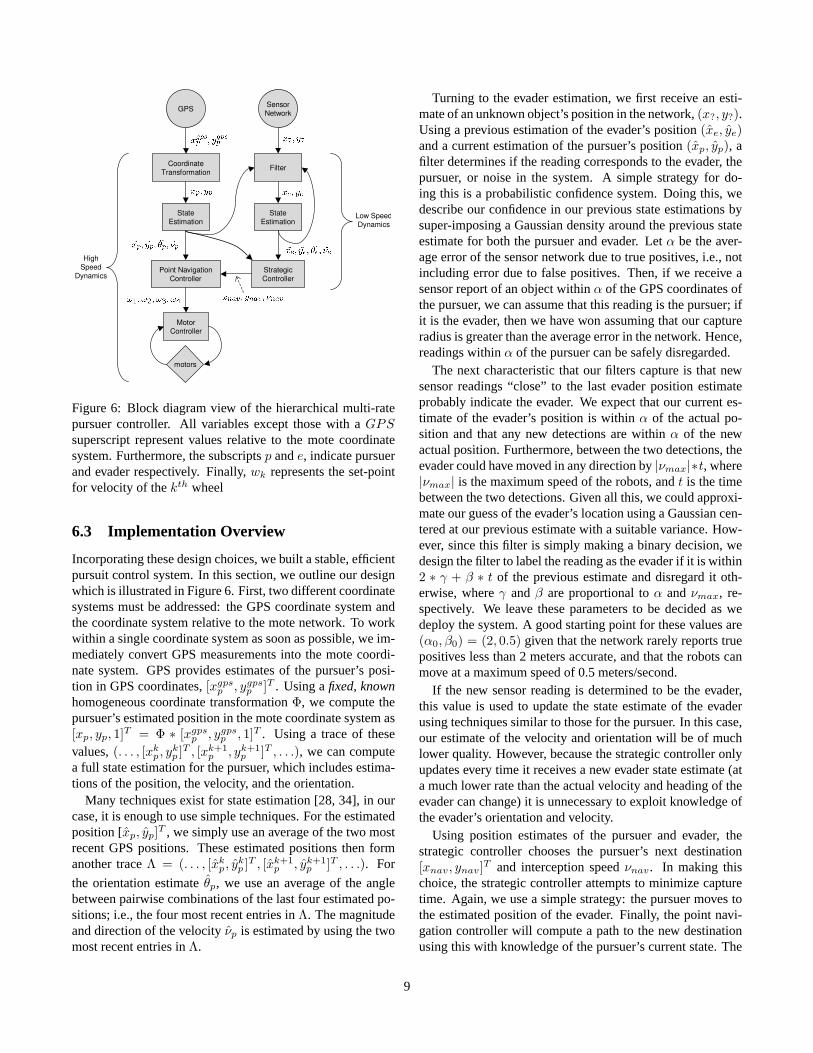
Figure 6: Block diagram view of the hierarchical multi-ratepursuer controller. All variables except those with aGPSsuperscript represent values relative to the mote coordinatesystem. Furthermore, the subscriptsp ande, indicate pursuerand evader respectively. Finally,wk represents the set-pointfor velocity of thekth wheel

6.3 Implementation Overview

Incorporating these design choices, we built a stable, efficientpursuit control system. In this section, we outline our designwhich is illustrated in Figure 6. First, two different coordinatesystems must be addressed: the GPS coordinate system andthe coordinate system relative to the mote network. To workwithin a single coordinate system as soon as possible, we im-mediately convert GPS measurements into the mote coordi-nate system. GPS provides estimates of the pursuer’s posi-tion in GPS coordinates,[xgps

p , ygpsp ]T . Using afixed, known

homogeneous coordinate transformationΦ, we compute thepursuer’s estimated position in the mote coordinate system as[xp, yp, 1]T = Φ ∗ [xgps

p , ygpsp , 1]T . Using a trace of these

values,(. . . , [xkp, yk

p ]T , [xk+1p , yk+1

p ]T , . . .), we can computea full state estimation for the pursuer, which includes estima-tions of the position, the velocity, and the orientation.

Many techniques exist for state estimation [28, 34], in ourcase, it is enough to use simple techniques. For the estimatedposition [xp, yp]T , we simply use an average of the two mostrecent GPS positions. These estimated positions then formanother traceΛ = (. . . , [xk

p, ykp ]T , [xk+1

p , yk+1p ]T , . . .). For

the orientation estimateθp, we use an average of the anglebetween pairwise combinations of the last four estimated po-sitions; i.e., the four most recent entries inΛ. The magnitudeand direction of the velocityνp is estimated by using the twomost recent entries inΛ.

Turning to the evader estimation, we first receive an esti-mate of an unknown object’s position in the network,(x?, y?).Using a previous estimation of the evader’s position(xe, ye)and a current estimation of the pursuer’s position(xp, yp), afilter determines if the reading corresponds to the evader, thepursuer, or noise in the system. A simple strategy for do-ing this is a probabilistic confidence system. Doing this, wedescribe our confidence in our previous state estimations bysuper-imposing a Gaussian density around the previous stateestimate for both the pursuer and evader. Letα be the aver-age error of the sensor network due to true positives, i.e., notincluding error due to false positives. Then, if we receive asensor report of an object withinα of the GPS coordinates ofthe pursuer, we can assume that this reading is the pursuer; ifit is the evader, then we have won assuming that our captureradius is greater than the average error in the network. Hence,readings withinα of the pursuer can be safely disregarded.

The next characteristic that our filters capture is that newsensor readings “close” to the last evader position estimateprobably indicate the evader. We expect that our current es-timate of the evader’s position is withinα of the actual po-sition and that any new detections are withinα of the newactual position. Furthermore, between the two detections, theevader could have moved in any direction by|νmax|∗t, where|νmax| is the maximum speed of the robots, andt is the timebetween the two detections. Given all this, we could approxi-mate our guess of the evader’s location using a Gaussian cen-tered at our previous estimate with a suitable variance. How-ever, since this filter is simply making a binary decision, wedesign the filter to label the reading as the evader if it is within2 ∗ γ + β ∗ t of the previous estimate and disregard it oth-erwise, whereγ andβ are proportional toα andνmax, re-spectively. We leave these parameters to be decided as wedeploy the system. A good starting point for these values are(α0, β0) = (2, 0.5) given that the network rarely reports truepositives less than 2 meters accurate, and that the robots canmove at a maximum speed of 0.5 meters/second.

If the new sensor reading is determined to be the evader,this value is used to update the state estimate of the evaderusing techniques similar to those for the pursuer. In this case,our estimate of the velocity and orientation will be of muchlower quality. However, because the strategic controller onlyupdates every time it receives a new evader state estimate (ata much lower rate than the actual velocity and heading of theevader can change) it is unnecessary to exploit knowledge ofthe evader’s orientation and velocity.

Using position estimates of the pursuer and evader, thestrategic controller chooses the pursuer’s next destination[xnav, ynav]T and interception speedνnav. In making thischoice, the strategic controller attempts to minimize capturetime. Again, we use a simple strategy: the pursuer moves tothe estimated position of the evader. Finally, the point navi-gation controller will compute a path to the new destinationusing this with knowledge of the pursuer’s current state. The

9

path we use is the one in which the pursuer moves forwardand turns toward its destination at the same time. Once theheading of the pursuer is in line with its destination, the pur-suer ceases turning and continues driving forward until itsdestination is reached. The point navigation controller real-izes the desired path by continually issuing new set points(ω1, ω2, ω3, ω4) for velocity of the robot wheels. The mo-tor controller then interfaces directly to the wheels to achievethese velocities.

In conjunction with the aforementioned processes, the con-troller maintains safety specifications by applying hard con-straints to the controller at various points. To ensure that thepursuer never leaves the network, the point navigation con-troller always compares the pursuer’s estimated state with thefixed, known values of the network boundary. If the pur-suer is leaving the network, the point navigation controllerdirects the pursuer to the center of the network until furthernotice. Additionally, if the strategic controller notices thatthe pursuer’s estimated state is within the capture radius ofthe evader’s estimated state, it has the point navigation con-troller stop the pursuer. The pursuer remains there until a newevader update farther away appears; at which time the controlsystem reinitiates pursuit of the evader.

7 Evaluation

7.1 Routing Service

One of the most important metrics for evaluating the multihoprouting service is end-to-end reliability, especially when thetopology is built over many unreliable links during a network-wide flooding. We created a set of micro-benchmark experi-ments to measure end-to-end success rate of packet deliveryof any random pair of nodes in the network using our land-mark routing. In all these measurements, we do not use linkretransmissions. For latency tests, there is no contention onthe channel because only one packet is being sent at a time.The end result is very promising. For paths that have lengthsvarying from 4 to 6 hops, the average of end-to-end successrate consistently falls in the range of 95% to 98%. This im-plies that our topology formation can build trees that are reli-able for bi-directional communication.

Another metric that is important to PEG is the end-to-endlatency in delivering the detection events to the moving pur-suers. As discussed before, our landmark routing approachtrades off route efficiency for simplicity and low protocoloverhead. The simplicity of the landmark routing schemeproduces routes that may be longer than necessary since themessage must pass through the landmark. For example, for aneighbor to route a message to an adjacent node, it must tra-verse through the landmark which could be far away. Therecould be delay from many sources: the time it takes a packetto travel, the processing time, MAC back off time, and rout-ing decision time. By observing the packet size and extra syn-

4 5 6 7 8 9 10 11 12150

200

250

300

350

400

450

500

550

600

650

Rou

te ti

me

(ms)

Number of hops

Figure 7: Latency of packets routed through PEG’s landmarkrouting algorithm. Each data point represents the averagetime to route 200 packets through the given number of hopson a 36 node indoor Mica 2.

chronization overhead coupled with the radio bandwidth, wecan conclude that a packet occupies the channel for 26.2 ms.The MAC waits a uniformly random time between 0.4 msand 13.0 ms before sending a packet, averaging in a 6.7 msdelay. We measured the latency that it takes for our algorithmto route packets in Figure 7 on a field of 36 sensor nodes. Fora least squares minimum fit on the data in the figure, we findthe slope of the line is 53 ms/hop, so we conclude processingtime is consistently around 20 ms. Even if the landmark routeis 6 hops while the optimal path is a single hop, the landmarkrouting will take 225 ms longer than necessary. In this time,the evader can only travel 13 cm, an insignificant distancecompared to the precision of the measurements. Thus, eventhough landmark routing may choose longer routes, the extrarouting time is within our requirements.

7.2 Tracking and Interception

To evaluate the system in a large scale demonstration on July14, 2003, we deployed a field of 100 nodes and performeda half-dozen runs1. The evader was controlled by a drivernot affiliated with PEG. The pursuer was able to success-fully capture the evader in all cases; we define success whenthe pursuer arrives within a grid square of the evader. Fig-ure 8 displays one such interception. Initially, the pursueris in a different orientation from the evader. It first orientsitself towards the evader before capturing the evader. The se-quence spans 26 seconds and ends when the pursuer touchesthe evader.

In order to display more quantitative data, we would liketo analyze network traces from an actual run from our July

1A movie of all runs is available athttp://webs.cs.berkeley.edu/nestdemo.mpg

10

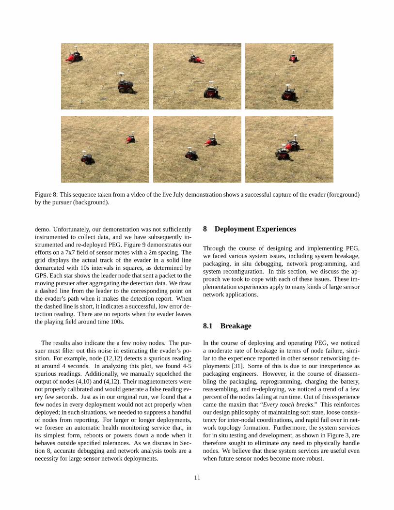
Figure 8: This sequence taken from a video of the live July demonstration shows a successful capture of the evader (foreground)by the pursuer (background).

demo. Unfortunately, our demonstration was not sufficientlyinstrumented to collect data, and we have subsequently in-strumented and re-deployed PEG. Figure 9 demonstrates ourefforts on a 7x7 field of sensor motes with a 2m spacing. Thegrid displays the actual track of the evader in a solid linedemarcated with 10s intervals in squares, as determined byGPS. Each star shows the leader node that sent a packet to themoving pursuer after aggregating the detection data. We drawa dashed line from the leader to the corresponding point onthe evader’s path when it makes the detection report. Whenthe dashed line is short, it indicates a successful, low error de-tection reading. There are no reports when the evader leavesthe playing field around time 100s.

The results also indicate the a few noisy nodes. The pur-suer must filter out this noise in estimating the evader’s po-sition. For example, node (12,12) detects a spurious readingat around 4 seconds. In analyzing this plot, we found 4-5spurious readings. Additionally, we manually squelched theoutput of nodes (4,10) and (4,12). Their magnetometers werenot properly calibrated and would generate a false reading ev-ery few seconds. Just as in our original run, we found that afew nodes in every deployment would not act properly whendeployed; in such situations, we needed to suppress a handfulof nodes from reporting. For larger or longer deployments,we foresee an automatic health monitoring service that, inits simplest form, reboots or powers down a node when itbehaves outside specified tolerances. As we discuss in Sec-tion 8, accurate debugging and network analysis tools are anecessity for large sensor network deployments.

8 Deployment Experiences

Through the course of designing and implementing PEG,we faced various system issues, including system breakage,packaging, in situ debugging, network programming, andsystem reconfiguration. In this section, we discuss the ap-proach we took to cope with each of these issues. These im-plementation experiences apply to many kinds of large sensornetwork applications.

8.1 Breakage

In the course of deploying and operating PEG, we noticeda moderate rate of breakage in terms of node failure, simi-lar to the experience reported in other sensor networking de-ployments [31]. Some of this is due to our inexperience aspackaging engineers. However, in the course of disassem-bling the packaging, reprogramming, charging the battery,reassembling, and re-deploying, we noticed a trend of a fewpercent of the nodes failing at run time. Out of this experiencecame the maxim that “Every touch breaks.” This reinforcesour design philosophy of maintaining soft state, loose consis-tency for inter-nodal coordinations, and rapid fail over in net-work topology formation. Furthermore, the system servicesfor in situ testing and development, as shown in Figure 3, aretherefore sought to eliminateany need to physically handlenodes. We believe that these system services are useful evenwhen future sensor nodes become more robust.

11

−2 0 2 4 6 8 10 12 14 16 18−2

0

2

4

6

8

10

12

14

(0,0) (2,0) (4,0) (6,0) (8,0) (10,0) (12,0)

(0,2) (2,2) (4,2) (6,2) (8,2) (10,2) (12,2)

(0,4) (2,4) (4,4) (6,4) (8,4) (10,4) (12,4)

(0,6) (2,6) (4,6) (6,6) (8,6) (10,6) (12,6)

(0,8) (2,8) (4,8) (6,8) (8,8) (10,8) (12,8)

(0,10) (2,10) (4,10) (6,10) (8,10) (10,10) (12,10)

(0,12) (2,12) (4,12) (6,12) (8,12) (10,12) (12,12)

0s

10s

20s 30s

40s

50s60s

70s

80s

90s

100s

110s

120s130s

140s

x physical position (meters)

y ph

ysic

al p

ositi

on (m

eter

s)

Figure 9: Intruder tracking using PEG. Evader GPS positionis shown as a solid line. Detection event leaders are shownas stars. Using dotted lines, leaders are linked to the evader’sposition at the time of detection.

8.2 Packaging

A real-world sensor deployment must carefully consider nodepackaging, and we discovered that that packaging require-ments for deployment are different from those for develop-ment. For development, the packaging should expose ac-cess for convenient debugging, reprogramming, and batteryrecharging. However, we did not properly anticipate suchneed, and during development, we would frequently need todisassemble the packaging in order to fix broken components,reprogram the nodes, or recharge the batteries. If we had bet-ter foresight in our design, we would have designed the pack-aging to support reprogramming and recharging without fullpackage disassembly.

After deployment we discovered that the packaging wasinterfering with the magnetometer. The piano wire antenna,battery, and metallic spring base all align the magnetic fieldin the proximity of the magnetometer, significantly reducingits sensitivity and overall range of detection. The design pro-cess should accommodate a series of revisions, because de-fects may only become apparent when the complete design isimplemented and deployed in the sensing environment.

8.3 Debugging

Debugging large sensor network applications at deploymenttime is a challenging experience. Pre-deployment testing us-ing simulations and controlled experiments over testbeds areextremely useful as they allow us to extract information aboutthe external and internal states of each node. However, in a

real deployment, collecting state information can be difficult,especially when the packaging is designed for deployment.For example, even if the EEPROM fully logs the transient in-ternal states of each node, correlating them in a network-widetemporal order can be difficult, especially without time syn-chronization. In our deployment, we did not have adequatetime to explore this option.

Instead, we exploit a large antenna to snoop on networktraffic. This non-intrusive approach allows the collection ofas much external states of the network as possible, does notaffect the application, and enables a direct communicationwith each of the node in the network.

A set of services under the node management category inFigure 3 are implemented to address in situ debugging. Addi-tionally, we place a version control number into each binaryto ensure code compatibility across all the nodes in the net-work. We use a basic “ping” like service to verify that a nodeis up. The ping reply also reports the version control numberof its code binary, allowing us to detect incompatible bina-ries. In addition, some of the basic primitives for node man-agement such as node reset, sleep, and active mode controlare also supported over wireless control.

The big antenna allows us to remotely control and debugeach node in the network. We implement a set of managementscripts on a PC computer to invoke the sensor node manage-ment services to administrate the system through the antenna.Packet traces are archived for off-line debugging and visual-ization of the entire system to understand the global behavior,which is extremely useful in system tunings. Nodes can sendpackets with an ASCII text payload to act as a “printf” tosignal the occurrence of some critical debugging events in ahuman readable form.

8.4 Hierarchy of Programming and Reconfig-uration

In sensor networks, the need for a form ofin situ program-ming presents a new kind requirement for remote configura-tion tools. Besides the common need for wireless network-wide reprogramming, there is also a need to perform in situprotocol parameter tuning since analytical analysis is ofteninsufficient to accommodate environmental effects. For ex-ample, there are configuration options of the code that needto be decided at the time of deployment, including the appli-cation’s sensing policy, sensor calibrations, and communica-tions parameters that rely on the cell density. Furthermore,some of these configurations may need to be set on varyinggranularities, ranging from individual nodes, a select few sub-set of nodes, to the entire set of nodes en masse. We have im-plemented both the network reprogramming and config ser-vices as shown in Figure 3 to address these needs.

Our design supports wireless network programming, whichis an alternative solution to installing new binaries over manynodes by hand. For a team of five people working with one

12

hundred nodes, manual programming takes two hours with anadditional two hours to re-deploy the nodes in the field. Thisapproach is clearly not amenable to a rapid debug and testcycle.

Using network programming, nodes receive the binary im-age over the radio. By exploiting the shared wireless medium,many nodes can be reprogrammed simultaneously and selec-tively. We anticipated using network reprogramming for ourdeployment, but we could not develop a sufficiently reliablenetwork reprogramming mechanism for our purposes2. Giventhe problems we encountered at the time, the entire processwould have taken longer than individually reprogrammingeach node.

Interestingly, with a network service we call Config, thelimitations of manually programming each node and our in-ability use network reprogramming did not pose a great hin-drance in our deployment. We spend the majority of our timetuning the algorithms to work properly at scale in the envi-ronment. The Config service addresses this issue efficientlyand allows run-time adjustments of the internal states of eachnode. For example, Config allows us to selectively enablesections of the code, adjust parameters, modify calibrationvalues, and adjust variables at run time.

Config is a smart configuration system that takes the placeof a traditional approach to using a local configuration fileper node. Configuration values are declared in the code witha specific configuration identifier, as shown in this example:

//!! Config 31 {uint16_t RFThreshold = 200;}

In this case, the RFThreshold parameter, with a defaultvalue of 200, is preprocessed with compilation tools to con-vert it to be a member in a global Config data structure. Con-fig is tightly integrated with the scripting environment in Mat-lab, allowing the large antenna to be used for debugging.Therefore, it is easy to change configuration values for a sub-set of the nodes or all the nodes from a PC in run time.

When a user changes a node’s configuration value, thechange is automatically reflected in that node’s global Con-fig data structure. And, the application is notified throughan asynchronous event of the change to the data value. Con-fig also supports queries of the current set of configurationvalues on each node. With a rich configuration capability inplace and a bit of creative programming to utilize it, the re-sulting application is quite malleable, saving us a lot of timefrom installing new code images.

9 Conclusion

Designing and implementing PEG enables us to establish rel-evant system design principles that are useful to other sensornetworking systems. Our whole-system design analysis pro-vides a clean process of problem decomposition. It allows

2Subsequent work has improved upon our initial foray. [27]

complexity to be placed at the appropriate levels of the sys-tem to achieve overall simplicity in system implementation.Simplicity is further achieved by exploiting environmentaland physical characteristics of the application at deploymenttime. Protocols should exploit soft state, loose consistency,and rapid fail over when appropriate to cope with the lossywireless channel and the somewhat unreliable sensor networkhardware platform. The system management and debugginginfrastructure should be well designed to anticipate the needof system reconfigurations at deployment time.

Our system decomposition allows each of the subsystemsto be reusable by a wide variety of sensor network appli-cations. The neighborhood abstraction and leader electionmechanisms apply to any monitoring system requiring localdata aggregation. The density adaptive flooding mechanismavoids the broadcast storm problem for other data dissemina-tion protocols. The landmark routing subsystem is useful forany application with moving entities. The network manage-ment and debugging services are useful for deploying othersensor networks. The data filter and robustness of the controlsystem design are applicable to other sensor network applica-tions with embedded actuators.

We demonstrate a working system that not only monitorssensory data but also tracks and controls a higher tier systemto accomplish a cooperative task in real time. The systemassumes very little processing and communication require-ments on the sensor tier. Furthermore, throughout our designwe exploit the physical properties of PEG to achieve a func-tional, simple design that is robust to failures. We believe thesame design philosophy should be followed in building futuresensing and actuating systems.

Acknowledgments

We’d like to thank everyone who worked on PEG, includ-ing: Phoebus Chen, Fred Jiang, Jaein Jong, Sukun Kim, PhilLevis, Neil Patel, Joe Polastre, Robert Szewczyk, TerrenceTong, Rob von Behren, and Kamin Whitehouse. This work isfunded in part by the DARPA NEST contract F33615-01-C-1895 and Intel Research.

References

[1] Anonymous. InCitation omitted for blind reviewing; we will make thisavailable to any of the program chairs at the reviewer’s request.

[2] A. Arora, P. Dutta, S. Bapat, V. Kulathumani, H. Zhang, V. Naik,V. Mittal, H. Cao, M. Gouda, Y. Choi, T. Herman, S. Kularni, U. Aru-mugam, M. Nesterenko, A. Vora, and M. Miyashita. Line in the sand:A wireless sensor network for target detection, classification, and track-ing. In OSU-CISRC-12/03-TR71, 2003.

[3] Javed Aslam, Zack Butler, Florin Constantin, Valentino Crespi, GeorgeCybenko, and Daniela Rus. Tracking a moving object with a binarysensor network. InProceedings of the first international conferenceon Embedded networked sensor systems, pages 150–161. ACM Press,2003.

13

[4] Ken Birman. The process group approach to reliable distributed com-puting. In Communiation of the ACM, volume 36(12), pages 37–53,1993.

[5] B. Blum, P. Nagaraddi, A. Wood, T. Abdelzaher, S. Son, andJ. Stankovic. An entity maintenance and connection service for sen-sor networks, 2003.

[6] Richard R. Brooks and Parameswaran Ramanthan. Distributed targetclassification and tracking in sensor networks. InIn Proceedings of theIEEE, pages 1163–1171, August 2003.

[7] Alberto Cerpa, Jeremy Elson, Deborah Estrin, Lewis Girod, MichaelHamilton, and Jerry Zhao. Habitat monitoring: Application driver forwireless communications technology. InACM SIGCOMM Workshopon Data Communications in Latin America and the Caribbean, April2001.

[8] David Cheriton. Understanding the limitations of causally and totallyordered communication. InSOSP. ACM, December 1993.

[9] Douglas S. J. De Couto, Daniel Aguayo, John Bicket, and Robert Mor-ris. A high-throughput path metric for multi-hop wireless routing. InProceedings of the 9th annual international conference on Mobile com-puting and networking, pages 134–146. ACM Press, 2003.

[10] Deborah Estrin, Lewis Girod, Greg Pottie, and Mani Srivastava. In-strumenting the world with wireless sensor networks. InInternationalConference on Acoustics, Speech, and Signal Processing (ICASSP2001), 2001.

[11] Qing Fang, Jie Li, Leonidas Guiba, and Feng Zha. Roamhba: main-taining group connectivity in sensor networks. InProceedings of thethird international symposium on Information processing in sensor net-works, pages 151–160. ACM Press, 2004.

[12] Deepak Ganesan, Bhaskar Krishnamachari, Alec Woo, David Culler,Deborah Estrin, and Stephen Wicker. Complex behavior at scale: Anexperimental study of low-power wireless sensor networks. InTechni-cal Report UCLA/CSD-TR 02-0013, February 2002.

[13] J.P. Hespanha and Maria Prandini. Optimal pursuit under partial infor-mation. InIn Proceedings of the 10th Mediterranean Conference onControl and Automation, July 2002.

[14] Jason Hill, Robert Szewczyk, Alec Woo, Seth Hollar, David Culler, andKristofer Pister. System architecture directions for networked sensors.In Proceedings of ACM ASPLOS IX, pages 93–104, November 2000.

[15] D. Johnson and D. Maltz. Dynamic source routing in ad hoc wirelessnetworks. InMobile Computing, pages 153–181. Kluwer AcademicPublishers, 1996.

[16] Juan Liu, Jie Liu, James Reich, Patrick Cheung, and Feng Zhao. Dis-tributed group management for track initiation and maintenance in tar-get localization applications. InIn Proceedings of the 2nd Workshopon Information Processing in Sensor Networks (IPSN ’03), April 2003.

[17] Samuel Madden.The Design and Evaluation of a Query ProcessingArchitecture for Sensor Networks. PhD thesis, UC Berkeley, 2003.

[18] Pau Marti, Gerhard Fohler, Krithi Ramamritham, , and Josep M.Fuertes. Jitter compensation for real-time control systems. In22ndIEEE Real-Time Systems Symposium, London, December 2001.

[19] Pau Marti, Ricard Villa, Josep M. Fuertes, and Gerhard Fohler. Stabil-ity of on-line compensated real-time scheduled control tasks. InIFACConference on New Technologies for Computer Control, Hong Kong,November 2001.

[20] V. Park and M.S. Corson. A highly adaptive distributed routing algo-rithm for mobile wireless networks. InIn Proceedings of the IEEEINFOCOM ’97, April 1997.

[21] T.D. Parsons. Pursuit-evasion in a graph. InTheory and Application ofGraphs (Y. Alani and D.R. Lick, eds., pages 426–441. Springer-Verlag,1976.

[22] Hanna Pasula, Stuart Russel, Michael Ostland, and Ya’acov Ritov.Tracking many objects with many sensors. InIn Proceedings of IJCAI-99, 1999.

[23] Charles E. Perkins and Elizabeth M. Royer. Ad hoc on-demanddistance-vector (aodv) routing. InProceedings of the 2nd IEEE Work-shop on Mobile Computing Systems and Applications, 1999.

[24] Charles E. Perkins, Bobby Woolf, and Sherman R. Alpert. Mobile ipdesign principles and practices, January 1998.

[25] Gregory Pottie and William Kaiser. Wireless integrated network sen-sors. InCommunications of the ACM, May 2000.

[26] D.B. Reid. An algorithm for tracking multiple targets. InIEEE Trans-actions on Automatic Control, volume 24:6, 1979.

[27] Niels Reijers and Koen Langendoen. Efficient code distribution inwireless sensor networks. InProceedings of the 2nd ACM interna-tional conference on Wireless sensor networks and applications, pages60–67. ACM Press, 2003.

[28] Branko Ristic, Sanjeev Arulampalam, and Neil Gordon.Beyond theKalman Filter: Particle Filters for Tracking Applications. ArtechHouse, February 2004.

[29] Wilson J. Rugh.Linear System Theory. Information and System Sci-ences Series. Prentice Hall, Upper Saddle River, New Jersey 07458,second edition, 1996.

[30] I. Suzuki and M. Yamashita. Searching for a mobile intruder in a polyg-onal region. InSIAM J. Comput., volume 21, pages 863–888, October1992.

[31] Robert Szewczyk, Joseph Polastre, Alan Mainwaring, and DavidCuller. Lessons from a sensor netowkr expedition. InIn the 1st Eu-ropean Workshop on Wireless Sensor Networks (EWSN 04), January2004.

[32] Yu-Chee Tseng, Sze-Yao Ni, Yuh-Shyan Chen, and Jang-Ping Sheu.The broadcast storm problem in a mobile ad hoc network.Wirel. Netw.,8(2/3):153–167, 2002.

[33] P.F. Tsuchiya. The landmark hierarchy, a new hierarchy for routing invery large networks. InSpecial Interest Group on Data Communication(SIGCOMM), pages 36–42, 1988.

[34] Pravin Varaiya and P.R. Kumar.Stochastic Systems: Estimation, Iden-tification, and Adaptive Control. Information and System Sciences Se-ries. Prentice Hall, Upper Saddle River, New Jersey 07458, 1986.

[35] R. Vidal and S. Sastry. Vision-based detection of autonomous vehi-cles for pursuit-evasion games. InIFAC World Congress on AutomaticControl, 2002.

[36] Matt Welsh and Geoff Mainland. Programming sensor networks usingabstract regions. InIn Proceedings of the First USENIX/ACM Sympo-sium on Networked Systems Design and Implementation (NSDI’ 04),March 2004.

[37] Kamin Whitehouse, Cory Sharp, Eric Brewer, and David Culler. Hood:a neighborhood abstraction for sensor networks. InIn Proceedings ofACM International Conference on Mobile Systems, Applications, andServices (MobiSys ’04). ACM Press, June 2004.

[38] Feng Zhao, Jie Liu, Juan Liu, Leonidas Guibas, and James Reich. Col-laborative signal and information processing: An information directedapproach. InProceedings of the IEEE, pages 91(8):1999–1209, 2003.

[39] Jerry Zhao and Ramesh Govindan. Understanding Packet Delivery Per-formance in Dense Wireless Sensor Networks. InProceedings of thefirst international conference on Embedded networked sensor systems,pages 1–13. ACM Press, 2003.

14