Design and Implementation of a Pillbox Antenna for an AirborneImaging Radar

S.B. Gambahaya, M.R. InggsRadar Remote Sensing Group, Department of Electrical Engineering

University of Cape Town, Private Bag, Rondebosch 7701, South AfricaEmail: mikings@ebe.uct.ac.za Web: http://www.rrsg.uct.ac.za

Tel: +27 21 650 2799 Fax: +27 21 650 3465

June 23, 2006

Abstract

This paper describes the design and implementationof the fan beam radar antenna for SASAR II. TheSASAR II project is an ongoing initiative to demon-strate the capability of South Africa to produce highquality imagery using (SAR) Synthetic Aperture Radartechniques. The Radar Remote Sensing Group (RRSG)at UCT was commissioned by Denel Aviation Systems,SunSpace, and UCT to design, implement and test ahigh resolution X-band SAR, as a follow-on to the suc-cessful VHF Radar developed and flown in 2000. Theantenna was to be able to radiate through a cabin win-dow of an Aerocommander aicraft. The antenna speci-fications were determined from image signal process-ing requirements [12]. The pillbox was chosen dueto its relative simplicity in design and analysis. MAT-LAB simulations were carried out to predict the radia-tion characteristics of the antenna. The fully fabricatedantenna was then tested and comparisons were madebetween the actual performance of the antenna and the-oretical predictions. This paper has been written as atutorial, and contains some detailed information of test-ing using relatively primitive antenna test facilities.

1 Introduction

A pillbox antenna is a linearly polarized cylindrical re-flector embedded between two parallel plates. It is usu-ally fed by a waveguide [9] [19]. The pillbox is partof a family of antennas called fan beam antennas whichproduce a wide beam in one plane and a narrow beam

in the other [15] [19].The pillbox antenna can be dual-polarized and is also a relatively wide bandwidth an-tenna. The pillbox antenna has existed for at least fiftyyears and it was used for military surveillance radarsduring the Second World War and just after the Sec-ond World War [19]. The British version was calledthe cheese antenna. The primary difference between thecheese antenna and the pillbox is the separation of theparallel plates and their possible modes of electromag-netic propagation [9] [19]. The following requirementswere specified for the radar antenna of the SAR systemby the system engineer [10] [11] [12].

Figure 1: Pillbox or Cheese Antenna (from [19]).

1. A pillbox antenna with a single mode of propaga-tion is to be designed, implemented and tested tomeet specifications. If several modes can propa-gate simultaneously, there is no control over whichmode actually contains the transmitted signal, thuscausing dispersions, distortions and erratic opera-

1

tion [16].

2. The operating centre frequency is set tof◦ = 9.3GHz.

3. The antenna operating bandwidth which is deter-mined by the transmitter isB = 100 MHz.

4. The antenna 3 dB azimuth beamwidth shall be3.8◦

and the elevation beamwidth shall be25◦.

5. The peak power that the antenna system can han-dle is 3.5 kW.

6. The antenna should be able to operate at a plat-form height of 3000-8000 m. The aircraft cabinis pressurised at the equivalent of 8000 feet. Theantenna shall be mounted inside the aircraft, press-ing against the perspex window, to avoid costly air-frame modifications.

The advantages of using a pillbox antenna for radar ap-plications are given below [19]

• It is easy to design and the cost of production islow.

• It is dually-polarized and it is also a wide band an-tenna.

• It has a high power handling capability.

2 Design of Antenna

2.1 Design Theory

The pillbox design was based on the aperture fieldmethod as well as diffraction theory of aperture anten-nas. By using geometrical optics [6] and the diffrac-tion theory of antennas we can predict the far-field ofan antenna. There is a Fourier Transform relationshipbetween the far-field and the aperture field which isanalogous to the relationship between Fourier spectraand time domain waveforms (even though waveformsare one-dimensional). The far-field can be predicted bytaking the Fourier Transform of the tangential compo-nent of the E-field. This one dimensional treatment isadequate for discussing the pillbox antenna since its di-rectivity can be separable into a product of directivitiesof one-dimensional apertures made up of the length andwidth of the aperture [3]. Once the aperture fields arehave been calculated, we use equation 1 to predict the

far-field pattern of the antenna in the E and H-planes [5][6][7]:

E (θ) =

∫ x/2

−x/2

f (x) ejkx sin θdx (1)

Wheref (x) is the aperture field distribution function across theaperture, ‘x’ is the length of the aperture and ‘k’ is thewavenumber.

2.2 Offset fed Pillbox Design

Offset prime-focus-reflectors are desirable because ofthe ability to offset the feed enough so that it is notin the way of the aperture to cause aperture blockagewhich consequently raises the sidelobe levels. How-ever, offset-fed reflectors with a linearly polarized feedsuffer from higher cross-polarization than axisymmet-ric reflectors [20]. Here the major design emphasis is onthe choice of offset angle or feed pointing angleψf toreducing sidelobe levels and also reduce cross polariza-tion without a sacrifice in gain [20].

Offset reflector antennas inherently produce off-axiscross-polarization in the principal plane normal to theoffset plane. The cross-polarization is a result of theasymmetric mapping of the otherwise symmetrical pat-tern into the aperture antenna [2] [18]. We wish to keepthe cross-polarization levels to at least 30 dB belowthe peak of the co-polar pattern for satisfactory perfor-mance of the antenna [15][18].

2.2.1 The Geometry

The geometry of the offset fed configuration is shownin figure 2. The primary parameters that we can controlare the degree of offset by varyingh and the aiming ofthe feed antenna(the angleψ) . In this paper we con-sider the case of the more than fully offset feed,h > 0to provide a blockage-free region for the structures inthe focal region. In practice in order to keep spill-overlosses reasonable the feed is aimed within the range [19][20]:

40◦ ≤ ψf ≤ 60◦

The definitions of the symbols used in Figure 2 aregiven below where

Figure 2: Offset Parabolic Reflector Geometry (from[20])

D = Diameter of the projected apertureof the cylindrical reflector

h = Offset distanceDp = Diameter of the projected aperture

of the parent paraboloid.F = Focal length.f/Dp = ‘f/D′ of parent reflector.ψf = Angle of antenna pattern peak rela-

tive to reflector axis of symmetryψc = Value ofψf when the feed is aimed

at the aperture centre.ψE Value ofψf when the feed yields an

equal edge illumination .ψf = Value ofψf which bisects the reflec-

tor subtended angle.FT = Feed edge taper;FT ≥ 0.EI = Edge illumination;EI = −(FT +

SPL); SL is the spherical spreadloss.

The spherical spread loss of the antenna is given by[20] :

SPL (ψ) = −20 log

[

cos2ψ

2

]

(2)

Quoting ’W. Stutzman’, several numerical sim-ulations using the physical optics computer codeGRASP−7 on reflector antennas yielded the followingresults [20]:

• “ Several numerical simulations showed that theorientation of the feed strongly influences cross-polarization. In particular small feed pointing an-gles lead to high spillover which would raise the

sidelobe and cross-polarization levels for a highgains.

• Large f/Dpvalues which lead to reduced feedpointing anglesψf cause degradation in sidelobelevels even though the cross-polarization level im-proves. Based on the above observations, wecan thus try to optimize the feed pointing or off-set angle to yield the lowest sidelobes and cross-polarization levels with the smallest penalties ingain. A feed pointing angle ofψf = ψE achievesthis specification and it also turns out that this op-erating point produces a balanced aperture illumi-nation, that is the edge illumination levels (in theplane of offset) in the aperture are equal ”.

The diameter of the parent parabola was fixed atDp =126 cm and curvature of the reflector wasf/Dp = 0.3to achieve a good compromise between sidelobe levelsand cross-polarization. The design presented here wasa single polarisation version, to simplify the feed horndesign.

2.2.2 Reflector Aperture Dimensions

We calculated the anglesψL andψU which are the an-gles subtended by the lower and upper edges of the re-flector respectively using equation 3 [2][16] [19] :

ρ (ψ) = 2f tan

(

ψ

2

)

(3)

• The angle subtended by the upper edge of the re-flector is calculated as follows:

ψU = 2· arctan

(

64

2 × 38

)

≈ 80◦

• The angle subtended by the lower edge of the re-flector is calculated as follows:

ψL = 2 · arctan

(

7

2 × 38

)

≈ 11◦

Whereρ is the perpendicular distance from the par-ent reflector centre to the upper edge. The feed pointing

angle wasψB = 45◦. A simple MATHCAD calcula-tion gave the length of the feed horn in the offset planeto achieve an equal edge illumination of approximately-10 dB at the edges. The length of the horn was cal-culated to be 6.5 cm. It was only later discovered thatthere was an error in the initial calculation of the hornazimuth dimension, it should have been 6 cm instead.

• The additional taper due to the space loss inψL

is small and can be neglected. The SL atψU iscalculated as follows:

SPLU = −20 log

[

cos2(

80

2

)]

= 4.5 [dB] (4)

The space loss will introduce an additional 4.5 dBtaper in the secondary aperture field distribution at theupper edge of the reflector.

• The lengthDaz of the aperture required to pro-duce an edge illumination of -10 dB at the reflectoredges is calculated by the following equation [16][19]:

Daz = (1.05Aedge + 55.95)λ

θaz

= ((1.05◦ × 10) + 55.95)3.2

3.8

= 56 [cm] (5)

• The width of the aperture for a uniform illumina-tion in the elevation plane is calculated by the fol-lowing equation:

Del =57λ

θel

=57 × 3.2

25

= 7 [cm] (6)

• The offset distance was set toh = D/8 so that’h = 7 cm’.

2.2.3 Directivity of Pillbox Antenna

GD ≈1

k·

4π

θaz · θele

=4π

0.44 × 0.066× 1.12

= 25.6 [dBi] (7)

whereθazandθele are the principal azimuth and ele-vation beamwidths respectively, ‘k’ is the beam broad-ening factor relative to a uniform distribution, which isalso the loss in directivity. The value ofk=0.44 was ap-proximated from the taper imposed on the upper edge ofthe parabolic reflector relative to a uniform distribution.The gain of an antenna which includes the directivityand power gain are well documented in [1].

2.2.4 Aperture Field Method:Predicted AzimuthPattern

We used the aperture field method to determine the off-set reflector pattern in the azimuth plane atψf = 45◦.We evaluated the equivalent Huygens sources at theaperture and integrated these sources to obtain the re-flector far-field pattern[2][9] [14]. This section showsthe steps taken to predict the reflector far-field.

The equation of the parabolic cylinder in polar coor-dinates is given as [6]:

ρ (ψ) =f

cos2 (ψ/2)(8)

=2f

1 + cosψ

The primary and secondary power flows are equaland given as [6]:

P (y) = I (ψ) dy (9)

whereIaz (ψ) is the feed far-field power pattern ofthe horn in units of watts per radian-meter.P (y) is thesecondary power flow in units of watts per radian-meter.

The feed radiation pattern in the H-plane is modelledby the following Fourier Transform expression at thefeed pointing angleψf = 45◦ [9]:

Eaz (ψ − ψoffset) =

∫ a1/2

−a1/2

E0 cos(πx

a

)

ejαdx

where

α =2π

λx sin

(

ψ − ψoffset)

(10)

The azimuthal power pattern of the horn is given by:

Iaz (ψ) = I2az (ψ − ψoffset) (11)

The equation relating the primary and secondarypower distributions is given by the following expression[6]:

P (y) =I (ψ)

ρ (ψ)(12)

=Iaz (ψ) cos2 (ψ/2)

f

The aperture field of the reflector is given by the fol-lowing expression [6]:

faz (y) = P [(y)]1/2 (13)

The far-field pattern of the reflector is then given bythe following Fourier Transform expression [6]:

Faz (ψ) =

∫ Daz/2

−Daz/2

faz (y) ej2π

λy sinψdy (14)

Whereh = Offset distance = distance from the axisof symmetry(ies) to the lower reflector edge.Daz/2 ishalf the span of the parent parabola.

2.2.5 Predicted Elevation Pattern

Assumingthe tangent plane approximation of phys-ical optics [5], we can predict the elevation pattern bythe following expression:

Eel (ψ) =

∫ Del/2

−Del/2

E◦ej 2π

λy sinψdy (15)

WhereDel/2 ≤ h ≤ −Del/2 is the height of thepillbox aperture.

The power radiation pattern in the vertical plane isgiven by [9] :

Pel (θ) = E2el (θ) (16)

2.3 Design of Feed Horn

A pyramidal horn can only be constructed for dimen-sions that satisfy the following equation [2] [13]:

(a1 − a)2

[

(

ρh

a1

)2

−1

4

]

= (17)

(b1 − b)2

[(

ρe

b1

)

−1

4

2]

The dimension of the horn to achieve a -10 dB edgeillumination in the azimuth planes was calculated inMATHCAD and found to bea1 = 6.0 cm. TheTE1,0

waveguide dimension a= 2.286 cm. In the elevationplane the horn dimensionb1 is determined by the sep-aration of the plates, thereforeb1 = 7 cm. The TE1,0

waveguide dimensionb = 1.016 cm.

• We chose a flare angle of20◦ in the E-plane andusing simple trigonometry, the slant length in theE-plane is calculated as follows:

• By making use of equation 17 and makingρh thesubject of the formula, the slant length in the H-plane is calculated as follows:

(a1 − a)2[

(

ρh

a1

)2

−1

4

]

= (b1 − b)2[

(

ρeb1

)2

−1

4

]

( ρh

6.5

)2

≈ 4.055

ρh = 13.09 [cm] (18)

• From simple trigonometry,ρh = 13.09 cm corre-sponds to an H-plane flare angle calculated as:

ψh = arcsin

(

3.25

13.09

)

ψh = 14.5◦ (19)

2.4 Antenna Construction

Figure 3: Top View of Fully Constructed Antenna

Figure 4: Front View of Fully Constructed Antenna

The feed horn was made out of brass of 1 mm thicknessand the parallel plates as well as the cylindrical reflec-tor were made out of 2mm thick aluminium. The keyaspects in the manufacturing of the antenna prototypeare listed below:

• The plates had to be flat with no bending as thismight excite modes other than TEM.

• The feed positioning is important and in this re-gard it was designed so that it was embedded be-tween the parallel plates and made movable backand forth so as to locate the phase centre. Plasticscrews were used to fasten the feed in place.

• We avoided vertical walls on either side of the pill-box as these might cause internal reflections andaffect performance as well as possibly short out theE field and cause propagation of higher modes. In-stead we used PVC dielectric posts to support theparallel plates and maintain rigidity.

• Any gaps between the plates and the reflector wereavoided as this would cause radiation leakage andthis might affect the far-field pattern and gain mea-surements. However we assumed that tiny gaps

created by bending the reflector should not affectour readings significantly.

3 Results

3.1 Return Loss

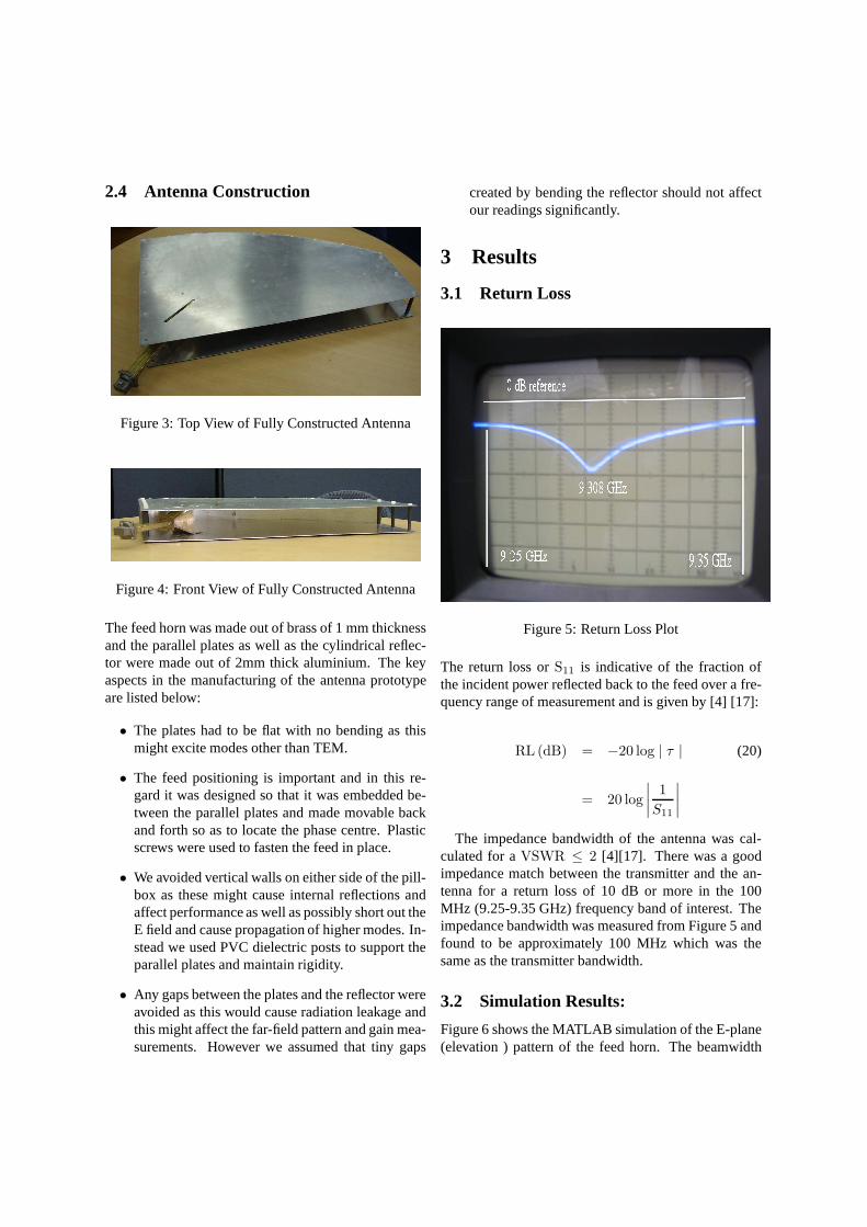
Figure 5: Return Loss Plot

The return loss orS11 is indicative of the fraction ofthe incident power reflected back to the feed over a fre-quency range of measurement and is given by [4] [17]:

RL (dB) = −20 log | τ | (20)

= 20 log

∣

∣

∣

∣

1

S11

∣

∣

∣

∣

The impedance bandwidth of the antenna was cal-culated for aVSWR ≤ 2 [4][17]. There was a goodimpedance match between the transmitter and the an-tenna for a return loss of 10 dB or more in the 100MHz (9.25-9.35 GHz) frequency band of interest. Theimpedance bandwidth was measured from Figure 5 andfound to be approximately 100 MHz which was thesame as the transmitter bandwidth.

3.2 Simulation Results:

Figure 6 shows the MATLAB simulation of the E-plane(elevation ) pattern of the feed horn. The beamwidth

was found to be approximately25◦. The first sidelobeswere at a level of -13 dB.

−100 −80 −60 −40 −20 0 20 40 60 80 100−70

−60

−50

−40

−30

−20

−10

0

theta−d,degrees

radi

atio

n in

tens

ity,d

Bi

Far field elevation pattern

−3 dB

−25 degrees

Figure 6: E-plane Feed Horn Pattern

Figure 7 shows the H plane pattern (azimuth pattern)of the feed horn at a feed pointing angle of45◦. The 3dB beamwidth is approximately37◦. The largest side-lobes were at a level of approximately -21 dB.

−100 −80 −60 −40 −20 0 20 40 60 80 100−70

−60

−50

−40

−30

−20

−10

0

radi

atio

n in

tens

ity d

Bi

H plane offset feed pattern

theta−d, degrees

37 degrees

− 3dB

Figure 7: H-plane Pattern of Feed Horn (offset feed)

Figure 8 shows the MATLAB simulation of the pre-dicted azimuth pattern of the pillbox antenna. The H-plane beamwidth was found to be approximately3.8◦

and the first time sidelobes were found to be at a levelof -23 dB.

−20 −15 −10 −5 0 5 10 15 20

−55

−50

−45

−40

−35

−30

−25

−20

−15

−10

−5

theta−d,degrees

radi

atio

n in

tens

ity,d

Bi

Far field azimuthal pattern : offset feed

−3 dB

3.8 degrees

Figure 8: Predicted Azimuth Power Pattern of PillboxAntenna (offset feed)

Figure 9 shows the MATLAB simulation pattern ofthe pillbox in the E-plane. The 3 dB beamwidth wasfound to be25◦ and the first sidelobes were at a level of-13 dB.

−100 −80 −60 −40 −20 0 20 40 60 80 100−70

−60

−50

−40

−30

−20

−10

0

theta−d,degrees

radi

atio

n in

tens

ity,d

Bi

Far field elevation pattern

−3 dB

−25 degrees

Figure 9: Predicted Elevation Power Pattern of PillboxAntenna

3.3 Measurement Results

3.3.1 E-plane Pattern

Figure 10 shows the measured E-plane co-polarizedpattern as well the cross-polarized pattern.The mea-sured pattern is shown as annotated points. The 3 dB

Figure 10: Measured E-plane pattern and cross-pol per-formance of Pillbox (W.r.t peak gain)

beamwidth was measured and found to be24 ± 0.5◦

in comparison to the predicted value of25◦. The firstsidelobe level was found to be approximately -11 dBcompared to a predicted value of -13 dB. The antennaoffers good cross-polarization rejection in the E-plane(levels less than -30 dBm) within20◦ of the beam peak.The peak cross-polarization level was limited to about-22 dBm relative to the peak of the main beam in theE-plane. The noise floor of the receiver was approxi-mately -80 dBm (-60 dB relative to the peak of the mainbeam co-polarized level).

3.3.2 H-plane Pattern

Figure 11 shows the measured H-plane pattern and thecross polarization performance. The first sidelobe levelwas found to be approximately -24 dB in comparison tothe MATLAB prediction of -23 dB. The measured H-plane 3 dB beamwidth was found to be4.1◦ in compar-ison to the predicted value of3.8◦. This is justified sincea wider beam implies lower sidelobes due to the taperimposed on the reflector edges. A maximum cross-polarization level of -28 dBm occurred−3◦ off the peakof the main beam. The cross-polarization rejection wasgenerally quite good within20◦ of the beam peak (lessthan -30 dBm relative to the peak of the main beam).The noise floor of the receiver was approximately -77dBm (about 50 dB below the peak of the co-polarizedpattern).

−20 −15 −10 −5 0 5 10 15 20

−55

−50

−45

−40

−35

−30

−25

−20

−15

−10

−5

theta−d,degrees

radi

atio

n in

tens

ity,d

Bi

H−plane Power Patterns

co−pol

cross−pol

measured ************

−3 dB

4.1 degrees

Figure 11: Measured H-plane Pattern and Cross-polPerformance of Pillbox (w.r.t. peak gain)

3.3.3 Power Gain

We calculated the power gain using equation 21 whichis known as the Friis equation [2][8]:

Gt dB = 20 log10

(

4πR

λ

)

+ 10 log10

(

Pr

Pt

)

−

Gr dB (21)

where

Gt dB = gain of transmitting antenna[dB]

Gr dB = gain of receiving antenna[dB]

R = antenna separation[m]

λ = operating wavelength of antenna[m]

Pr = received power[W]

Pt = transmitted power[W]

We use the Friis equation for a far-field distance of 20m with a transmit power equal to 20 dBm. We accountfor all the losses in the measurement system prior to andafter taking measurements before calculating the powergain of the antenna. The losses are shown in the lossbudget Table 1.

The power gain was calculated to be24 ± 0.5 dBicompared to a directivity of25.6 dBi. Where the to-tal uncertainty is the sum of the uncertainties associ-ated withGr andPr. The other quantities in equation21 above were measured accurately before and after theexperiments and they stayed the same.

Table 1:Losses in Measurement SystemLoss of transmitter (before and after)1 dB

Insertion loss of transmitting cable 2 dBInsertion loss of receiving cable 2 dB

4 Conclusions

This paper described the design, implementation andtesting of the pillbox antenna for SASARII. The an-tenna is designed according to the specifications givenat the beginning of the paper.

The antenna simulations in MATLAB gave the pre-dicted E and H-plane patterns of the feed and the pill-box. The beamwidth of the antenna and the directivitywere computed from the radiation patterns.

The fully fabricated antenna was tested and the re-sults of the tests suggested that the antenna performedsatisfactorily and within the specifications. In summarythe measured azimuth beamwidth was found to be4.1◦

and the elevation beamwidth was found to be24◦. Thepredicted E and H-plane beamwidths were3.8◦ and25◦

respectively. The power gain was measured and foundto be24± 0.5dBi. The cross-polarization rejection wasgenerally quite good within the main beam for boththe E and H-plane measurements; X-pol measurementswere less than -30 dB relative to the pattern peaks.

The slightly wider H-plane measured beamwidthcould have been due to improper focussing of the feed.The feed exhibits both lateral and axial movement as itis moved back and forth in trying to locate the phasecentre. A remedy to this might be to find a way of mak-ing the axial and lateral movements independent whilstattempting to find the phase centre. There is also a dis-crepancy between the general shape of the predictedand the measured H-plane patterns. Both Figure 8 andFigure 11 have nulls at±10◦, ±15◦ ±20◦ but the mea-sured pattern has a 10 dB beamwidth of8◦ while in thepredicted pattern it is12◦. This discrepancy could bedue to a quadratic phase error at the aperture of the pill-box or an error in programming Equation 10 to obtainthe predicted radiation pattern.

Acknowledgements

The authors would like to thank colleagues in theRRSG, the project sponsors and the examiner of S.Gambahaya’s dissertation, for all their contributions to-

wards the research. Special thanks to Reuben Govenderfor supplying the CAD for the antenna.

A Appendices

A.1 Method for Determining H-plane 3dB Beamwidth

This page explains the method for calculating the 3 dBbeamwidth of the antenna in the H-plane to an accuracyof 0.1◦. The user requirements stated a desired azimuthbeamwidth of3.8◦, however since the measurementswere carried out manually there was no protractor avail-able that could measure to an accuracy of0.1◦. Themethod described below might seem crude but it wasquite effective in measuring the H-plane beamwidth.The experiment was performed twice and consistentlygave the same results.

A.2 Description

We suggest a method based on the small angle approx-imation:

S = Rθ

Where

S = arc length=distance between dots

R = far-field distance

θ = Small angular increment

This method is justified sinceθ is very small and Ris large. See figure 12. The figure simply illustrates theconcept and is not at all to scale.

A laser pointer was attached to the top plate of theantenna just above the aperture. We scanned throughpeak power to 3 dB points and then bisected the sub-tended angle to find the peak. Having located the bore-sight we marked it on a chart which was placed in thebackground of the receiver at the same height as the re-ceiver. The laser beam was used to accurately mark offthe position of the peak on the background chart (seefigure 12). With the peak position as reference, the to-tal subtended angle to the 3 dB points was measuredby shining the laser to those points and recording thedistance between the points.

The distance between the dots corresponding to anangle of0.1◦ is given by:

Figure 12: Construction for Determining 3 dB Points

S = Rθ

= 20 ×

(

0.1 × π

180

)

= 3.5 [cm]

Using this method the beamwidth was measured ac-curately to be4.1◦.

Figure 13: Receive horn with the ‘dotted’ backgroundchart

B Feed Angle for Equal Edge Illu-mination

This section shows how the feed pointing angle forequal edge illumination was obtained using a graphicalmethod which will be illustrated shortly. The design isbased on finding an angle which gives a feed taper im-balance that corresponds to an equal edge illumination.

The difference in edge illumination at the edge of thereflector is given by [20] :

∆EI = EIU − EIL [dB] (22)

For a balanced edge illumination∆EI = 0, there-fore equation 22 can be written as [20]:

FTL + SPLU = FTL + SPLL (23)

SubstitutingSPL into equation 22 gives

∆FT = FTL − FTU (24)

= 40 log

[

cos ψL

2

cos ψU

2

]

= 4.5 [dB]

Therefore∆FT = 4.5 dB.The angle between the lower and the upper edge of

the reflector is approximately equal to69◦.

B.1 Description

A Small piece of gridded paper is cut out with the samescale as in the feed pattern and with a width of69◦. Thereference points ‘O’ and∆FT are marked as shown infigure 14. The marked piece of paper is moved on thefeed radiation pattern plot until the points ‘O’ and∆FTfall on the feed pattern curve. Finally the value of theangle between the pattern peak and the lower edge point∆FT, is read from the graph [20] .

Figure 14: Feed Pointing Angle for Equal Edge Illumi-nation

The feed pointing angle is then calculated by addingψL to ψP. For this antenna the feed pointing angle forequal edge illumination was calculated to be:

ψE = ψL + ψP (25)

ψE = 11◦ + 38◦

= 49◦

References

[1] IEEE Standards Online Antennas and Propaga-tion Standards.

[2] Balanis C A. Antenna Theory: Analysis and De-sign. John Wiley and Sons, 1997.

[3] Bracewell R.The Fourier Transform and its Appli-cations. McGraw-Hill Book Company, Jan 1965.

[4] Chang K. RF and Microwave Wireless Systems.John Wiley and Sons, 2000.

[5] Clarke R H, Brown J.Diffraction Theory and An-tennas. John Wiley and Sons, Jan 1980.

[6] Elliott R S. Antenna Theory and Design. PrenticeHall, Jan 1981.

[7] Harris F J. On the Use of Windows for Har-monic Analysis with the Discrete Fourier Trans-form. IEEE Proceedings, 66(1):51–83, Jan 1978.

[8] Hollis J.S. Microwave Antenna Measurements.Scientific-Atlanta, Inc, Atlanta Georgia, Jul 1979.

[9] Holzman L. Pillbox Antenna Design for Millime-ter Wave Base-station applications.IEEE Anten-nas and Propagation Magazine, Vol.45(1):30–37,Feb 2003.

[10] Inggs M R. SASAR II Design Document. Tech-nical report, University of Cape Town - RRSG,2003.

[11] Inggs M R. SASAR II Subsystem Require-ments. Technical report, University of Cape Town- RRSG, 2003.

[12] Inggs M R. SASAR II User Requirements. Tech-nical report, University of Cape Town - RRSG,2003.

[13] Jasik H, Johnson R C. Antenna EngineeringHandbook. McGraw-Hill Book Company, 1961.

[14] Jefferies D. MSc antennas laboratory.http://www.ee.surrey.ac.uk/Personal/D.Jefferies/antmeas.html,Mar 1998.

[15] Kraus J D. Antennas. McGraw-Hill Book Com-pany, 2nd edition, 1997.

[16] Orfanidis S J. Electromagnetic Waves and Anten-nas. The book should be published by the end of2004, 2004.

[17] Pozar D M.Microwave and RF Design of WirelessSystems. John Wiley and Sons, 2001.

[18] Rudge A W, Adatia N A. Offset-Parabolic-Reflector Antennas: A Review. InProceedings ofthe IEEE, volume 66, pages 1592–1618. Instituteof Electrical and Electronic Engineers, 1978.

[19] Silver S.Microwave Antenna Theory and Design.McGraw-Hill Book Company, 1949.

[20] Stutzman W, Terada T. Design of Offset-Parabolic-Reflector Antennas for Low Cross Poland Low Sidelobes.IEEE Antennas and Propa-gation Magazine, 35(6):46–49, Dec 1993.