Design and Evaluation of the Hamal Parallel Computer

by

J.P. Grossman

Submitted to the Department of Electrical Engineering and Computer Science

in partial fulfillment of the requirements for the degree of

Doctor of Philosophy

at the

MASSACHUSETTS INSTITUTE OF TECHNOLOGY

December 2002

© Massachusetts Institute of Technology. All rights reserved.

Author:......................................................................................................................... Department of Electrical Engineering and Computer Science

December 10, 2002

Certified by:................................................................................................................. Thomas F. Knight, Jr.

Senior Research Scientist Thesis Supervisor

Accepted by:................................................................................................................ Arthur C. Smith

Chairman, Department Committee on Graduate Students

2

3

Design and Evaluation of the Hamal Parallel Computer

by

J.P. Grossman

Submitted to the Department of Electrical Engineering and Computer Science

on December 10, 2002, in partial fulfillment of the requirements for the degree of Doctor of Philosophy

Abstract

Parallel shared-memory machines with hundreds or thousands of processor-memory nodes have been built; in the future we will see machines with millions or even billions of nodes. Associated with such large systems is a new set of design challenges. Many problems must be addressed by an architecture in order for it to be successful; of these, we focus on three in particular. First, a scalable memory system is required. Second, the network messaging protocol must be fault-tolerant. Third, the overheads of thread creation, thread management and synchronization must be extremely low.

This thesis presents the complete system design for Hamal, a shared-memory architecture which addresses these concerns and is directly scalable to one million nodes. Virtual memory and distributed objects are implemented in a manner that requires neither inter-node synchroniza-tion nor the storage of globally coherent translations at each node. We develop a lightweight fault-tolerant messaging protocol that guarantees message delivery and idempotence across a discarding network. A number of hardware mechanisms provide efficient support for massive multithreading and fine-grained synchronization.

Experiments are conducted in simulation, using a trace-driven network simulator to investi-gate the messaging protocol and a cycle-accurate simulator to evaluate the Hamal architecture. We determine implementation parameters for the messaging protocol which optimize perform-ance. A discarding network is easier to design and can be clocked at a higher rate, and we find that with this protocol its performance can approach that of a non-discarding network. Our simu-lations of Hamal demonstrate the effectiveness of its thread management and synchronization primitives. In particular, we find register-based synchronization to be an extremely efficient mechanism which can be used to implement a software barrier with a latency of only 523 cycles on a 512 node machine. Thesis Supervisor: Thomas F. Knight, Jr. Title: Senior Research Scientist

4

5

Acknowledgements

It was an enormous privilege to work with Tom Knight, without whom this thesis would not

have been possible. Tom is one of those rare supervisors that students actively seek out because

of his broad interests and willingness to support the most strange and wonderful research. I

know I speak on behalf of the entire Aries group when I thank him for all of his support, ideas,

encouragement, and stories. We especially liked the stories.

I would like to thank my thesis committee – Tom Knight, Anant Agarwal and Krste Asano-

vić – for their many helpful suggestions. Additional thanks to Krste for his careful reading and

numerous detailed corrections.

I greatly enjoyed working with all members of Project Aries, past and present. Thanks in

particular to Jeremy Brown and Andrew “bunnie” Huang for countless heated discussions and

productive brainstorming sessions.

The Hamal hash function was developed with the help of Levente Jakab, who learned two

months worth of advanced algebra in two weeks in order to write the necessary code.

A big thanks to Anthony Zolnik for providing much-needed administrative life-support to

myself and Tom’s other graduate students over the past few years.

Thanks to my parents for their endless love and support throughout my entire academic ca-

reer, from counting bananas to designing parallel computers.

Finally, I am eternally grateful to my wife, Shana Nichols, for her incredible support and en-

couragement over the years. Many thanks for your help with proofreading parts of this thesis,

and for keeping me sane.

The work in this thesis was supported by DARPA/AFOSR Contract Number F306029810172.

6

7

Contents

Chapter 1 - Introduction 11 1.1 Designing for the Future ............................................................................................... 12 1.2 The Hamal Parallel Computer....................................................................................... 13 1.3 Contributions................................................................................................................. 14 1.4 Omissions ...................................................................................................................... 14 1.5 Organization .................................................................................................................. 15

Part I - Design 17

Chapter 2 - Overview 19 2.1 Design Principles........................................................................................................... 19

2.1.1 Scalability.............................................................................................................. 19 2.1.2 Silicon Efficiency.................................................................................................. 19 2.1.3 Simplicity .............................................................................................................. 21 2.1.4 Programmability.................................................................................................... 21 2.1.5 Performance .......................................................................................................... 21

2.2 System Description ....................................................................................................... 21

Chapter 3 - The Memory System 23 3.1 Capabilities.................................................................................................................... 23

3.1.1 Segment Size and Block Index.............................................................................. 24 3.1.2 Increment and Decrement Only ............................................................................ 25 3.1.3 Subsegments.......................................................................................................... 25 3.1.4 Other Capability Fields ......................................................................................... 26

3.2 Forwarding Pointer Support .......................................................................................... 27 3.2.1 Object Identification and Squids ........................................................................... 28 3.2.2 Pointer Comparisons and Memory Operation Reordering.................................... 28 3.2.3 Implementation...................................................................................................... 29

3.3 Augmented Memory ..................................................................................................... 29 3.3.1 Virtual Memory..................................................................................................... 29 3.3.2 Automatic Page Allocation ................................................................................... 31 3.3.3 Hardware LRU ...................................................................................................... 31 3.3.4 Atomic Memory Operations.................................................................................. 31 3.3.5 Memory Traps and Forwarding Pointers .............................................................. 31

3.4 Distributed Objects........................................................................................................ 33 3.4.1 Extended Address Partitioning.............................................................................. 33 3.4.2 Sparsely Faceted Arrays........................................................................................ 34 3.4.3 Comparison of the Two Approaches..................................................................... 35 3.4.4 Data Placement...................................................................................................... 35

3.5 Memory Semantics........................................................................................................ 36

8

Chapter 4 - Processor Design 37 4.1 Datapath Width and Multigranular Registers................................................................ 37 4.2 Multithreading and Event Handling.............................................................................. 38 4.3 Thread Management...................................................................................................... 39

4.3.1 Thread Creation..................................................................................................... 39 4.3.2 Register Dribbling and Thread Suspension........................................................... 39

4.4 Register-Based Synchronization ................................................................................... 40 4.5 Shared Registers............................................................................................................ 40 4.6 Hardware Hashing......................................................................................................... 40

4.6.1 A Review of Linear Codes .................................................................................... 41 4.6.2 Constructing Hash Functions from Linear Codes ................................................. 41 4.6.3 Nested BCH Codes................................................................................................ 42 4.6.4 Implementation Issues........................................................................................... 42 4.6.5 The Hamal hash Instruction .................................................................................. 43

4.7 Instruction Cache........................................................................................................... 44 4.7.1 Hardware LRU ...................................................................................................... 44 4.7.2 Miss Bits................................................................................................................ 46

Chapter 5 - Messaging Protocol 47 5.1 Previous Work............................................................................................................... 48 5.2 Basic Requirements....................................................................................................... 48 5.3 Out of Order Messages.................................................................................................. 50 5.4 Message Identification .................................................................................................. 50 5.5 Hardware Requirements................................................................................................ 52

Chapter 6 - The Hamal Microkernel 53

6.1 Page Management ......................................................................................................... 53 6.2 Thread Management...................................................................................................... 54 6.3 Sparsely Faceted Arrays................................................................................................ 55 6.4 Kernel Calls................................................................................................................... 55 6.5 Forwarding Pointers ...................................................................................................... 56 6.6 UV Traps ....................................................................................................................... 56 6.7 Boot Sequence............................................................................................................... 56

Chapter 7 - Deadlock Avoidance 57 7.1 Hardware Queues and Tables........................................................................................ 58 7.2 Intra-Node Deadlock Avoidance................................................................................... 59 7.3 Inter-Node Deadlock Avoidance................................................................................... 60

Part II - Evaluation 63

Chapter 8 - Simulation 65 8.1 An Efficient C++ Framework for Cycle-Based Simulation.......................................... 65

8.1.1 The Sim Framework.............................................................................................. 66 8.1.2 Timestamps ........................................................................................................... 67 8.1.3 Other Debugging Features .................................................................................... 68 8.1.4 Performance Evaluation ........................................................................................ 68 8.1.5 Comparison with SystemC.................................................................................... 70

9

8.1.6 Discussion ............................................................................................................. 71 8.2 The Hamal Simulator .................................................................................................... 72

8.2.1 Processor-Memory Nodes ..................................................................................... 73 8.2.2 Network................................................................................................................. 73

8.3 Development Environment ........................................................................................... 75

Chapter 9 - Parallel Programming 77 9.1 Processor Sets................................................................................................................ 77 9.2 Parallel Random Number Generation ........................................................................... 78

9.2.1 Generating Multiple Streams ................................................................................ 78 9.2.2 Dynamic Sequence Partitioning ............................................................................ 79 9.2.3 Random Number Generation in Hamal................................................................. 80

9.3 Benchmarks................................................................................................................... 81 9.3.1 Parallel Prefix Addition......................................................................................... 81 9.3.2 Quicksort ............................................................................................................... 81 9.3.3 N-Body Simulation................................................................................................ 82 9.3.4 Counting Words .................................................................................................... 82

Chapter 10 - Synchronization 83 10.1 Atomic Memory Operations.......................................................................................... 83 10.2 Shared Registers............................................................................................................ 84 10.3 Register-Based Synchronization ................................................................................... 84 10.4 UV Trap Bits ................................................................................................................. 87

10.4.1 Producer-Consumer Synchronization ................................................................... 88 10.4.2 Locks ..................................................................................................................... 89

Chapter 11 - The Hamal Processor 93

11.1 Instruction Cache Miss Bits .......................................................................................... 93 11.2 Register Dribbling ......................................................................................................... 95

Chapter 12 - Squids 97

12.1 Benchmarks................................................................................................................... 97 12.2 Simulation Results......................................................................................................... 99 12.3 Extension to Other Architectures ................................................................................ 101 12.4 Alternate Approaches.................................................................................................. 101

12.4.1 Generation Counters............................................................................................ 101 12.4.2 Software Comparisons ........................................................................................ 102 12.4.3 Data Dependence Speculation............................................................................. 103 12.4.4 Squids without Capabilities................................................................................. 103

12.5 Discussion ................................................................................................................... 103

Chapter 13 - Analytically Modelling a Fault-Tolerant Messaging Protocol 105 13.1 Motivating Problem..................................................................................................... 106 13.2 Crossbar Network........................................................................................................ 106

13.2.1 Circuit Switched Crossbar................................................................................... 106 13.2.2 Wormhole Routed Crossbar ................................................................................ 107 13.2.3 Comparison with Simulation............................................................................... 108 13.2.4 Improving the Model........................................................................................... 109

10

13.3 Bisection-Limited Network......................................................................................... 111 13.3.1 Circuit Switched Network................................................................................... 111 13.3.2 Wormhole Routed Network ................................................................................ 112 13.3.3 Multiple Solutions ............................................................................................... 113 13.3.4 Comparing the Routing Protocols ....................................................................... 114

13.4 Multistage Interconnection Networks ......................................................................... 114 13.5 Butterfly Network ....................................................................................................... 116

Chapter 14 - Evaluation of the Idempotent Messaging Protocol 119 14.1 Simulation Environment ............................................................................................. 119

14.1.1 Hardware Model.................................................................................................. 119 14.1.2 Block Structured Traces ...................................................................................... 119 14.1.3 Obtaining the Traces ........................................................................................... 120 14.1.4 Synchronization................................................................................................... 122 14.1.5 Micro-Benchmarks.............................................................................................. 123 14.1.6 Trace-Driven Simulator....................................................................................... 123

14.2 Packet Retransmission................................................................................................. 124 14.3 Send Table Size........................................................................................................... 127 14.4 Network Buffering ...................................................................................................... 128 14.5 Receive Table Size ...................................................................................................... 130 14.6 Channel Width............................................................................................................. 131 14.7 Performance Comparison: Discarding vs. Non-Discarding........................................ 132

Chapter 15 - System Evaluation 135 15.1 Parallel Prefix Addition............................................................................................... 135 15.2 Quicksort ..................................................................................................................... 136 15.3 N-body Simulation ...................................................................................................... 137 15.4 Wordcount................................................................................................................... 138 15.5 Multiprogramming ...................................................................................................... 139 15.6 Discussion ................................................................................................................... 139

Chapter 16 - Conclusions and Future Work 141 16.1 Memory System .......................................................................................................... 141 16.2 Fault-Tolerant Messaging Protocol............................................................................. 142 16.3 Thread Management.................................................................................................... 142 16.4 Synchronization........................................................................................................... 143 16.5 Improving the Design.................................................................................................. 143

16.5.1 Memory Streaming.............................................................................................. 143 16.5.2 Security Issues with Register-Based Synchronization ........................................ 143 16.5.3 Thread Scheduling and Synchronization............................................................. 144

16.6 Summary ..................................................................................................................... 144

Bibliography 145

11

Chapter 1

Introduction

The last thing one knows when writing a book is what to put first.

– Blaise Pascal (1623-1662), “Pensées”

Over the years there has been an enormous amount of hardware research in parallel computation. It is a testament to the difficulty of the problem that despite the large number of wildly varying architectures which have been designed and evaluated, there are few agreed-upon techniques for constructing a good machine. Even basic questions such as whether or not remote data should be cached remain unanswered. This is in marked contrast to the situation in the scalar world, where many well-known hardware mechanisms are consistently used to improve performance (e.g. caches, branch prediction, speculative execution, out of order execution, superscalar issue, regis-ter renaming, etc.).

The primary reason that designing a parallel architecture is so difficult is that the parameters which define a “good” machine are extremely application-dependent. A simple physical simula-tion is ideal for a SIMD machine with a high processor to memory ratio and a fast 3D grid net-work, but will make poor utilization of silicon resources in a Beowulf cluster and will suffer due to increased communication latencies and reduced bandwidth. Conversely, a parallel database application will perform extremely well on the latter machine but will probably not even run on the former. Thus, it is important for the designer of a parallel machine to choose his or her bat-tles early in the design process by identifying the target application space in advance.

There is an obvious tradeoff involved in choosing an application space. The smaller the space, the easier it is to match the hardware resources to those required by user programs, result-ing in faster and more efficient program execution. Hardware design can also be simplified by omitting features which are unnecessary for the target applications. For example, the Blue Gene architecture [IBM01], which is being designed specifically to fold proteins, does not support vir-tual memory [Denneau00]. On the other hand, machines with a restricted set of supported appli-cations are less useful and not as interesting to end users. As a result, they are not cost effective because they are unlikely to be produced in volume. Since not everyone has $100 million to spend on a fast computer, there is a need for commodity general-purpose parallel machines.

The term “general-purpose” is broad and can be further subdivided into three categories. A machine is general-purpose at the application level if it supports arbitrary applications via a re-stricted programming methodology; examples include Blue Gene [IBM01] and the J-Machine ([Dally92], [Dally98]). A machine is general-purpose at the language level if it supports arbi-trary programming paradigms in a restricted run-time environment; examples include the RAW machine [Waingold97] and Smart Memories [Mai00]. Finally, a machine is general-purpose at the environment level if it supports arbitrary management of computation, including resource

12

sharing between mutually non-trusting applications. This category represents the majority of parallel machines, such as Alewife [Agarwal95], Tera [Alverson90], The M-Machine ([Dally94b], [Fillo95]), DASH [Lenoski92], FLASH [Kuskin94], and Active Pages [Oskin98]. Note that each of these categories is not necessarily a sub-category of the next. For example, Active Pages are general-purpose at the environment level [Oskin99a], but not at the application level as only programs which exhibit regular, large-scale, fine-grained parallelism can benefit from the augmented memory pages.

The overall goal of this thesis is to investigate design principles for scalable parallel architec-tures which are general-purpose at the application, language and environment levels. Such archi-tectures are inevitably less efficient than restricted-purpose hardware for any given application, but may still provide better performance at a fixed price due to the fact that they are more cost-effective. Focusing on general-purpose architectures, while difficult, is appealing from a re-search perspective as it forces one to consider mechanisms which support computation in a broad sense.

1.1 Designing for the Future

Parallel shared-memory machines with hundreds or thousands of processor-memory nodes have been built (e.g. [Dally98], [Laudon97], [Anderson97]); in the future we will see machines with millions [IBM01] and eventually billions of nodes. Associated with such large systems is a new set of design challenges; fundamental architectural changes are required to construct a machine with so many nodes and to efficiently support the resulting number of threads. Three problems in particular must be addressed. First, the memory system must be extremely scalable. In par-ticular, it should be possible to both allocate and physically locate distributed objects without storing global information at each node. Second, the network messaging protocol must be fault-tolerant. With millions of discrete network components it becomes extremely difficult to prevent electrical or mechanical failures from corrupting packets, regardless of the fault-tolerant routing strategy that is used. Instead, the focus will shift to end-to-end messaging protocols that ensure packet delivery across an unreliable network. Finally, the hardware must provide support for efficient thread management. Fine-grained parallelism is required to effectively utilize millions of nodes. The overheads of thread creation, context switching and synchronization should there-fore be extremely low.

At the same time, new fabrication processes that allow CMOS logic and DRAM to be placed on the same die open the door for novel hardware mechanisms and a tighter coupling between processors and memory. The simplest application of this technology is to augment existing processor architectures with low-latency high-bandwidth memory [Patterson97]. A more excit-ing approach is to augment DRAM with small amounts of logic to extend its capabilities and/or perform simple computation directly at the memory. Several research projects have investigated various ways in which this can be done (e.g. [Oskin98], [Margolus00], [Mai00], [Gokhale95]). However, none of the proposed architectures are general-purpose at both the application and the environment level, due to restrictions placed on the application space and/or the need to associate a significant amount of application-specific state with large portions of physical memory.

Massive parallelism and RAM integration are central to the success of future parallel archi-tectures. In this thesis we will explore these issues in the context of general-purpose computa-tion.

13

1.2 The Hamal Parallel Computer

The primary vehicle of our presentation will be the complete system design of a shared memory machine: The Hamal1 Parallel Computer. Hamal integrates many new and existing architectural ideas with the specific goal of providing a massively scalable and easily programmable platform. The principal tool used in our studies is a flexible cycle-accurate simulator for the Hamal archi-tecture. While many of the novel features of Hamal could be presented and evaluated in isola-tion, there are a number of advantages to incorporating them into a complete system and assess-ing them in this context. First, a full simulation ensures that no details have been omitted, so the true cost of each feature can be determined. Second, it allows us to verify that the features are mutually compatible and do not interact in undesirable or unforeseen ways. Third, the cycle-accurate simulator provides a consistent framework within which we can conduct our evalua-tions. Fourth, our results are more realistic as they are derived from a cycle-accurate simulation of a complete system.

A fifth and final advantage to the full-system simulation methodology is that it forces us to pay careful attention to the layers of software that will be running on and cooperating with the hardware. In designing a general-purpose parallel machine, it is important to consider not only the processors, memory, and network that form the hardware substrate, but also the operating system that must somehow manage the hardware resources, the parallel libraries required to pre-sent an interface to the machine that is both efficient and transparent, and finally the parallel applications themselves which are built on these libraries (Figure 1-1). During the course of this thesis we will have occasion to discuss each of these important aspects of system design.

Figure 1-1: The components of a general purpose parallel computer

1 This research was conducted as part of Project Aries (http://www.ai.mit.edu/projects/aries). Hamal is the nick-

name for Alpha Arietis, one of the stars of the Aries constellation.

Pro

cess

ors

Mem

ory

Net

wor

k

Operating System

Parallel Libraries

Applications

14

1.3 Contributions

The first major contribution of this thesis is the presentation of novel memory system features to support a scalable, efficient parallel system. A capability format is introduced which supports pointer arithmetic and nearly-tight object bounds without the use of capability or segment tables. We present an implementation of sparsely faceted arrays (SFAs) [Brown02a] which allow dis-tributed objects to be allocated with minimal overhead. SFAs are contrasted with extended ad-

dress partitioning, a technique that assigns a separate 64-bit address space to each node. We de-scribe a flexible scheme for synchronization within the memory system. A number of augmenta-tions to DRAM are proposed to improve system efficiency including virtual address translation, hardware page management and memory events. Finally, we show how to implement forward-ing pointers [Greenblatt74], which allow references to one memory location to be transparently forwarded to another, without suffering the high costs normally associated with aliasing prob-lems.

The second contribution is the presentation of a lightweight end-to-end messaging protocol, based on a protocol presented in [Brown01], which guarantees message delivery and idempo-tence across a discarding network. We describe the protocol, outline the requirements for cor-rectness, and perform simulations to determine optimal implementation parameters. A simple yet accurate analytical model for the protocol is developed that can be applied more broadly to any fault-tolerant messaging protocol.

Our third and final major contribution is the complete description and evaluation of a gen-eral-purpose shared-memory parallel computer. The space of possible parallel machines is vast; the Hamal architecture provides a design point against which other general-purpose architectures can be compared. Additionally, a discussion of the advantages and shortcomings of the Hamal architecture furthers our understanding of how to build a “good” parallel machine.

A number of minor contributions are made as we weave our way through the various aspects of hardware and software design. We develop an application-independent hash function with good collision avoidance properties that is easy to implement in hardware. Instruction cache miss bits are introduced which reduce miss rates in a set-associative instruction cache by allow-ing the controller to intelligently select entries for replacement. A systolic array is presented for maintaining least-recently-used information in a highly associative cache. We describe an effi-cient C++ framework for cycle-based hardware simulation. Finally, we introduce dynamic se-

quence partitioning for reproducibly generating good pseudo-random numbers in multithreaded applications where the number of threads is not known in advance.

1.4 Omissions

The focus of this work is on scalability and memory integration. A full treatise of general pur-pose parallel hardware is well beyond the scope of this thesis. Accordingly, there are a number of important areas of investigation that will not be addressed in the chapters that follow. The first of these is processor fault-tolerance. Built-in fault-tolerance is essential for any massively parallel machine which is to be of practical use (a million node computer is an excellent cosmic ray detector). However, the design issues involved in building a fault-tolerant system are for the most part orthogonal to the issues which are under study. We therefore restrict our discussion of fault-tolerance to the network messaging protocol, and our simulations make the simplifying as-sumption of perfect hardware. The second area of research not covered by this work is power. While power consumption is certainly a critical element of system design, it is also largely unre-

15

lated to our specific areas of interest. Our architecture is therefore presented in absentia of power estimates. The third area of research that we explicitly disregard is network topology. A good network is of fundamental importance, and the choice of a particular network will have a first order effect on the performance of any parallel machine. However, there is already a mas-sive body of research on network topologies, much of it theoretical, and we do not intend to make any contributions in this area. Finally, there will be no discussion of compilers or compila-tion issues. We will focus on low-level parallel library primitives, and place our faith in the pos-sibility of developing a good compiler using existing technologies.

1.5 Organization

This thesis is divided into two parts. In the first part we present the complete system design of the Hamal Parallel Computer. Chapter 2 gives an overview of the design, including the princi-ples that have guided us throughout the development of the architecture. Chapter 3 details the memory system which forms the cornerstone of the Hamal architecture. In Chapter 4 we discuss the key features of the processor design. In Chapter 5 we present the end-to-end messaging pro-tocol used in Hamal to communicate across a discarding network. Chapter 6 describes the event-driven microkernel which was developed in conjunction with the processor-memory nodes. Fi-nally, in Chapter 7 we show how a set of hardware mechanisms together with microkernel coop-eration can ensure that the machine is provably deadlock-free. The chapters of Part I are more philosophical than scientific in nature; actual research is deferred to Part II.

In the second part we evaluate various aspects of the Hamal architecture. We begin by de-scribing our simulation methodology in Chapter 8, where we present an efficient C++ framework for cycle-based simulation. In Chapter 9 we discuss the benchmark programs and we introduce dynamic sequence partitioning for generating pseudo-random numbers in a multithreaded appli-cation. In Chapters 10, 11 and 12 we respectively evaluate Hamal’s synchronization primitives, processor design, and forwarding pointer support. Chapters 13 and 14 depart briefly from the Hamal framework in order to study the fault-tolerant messaging protocol in a more general con-text: we develop an analytical model for the protocol, then evaluate it in simulation. In Chapter 15 we evaluate the system as a whole, identifying its strengths and weaknesses. Finally in Chap-ter 16 we conclude and suggest directions for future research.

16

17

Part I – Design

It is impossible to design a system so perfect that no one needs to be good.

– T. S. Eliot (1888-1965)

A common mistake that people make when trying to design something

completely foolproof is to underestimate the ingenuity of complete fools.

– Douglas Adams (1952-2001), “Mostly Harmless”

18

19

Chapter 2

Overview

I have always hated machinery, and the only machine I ever

understood was a wheelbarrow, and that but imperfectly.

– Eric Temple Bell (1883-1960)

Traditional computer architecture makes a strong distinction between processors and memory. They are separate components with separate functions, communicating via a bus or network. The Hamal architecture was motivated by a desire to remove this distinction, leveraging new embedded DRAM technology in order to tightly integrate processor and memory. Separate components are replaced by processor-memory nodes which are replicated across the system. Processing power and DRAM coexist in a fixed ratio; increasing the amount of one necessarily implies increasing the amount of the other. In addition to reducing the number of distinct com-ponents in the system, this design improves the asymptotic behavior of many problems [Oskin98]. The high-level abstraction is a large number of identical fine-grained processing ele-ments sprinkled throughout memory; we refer to this as the Sea Of Uniform Processors (SOUP) model. Previous examples of the SOUP model include the J-Machine [Dally92], and RAW [Waingold97].

2.1 Design Principles

A number of general principles have guided the design of the Hamal architecture. They are pre-sented below in approximate order from most important to least important.

2.1.1 Scalability

Implied in the SOUP architectural model is a very large number of processor-memory nodes. Traditional approaches to parallelism, however, do not scale very well beyond a few thousand nodes, in part due to the need to maintain globally coherent state at each node such as translation lookaside buffers (TLBs). The Hamal architecture has been designed to overcome this barrier and scale to millions or even billions of nodes.

2.1.2 Silicon Efficiency

In current architectures there is an emphasis on executing a sequential stream of instructions as quickly as possible. As a result, massive amounts of silicon are devoted to incremental optimiza-tions such as branch prediction, speculative execution, out of order execution, superscalar issue, and register renaming. While these optimizations improve performance, they may reduce the

20

architecture’s silicon efficiency, when can be roughly defined as performance per unit area. As a concrete example, in the AMD K7 less than 25% of the die is devoted to useful work; the re-maining 75% is devoted to making this 25% run faster (Figure 2-1). In a scalar machine this is not a concern as the primary objective is single-threaded performance.

Figure 2-1: K7 Die Photo. Shaded areas are devoted to useful work.

Until recently the situation in parallel machines was similar. Machines were built with one processing node per die. Since, to first order, the overall cost of an N node system does not de-pend on the size of the processor die, there was no motivation to consider silicon efficiency. Now, however, designs are emerging which place several processing nodes on a single die ([Case99], [Diefen99], [IBM01]). As the number of transistors available to designers increases, this trend will continue with greater numbers of processors per die (Figure 2-2).

Figure 2-2: (a) Today: 1-4 processors per die. (b) Tomorrow: N processors per die.

When a large number of processors are placed on each die, overall silicon efficiency be-comes more important than the raw speed of any individual processor. The Hamal architecture has been designed to maximize silicon efficiency. This design philosophy favours small changes in hardware which produce significant gains in performance, while eschewing complicated fea-tures with large area costs. It also favours general mechanisms over application- or programming language-specific enhancements.

(a) (b)

21

As a metric, silicon efficiency is extremely application-dependent and correspondingly diffi-cult to quantify. Applications differ wildly in terms of their computational intensity, memory usage, communication requirements, parallelism and scalability. It is not possible to maximize silicon efficiency in an absolute sense without reference to a specific set of applications, but one can often argue convincingly for or against specific architectural features based on this design principle.

2.1.3 Simplicity

Simplicity is often a direct consequence of silicon efficiency, as many complicated mechanisms improve performance only at the cost of overall efficiency. Simplicity also has advantages that silicon efficiency on its own does not; simpler architectures are faster to design, easier to test, less prone to errors, and friendlier to compilers.

2.1.4 Programmability

In order to be useful, an architecture must be easy to program. This means two things: it must be easy to write programs, and it must be easy to debug programs. To a large extent, the former re-quirement can be satisfied by the compiler as long as the underlying architecture is not so ob-scure as to defy compilation. The latter requirement can be partially addressed by the program-ming environment, but there are a number of hardware mechanisms which can greatly ease and/or accelerate the process of debugging. It is perhaps more accurate to refer to this design principle as “debuggability” rather than “programmability”, but one can also argue that there is no difference between the two: it has been said that programming is “the art of debugging a blank sheet of paper” [Jargon01].

2.1.5 Performance

Last and least of our design principles is performance. Along with simplicity, performance can to a large extent be considered a subheading of silicon efficiency. They are opposite subhead-ings; the goal of silicon efficiency gives rise to a constant struggle between simplicity and per-formance. By placing performance last among design principles we do not intend to imply that it is unimportant; indeed our interest in Hamal is above all else to design a terrifyingly fast ma-chine. Rather, we are emphasizing that a fast machine is uninteresting unless it supports a variety of applications, it is economical in its use of silicon, it is practical to build and program, and it will scale gracefully over the years as the number of processors is increased by multiple orders of magnitude.

2.2 System Description

The Hamal Architecture consists of a large number of identical processor-memory nodes con-nected by a fat tree network [Leiserson85]. The design is intended to support the placement of multiple nodes on a single die, which provides a natural path for scaling with future process gen-erations (by placing more nodes on each die). Each node contains a 128 bit multithreaded VLIW processor, four 128KB banks of data memory, one 512KB bank of code memory, and a network interface (Figure 2-3). Memory is divided into 1KB pages. Hamal is a capability architecture ([Dennis65], [Fabry74]); each 128 bit memory word and register in the system is tagged with a

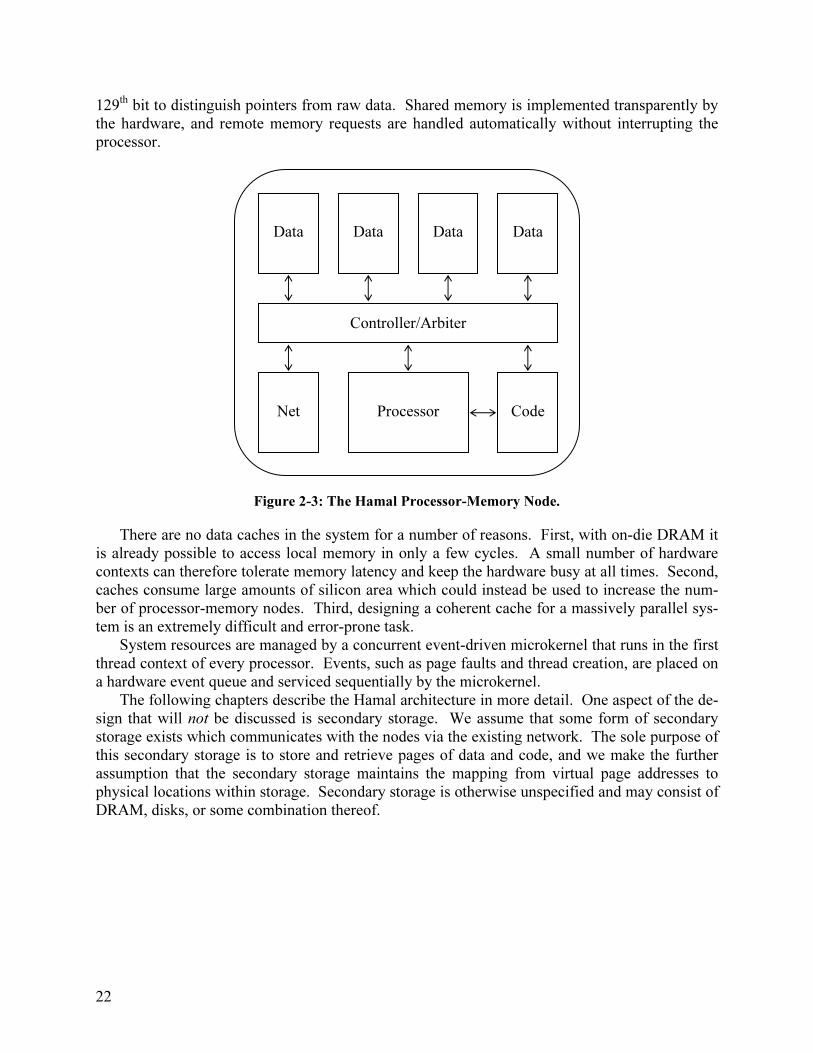
22

129th bit to distinguish pointers from raw data. Shared memory is implemented transparently by the hardware, and remote memory requests are handled automatically without interrupting the processor.

Figure 2-3: The Hamal Processor-Memory Node.

There are no data caches in the system for a number of reasons. First, with on-die DRAM it is already possible to access local memory in only a few cycles. A small number of hardware contexts can therefore tolerate memory latency and keep the hardware busy at all times. Second, caches consume large amounts of silicon area which could instead be used to increase the num-ber of processor-memory nodes. Third, designing a coherent cache for a massively parallel sys-tem is an extremely difficult and error-prone task.

System resources are managed by a concurrent event-driven microkernel that runs in the first thread context of every processor. Events, such as page faults and thread creation, are placed on a hardware event queue and serviced sequentially by the microkernel.

The following chapters describe the Hamal architecture in more detail. One aspect of the de-sign that will not be discussed is secondary storage. We assume that some form of secondary storage exists which communicates with the nodes via the existing network. The sole purpose of this secondary storage is to store and retrieve pages of data and code, and we make the further assumption that the secondary storage maintains the mapping from virtual page addresses to physical locations within storage. Secondary storage is otherwise unspecified and may consist of DRAM, disks, or some combination thereof.

Data

Data

Data

Data

Controller/Arbiter

Code

Net

Processor

23

Chapter 3

The Memory System

The two offices of memory are collection and distribution.

– Samuel Johnson (1709-1784)

In a shared-memory parallel computer, the memory model and its implementation have a direct impact on system performance, programmability and scalability. In this chapter we describe the various aspects of the Hamal memory system, which has been designed to address the specific goals of massive scalability and processor-memory integration.

3.1 Capabilities

If a machine is to support environment-level general purpose computing, one of the first re-quirements of the memory system is that it provide a protection mechanism to prevent applica-tions from reading or writing each other’s data. In a conventional system, this is accomplished by providing each process with a separate virtual address space. While such an approach is func-tional, it has three significant drawbacks. First, a process-dependent address translation mecha-nism dramatically increases the amount of machine state associated with a given process (page tables, TLB entries, etc), which increases system overhead and is an impediment to fine-grained multithreading. Second, data can only be shared between processes at the page granularity, and doing so requires some trickery on the part of the operating system to ensure that the page tables of the various processes sharing the data are kept consistent. Finally, this mechanism does not provide security within a single context; a program is free to create and use invalid pointers.

These problems all stem from the fact that in most architectures there is no distinction at the hardware level between pointers and integers; in particular a user program can create a pointer to an arbitrary location in the virtual address space. An alternate approach which addresses these problems is the use of unforgeable capabilities ([Dennis65], [Fabry74]). Capabilities allow the hardware to guarantee that user programs will make no illegal memory references. It is therefore safe to use a single shared virtual address space which greatly simplifies the memory model.

In the past capability machines have been implemented using some form of capability table ([Houdek81], [Tyner81]) and/or special capability registers ([Abramson86], [Herbert79]), or even in software ([Anderson86], [Chase94]). Such implementations have high overhead and are an obstacle to efficient computing with capabilities. However, in [Carter94] a capability format is proposed in which all relevant address, permission and segment size information is contained in a 64 bit word. This approach obviates the need to perform expensive table lookup operations for every memory reference and every pointer arithmetic operation. Additionally, the elimina-tion of capability tables allows the use of an essentially unbounded number of segments (blocks

24

of allocated memory); in particular object-based protection schemes become practical. The pro-posed format requires all segment sizes to be powers of two and uses six bits to store the base 2 logarithm of the segment size, allowing for segments as small as one byte or as large as the entire address space.

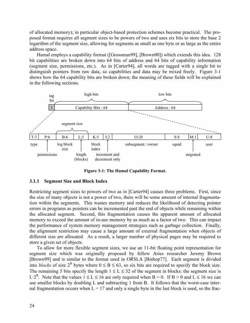
Hamal employs a capability format ([Grossman99], [Brown00]) which extends this idea. 128 bit capabilities are broken down into 64 bits of address and 64 bits of capability information (segment size, permissions, etc.). As in [Carter94], all words are tagged with a single bit to distinguish pointers from raw data, so capabilities and data may be mixed freely. Figure 3-1 shows how the 64 capability bits are broken down; the meaning of these fields will be explained in the following sections.

Figure 3-1: The Hamal Capability Format.

3.1.1 Segment Size and Block Index

Restricting segment sizes to powers of two as in [Carter94] causes three problems. First, since the size of many objects is not a power of two, there will be some amount of internal fragmenta-tion within the segments. This wastes memory and reduces the likelihood of detecting pointer errors in programs as pointers can be incremented past the end of objects while remaining within the allocated segment. Second, this fragmentation causes the apparent amount of allocated memory to exceed the amount of in-use memory by as much as a factor of two. This can impact the performance of system memory management strategies such as garbage collection. Finally, the alignment restriction may cause a large amount of external fragmentation when objects of different size are allocated. As a result, a larger number of physical pages may be required to store a given set of objects.

To allow for more flexible segment sizes, we use an 11-bit floating point representation for segment size which was originally proposed by fellow Aries researcher Jeremy Brown [Brown99] and is similar to the format used in ORSLA [Bishop77]. Each segment is divided

into blocks of size 2B bytes where 0 ≤ B ≤ 63, so six bits are required to specify the block size.

The remaining 5 bits specify the length 1 ≤ L ≤ 32 of the segment in blocks: the segment size is

L·2B. Note that the values 1 ≤ L ≤ 16 are only required when B = 0. If B > 0 and L ≤ 16 we can use smaller blocks by doubling L and subtracting 1 from B. It follows that the worst-case inter-nal fragmentation occurs when L = 17 and only a single byte in the last block is used, so the frac-

T:3 P:6 B:6 L:5 K:5 I:2 O:20 S:8 U:8

permissions

type

length

(blocks)

log block

size

block

index

segment size

increment and

decrement only

subsegment / owner

M:1

squid

migrated

user

1 Capability Bits : 64 Address : 64

high bits low bits tag

bit

25

tion of wasted memory is less than 1/17 < 5.9%. As noted in [Carter94], this is the maximum amount of virtual memory which is wasted; the amount of physical memory wasted will in gen-eral be smaller.

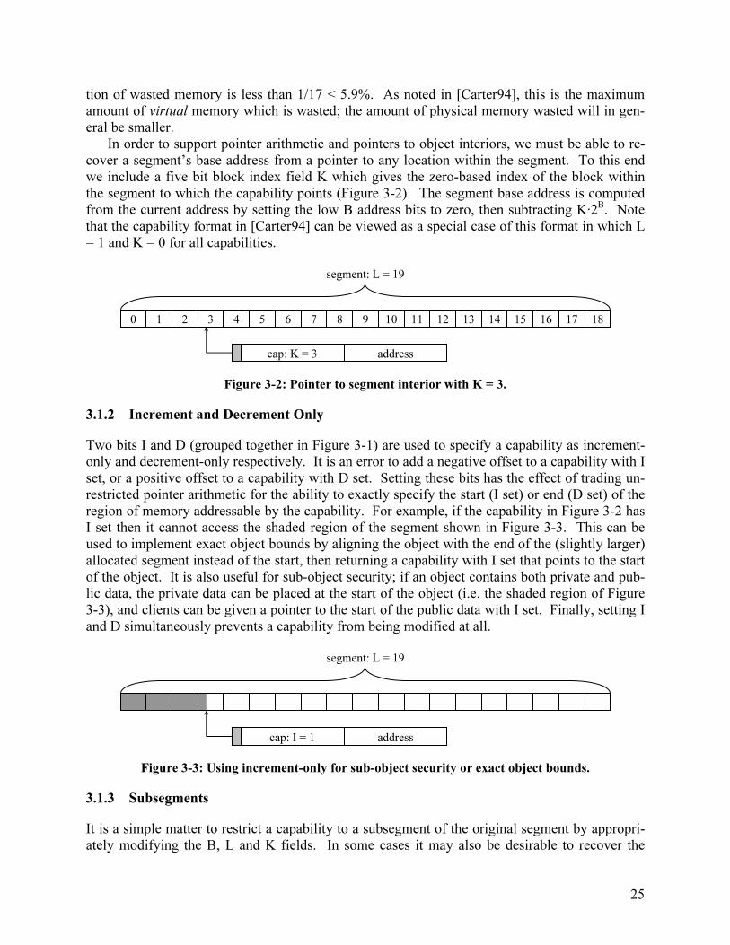
In order to support pointer arithmetic and pointers to object interiors, we must be able to re-cover a segment’s base address from a pointer to any location within the segment. To this end we include a five bit block index field K which gives the zero-based index of the block within the segment to which the capability points (Figure 3-2). The segment base address is computed from the current address by setting the low B address bits to zero, then subtracting K·2B. Note that the capability format in [Carter94] can be viewed as a special case of this format in which L = 1 and K = 0 for all capabilities.

Figure 3-2: Pointer to segment interior with K = 3.

3.1.2 Increment and Decrement Only

Two bits I and D (grouped together in Figure 3-1) are used to specify a capability as increment-only and decrement-only respectively. It is an error to add a negative offset to a capability with I set, or a positive offset to a capability with D set. Setting these bits has the effect of trading un-restricted pointer arithmetic for the ability to exactly specify the start (I set) or end (D set) of the region of memory addressable by the capability. For example, if the capability in Figure 3-2 has I set then it cannot access the shaded region of the segment shown in Figure 3-3. This can be used to implement exact object bounds by aligning the object with the end of the (slightly larger) allocated segment instead of the start, then returning a capability with I set that points to the start of the object. It is also useful for sub-object security; if an object contains both private and pub-lic data, the private data can be placed at the start of the object (i.e. the shaded region of Figure 3-3), and clients can be given a pointer to the start of the public data with I set. Finally, setting I and D simultaneously prevents a capability from being modified at all.

Figure 3-3: Using increment-only for sub-object security or exact object bounds.

3.1.3 Subsegments

It is a simple matter to restrict a capability to a subsegment of the original segment by appropri-ately modifying the B, L and K fields. In some cases it may also be desirable to recover the

segment: L = 19

cap: I = 1 address

0 1 2 3 4 5 6 7 8 9 10 11 12 13 14 15 16 17 18

segment: L = 19

cap: K = 3 address

26

original segment from a restricted capability; a garbage collector, for example, would require this information. We can accomplish this by saving the values of (B, L, K) corresponding to the start of the subsegment within the original segment. Given an arbitrarily restricted capability, the original segment can then be recovered in two steps. First we compute the base address of the sub-segment as described in Section 3.1.1. Then we restore the saved (B, L, K) and again com-pute the base address, this time of the containing segment. Note that we must always store (B, L, K) for the largest containing segment, and if a capability is restricted several times then the in-termediate sub-segments cannot be recovered. This scheme requires 16 bits of storage; these 16 bits are placed in the shared 20-bit subsegment / owner field. The other use for this field will be explained in Section 3.4 when we discuss distributed objects.

3.1.4 Other Capability Fields

The three bit type field (T) is used to specify one of seven hardware-recognized capability types. A data capability is a pointer to data memory. A code capability is used to read or execute code. Two types of sparse capabilities are used for distributed objects and will be described in Section 3.4. A join capability is used to write directly to one or more registers in a thread and will be discussed in Section 4.4. An IO capability is used to communicate with the external host. Fi-nally, a user capability has a software-specified meaning, and can be used to implement unforge-able certificates.

The permissions field (P) contains the following permission bits:

Bit Permission

R read

W write

T take

G grant

DT diminished take

DG diminished grant

X execute

P execute privileged

Table 3-1: Capability permission bits

The read and write bits allow the capability to be used for reading/writing non-pointer data; take and grant are the corresponding permission bits for reading/writing pointers. The dimin-ished take and diminished grant bits also allow capabilities to be read/written, however they are “diminished” by clearing all permission bits except for R and DT. These permission bits are based on those presented in [Karger88]. The X and P bits are exclusively for code capabilities which do not use the W, T, G, DT or DG bits (in particular, Hamal specifies that code is read-only). Hence, only 6 bits are required to encode the above permissions.

The eight bit user field (U) is ignored by the hardware and is available to the operating sys-tem for use. Finally, the eight bit squid field (S) and the migrated bit (M) are used to provide support for forwarding pointers as described in the next section.

27

3.2 Forwarding Pointer Support

Forwarding pointers are a conceptually simple mechanism that allow references to one memory

location to be transparently forwarded to another. Known variously as “invisible pointers”

[Greenblatt74], “forwarding addresses” [Baker78] and “memory forwarding” [Luk99], they are

relatively easy to implement in hardware, and are a valuable tool for safe data compaction

([Moon84], [Luk99]) and object migration [Jul88]. Despite these advantages, however, forward-

ing pointers have to date been incorporated into few architectures.

One reason for this is that forwarding pointers have traditionally been perceived as having

limited utility. Their original intent was fairly specific to LISP garbage collection, but many

methods of garbage collection exist which do not make use of or benefit from forwarding point-

ers [Plainfossé95], and consequently even some LISP-specific architectures do not implement

forwarding pointers (such as SPUR [Taylor86]). Furthermore, the vast majority of processors

developed in the past decade have been designed with C code in mind, so there has been little

reason to support forwarding pointers.

More recently, the increasing prevalence of the Java programming language has prompted in-

terest in mechanisms for accelerating the Java virtual machine, including direct silicon imple-

mentation [Tremblay99]. Since the Java specification includes a garbage collected memory

model [Gosling96], architectures designed for Java can benefit from forwarding pointers which

allow efficient incremental garbage collection ([Baker78], [Moon84]). Additionally, in [Luk99]

it is shown that using forwarding pointers to perform safe data relocation can result in significant

performance gains on arbitrary programs written in C, speeding up some applications by more

than a factor of two. Finally, in a distributed shared memory machine, data migration can im-

prove performance by collocating data with the threads that require it. Forwarding pointers pro-

vide a safe and efficient mechanism for object migration [Jul88]. Thus, there is growing motiva-

tion to include hardware support for forwarding pointers in novel architectures.

A second and perhaps more significant reason that forwarding pointers have received little

attention from hardware designers is that they create a new set of aliasing problems. In an archi-

tecture that supports forwarding pointers, no longer can the hardware and programmer assume

that different pointers point to different words in memory (Figure 3-4). In [Luk99] two specific

problems are identified. First, direct pointer comparisons are not a safe operation; some mecha-

nism must be provided for determining the final addresses of the pointers. Second, seemingly

independent memory operations may no longer be reordered in out-of-order machines.

Figure 3-4: Aliasing resulting from forwarding pointer indirection.

data (D)

forwarding pointer to D

P2: direct pointer to D

P1: indirect pointer to D

28

3.2.1 Object Identification and Squids

Forwarding pointer aliasing is an instance of the more general challenge of determining object identity in the presence of multiple and/or changing names. This problem has been studied ex-plicitly [Setrag86]. A natural solution which has appeared time and again is the use of system-wide unique object ID’s (e.g. [Dally85], [Setrag86], [Moss90], [Day93], [Plainfossé95]). UID’s completely solve the aliasing problem, but have two disadvantages:

i. The use of ID’s to reference objects requires an expensive translation each time an object is referenced to obtain its virtual address.

ii. Quite a few bits are required to ensure that there are enough ID’s for all objects and that

globally unique ID’s can be easily generated in a distributed computing environment. In a large system, at least sixty-four bits would likely be required in order to avoid any ex-pensive garbage collection of ID’s and to allow each processor to allocate ID’s independ-ently.

Despite these disadvantages, the use of ID’s remains appealing as a way of solving the alias-

ing problem, and it is tempting to try to find a practical and efficient mechanism based on ID’s. We begin by noting that the expensive translations (i) are unnecessary if object ID’s are included as part of the capability format. In this case we have the best of both worlds: object references make use of the address so that no translation is required, and pointer comparisons and memory operation reordering are based on ID’s, eliminating aliasing problems. However, this still leaves us with disadvantage (ii), which implies that the pointer format must be quite large.

We can solve this problem by dropping the restriction that the ID’s be unique. Instead of long unique ID’s, we use short quasi-unique ID’s (squids) [Grossman02]. At first this seems to defeat the purpose of having ID’s, but we make the following observation: while squids cannot be used to determine that two pointers reference the same object, they can in most cases be used to determine that two pointers reference different objects. If we randomly generate an n bit squid every time an object is allocated, then the probability that pointers to distinct objects cannot be distinguished by their squids is 2-n.

3.2.2 Pointer Comparisons and Memory Operation Reordering

We can efficiently compare two pointers by comparing their base addresses, their segment off-sets and their squids. If the base addresses are the same then the pointers point to the same ob-ject, and can be compared using their offsets. If the squids are different then they point to differ-ent objects. If the offsets are different then they either point to different objects or to different words of the same object. In the case that the base addresses are different but the squids and off-sets are the same, we trap to a software routine which performs the expensive dereferences nec-essary to determine whether or not the final addresses are equal.

We can argue that this last case is rare by observing that it occurs in two circumstances: ei-ther the pointers reference different objects which have the same squid, or the pointers reference the same object through different levels of indirection. The former occurs with probability 2-n. The latter is application dependent, but we note that (1) applications tend to compare pointers to different objects more frequently then they compare pointers to the same object, and (2) the re-sults of the simulations in [Luk99] indicate that it may be reasonable to expect the majority of

29

pointers to migrated data to be updated, so that two pointers to the same object will usually have the same level of indirection.

In a similar manner, the hardware can use squids to decide whether or not it is possible to re-order memory operations. If the squids are different, it is safe to reorder. If the squids are the same but the offsets are different, it is again safe to reorder. If the squids and offsets are the same but the addresses are different, the hardware assumes that the operations cannot be reor-dered. It is not necessary to explicitly check for aliasing since preserving order guarantees con-servative but correct execution. Only simple comparisons are required, and the probability of failing to reorder references to different objects is 2-n.

3.2.3 Implementation

The Hamal capability contains an eight bit squid field (S) which is randomly generated every time memory is allocated. The probability that two objects cannot be distinguished by their squids is thus 2-8 < 0.4%. This reduces the overhead due to aliasing to a small but still non-zero amount. In order to eliminate overhead completely for applications that do not make use of for-warding pointers, we add a migrated bit (M) which indicates whether or not the capability points to the original segment of memory in which the object was allocated. When a new object is cre-ated, pointers to that object have M = 0. When the object is migrated, pointers to the new loca-tion (and all subsequent locations) have M = 1. If the hardware is comparing two pointers with M = 0 (either as the result of a comparison instruction, or to check for a dependence between memory operations), it can ignore the squids and perform the comparison based on addresses alone. Hence, there is no runtime cost associated with support for forwarding pointers if an ap-plication does not use them.

3.3 Augmented Memory

One of the goals of this thesis is to explore ways in which embedded DRAM technology can be leveraged to migrate various features and computational tasks into memory. The following sec-tions describe a number of augmentations to memory in the Hamal architecture.

3.3.1 Virtual Memory

The memory model of early computers was simple: memory was external storage for data; data could be modified or retrieved by supplying the memory with an appropriate physical address. This model was directly implemented in hardware by discrete memory components. Such a sim-plified view of memory has long since been replaced by the abstraction of virtual memory, yet the underlying memory components have not changed. Instead, complexity has been added to processors in the form of logic which performs translations from sophisticated memory models to simple physical addresses.

There are a number of drawbacks to this approach. The overhead associated with each mem-ory reference is large due to the need to look up page table entries. All modern processors make use of translation lookaside buffers (TLB’s) to try to avoid the performance penalties associated with these lookups. A TLB is essentially a cache, and as such provides excellent performance for programs that use sufficiently few pages, but is of little use to programs whose working set of pages is large. Another problem common to any form of caching is the “pollution” that occurs in a multi-threaded environment: a single TLB must be shared by all threads which reduces its ef-

30

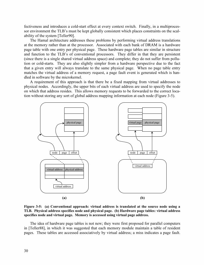
fectiveness and introduces a cold-start effect at every context switch. Finally, in a multiproces-sor environment the TLB’s must be kept globally consistent which places constraints on the scal-ability of the system [Teller90].

The Hamal architecture addresses these problems by performing virtual address translations at the memory rather than at the processor. Associated with each bank of DRAM is a hardware page table with one entry per physical page. These hardware page tables are similar in structure and function to the TLB’s of conventional processors. They differ in that they are persistent (since there is a single shared virtual address space) and complete; they do not suffer from pollu-tion or cold-starts. They are also slightly simpler from a hardware perspective due to the fact that a given entry will always translate to the same physical page. When no page table entry matches the virtual address of a memory request, a page fault event is generated which is han-dled in software by the microkernel.

A requirement of this approach is that there be a fixed mapping from virtual addresses to physical nodes. Accordingly, the upper bits of each virtual address are used to specify the node on which that address resides. This allows memory requests to be forwarded to the correct loca-tion without storing any sort of global address mapping information at each node (Figure 3-5).

Figure 3-5: (a) Conventional approach: virtual address is translated at the source node using a

TLB. Physical address specifies node and physical page. (b) Hardware page tables: virtual address

specifies node and virtual page. Memory is accessed using virtual page address.

The idea of hardware page tables is not new; they were first proposed for parallel computers in [Teller88], in which it was suggested that each memory module maintain a table of resident pages. These tables are accessed associatively by virtual address; a miss indicates a page fault.

virtual address physical address

node page offset

virtual address

physical page virtual page physical page

node page offset

virtual address

(a) (b)

31

Subsequent work has verified the performance advantages of translating virtual addresses to

physical addresses at the memory rather than at the processor ([Teller94], [Qui98], [Qui01]).

A related idea is inverted page tables ([Houdek81], [Chang88], [Lee89]) which also feature a

one to one correspondence between page table entries and physical pages. However, the inten-

tion of inverted page tables is simply to support large address spaces without devoting massive

amounts of memory to traditional forward-mapped page tables. The page tables still reside in

memory, and translation is still performed at the processor. A hash table is used to locate page

table entries from virtual addresses. In [Huck93], this hash table is combined with the inverted

page table to form a hashed page table.

3.3.2 Automatic Page Allocation

Hardware page tables allow the memory banks to detect which physical pages are in use at any

given time. A small amount of additional logic makes it possible for them to select an unused

page when one is required. In the Hamal architecture, when a virtual page is created or paged in,

the targeted memory bank automatically selects a free physical page and creates the page table

entry. Additionally, pages that are created are initialized with zeros. The combination of hard-

ware page tables and automatic page allocation obviates the need for the kernel to ever deal with

physical page numbers, and there are no instructions that allow it to do so.

3.3.3 Hardware LRU

Most operating systems employ a Least Recently Used (LRU) page replacement policy. Typi-

cally the implementation is approximate LRU rather than exact LRU, and some amount of work

is required by the operating system to keep track of LRU information and determine the LRU

page. In the Hamal architecture, each DRAM bank automatically maintains exact LRU informa-

tion. This simplifies the operating system and improves performance; a lengthy sequence of

status bit polling to determine LRU information is replaced by a single query which immediately

returns an exact result. To provide some additional flexibility, each page may be assigned a

weight in the range 0-127; an LRU query returns the LRU page of least weight.

3.3.4 Atomic Memory Operations

The ability to place logic and memory on the same die produces a strong temptation to engineer

“intelligent” memory by adding some amount of processing power. However, in systems with

tight processor/memory integration there is already a reasonably powerful processor next to the

memory; adding an additional processor would do little more than waste silicon and confuse the

compiler. The processing performed by the memory in the Hamal architecture is therefore lim-

ited to simple single-cycle atomic memory operations such as addition, maximum and boolean

logic. These operations are useful for efficient synchronization and are similar to those of the

Tera [Alverson90] and CrayT3E [Scott96] memory systems.

3.3.5 Memory Traps and Forwarding Pointers

Three trap bits (T, U, V) are associated with every 128 bit data memory word. The meaning of

the T bit depends on the contents of the memory word. If the word contains a valid data pointer,

the pointer is interpreted as a forwarding pointer and the memory request is automatically for-

warded. Otherwise, references to the memory location will cause a trap. This can be used by the

32

operating system to implement mechanisms such as data breakpoints. The U and V bits are

available to user programs to enrich the semantics of memory accesses via customized trapping

behaviour. Each instruction that accesses memory specifies how U and V are interpreted and/or

modified. For each of U and V, the possible behaviours are to ignore the trap bit, trap on set, and

trap on clear. Each trap bit may be left unchanged, set, or cleared, and the U bit may also be

toggled. When a memory request causes a trap the contents of the memory word and its trap bits

are left unchanged and an event is generated which is handled by the microkernel. The T trap bit

is also associated with the words of code memory (each 128 bit code memory word contains one

VLIW instruction) and can be used in this context to implement breakpoints.

The U and V bits are a generalization of the trapping mechanisms implemented in HEP

[Smith81], Tera [Alverson90], and Alewife [Kranz92]. They are also similar to the pre- and

post-condition mechanism of the M-Machine [Keckler98], which differs from the others in that

instead of causing a trap, a failure sets a predicate register which must be explicitly tested by the

user program.

Handling traps on the node containing the memory location rather than on the node contain-

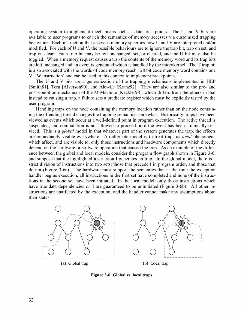
ing the offending thread changes the trapping semantics somewhat. Historically, traps have been

viewed as events which occur at a well-defined point in program execution. The active thread is

suspended, and computation is not allowed to proceed until the event has been atomically ser-

viced. This is a global model in that whatever part of the system generates the trap, the effects

are immediately visible everywhere. An alternate model is to treat traps as local phenomena

which affect, and are visible to, only those instructions and hardware components which directly

depend on the hardware or software operation that caused the trap. As an example of the differ-

ence between the global and local models, consider the program flow graph shown in Figure 3-6,

and suppose that the highlighted instruction I generates an trap. In the global model, there is a

strict division of instructions into two sets: those that precede I in program order, and those that

do not (Figure 3-6a). The hardware must support the semantics that at the time the exception

handler begins execution, all instructions in the first set have completed and none of the instruc-

tions in the second set have been initiated. In the local model, only those instructions which

have true data dependencies on I are guaranteed to be uninitiated (Figure 3-6b). All other in-

structions are unaffected by the exception, and the handler cannot make any assumptions about

their states.

Figure 3-6: Global vs. local traps.

I I

(a) Global trap (b) Local trap

33

The local model is better suited to parallel and distributed computing, in which the execution

of a single thread may be physically distributed across the machine; it is the model used in the

Hamal architecture. With a global trapping model, a thread would have to stall on every remote

memory reference. Memory references causing a trap would be returned to the processor where

the thread would be preempted by a trap handler. With a local exception model, a thread may

continue processing while waiting for a remote memory reference to complete. If the reference

causes a trap, the trap is serviced on the remote node, independent of the thread that caused it,

and the trap handler completes the memory request manually. This is transparent to the thread;

the entire sequence is indistinguishable from an unusually long-latency memory operation.

To allow for application-dependent trapping behaviour, each memory request which can po-

tentially trap on the U and V bits is accompanied by the requesting thread’s trap vector, a code

capability giving the entry point to a trap handler. The microkernel responds to U and V trap

events by creating a new thread to run the trap handler.

3.4 Distributed Objects

In large-scale shared-memory systems, the layout of data in physical memory is crucial to

achieving the best possible performance. In particular, for many algorithms it is important to be

able to allocate single objects in memory which are distributed across multiple nodes in the sys-

tem. The challenge is to allow arbitrary single nodes to perform such allocations without any

global communication or synchronization. A straightforward approach is to give each node own-

ership of parts of the virtual address space that exist on all other nodes, but this makes poor use

of the virtual address bits: an N node system would require 2logN bits of virtual address to

specify both location and ownership.

In this section we describe two different approaches to distributed object allocation: Extended

Address Partitioning and Sparsely Faceted Arrays [Brown02a]. These techniques share the

characteristic that a node atomically and without communication allocates a portion of the virtual

address space - a facet - on each node in the system, but actual physical memory is lazily allo-

cated only on those nodes which make use of the object. Both of these mechanisms have been

incorporated into the Hamal architecture.

3.4.1 Extended Address Partitioning

Consider a simple system which gives each node ownership of a portion of the virtual address

space on all other nodes, using logN virtual address bits to specify ownership (Figure 3-7a).

When a distributed object is allocated, these logN bits are set to the ID of the node on which the

allocation was performed. Thereafter, the owner bits are immutable. Pointer arithmetic on ca-

pabilities for the object may alter the node and address fields, but not the owner field. We can

therefore move the owner field from the address bits to the capability bits (Figure 3-7b). This

has the effect of extending the virtual address space by logN bits, then partitioning it so that each

node has ownership of, and may allocate segments within, an equal portion of the address space.

34

Figure 3-7: (a) Simple address partitioning. (b) Extended address partitioning.

Distributed objects are allocated using extended address partitioning by reserving the same

address range on all nodes. Capabilities for these objects are of type sparse; the term “sparse”

reflects the fact that while an object is conceptually allocated on all nodes, its facets may physi-

cally exist only on a small subset of nodes. There are two differences between sparse capabili-

ties and data capabilities. First, when a sparse capability is created the owner field is automati-

cally set (recall that the owner field is used for subsegments in data capabilities; subsegmenting

of a sparse capability is not allowed). Second, the node field of the address may be altered freely

using pointer arithmetic or indexing. The remaining capability fields have the same meaning in

both capability types. In particular B, L and K have the same values that they would if the speci-

fied address range had been allocated on a single node only.

In a capability architecture such as Hamal, no special hardware mechanism is required to im-

plement lazy allocation of physical memory; it suffices to make use of page faults. This is be-

cause capabilities guarantee that all pointers are valid, so a page fault on a non-existent page al-

ways represents a page that needs to be created and initialized, and never represents an applica-

tion error. As a result, no communication needs to take place between the allocating node and

the nodes on which the object is stored other than the capability itself, which is included in

memory requests involving the object.

3.4.2 Sparsely Faceted Arrays

A problem with extended address partitioning is that the facets of distributed objects allocated by

different nodes must reside in different physical pages, which can result in significant fragmenta-

tion and wasted physical memory. This is illustrated by Figure 3-8a, which shows how the facets

of four distributed objects allocated by four different nodes are stored in memory on a fifth node.

Four pages are required to store the facets, and most of the space in these pages is unused.

Figure 3-8: (a) Extended address partitioning results in fragmentation. (b) Address translation

allows facets to be allocated contiguously.

1:0x10000

3:0x10000

4:0x10000

6:0x10000

48

16

96

64

base

owner:address

size

(bytes)

1:0x10000

3:0x10000

4:0x10000

6:0x10000

48

16

96

64

global base

owner:address

size

(bytes)

0x20000

local

address

0x20040

0x20050

0x200b0

1:0x10000

3:0x10000

4:0x10000

6:0x10000

0x20000

Distributed Objects Global → Local TranslationsNode 7 pages Node 7 pages

(a) (b)

node owner address node owner address

capability bits address bits capability bits address bits

(a) (b)

35

Sparsely faceted arrays (SFAs) are a solution to this problem described in [Brown02a]. The

central idea is to perform a translation from global array names (which consist of the owner node

and the base address on that node) to local addresses. This extra layer of translation allows fac-

ets to be allocated contiguously, even intermingled with local data, regardless of the nodes on

which the SFAs were allocated (Figure 3-8b).

SFAs require a translation table to exist at the boundary of each processing node in order to

translate local addresses to/from global array names. When a SFA pointer moves from a node to

the network, it is first decomposed into a base address and an offset. The base address is used to

look up the array’s global name in the translation table. Similarly, when a SFA pointer arrives at

a node, the owner and base address are used to look up the local facet base address in the transla-

tion table. If no entry exists in the table, which occurs the first time a node sees a pointer to a

given SFA, then a local facet is allocated and the base address is entered into the table. Note that

no translation is required at the boundary of the owner node.

SFA capabilities in the Hamal architecture have type translated sparse, or xsparse. They are

exactly the same as sparse capabilities, and are only treated differently by the network interface

which recognizes them and automatically performs translations. In particular, the owner field is

still set automatically when an xsparse capability is created. While this is not strictly necessary

for a SFA implementation, it has two advantages. First, it allows the network interface to detect

xsparse capabilities that are locally owned, so the null local ↔ global translation for this case

can be omitted from the translation table. Second, it avoids the need to expand xsparse capabili-

ties from 128 to 128 + logN bits to include the owner node when they are transmitted across the

network. Each network interface has a 256-entry translation cache and can perform a single

translation on each cycle. In the case of a cache miss, an event is generated which must be han-

dled by the microkernel.

3.4.3 Comparison of the Two Approaches

Each of these approaches has benefits and disadvantages. Extended address partitioning has very

low overhead and is inherently scalable. It has the additional advantage of enlarging the virtual

address space. However, it can suffer from significant fragmentation problems. Sparsely faceted

arrays eliminate fragmentation, but require translation tables to be stored at individual nodes

which can potentially affect the scalability of the system. These tables do not store global infor-

mation as translations are locally generated and managed, but it is not clear how quickly they

will grow over time or with machine size, and some sort of translation garbage collection would

be required to prevent the tables from becoming arbitrarily large. Another issue is the perform-

ance degradation which occurs if the working set of SFAs on some node exceeds the size of the

hardware translation table. It is impossible to determine a priori which approach is to be pre-

ferred; most likely this is application-dependent. We have therefore chosen to implement both

mechanisms in the Hamal architecture.

3.4.4 Data Placement

If an application programmer has specific knowledge concerning the physical layout of the proc-

essor nodes and the topology of the network that connects them, it may be desirable to specify

not only that an object is to be distributed, but also the exact mapping of facets to physical nodes.

The ability to do so has been integrated into the High Performance Fortran language [Koel-

bel94], and some parallel architectures provide direct hardware support. The M-Machine has a

36

global translation mechanism which allows large portions of the virtual address space to be

mapped over rectilinear subsets of the system’s three dimensional array of nodes [Dally94b]. In

the Tera Computer System, consecutive virtual addresses in a segment may be distributed among

any power of two number of memory units [Alverson90]. The Cray T3E features an address

centrifuge which can extract user-specified bits from a virtual address and use them to form the

ID for the node on which the data resides [Scott96].

The Hamal processor contains no global segment or translation tables; virtual addresses are

routed to physical nodes based exclusively on the upper address bits. To compensate for this

somewhat rigid mapping and to allow applications to lay out an object in a flexible manner with-

out performing excessive computation on indices, a hardware swizzle instruction is provided.

This instruction combines a 64 bit operand with a 64 bit mask to produce a 64 bit result by right-

compacting the operand bits corresponding to 1’s in the mask, and left-compacting the operand

bits corresponding to 0’s in the mask. swizzle is a powerful bit-manipulation primitive with a

number of potential uses. In particular, it allows an address centrifuge to be implemented in

software using a single instruction.

3.5 Memory Semantics

Sequential consistency presents a natural and intuitive shared memory model to the programmer.

Unfortunately, it also severely restricts the performance of many parallel applications

([Gharach91], [Zucker92], [Chong95]). This is due to the fact that no memory operation from a

given thread may proceed until the effect of every previous memory operation from that thread is

globally visible in the machine. This problem becomes worse as machine size scales up and the

average round trip time for a remote memory reference increases.

In order to maximize program efficiency, Hamal makes no guarantees concerning the order

in which references to different memory locations complete. Memory operations are explicitly

split-phase; a thread continues to execute after a request is injected into the system, and at some

unknown time in the future a reply will be received. The hardware will only force a thread to

stall in three circumstances:

1. The result of a read is needed before a reply containing the value is received

2. There is a RAW, WAR or WAW hazard with a previous memory operation

3. The hardware table used to keep track of incomplete memory operations is full

A wait instruction is provided to force a thread to stall until all outstanding memory opera-

tions have completed. This allows release consistency [Gharach90] to be efficiently imple-

mented in software.

37

Chapter 4

Processor Design

Everything should be made as simple as possible, but not simpler.

– Albert Einstein (1879-1955)

The Hamal architecture features 128 bit multithreaded Very Long Instruction Word (VLIW)

processors. There are eight hardware contexts; of these, context 0 is reserved for the event-

driven microkernel, and contexts 1-7 are available for running user programs. Instructions may

be issued from a different context on each cycle, and instructions from multiple contexts may

complete in a given cycle. Each context consists of an instruction cache, a trace controller

(which fetches instructions from the instruction cache and executes control flow instructions),

issue logic, 32 128-bit tagged general purpose registers, 15 single-bit predicate registers, and a

small number of special-purpose registers.

Each VLIW instruction group consists of three instructions and an immediate. One instruc-

tion is an arithmetic instruction which specifies up to two source operands and a destination reg-

ister. One instruction is a memory instruction which specifies up to three source operands (ad-

dress, index, data) and a destination register; this can also be a second arithmetic instruction for

certain simple single-cycle operations. The last instruction is a control flow instruction which

specifies zero or one operands. Predicated execution is supported; each instruction within an in-

struction group can be independently predicated on the value (true or false) of any one the 15

predicates.

This chapter gives an overview of, and provides motivation for, the key features of the

Hamal processor. These features represent various tradeoffs involving the five design principles

outlined in Section 2.1: scalability, silicon efficiency, simplicity, programmability, and perform-

ance. A more detailed description of the processor can be found in [Grossman01a] and

[Grossman01b].

4.1 Datapath Width and Multigranular Registers

The choice of 128 bits as the basic datapath and register width was motivated by two factors:

1. Capabilities are 128 bits, so at least some datapaths must be this wide

2. Wide datapaths make effective use of the available embedded DRAM bandwidth

A criticism of wide datapaths is that large portions of the register file and/or functional units

will be unused for applications which deal primarily with 32 or 64 bit data, significantly reducing

the area efficiency of the processor. This issue is addressed in two ways. First, each register is

38

addressable as a single 128 bit register, two 64 bit registers, or four 32 bit registers (Figure 4-1).

This requires a small amount of shifting logic to implement in hardware, and increases both the

register file utilization and the number of registers available to user programs. Second, many of

the instructions can operate in parallel on two sets of 64 bit inputs or four sets of 32 bit inputs

packed into 128 bits. This provides the opportunity to increase both performance and functional

unit usage via fine-grained SIMD parallelism. Note that, for the purpose of scoreboarding, busy

bits must be maintained for the finest register granularity; a register is marked as busy by setting

the busy bits of all of its sub-registers.

r3 r2y r2x r1y r1b r1a r0d r0c r0b r0a

r7 r6 r5 r4

r11 r10 r9 r8

r15 r14 r13 r12

o

Figure 4-1: Multigranular general purpose registers.

4.2 Multithreading and Event Handling

Multithreading is a very well known technique. In [Agarwal92] and [Thekkath94] it is shown

that hardware multithreading can significantly improve processor utilization. A large number of

designs have been proposed and/or implemented which incorporate hardware multithreading;

examples include HEP [Smith81], Horizon [Thistle88], MASA [Halstead88], Tera [Alverson90],

April [Agarwal95], and the M-Machine [Dally94b]. Most of these designs are capable of execut-

ing instructions from a different thread on every cycle, allowing even single-cycle pipeline bub-

bles in one thread to be filled by instructions from another. An extreme model of multithreading,

variously proposed as processor coupling [Keckler92], parallel multithreading [Hirata92] and

simultaneous multithreading [Tullsen95], allows multiple threads to issue instructions during the

same cycle in a superscalar architecture. This has been implemented in the Intel Pentium 4 Xeon

architecture [Marr02].

The idea of using multithreading to handle events is also not new. It is described in both

[Keckler99] and [Zilles99], and has been implemented in the M-Machine [Dally94b]. Using a

separate thread to handle events has been found to provide significant speedups. In [Keckler99]

these speedups are attributed to three primary factors:

1. No instructions need to be squashed

2. No contexts need to be saved and subsequently restored

3. Threads may continue to execute concurrently with the event handler

In the Hamal architecture, events are placed in a hardware event queue. Events may be gen-

erated by memory (e.g. page faults), the network interface (e.g. xsparse translation cache misses)

or by the processor itself (e.g. thread termination). The size of the event queue is monitored in

hardware; if it grows beyond a high-water mark, certain processor activities are throttled to pre-

vent new events from being generated, thus avoiding event queue overflow and/or deadlock. A

special poll instruction allows context 0 to remove an event from the queue; information con-

cerning the event is placed in read-only event registers. The Hamal event-handling model is il-

lustrated in Figure 4-2.

39

Figure 4-2: Event queue and event handler context.

4.3 Thread Management

One of the requirements for efficient fine-grained parallelism is a set of lightweight mechanisms

for thread management. This is made possible in the Hamal architecture via hardware support

for thread swap pages. Each thread is explicitly assigned to a page in memory; the virtual ad-

dress of this page is used to identify the thread. All major thread management operations are

performed by single instructions, issued from context 0, which specify a thread swap address as

their argument. Context loading and unloading is performed in the background while the

processor continues to execute instructions, as described in [Soundarar92].

4.3.1 Thread Creation

Threads are created in the Hamal architecture using a fork instruction which specifies a code

starting address for the new thread and a subset of the 32 general purpose registers to copy into

the thread. The upper bits of the starting address indicate the node on which the new thread

should be created (code capabilities, like sparse capabilities, allow the node field of the address

to be changed via pointer arithmetic and indexing). When a fork request has arrived at the desti-

nation node (which may be the same node that issued the fork instruction), it is placed in a hard-

ware fork queue. Each node has an eight-entry FIFO queue for storing fork requests; when the

queue fills fork instructions on that node are not allowed to issue, and fork packets received from

the network cannot be processed. Each time a fork is placed in the queue a fork event is gener-

ated. The microkernel can handle this event in one of two ways: it can issue an fload instruction

to immediately load the new thread into a free context and activate it, or it can issue an fstore in-

struction to write the new thread to memory. Both of these instructions specify as their single

operand a swap address for the new thread.

4.3.2 Register Dribbling and Thread Suspension

One of the challenges of fine-grained parallelism is deciding when a thread should be suspended;

it is not even clear whether this decision should be made by hardware or software. The problem

is that it is difficult or impossible to predict how long a blocked thread will remain inactive, par-

ticularly in a shared-memory system with no bounds on the amount of time required for a remote

access to complete. In order to minimize the likelihood of suspending a thread that would have

become unblocked a short time in the future while at the same time attempting to keep the proc-

Handle

event

Poll

queue

Event Queue

Memory Events

Processor Events

Network Events

Context 0

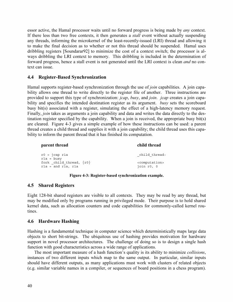
40

essor active, the Hamal processor waits until no forward progress is being made by any context.

If there less than two free contexts, it then generates a stall event without actually suspending

any threads, informing the microkernel of the least-recently-issued (LRI) thread and allowing it

to make the final decision as to whether or not this thread should be suspended. Hamal uses

dribbling registers [Soundarar92] to minimize the cost of a context switch; the processor is al-

ways dribbling the LRI context to memory. This dribbling is included in the determination of

forward progress, hence a stall event is not generated until the LRI context is clean and no con-

text can issue.

4.4 Register-Based Synchronization

Hamal supports register-based synchronization through the use of join capabilities. A join capa-

bility allows one thread to write directly to the register file of another. Three instructions are

provided to support this type of synchronization: jcap, busy, and join. jcap creates a join capa-

bility and specifies the intended destination register as its argument. busy sets the scoreboard

busy bit(s) associated with a register, simulating the effect of a high-latency memory request.

Finally, join takes as arguments a join capability and data and writes the data directly to the des-

tination register specified by the capability. When a join is received, the appropriate busy bit(s)

are cleared. Figure 4-3 gives a simple example of how these instructions can be used: a parent

thread creates a child thread and supplies it with a join capability; the child thread uses this capa-

bility to inform the parent thread that it has finished its computation.

parent thread

r0 = jcap r1ar1a = busyfork _child_thread, {r0}r1a = and r1a, r1a

child thread

_child_thread:

<computation>join r0, 0

Figure 4-3: Register-based synchronization example.

4.5 Shared Registers

Eight 128-bit shared registers are visible to all contexts. They may be read by any thread, but

may be modified only by programs running in privileged mode. Their purpose is to hold shared

kernel data, such as allocation counters and code capabilities for commonly-called kernel rou-

tines.

4.6 Hardware Hashing

Hashing is a fundamental technique in computer science which deterministically maps large data

objects to short bit-strings. The ubiquitous use of hashing provides motivation for hardware

support in novel processor architectures. The challenge of doing so is to design a single hash

function with good characteristics across a wide range of applications.

The most important measure of a hash function’s quality is its ability to minimize collisions,

instances of two different inputs which map to the same output. In particular, similar inputs

should have different outputs, as many applications must work with clusters of related objects

(e.g. similar variable names in a compiler, or sequences of board positions in a chess program).

41

While the meaning of “similar inputs” is application-dependent, one simple metric that can be

applied in any circumstance is hamming distance; the number of bits in which two inputs differ.

We define the minimum collision distance of a hash function to be the smallest positive integer d

such that there exist two inputs separated by hamming distance d that map to the same output.

For an n bit input, m bit output hash function, the goal is to maximize the minimum collision

distance. The problem is that the number of required input and output bits varies greatly from

application to application. A hardware hash function must therefore choose n and m large

enough so that applications can simply use as many of the least significant input and output bits

as they need. It is therefore not enough to ensure that this n → m hash function has a good mini-

mum collision distance, for if the outputs of two similar inputs differ only in their upper bits,

then these two inputs will collide in applications that discard the upper output bits.

In this section we will show how to construct a single n → m hash function which is easy to

implement in hardware and has the property that the n → m’ subhashes obtained by discarding

the upper m – m’ output bits all have good minimum collision distances. Our approach is to con-

struct a nested sequence of linear codes; we will begin with a brief review of these codes and

their properties. Note that it suffices to consider the size of the outputs, as any n’ → m subhash

obtained by forcing a set of n – n’ input bits to zero will have a minimum collision distance at

least as large as that of the original n → m hash.

4.6.1 A Review of Linear Codes

An (n, k) binary linear code C is a k-dimensional subspace of GF(2)n. A generator matrix is any

kxn matrix whose rows form a basis of C. A generator matrix G defines a mapping from k-

dimensional input vectors to code words; given a k-dimensional row vector v, the corresponding

code word is vG. A parity check matrix is any (n − k)xn matrix whose rows form a basis of C⊥,

the subspace of GF(2)n orthogonal to C. A parity check matrix H has the property that an n-

dimensional vector w is a code word if and only if wHT = 0.

The minimum distance of a code is the smallest hamming distance d between two different

code words. For a binary linear code, this is also equal to the smallest weight (number of 1’s) of

any non-zero code word. The quality of a code is determined by its minimum distance, as this

dictates the number of single-bit errors that can be tolerated when code words are communicated

over a noisy channel. Maximizing d for a particular n and k is an open problem, with upper lim-

its given by the non-constructive Johnson bound [Johnson62]. The best known codes tend to

come from the Bose-Chaudhury-Hocquenghem (BCH) [Kasami69] or Extended BCH [Edel97]

constructions.

A BCH code with minimum distance d is constructed as follows. Choose n odd, and choose

q such that n divides 2q – 1. Let β be an order n element of GF(2

q), and let j be an integer rela-

tively prime to n. Finally, let g be the least common multiple of the minimal polynomials of β j,

β j + 1, β j + 2

, …, β j + d – 2 over GF(2). The code words are then the coefficients of the polynomi-

als over GF(2) with degree < n which are divisible by g. If g has degree m, this defines an

(n, n − m) linear code with minimum distance ≥ d.

4.6.2 Constructing Hash Functions from Linear Codes

Let H be a parity check matrix for an (n, k, d) linear code (the third parameter in this notation is

the minimum distance). Let H() be the linear n → k hash function defined by H(v) = vHT. For

42

any two input vectors x and y, we have H(x) = H(y) ⇔ xHT = yH

T ⇔ (x – y)H

T ⇔ x – y is a

code word. It follows that the minimum collision distance of H() is the smallest weight of any

non-zero code word, which is equal to d. We can therefore apply the theory of error-correcting

codes to the construction of good hash functions.

Next, suppose that C1 is an (n, k1, d1) linear code and C2 is an (n, k2, d2) subcode of C1 (so k2

< k1 and d2 ≥ d1). Let H1 be a parity check matrix for C1. Since C2 ⊂ C1, we have C1⊥ ⊂ C2

⊥, so

the rows of H1, which form a basis of C1⊥, can be extended to a basis of C2

⊥. Let H2 be the ma-

trix whose rows are the vectors of this extended basis, ordered so that the bottom n – k1 rows of

H2 are the same as the rows of H1. Then H2 is a parity check matrix for C2, and the hash func-

tion H1() is the subhash of H2() obtained by discarding the k1 – k2 leftmost output bits. It follows

that we can construct an n → m hash function whose subhashes have good minimum collision

distances by constructing a nested sequence Cn – m ⊂ Cn – m + 1 ⊂ Cn – m + 2 ⊂ … of linear codes

where Ck is an (n, k, dk) code with dk as large as possible.

4.6.3 Nested BCH Codes

Assume for now that n is odd; we construct a nested sequence of BCH codes as follows. Choose

q, β, and j as described in Section 4.6.1. For d ≥ 2, let gd be the least common multiple of the

minimal polynomials of β j, β j + 1

, …, β j + d – 2, let md = deg(gd), and let Bd be the resulting (n, n

– md) BCH code with minimum distance ≥ d. Since gd divides gd+1, it follows from the BCH

construction that all the code words of Bd+1 are also code words of Bd, hence B2 ⊃ B3 ⊃ B4 ⊃ ….

We can use this nested sequence of BCH codes to construct the desired sequence Cn – m ⊂

Cn – m + 1 ⊂ Cn – m + 2 ⊂ … of linear codes, assuming still that n is odd. Start by choosing D large

enough so that mD ≥ m. Construct a basis {bi} of B2 by choosing the first n – mD vectors to be a

basis of BD, choosing the next mD – mD–1 vectors to extend this basis to a basis of BD–1, and so

on, choosing the last m3 – m2 vectors to extend the basis of B3 to a basis of B2. Finally, for n – m

≤ k ≤ n – m2 let Ck = span{b1, b2, …, bk}. Then {Ck} is an increasing sequence of nested codes.

When k = n – md for some d, Ck = Bd and therefore Ck has minimum distance ≥ d. At this point

we note that we can construct the {Ck} with n even by first using n – 1 to construct the {bi}, then

adding a random bit to the end of each bi. This has the effect of simultaneously extending the

{Ck} from (n – 1, k) codes to (n, k) codes, and does not decrease their minimum distances. Note

that in this case k ranges from n – m to n – 1 – m2.

4.6.4 Implementation Issues

Assume for the remainder that n is even (we are, after all, interested in a hardware implementa-

tion, and in computer architecture all numbers are even). Using the technique described in Sec-

tion 4.6.2 we can construct a parity check matrix Hk for each code Ck such that for n – m ≤ k ≤ n

– 1 – m2, Hk consists of the bottom n – k rows of Hn−m. This gives us an n → m hash function

Hn–m() whose subhashes, obtained by discarding up to m – m2 – 1 of the leftmost output bits, all

have provably good minimum collision distances.

We can manipulate the rows and columns of Hn−m to improve the properties of the hash func-

tion. Permissible operations are to permute the columns or the bottom m2 + 1 rows, or to add

two rows together and replace the upper row with the sum (not the lower row, as this would de-

stroy the properties of the subhashes). There are three ways in which it is desirable to improve

the hash function. First, the weights of the rows and columns should be as uniform as possible

43

so that each input bit affects the same number of output bits and each output bit is affected by the

same number of input bits. Additionally, the maximum row weight should be as small as possi-

ble as this determines the circuit delay of a hardware implementation. Second, as many as possi-

ble of the m’xm’ square submatrices in the lower right-hand corner should have determinant 1, so

that the m’ → m’ subhashes are permutations. Finally, the BCH construction provides poor or no

lower bounds for the minimum collision distance of the n’ → m’ subhashes with n’ < n and m’ <

m4 + 1. We can attempt to improve these small subhashes using the following general observa-

tions. If the hash function corresponding to a matrix H has minimum collision distance d, then:

1. d > 1 if the columns of H are all non-zero

2. d > 2 if in addition the columns of H are distinct

3. d > 3 if in addition the columns of H all have odd weight

The proofs of (1) and (2) are trivial; the proof of (3) is the observation that vector addition

over GF(2) preserves parity, so three columns of odd weight cannot sum to zero. As a final note,

linear hash functions are straightforward to implement in hardware as each output bit is simply

the XOR of a number of input bits.

4.6.5 The Hamal hash Instruction

The Hamal architecture implements a 256 → 128 hash function constructed as described in the

previous sections; the hash instruction takes two 128 bit inputs and produces a 128 bit output.

Figure 4-4 plots the minimum collision distance d of the 256 → m subhashes against the best

known d for independently constructed linear hash functions of the same size. We see that for

many values of m the minimum collision distance of the subhash is optimal.

The hash matrix was manipulated as described in Section 4.6.4. The weight of all rows in the

resulting matrix is 127 with one exception of weight 128. All 128 m → m subhashes are permu-

tations. For small n’ → m’ hashes, we chose to optimize the particular common case m’ = 8.

The 256 → 8 subhash has d = 2. The 128 → 8 subhash has d = 3. For n1 ≤ 64 and n2 ≤ 32, the

(n1, n2) → 8 subhashes, obtained by supplying n1 bits to the first operand and n2 bits to the sec-

ond operand of the hash instruction, all have d ≥ 4.

44

0

5

10

15

20

25

30

35

40

0 16 32 48 64 80 96 112 128

m

d

Best constructible

Achieved with subhash

Figure 4-4: Best constructible vs. achieved minimum collision distance d for 256 →→→→ m hashes.

4.7 Instruction Cache

Each context in the Hamal processor contains a 64 entry, single cycle access, fully associative

instruction cache. Each of the 64 cache lines is 1024 bits long and holds 8 consecutive VLIW

instruction groups. When a cache line is accessed, the next 8 instruction groups are prefetched

from instruction memory if they are not already present in the cache. In this section we present

two mechanisms used to optimize cache line replacement.

4.7.1 Hardware LRU

Implementing a least recently used (LRU) policy is difficult in caches with high degrees of asso-

ciativity. As a result, hardware designers generally opt for simpler replacement strategies such

as round-robin [Clark01], even though the LRU policy is known to provide better performance

[Smith82]. The Hamal instruction cache uses a systolic array to maintain exact LRU information

for the cache lines. Since the length of the critical path in a systolic array is constant, this ap-

proach is suitable for arbitrarily associative caches.

The central idea is to maintain a list of cache line indices sorted from LRU to MRU (most re-

cently used). When a cache line is accessed its line index L is presented to the list, and that in-

dex is rotated to the MRU position at the end (Figure 4-5a). We can implement this list as a sys-

tolic array by advancing L one node per clock cycle, along with a single-bit “matched” signal M,

indicating whether or not the index has found a match within the array. Until a match is found, L

is advanced without any changes being made. Once a match is found, nodes begin copying val-

45

ues from their neighbours to the right. Finally, L is deposited in the last node. This is illustrated

in Figure 4-5b. We can use the same design for all nodes by wiring together the last node’s in-

puts, as shown in Figure 4-5b. This ensures that L will be deposited because by the end of the

array we are guaranteed that M = 1, so the last node will attempt to copy a value from the right,

and with the inputs wired together this value is L. Note that we can only present indices to the

array on every other cycle. For example, if in Figure 4-5b ‘2’ were presented on the cycle im-

mediately following ‘1’, then the value ‘1’ would erroneously be copied into the first node in-

stead of the correct ‘3’.

Figure 4-5: Maintaining LRU information using (a) an atomically updated list (b) a systolic array.

Figure 4-6 shows a hardware implementation of the systolic array node. The forward signals

are the line index L and the match bit M; the backward signal is the current index which is used

to shift values when M = 1. The node contains two logN bit registers (where N is the degree of

associativity), one single-bit register, a logN bit multiplexer, a logN bit comparator, and an OR

gate. No extra hardware is required to set up the array as it can be initialized simply by setting

M = 1 and presenting all N line indices in N consecutive cycles followed by N copies of the last

index (N – 1) in the next N consecutive cycles.

Figure 4-6: Systolic array node.

In normal operation the input M to the first node is always 0. On a cache hit, the line index L

is presented to the array. On a cache miss, the output of the first node gives the LRU line index;

this line is replaced and the index is fed back into the array. On a cycle with no cache activity,

4 1 3 0 5 2 L = 3

4 1 0 5 2 3

(a)

2 1 3 0 L = 1

2 1 3 0 1

2 3 3 0 1 L = 2

3 3 0 0 1 2

3 0 0 1

2

(b)

=?

ML index

current index

46

the index of the most recently accessed line is presented, which does not change the state of the

array (this technique avoids the need for a separate “valid” bit).

We can modify the systolic array to accommodate one cache line access per cycle simply by

removing every other set of forward registers and altering the backward ‘index’ signal slightly to

obtain the new node implementation shown in Figure 4-7. The index signal is taken from the

input rather than the output of the bottom register to ensure that when the previous node attempts

to copy the index value, it obtains the value that would be stored in this register after the node

has finished processing its current inputs. This new systolic array, which contains N/2 nodes,

can be initialized by presenting all N line indices in N consecutive cycles with M = 1.

Figure 4-7: Modified systolic array node.

4.7.2 Miss Bits

Simple prefetching can be used to avoid cache misses in straight-line code. This leads to the ob-

servation that there is no need to maintain such code in the instruction cache. It suffices to keep

one cache line containing the first instruction group in the basic block; the rest of the instructions

will be automatically prefetched when the code is executed. The Hamal instruction cache takes

advantage of this observation by adding a miss bit to each cache line. The bit is set for lines that

were loaded in response to a cache miss, and clear for lines that were prefetched. The instruction

cache is then able to preferentially replace those lines which are likely to be successfully pre-

fetched the next time they are required. This scheme requires a slight modification to the LRU

systolic array so that the line indices are sorted first by miss bits and then by LRU.

Making use of miss bits is similar to the use of a branch target buffer [Kronstadt87], but dif-

fers in that it more precisely identifies those lines which cannot be successfully prefetched. In

particular, the branch targets of short forward or backward branches may be successfully pre-

fetched, whereas the cache line following a branch target may not be successfully prefetched if,

for example, the branch target is the last instruction group in its cache line.

=?

ML index

=?

index0

index1

47

Chapter 5

Messaging Protocol

What I tell you three times is true.

– Lewis Carroll (1832-1898), “The Hunting of the Snark”

In large parallel machines, the implementation of the network has a first order effect on the per-

formance characteristics of the system. Both the network topology and the messaging protocol

must be carefully chosen to suit the needs of the architecture and its target applications. One of

the first decisions that designers must face is whether the responsibility for successful packet de-

livery should be placed on the network or the processing nodes.

If it is the network’s responsibility, then packets injected into the network are precious and

must not be corrupted or lost under any circumstances. Network nodes must contain adequate

storage to buffer packets during congestion, and some strategy is required to prevent or recover

from deadlock. The mechanical design of the network must afford an extremely low failure rate,

as a single bad component or connection can result in system failure. Many fault-tolerant routing

strategies alleviate this problem somewhat by allowing the system to tolerate static detectable

faults at the cost of increased network complexity and often reduced performance. Dynamic or

undetected faults remain a challenge, although techniques have been described to handle the dy-

namic failure of a single link or component ([Dennison91], [Dally94a], [Galles96]).

If, on the other hand, responsibility for message delivery is placed on the processing nodes,

network design is simplified enormously. Packets may be dropped if the network becomes con-

gested. Components are allowed to fail arbitrarily, and may even be repaired online so long as at

least one routing path always exists between each pair of nodes. Simpler control logic allows the

network to be clocked at a higher speed than would otherwise be possible ([DeHon94],

[Chien98]).

The cost, of course, is a more complicated messaging protocol which requires additional

logic and storage at each node, and reduces the performance of the system. Thus, with few

nodes (hundreds or thousands), it is likely a good tradeoff to place extra design effort into the

network and reap the performance benefits of guaranteed packet delivery. However, as the scale

of the machine increases to hundreds of thousands or even millions [IBM01] of nodes and the

number of discrete network components is similarly increased, it becomes extremely difficult to

prevent electrical or mechanical failures from corrupting packets within the network. There is

therefore a growing motivation to accept the possibility of network failure and to develop effi-

cient end-to-end messaging protocols.

Any fault-tolerant messaging protocol must have the following two properties:

i. delivery: All messages must be successfully delivered at least once.

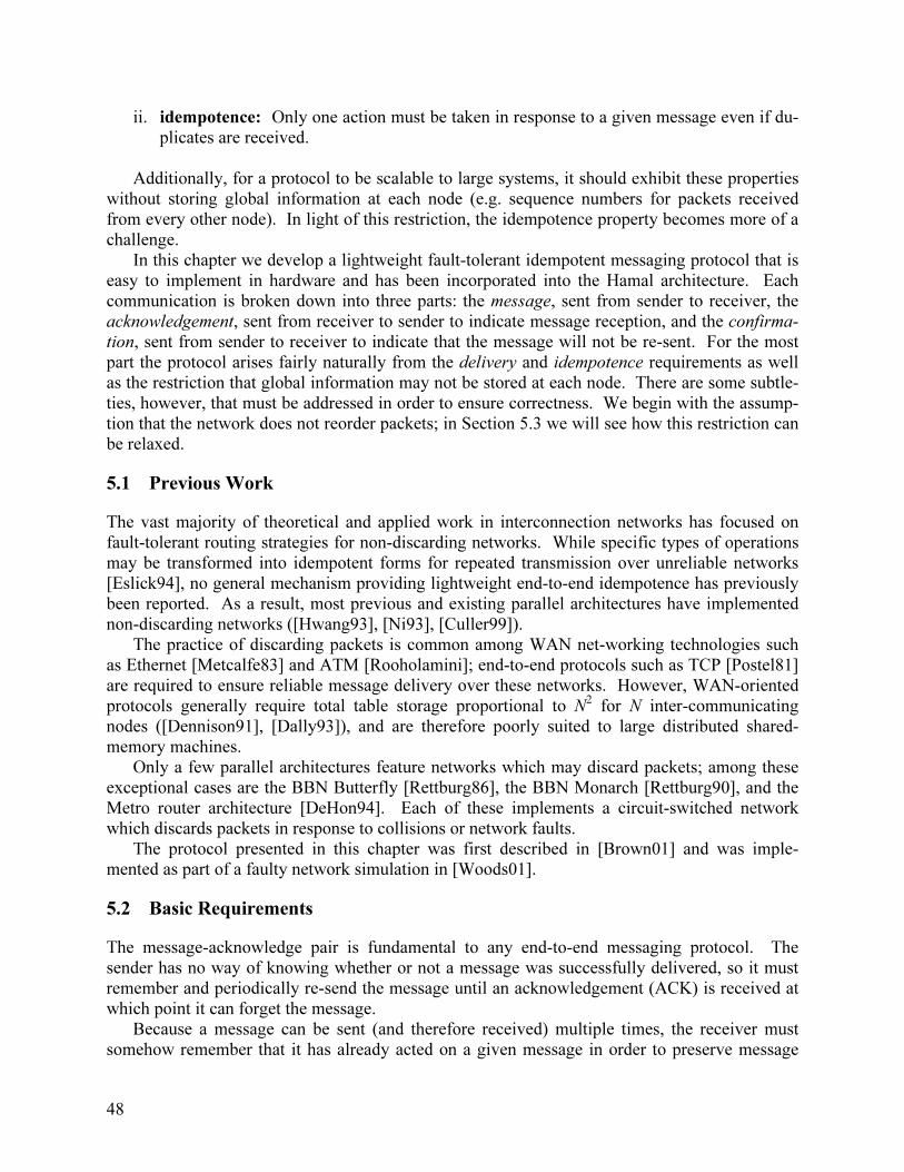
48

ii. idempotence: Only one action must be taken in response to a given message even if du-

plicates are received.

Additionally, for a protocol to be scalable to large systems, it should exhibit these properties

without storing global information at each node (e.g. sequence numbers for packets received

from every other node). In light of this restriction, the idempotence property becomes more of a

challenge.

In this chapter we develop a lightweight fault-tolerant idempotent messaging protocol that is

easy to implement in hardware and has been incorporated into the Hamal architecture. Each

communication is broken down into three parts: the message, sent from sender to receiver, the

acknowledgement, sent from receiver to sender to indicate message reception, and the confirma-

tion, sent from sender to receiver to indicate that the message will not be re-sent. For the most

part the protocol arises fairly naturally from the delivery and idempotence requirements as well

as the restriction that global information may not be stored at each node. There are some subtle-

ties, however, that must be addressed in order to ensure correctness. We begin with the assump-

tion that the network does not reorder packets; in Section 5.3 we will see how this restriction can

be relaxed.

5.1 Previous Work

The vast majority of theoretical and applied work in interconnection networks has focused on

fault-tolerant routing strategies for non-discarding networks. While specific types of operations

may be transformed into idempotent forms for repeated transmission over unreliable networks

[Eslick94], no general mechanism providing lightweight end-to-end idempotence has previously

been reported. As a result, most previous and existing parallel architectures have implemented

non-discarding networks ([Hwang93], [Ni93], [Culler99]).

The practice of discarding packets is common among WAN net-working technologies such

as Ethernet [Metcalfe83] and ATM [Rooholamini]; end-to-end protocols such as TCP [Postel81]

are required to ensure reliable message delivery over these networks. However, WAN-oriented

protocols generally require total table storage proportional to N2 for N inter-communicating

nodes ([Dennison91], [Dally93]), and are therefore poorly suited to large distributed shared-

memory machines.

Only a few parallel architectures feature networks which may discard packets; among these

exceptional cases are the BBN Butterfly [Rettburg86], the BBN Monarch [Rettburg90], and the

Metro router architecture [DeHon94]. Each of these implements a circuit-switched network

which discards packets in response to collisions or network faults.

The protocol presented in this chapter was first described in [Brown01] and was imple-

mented as part of a faulty network simulation in [Woods01].

5.2 Basic Requirements

The message-acknowledge pair is fundamental to any end-to-end messaging protocol. The

sender has no way of knowing whether or not a message was successfully delivered, so it must

remember and periodically re-send the message until an acknowledgement (ACK) is received at

which point it can forget the message.

Because a message can be sent (and therefore received) multiple times, the receiver must

somehow remember that it has already acted on a given message in order to preserve message

49

idempotence. One approach, used in the TCP protocol [Postel81], is to sequentially generate

packet numbers for every sender-receiver pair; each node then remembers the last packet number

that it received from every other node. This approach is feasible with thousands of nodes, but

the memory requirements are likely to be prohibitive in machines with millions of nodes.

Without maintaining this type of global information at each node, the only way to ensure

message idempotence is to remember individual messages that have been received. To ensure

correctness, each message must be remembered until a guarantee can be made that no more du-

plicates will be received. This, however, depends on a remote event, specifically the successful

delivery of an ACK to the sender. Only the sender knows when no more copies of the message

will be sent, and so we require a third confirmation (CONF) packet to communicate this informa-

tion to the receiver.

We thus have our three-part idempotent messaging protocol. The sender periodically sends a

message (MSG) until an ACK is received, at which point it can drop the message. Once a mes-

sage is received, the receiver ignores duplicates and periodically sends back an ACK until a

CONF is received, at which point it can forget about the message. Finally, each time that a

sender receives an ACK it responds with a CONF to indicate that the message will not be resent.

This is illustrated in Figure 5-1, which shows how the protocol is able to deal with arbitrary

packets being lost.

Figure 5-1: Idempotent messaging example.

MSG MSG

sender receiver

(a) Sender sends MSG and remembers it

MSG

MSG

MSG

ACK

(b) Receiver remembers MSG and sends ACK. Network

drops ACK. Sender re-sends MSG.

MSG MSGACK

(c) Receiver ignores duplicate message and re-sends ACK

MSG

CONF

ACK

(d) Sender forgets MSG and sends CONF. Network

drops CONF. Receiver sends third ACK.

CONF MSG

(e) Sender sends CONF in response to ACK

(f) Receiver receives CONF and forgets MSG

50

5.3 Out of Order Messages

The assumption that no more duplicate messages will be delivered once a CONF has been re-

ceived is true only if packets sent from one node to another are received in the order that they

were sent. If the network is permitted to reorder packets then the messaging protocol can fail as

shown in Figure 5-2.

This problem can be fixed as long as the amount of time allowed for a packet to traverse the

network is bounded. Suppose that all packets are either delivered or discarded at most T cycles

after they are sent. We modify the protocol by having the receiver remember a message for T

cycles after the CONF is received. Since any duplicate message would have been sent before the

CONF, by choice of T it is safe to forget the message after T cycles have elapsed.

We can ensure that the bound T exists either by assigning packets a time to live as in TCP

[Postel81], or by limiting both the number of cycles that a packet may be buffered by a single

network node and the length of the possible routing paths. The former approach places a tighter

bound on T, while latter is simpler as it does not require transmitting a time to live with each

packet.

Figure 5-2: Failure resulting from packet reordering.

5.4 Message Identification

Each message must be assigned an identifier (ID) that can be placed in the ACK and CONF

packets relating to that message. On the sending node the ID is sufficient to identify the mes-

sage; on the receiving node the message is uniquely identified by the pair (source node ID, mes-

sage ID). Figure 5-3 shows the structure of an ACK/CONF packet.

Figure 5-3: ACK/CONF packet structure.

A header field is present in all packets and contains the packet type and routing information.

The source node ID field identifies the node which sent the packet; for a CONF this is combined

with the message ID field at the receiving node to uniquely identify the message, and for an

MSG 7

sender receiver

(a) Sender resends message just before receiving ACK

MSG 7MSG 7

(b) Sender forgets MSG and sends CONF.

ACK 7

MSG 7

MSG 7

CONF 7

MSG 7MSG 7 CONF 7

(c) Network reorders MSG and CONF. Receiver forgets

MSG when it receives CONF, then idempotence is

lost when duplicate MSG is received.

header source node ID message ID

51

ACK it provides the destination for the CONF response (note that this information must be

stored in the ACK and cannot simply be remembered with the original message since the mes-

sage is discarded when the first ACK is received, but multiple ACKs may be received).

The ACK and CONF packets represent the overhead of the idempotent messaging protocol,

and as such it is desirable to make them as small as possible. It is tempting to try to use short

(say 4-8 bit) message ID’s and simply ensure that, on a given sending node, no two active mes-

sages have the same ID. Unfortunately, this approach fails because a message is “active” until

the CONF is received, and there is no way for the sending node to know when this occurs (short

of adding a fourth message to the protocol). Figure 5-4 shows how a message can be errone-

ously forgotten if message ID’s are reused too quickly.

Figure 5-4: Failure resulting from message ID reuse.

It is therefore necessary to use long message ID’s so that there is a sufficiently long period

between ID reuse. It is difficult to quantify “sufficiently long” since a message can, in theory, be

active for an arbitrarily long time if the network continually drops its CONF packets. One possi-

ble strategy is to use reasonably long ID’s, say 48 bits, then drain the network by suppressing

new messages once every 4-12 months of operation.

The next temptation is to eliminate the source node ID field and shorten the message ID field

in CONF packets only. This can be achieved by assigning to messages short secondary ID’s on

the receiving node so that CONF packets consist of only a header field and this secondary ID

(the source node ID is no longer necessary since the secondary ID’s are generated by the receiv-

ing node). Secondary ID’s can be direct indices into the receive table. However, the straight-

forward implementation of this idea also fails when secondary ID’s are reused prematurely.

Figure 5-5 shows how a message can lose its idempotence when this occurs.

Fortunately, a more careful implementation of secondary ID’s does, in fact, work. The key

observation is that because the sending node forgets CONF packets as soon as they are sent, we

can place a bound on the amount of time that a secondary ID remains active after a CONF has

MSG 7

sender receiver

(a) Receiver sends ACK to message with ID = 7

MSG 7

CONF 7

ACK 7

(b) Sender forgets MSG and sends CONF. Network

drops CONF. Receiver re-sends ACK.

ACK 7 MSG 7

MSG 7

MSG 7

ACK 7

(c) While ACK is in transit, sender re-uses ID 7 for a new

message which is dropped by the network.

MSG 7

CONF 7 MSG 7

(d) Sender receives ACK and forgets the new message,

thinking it has been received.

52

been received. If an ACK was sent before the CONF was received, then the secondary ID will

be active as long as the ACK is traveling to the sender, or the sender is processing the ACK, or

the CONF response is traveling back to the receiver. We have already seen how to place a

bound T on packet travel time. If in addition we place a bound R on the time taken to process an

ACK (dropping the packet if it cannot be serviced in time), then a secondary ID can remain ac-

tive for at most 2T + R cycles after the first CONF is received. We can therefore avoid secon-

dary ID reuse by remembering a message for 2T + R cycles after the CONF is received.

Figure 5-5: Failure resulting from secondary ID reuse.

5.5 Hardware Requirements

In addition to the control logic needed to implement the protocol, the primary hardware require-

ments are two content addressable memories (CAMs) used for remembering messages. The first

of these remembers messages sent, stores {message ID, message index} on each line, and is ad-

dressed by message ID. “message index” locates the actual message and is used to free re-

sources when an ACK is received. The processor is prohibited from generating new messages if

this send table fills, and must stall if it attempts to do so until an entry becomes available. The

second CAM remembers messages received, stores {source node ID, message ID} on each line

and is addressed by (source node ID, message ID). No additional information is required in this

CAM since the receiver simply needs to know whether or not a particular message has already

been received. If this table is full, new messages received over the network are dropped.

MSG 5

sender receiver

(a) Sender sends message with ID = 5

(b) Receiver assigns secondary ID = 2 and responds with

ACK containing both primary and secondary ID

MSG 5

MSG 9

(c) Sender forgets MSG, sends CONF and a new MSG.

Meanwhile, receiver re-sends ACK.

MSG 9

CONF 2

(d) Receiver forgets MSG 5, reuses secondary ID 2 for

MSG 9, and sends ACK which is dropped by the net-

work. Sender responds to second ACK with CONF.

MSG 5,2MSG 5 ACK 5,2

CONF 2

MSG 5,2

ACK 5,2

MSG 9 MSG 9,2

ACK 9,2

MSG 9 MSG 9

(e) Receiver receives CONF and forgets MSG 9, thinking

that it will not be resent. Meanwhile, sender does re-

send MSG 9, and idempotence is lost.

53

Chapter 6

The Hamal Microkernel

I claim not to have controlled events, but confess plainly that events have controlled me.

– Abraham Lincoln (1809-1865), in a letter to Albert G. Hodges

The resources of the Hamal processor-memory node are managed by a lightweight event-driven

microkernel that runs concurrently in context 0. This approach has the effect of blurring the dis-

tinction between hardware and software, and necessitates an integrated design methodology. In-

deed, throughout the course of the design process, many hardware mechanisms have been re-

placed by software alternatives, and many basic kernel tasks have been migrated into hardware.

The resulting design reflects an effort to maximize system efficiency and flexibility while keep-

ing both the hardware and the kernel as simple as possible. In this chapter we describe the vari-

ous aspects of the Hamal microkernel, including both its event handling strategies and the inter-

face it presents to user applications.

6.1 Page Management

The Hamal instruction set contains privileged instructions that allow the kernel to create, destroy,

page in and page out pages of memory. All page management instructions take a virtual page

address as their operand. The kernel is never required (or able) to manipulate physical page

numbers; it is simply required to keep track of the number of free pages in each bank.

The use of capabilites guarantees that a page fault is always caused by an attempt to access a

page which is not resident in memory and is never due to a program error. This fact, together

with the use of virtual addresses to reference pages both in memory and in secondary storage,

means that there is no need for the kernel to maintain any sort of page tables.

There are two types of page fault events: data page faults, caused by memory references, and

code page faults, caused by instruction fetching. The kernel handles both types of events by is-

suing a page-in request and writing the event information to a page-in table in memory, so that

the faulting operation may be resumed when the page arrives. For a data page fault, this infor-

mation consists of the memory operation, the memory address, the reply address, up to 128 bits

of data, and a trap vector. For a code page fault, the information consists of the instruction ad-

dress and the swap address of the faulting thread. In the case of a code page fault the kernel also

suspends the offending thread.

Secondary storage responds to page-in requests by using the virtual address to physically lo-

cate the page; it then fetches the page and sends it to the requesting node. If the page does not

exist, which occurs the first time a new data page is accessed, it is created and initialized with

zeros. When a code or data page-in completes, a page-in event is generated which supplies the

54

kernel with the virtual address of the newly arrived page. The kernel searches the page-in table

for matching data page fault entries, and uses a special privileged instruction to reissue memory

requests (this must be done even for code memory page-ins because code is readable). If the

new page is a code page, the kernel also searches the table for matching code page fault entries,

reactivating the corresponding threads.

6.2 Thread Management

Privileged mode instructions allow the kernel to suspend, resume, and terminate threads. As

with the page management instructions, these instructions all take the virtual swap address of a

thread as their operand. The kernel is neither required nor able to manipulate physical context

numbers, but must keep track of the number of free contexts.

The kernel maintains threads in four doubly linked lists according to their state. active

threads are those currently executing in one of the hardware contexts. new threads have been

created to handle a trap or in response to a fork event but have not yet been activated. ready

threads have been swapped out to allow other threads to run, and are ready to continue execution

at any time. suspended threads are blocked, and are waiting for a memory reply, a code page, or

a join operation.

When a fork is added to a node’s hardware fork queue a fork event is generated. When the

kernel handles this event, it allocates a new swap page by advancing a counter and creating the

page. If there is a free context, the kernel loads the new thread immediately and places it in the

‘active’ list. Otherwise, it writes the thread to the swap page and adds it to the ‘new’ list. To

improve the efficiency of micro-threads that perform a very simple task and then exit, the kernel

attempts to reserve a context for new threads. This allows these threads to run immediately

without having to wait for a longer-running thread to relinquish a context.

When a stall event occurs (Section 4.3.2), the kernel checks to see if there are any new or

ready threads waiting to execute. If so, the stalled thread is suspended. Otherwise, the stall

event is ignored. If the thread is suspended, it is not immediately added to the ‘suspend’ list; the

kernel simply issues the suspend instruction and returns to the head of the event loop. This al-

lows other events to be processed while the thread state dribbles back to its swap page. Once the

thread has been completely unloaded, a suspend event is generated to inform the kernel that the

contents of the swap page are valid and that the context is available. At this point the kernel adds

the thread to the ‘suspend’ list and checks to see if it can activate any new or ready threads.

In addition to the suspend event which is generated after a thread has been manually sus-

pended, there are four other events which indicate to the kernel that a thread is unable to continue

execution. A code page fault event occurs when a thread tries to execute an instruction group

located in a non-resident page, and was described in the previous section. A code T trap event

occurs when a thread tries to execute an instruction group with the T trap bit set. A break event

occurs when a thread issues a break instruction; this is the normal mechanism for thread termina-

tion. The kernel responds to a break event by removing the thread from the ‘active’ list and

checking to see if it can activate any new or ready threads. A trap event occurs when a thread

encounters an error condition and its trap vector is invalid. Each of these events is placed in the

event queue after the faulting thread has been dribbled to memory, so the kernel can assume that

the contents of the swap page are valid and the thread’s context is available.

When a reply to a memory request is received, the processor checks to see if the requesting

thread is still active in one of the contexts. If so, the reply is processed by that context. Other-

wise a reply event is generated. The kernel handles this event by directly modifying the contents

55

of the thread’s swap page. If the thread was suspended and the kernel determines that the reply

will allow the thread to continue executing, then the thread is reactivated if there is more than

one free context (recall that one context is reserved for new threads), otherwise it is moved to the

‘ready’ list.

Thread scheduling is performed using a special purpose count-down register which is decre-

mented every cycle when positive and which generates a timer event when it reaches zero. If

there are no threads waiting to be scheduled, then the timer event is simply ignored. Otherwise

the least recently activated thread (i.e. the thread at the head of the ‘active’ list) is suspended us-

ing the suspend instruction.

6.3 Sparsely Faceted Arrays

In order to support sparsely faceted arrays, the kernel must supply the network interface with

translations when translation cache misses occur. Two events notify the kernel of cache misses:

translate-in events, generated by failed global→local translations, and translate-out events, gen-

erated by failed local→global translations. The kernel maintains a full translation table, and re-

sponds to translation events by looking up the appropriate translation and communicating it to

the network interface using the privileged xlate instruction. If no translation is found, which can

only occur for a translate-in event the first time a node encounters an xsparse capability for a

SFA, the kernel uses the segment size information embedded in the xsparse capability to allocate

a local facet, and the base address of this facet is entered into the translation table.

6.4 Kernel Calls

The kernel exposes a set of privileged subroutines to user applications by creating a kernel table

of entry points in memory, then placing a read-only capability for this table in one of the shared

registers. The entry points are all code capabilities with the P (execute privileged), I (increment

only) and D (decrement only) bits set, allowing applications to call these subroutines in privi-

leged mode. Table 6-1 lists some examples of kernel subroutines.

Subroutine Description

trap Default trap handler

malloc Allocate a data capability

smalloc Allocate a sparse capability

xmalloc Allocate an xsparse capability

fopen Open an existing file

fnew Create a file

Table 6-1: Kernel subroutines examples.

Because the trap and malloc entry points are used so frequently (threads typically copy trap

into the trap vector when they initialize, and malloc is called to allocate memory), they are stored

in shared registers so that they may be accessed directly. The fopen and fnew routines return IO

capabilities that allow applications to communicate with the external host.

The malloc routine allocates memory simply by advancing an allocation counter. The alloca-

tion counter is stored in a shared register. Spin-wait synchronization is used to obtain the

counter; malloc begins by atomically reading and resetting the shared register (using two instruc-

56

tions in a single instruction group) until a non-zero value is read. After the memory is allocated

the counter is advanced and written back into the shared register. Both malloc and xmalloc use

the same counter; smalloc uses a separate counter so that multiple sparse objects allocated by the

same node will be stored contiguously on all nodes.

6.5 Forwarding Pointers

Hamal implements forwarding pointers by setting the T trap bit of a 128-bit memory word and

storing the forwarding pointer in that word. When a memory request attempts to access a for-

warding pointer, the memory system attempts to automatically forward the request. In some

cases, however, it may not be possible for the request to forwarded in hardware (see Chapter 7:

Deadlock Avoidance). In these cases a data T trap event is generated. The kernel spawns a new

thread to handle the trap and forward the memory request. When this thread runs, it uses the

loadw instruction, a privileged non-trapping load, to read the forwarding pointer from memory,

and then reissues the memory request using the new address.

The default trap handler supplied by the kernel contains code to handle squid traps, caused by

pointer comparison instructions that cannot be completed in hardware, as described in Section

3.2.2. The handler uses loadt, a privileged instruction to inspect a T trap bit, in conjunction with

loadw to determine the final addresses of the pointers being compared. It then performs the

comparison and manually updates the predicate register specified as the destination of the trap-

ping instruction.

6.6 UV Traps

When a memory reference causes a U/V trap (Section 3.3.5), a UV trap event is generated. The

kernel responds to this event by creating a new thread to handle the event. The starting address

for this thread is the user-supplied trap vector which accompanies every potentially-trapping

memory request. The thread is created in memory, and is initialized with the UV trap informa-

tion. It is activated immediately if a context is available, otherwise it is added to the ‘new’ list.

The kernel must create this thread manually and cannot simply issue a fork as this is a potentially

blocking instruction (see Chapter 7).

6.7 Boot Sequence

The boot sequence on a processing node is initiated by the arrival of a page of code whose virtual

address is zero, at which point context 0 starts executing the code from the beginning. This page

contains the start of the kernel loader which performs the following tasks in order:

1. Root code and data capabilities are created.

2. The rest of the kernel code pages are paged in from secondary storage.

3. Kernel data pages are created and initialized

4. The kernel table is created and the shared registers are initialized.

5. The code pages containing the kernel loader are destroyed.

6. The kernel loader branches to the head of the event loop.

At this point the event queue will be empty and the kernel will stall waiting for an event. The

external host can then initiate user applications by injecting one or more fork messages into the

machine.

57

Chapter 7

Deadlock Avoidance

Advance, and never halt, for advancing is perfection.

– Kahlil Gibran (1883-1931), “The Visit of Wisdom”

One of the most important considerations in designing a large parallel system is ensuring that it

is deadlock-free. Much of the literature regarding deadlock avoidance deals exclusively with the

network, which is the most obvious potential source of deadlocking problems. In a non-

discarding network, one must rely on either topological routing constraints [Dally87] or virtual

channels [Dally93] to prevent network deadlock. In addition, it is necessary to guarantee that

nodes can always sink packets that arrive over the network. A discarding network, by contrast,

finesses the problem by simply dropping packets that cannot make forward progress. As a result,

cyclic routing dependencies are transient at worse and will never bring the machine to a halt.

There are, however, two other potential sources of deadlock in the system. The first of these is

inter-node deadlock, caused by a group of nodes that exhaust their network resources while try-

ing to send each other packets. Consider the simple case in which programs running on two dif-

ferent nodes issue a large number of remote read requests to each other’s memory (Figure 7-1).

If the send and receive tables on each node should fill up with these requests, then no more for-

ward progress will be made. No packets can be delivered because the receive tables are full, and

no packets can be processed because the send tables are full so there is no room for the read re-

plies. The second possible type of deadlock is intra-node deadlock, which occurs when the

event-handling microkernel becomes wedged. This can happen, for example, if the kernel issues

a read request which causes a page fault. A page fault event will be placed on the event queue

but will never be serviced; the kernel thread will stall indefinitely waiting for the read operation

to complete.

Figure 7-1: Inter-node deadlock can occur if the network tables fill up.

processor

memory

processor

memory

58

Eliminating these potential sources of deadlock requires cooperation between the hardware

design and the software microkernel. In this chapter we outline the strategies used in the Hamal

architecture and microkernel to ensure that the entire system is provably deadlock-free.

7.1 Hardware Queues and Tables

To first order approximation, the possibility of deadlock emerges directly from the presence of

hardware queues and tables. A hardware queue/table has a fixed size and can potentially fill up;

when it does backpressure must be exerted to suppress various other events and operations. We

therefore begin our discussion of deadlock avoidance by reviewing the hardware queues and ta-

bles of the Hamal processor-memory nodes and the various types of backpressure used to ensure

that they do not overflow.

As shown in Figure 7-2, there are two queues and two tables that need to be considered. First

and foremost is the hardware event queue. Events can be generated by the processor (e.g. thread

termination, memory replies), the memory banks (e.g. page faults, memory traps), or the network

interface (e.g. translation cache miss, forks). The second queue is the fork queue which is fed by

both the network interface and the local processor. Finally, the network interface contains two

tables: a send table, fed by the processor and the memory banks (for replies to remote memory

operations or forwarded addresses), and a receive table, which is fed by the network.

Figure 7-2: Hardware queues and tables in the Hamal processor-memory node.

If the receive table fills, no packets will be accepted from the network. If the fork queue fills,

fork packets in the receive table will not be processed, and any context that tries to issue a fork

instruction will stall. Having the send table or event queue fill is a much more serious problem

as in this case a memory bank could stall if it needs to generate an event or service a remote

memory request. This in turn can deadlock the node if the kernel needs to access the stalled

memory bank to make forward progress. Mechanisms are therefore required to ensure that mem-

ory banks are always able to finish processing requests.

ev

en

ts

send

receive

network

interface

memory

processor

fork

s

59

The node controller guarantees space in the send table by reserving entries in advance. Be-

fore accepting a remote memory request from the network or a local request from the processor

with a remote return address, the controller attempts to reserve a spot in the send table. If it is

unable to do so then the memory request is blocked. If a remote memory request is allowed to

proceed to the appropriate memory bank but causes a trap, an event is added to the event queue

and the send table reservation for that request is cancelled.

The event queue is prevented from overflowing using a high water level mechanism. If the

event queue fills beyond the high water level, all operations which can potentially give rise to

new events are throttled. Other potentially event-causing operations may already be in progress;

the high water level mark is chosen so that there are enough free entries to accept these events.

Network events are suppressed, and no forks, joins or memory requests are accepted from the

network. Processor events (such as thread termination) are suppressed. All memory requests are

blocked except for those generated by context 0. Once the kernel has processed enough events

to bring the event queue below the high water level, normal operation resumes.

7.2 Intra-Node Deadlock Avoidance

We begin by describing a set of requirements to prevent an individual node from deadlocking.

In the following section we show how to use the assumption that individual nodes are deadlock-

free to avoid inter-node deadlocks. For now, however, we can make no assumptions about the

system as a whole, and in particular we must allow for the possibility that packets destined to

other nodes remain in the send table for arbitrarily long periods of time.

To avoid intra-node deadlock, we must be able to guarantee that the microkernel’s event han-

dling routines do not block and finish executing in a finite amount of time. This ensures that

forward progress can always be made, independent of the pattern of events which occur. For the

most part this is easy to do; software exceptions can be avoided through careful programming,

and instructions requiring machine resources that may not be available (e.g. fork) can be avoided

altogether. The difficulty lies in performing memory operations, since every memory reference

can potentially generate a page fault or a trap.

The solution to this problem requires cooperation between the kernel and the hardware. The

kernel must not issue a potentially trapping memory request, a remote memory request, or a

memory request with a remote return address. When the kernel accesses local memory it must

ensure that the page being referenced is present in memory. If a page is not present, then the

kernel must first page it in and spin-wait for it to arrive, possibly first paging out another page to

make room. Thus, the hardware must guarantee that page-ins and page-outs can always com-

plete without blocking.

Figure 7-3 shows the complete path taken by a page-in request; page-outs follow the first half

of this path. We can ensure that secondary storage requests do not block by working backwards

along this path. First, the processor-memory node must be able to process the page-in packet.

Processing a page-in usually involves storing the page to memory and generating a page-in

event. However, this can cause problems if the kernel needs to page-in and spin-wait for several

pages; the resulting page-in events could overwhelm the event queue. We avoid this situation

with a special version of the pagein instruction that does not generate an event when the page is

loaded. By using this instruction to load pages that are needed immediately, the kernel guaran-

tees that the node will be able to process the page when it arrives.

60

Figure 7-3: Life cycle of a page-in request.

Next, the network interface must be able to receive the page-in packet sent from secondary

storage. This is guaranteed by reserving an entry in the network receive table for secondary stor-

age packets. If a packet arrives from some other source and there is only one available receive

table entry, that packet is dropped. Moving backwards along the path, secondary storage simply

handles requests in the order that they are received and will never block. Although its send table

can potentially fill up, the fact that nodes can always eventually receive secondary storage pack-

ets implies that a send table entry will become available in a finite amount of time. Finally, a

node must always be able send page-in and page-out packets to secondary storage. We again

make this guarantee by reserving a table entry for secondary storage packets, this time in the

send table. The combination of an event-free pagein instruction and reserved entries in the send

and receive tables ensures that page-in and page-out operations can always proceed to comple-

tion. This in turn implies that the event-handling microkernel can always make forward pro-

gress, so the nodes are deadlock-free.

There is still one subtlety that must be addressed with regard to page-ins. While the above

mechanisms are sufficient to ensure that event-free page-ins will never become blocked, we must

also consider those page-ins which are issued in response to a page fault and which must be al-

lowed to generate an event when they arrive at the node. Furthermore, at any given time there

could be many active page-in requests at various points in the path of Figure 7-3. The event

queue must be able to absorb their events when they arrive at the node: the page-ins cannot stall

in the receive table until an event queue slot becomes available as this could block a page-in for

which the kernel is spin-waiting, nor can the reserved receive table entry be designated for event-

free page-ins only as then the secondary storage send table could fill with event-generating page-

ins that cannot be sent. One solution is to lower the event-queue high water mark to allow for

some specified number of in-flight page-ins, requiring that the kernel cooperate by never request-

ing more than that number of page-ins simultaneously. A slightly more efficient solution, im-

plemented in the Hamal architecture, is to maintain a separate event queue specifically for page-

in events. This avoids wasting large event-queue entries (512 bits each) for small page-in events

(each page-in event simply consists of the virtual base address of the newly arrived page).

Again, the kernel cooperates by restricting the number of simultaneously requested pages.

7.3 Inter-Node Deadlock Avoidance

We can now use the fact that individual nodes are deadlock-free to eliminate the possibility of

inter-node deadlocks. A sufficient condition for the system to be deadlock free is for every re-

quest in a node’s network receive table entry to be processed in a finite amount of time. The dif-

ficulty is that some of these requests cannot be processed unless there is space in the send table;

it is this dependency that leads to the deadlock situation illustrated in Figure 7-1. We will refer

page

fetch page

node secondary storage

page-in

61

to these as non-terminal requests. A terminal request is one that can be processed by the node

without generating a new remotely destined request. Terminal requests consist of forks, joins

(Section 4.4) and replies to remote memory references. Non-terminal requests consist of all

memory operations. We can leverage the fact that, because a given node is deadlock-free, all

terminal requests in the receive table will eventually be processed by the node.

The network send and receive tables already have an entry reserved for secondary storage

packets. Our approach to inter-node deadlock avoidance is to reserve an additional entry in each

table for terminal requests. We claim that with this simple hardware modification, the system as

a whole is deadlock-free. To see this, suppose that a node is unable to process one of the packets

in its receive table. This implies both that the packet is a non-terminal request (i.e. a remote

memory request) and that a reservation cannot be made in the send table for the reply to this re-

quest. Since a memory reply is a terminal request, this means that the terminal request entry in

the send table is occupied. But this terminal request will eventually be delivered to its destina-

tion, because the destination node has a receive entry reserved for terminal requests. It doesn’t

matter if this entry is occupied or if there are other nodes competing for it; because the destina-

tion node can always service terminal requests, with probability 1 the terminal request will even-

tually be successfully delivered. Thus, the terminal request entry in the send table will eventu-

ally be unoccupied, allowing the remote memory request to be processed. Again, it doesn’t mat-

ter if other non-terminal requests, existing in the receive table or locally generated, are compet-

ing for the send table; as long as the node’s arbitration policy is starvation-free, with probability

1 the memory request will eventually be processed by the node.

What makes this approach possible is the fact that when a non-terminal request is serviced, a

terminal request is generated. There is, however, one exception to this rule: if a request encoun-

ters a forwarding pointer, it is automatically forwarded, possibly generating a new non-terminal

request if the forwarding destination is remote. This is not a problem, and does not affect the

above proof, so long as the send table reservation for that request was not made using the entry

set aside for terminal requests. If it was, then the request cannot be automatically forwarded.

Instead, the node controller cancels the send table reservation and generates a data T trap event

to be handled by the microkernel.

62

63

Part II – Evaluation

There is nothing either good or bad, but thinking makes it so.

– William Shakespeare (1564-1616), “Hamlet”, Act 2 scene 2

It is a capital mistake to theorize before one has data.

– Sir Arthur Conan Doyle (1859-1930), “Scandal in Bohemia”

64

65

Chapter 8

Simulation

I just bought a Mac to help me design the next Cray.

– Seymour Cray (1925-1996)

Our evaluations of the Hamal parallel architecture are based on a cycle accurate simulator of the entire system. In this chapter we describe our simulation methodology. We begin by presenting Sim, a C++ framework for cycle-based simulation that was developed to facilitate the construc-tion of the Hamal simulator. We then give an overview of the Hamal simulator, and we describe the development environment used to edit, assemble, run and debug both the kernel and bench-mark applications.

8.1 An Efficient C++ Framework for Cycle-Based Simulation

Software simulation is a critical step in the hardware design process. Hardware description lan-guages such as Verilog and VHDL allow designers to accurately model and test the target hard-ware, and they provide a design path from simulation to fabrication. However, they are also no-toriously slow, and as such are not ideal for simulating long runs of a large, complex system. Instead, a high-level language (usually C or C++) is generally used for initial functional simula-tions. Inevitably, the transition from this high-level simulation to a low-level hardware descrip-tion language is a source of errors and increased design time.

Recently there have been a number of efforts to develop simulation frameworks that enable the accurate description of hardware systems using existing or modified general-purpose lan-guages ([Ku90], [Liao97], [Gajski00], [Ramanathan00], [Cyn01], [SC01]). This bridges the gap between high-level and register transfer level simulations, allowing designers to progressively refine various components within a single code base. The approach has been successful: one group reported using such a framework to design a 100 million transistor 3D graphics processor from start to finish in two months [Kogel01].

There are four important criteria to consider when choosing or developing a framework:

Speed: The simulator must be fast. Complex simulations can take hours or days; a faster simulator translates directly into reduced design time.

Modularity: There should be a clean separation and a well-defined interface between the vari-

ous components of the system.

66

Ease of Use: The framework should not be a burden to the programmer. The programming interface should be intuitive, and the framework should be transparent wherever possible.

Debugging: The framework must contain mechanisms to aid the programmer in detecting er-

rors within the component hierarchy. These criteria were used to create Sim, a cycle-based C++ simulation framework used to

simulate the Hamal architecture. Through experience we found that Sim met all four criteria with a great deal of success. In the following sections we describe the Sim framework and we report on what we observed to be its most useful features. We also contrast Sim with SystemC [SC01], an open-source C++ simulation framework supported by a number of companies.

8.1.1 The Sim Framework

To a large extent, the goals of speed and modularity can be met simply by choosing an efficient object-oriented language, i.e. C++. What distinguishes a framework is its simulation model, programming interface and debugging features. Sim implements a pure cycle-based model; time is measured in clock ticks, and the entire system exists within a single clock domain. The pro-grammer is provided with three abstractions: components, nodes and registers. A component is a C++ class which is used to model a hardware component. In debug builds, Sim automatically generates hierarchical names for the components so that error messages can give the precise lo-cation of faults in the simulated hardware. A node is a container for a value which supports con-nections and, in debug builds, timestamping. Nodes are used for all component inputs and out-puts. Registers are essentially D flip-flops. They contain two nodes, D and Q; on the rising clock edge D is copied to Q.

Simulation proceeds in three phases. In the construction phase, all components are con-structed and all connections between inputs and outputs are established. When an input/output node in one component is connected to an input/output node in another component, the two nodes become synonyms, and writes to one are immediately visible to reads from the other. In the initialization phase, Sim prepares internal state for the simulation and initial values may be assigned to component outputs. Finally, the simulation phase consists of alternating calls to the top-level component’s Update function (to simulate combinational evaluation) and a global Tick function (which simulates a rising clock edge).

Figure 8-1 gives an example of a simple piece of hardware that computes Fibonacci numbers and its equivalent description using Sim. The example shows how components can contain sub-components (Fibonacci contains a ClockedAdder), how nodes and registers are connected during the construction phase (using the overloaded left shift operator), and how the simulation is run at the top level via alternating calls to fib.Update() and Sim::Tick(). The component functions Construct() and Init() are called automatically by the framework; Update() is called explicitly by the programmer.

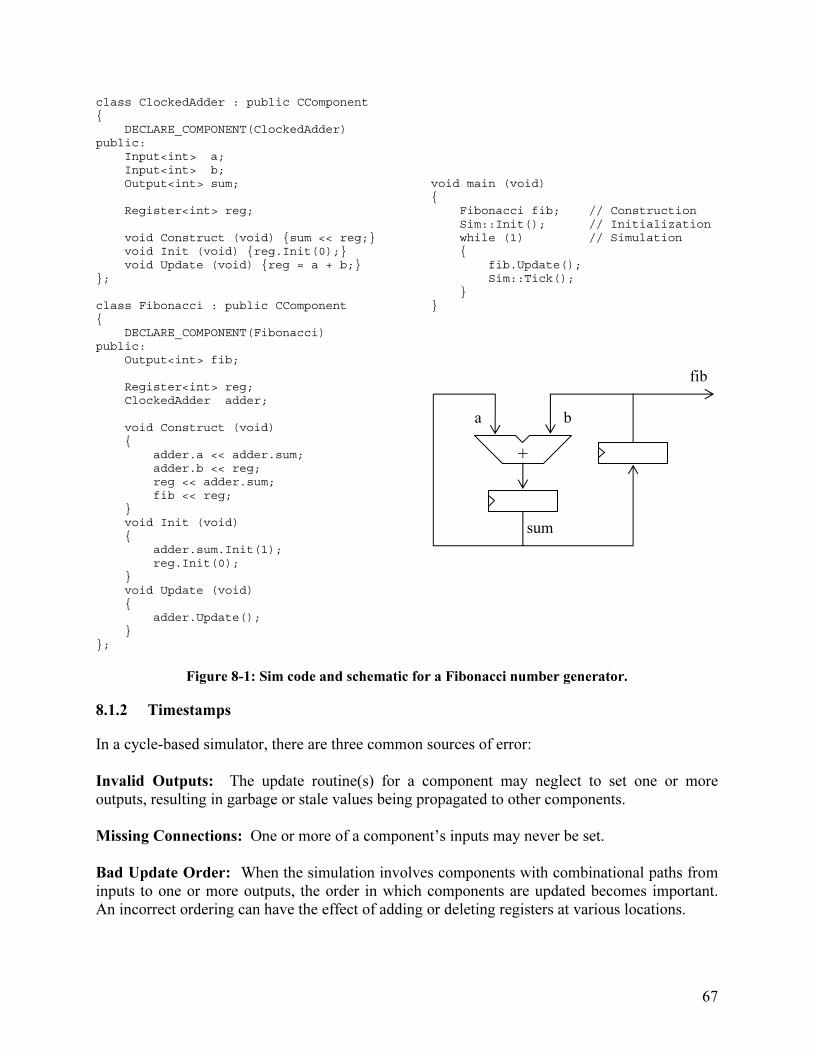
67

class ClockedAdder : public CComponent{

DECLARE_COMPONENT(ClockedAdder)public:

Input<int> a;Input<int> b;Output<int> sum;

Register<int> reg;

void Construct (void) {sum << reg;}void Init (void) {reg.Init(0);}void Update (void) {reg = a + b;}

};

class Fibonacci : public CComponent{

DECLARE_COMPONENT(Fibonacci)public:

Output<int> fib;

Register<int> reg;ClockedAdder adder;

void Construct (void){

adder.a << adder.sum;adder.b << reg;reg << adder.sum;fib << reg;

}void Init (void){

adder.sum.Init(1);reg.Init(0);

}void Update (void){

adder.Update();}

};

void main (void){

Fibonacci fib; // ConstructionSim::Init(); // Initializationwhile (1) // Simulation{

fib.Update();Sim::Tick();

}}

Figure 8-1: Sim code and schematic for a Fibonacci number generator.

8.1.2 Timestamps

In a cycle-based simulator, there are three common sources of error:

Invalid Outputs: The update routine(s) for a component may neglect to set one or more outputs, resulting in garbage or stale values being propagated to other components.

Missing Connections: One or more of a component’s inputs may never be set.

Bad Update Order: When the simulation involves components with combinational paths from inputs to one or more outputs, the order in which components are updated becomes important. An incorrect ordering can have the effect of adding or deleting registers at various locations.

a b

sum

fib

+

68

While careful coding can avoid these errors in many cases, experience has shown that it is generally impossible to write a large piece of software without introducing bugs. In addition, these errors are particularly difficult to track down as in most cases they produce silent failures which go unnoticed until some unrelated output value is observed to be incorrect. The pro-grammer is often required to spend enormous amounts of time finding the exact location and na-ture of the problem.

The Sim framework helps the programmer to eliminate all three sources of error by time-stamping inputs and outputs. In debug builds, each time a node is written to it is timestamped, and each time a node is read the timestamp is checked to ensure that the node contains valid data. When an invalid timestamp is encountered, a warning message is printed which includes the automatically generated name of the input/output, pinpointing the error within the component hierarchy.

Timestamped nodes have proven to be by far the most useful feature of the Sim framework. They can speed up the debugging process by an order of magnitude, allowing the programmer to detect and correct errors in minutes that would otherwise require hours of tedious work. Figure 8-2 shows the exact warning message that would be generated if the connection “adder.b << reg” were omitted from the function Fibonacci::Construct() in Figure 8-1.

Warning: Fibonacci0::Adder0::Input1

Invalid timestampc:\projects\sim\sim.h, line 527, simTime = 1

Figure 8-2: Warning message generated if the programmer forgets the connection adder.b << reg.

8.1.3 Other Debugging Features

The Sim framework provides a number of Assert macros which generate warnings and errors. As is the case with standard assert macros, they give the file and line number at which the error condition was detected. In addition, the error message contains the simulation time and a precise location within the component hierarchy (as shown in Figure 8-2). Again, this allows the pro-grammer to quickly determine which instance of a given component was the source of the error.

When one node A is connected to another node B, the intention is usually to read from A and write to B (note that order is important; connecting A to B is not the same as connecting B to A). Timestamps can be used to detect reads from B, but not writes to A. To detect this type of error, in debug builds a node connected to another node is marked as read-only1; assignment to a read-only node generates a warning message. In practice this feature did not turn out to be very useful as the simple naming convention of prefixing inputs with in_ and outputs with out_ tended to prevent these errors. The feature does, however, provide a safety net, and it does not affect re-lease builds of the simulator.

8.1.4 Performance Evaluation

Making use of a simulation framework comes at a cost, both in terms of execution time and memory requirements. We can quantify these costs for the Sim framework by implementing four low-level benchmark circuits in both Sim and straight C++. The most important difference between the implementations is that inputs and outputs in the C++ versions are ordinary class

1 Unless the node has been declared as a bi-directional Input/Output.

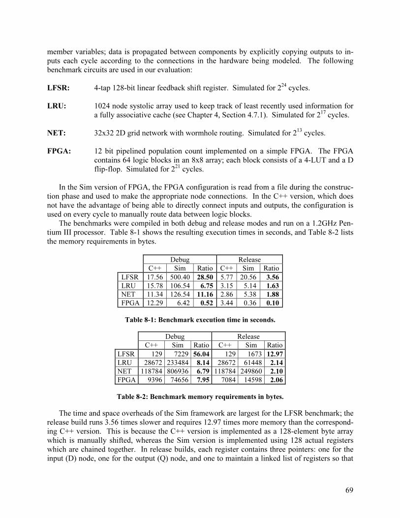
69

member variables; data is propagated between components by explicitly copying outputs to in-puts each cycle according to the connections in the hardware being modeled. The following benchmark circuits are used in our evaluation:

LFSR: 4-tap 128-bit linear feedback shift register. Simulated for 224 cycles.

LRU: 1024 node systolic array used to keep track of least recently used information for

a fully associative cache (see Chapter 4, Section 4.7.1). Simulated for 217 cycles.

NET: 32x32 2D grid network with wormhole routing. Simulated for 213 cycles.

FPGA: 12 bit pipelined population count implemented on a simple FPGA. The FPGA contains 64 logic blocks in an 8x8 array; each block consists of a 4-LUT and a D flip-flop. Simulated for 221 cycles.

In the Sim version of FPGA, the FPGA configuration is read from a file during the construc-

tion phase and used to make the appropriate node connections. In the C++ version, which does not have the advantage of being able to directly connect inputs and outputs, the configuration is used on every cycle to manually route data between logic blocks.

The benchmarks were compiled in both debug and release modes and run on a 1.2GHz Pen-tium III processor. Table 8-1 shows the resulting execution times in seconds, and Table 8-2 lists the memory requirements in bytes.

Debug Release

C++ Sim Ratio C++ Sim Ratio

LFSR 17.56 500.40 28.50 5.77 20.56 3.56

LRU 15.78 106.54 6.75 3.15 5.14 1.63

NET 11.34 126.54 11.16 2.86 5.38 1.88

FPGA 12.29 6.42 0.52 3.44 0.36 0.10

Table 8-1: Benchmark execution time in seconds.

Debug Release

C++ Sim Ratio C++ Sim Ratio

LFSR 129 7229 56.04 129 1673 12.97

LRU 28672 233484 8.14 28672 61448 2.14

NET 118784 806936 6.79 118784 249860 2.10

FPGA 9396 74656 7.95 7084 14598 2.06

Table 8-2: Benchmark memory requirements in bytes.

The time and space overheads of the Sim framework are largest for the LFSR benchmark; the release build runs 3.56 times slower and requires 12.97 times more memory than the correspond-ing C++ version. This is because the C++ version is implemented as a 128-element byte array which is manually shifted, whereas the Sim version is implemented using 128 actual registers which are chained together. In release builds, each register contains three pointers: one for the input (D) node, one for the output (Q) node, and one to maintain a linked list of registers so that

70

they can be automatically updated by the framework when Sim::Tick() is called. This, together with the 129 bytes of storage required for the actual node values, accounts for the factor of 13 increase in memory usage. Clearly the register abstraction, while more faithful to the hardware being modeled, is a source of inefficiency when used excessively.

The execution time and memory requirements for the release builds of the other three Sim benchmarks compare more favorably to their plain C++ counterparts. In all cases the memory requirements are roughly doubled, and the worst slowdown is by a factor of 1.88 in NET. In the FPGA benchmark the Sim implementation is actually faster by an order of magnitude. This is due to the fact that the framework is able to directly connect nodes at construction time as di-rected by the configuration file.

Not surprisingly, the Sim framework overhead in the debug builds is quite significant. The debug versions run roughly 20-25 times slower than their release counterparts, and require four times as much memory. This is largely a result of the node timestamping that is implemented in debug builds.

8.1.5 Comparison with SystemC

SystemC is an open source C++ simulation framework originally developed by Synopsys, CoWare and Frontier Design. It has received significant industry support; in September 1999 the Open SystemC Initiative was endorsed by over 55 system, semiconductor, IP, embedded soft-ware and EDA companies [Arnout00].

The most important difference between Sim and SystemC is that, like Verilog and VHDL, SystemC is event driven. This means that instead of being called once on every cycle, compo-nent update functions are activated as a result of changing input signals. Event driven simulators are strictly more powerful than cycle-based simulators; they can be used to model asynchronous designs or systems with multiple clock domains.

Event driven simulation does, of course, come at a price. A minor cost is the increased pro-grammer effort required to register all update methods and specify their sensitivities (i.e. which inputs will trigger execution). More significant are the large speed and memory overheads of an event driven simulation kernel. For example, we implemented the LRU benchmark using Sys-temC, and found that the release version was over 36 times slower and required more than 8 times as much memory as the Sim release build.

While event driven simulation is more powerful in terms of the hardware it can simulate, it also presents a more restrictive programming model. In particular, the programmer has no con-trol over when component update functions are called. Hiding this functionality ensures that up-dates always occur when needed and in the correct order, but it also prevents certain techniques such as inlining a combinational component within an update function. Figure 8-3 gives an example of such inlining in the Sim framework; it is simply not possible using SystemC.

Another important difference between Sim and SystemC is the manner in which inputs and outpus are connected. Sim allows input/output nodes to be directly connected; in release builds a node is simply a pointer, and connected nodes point to the same piece of data. SystemC, by con-trast, requires that inputs and outputs be connected by explicitly declared signals. This approach is familiar to hardware designers from hardware description languages such as Verilog and VHDL. However, it is less efficient in terms of programmer effort (more work is required to de-fine connections between components), memory requirements, and execution time.

71

class BlackBox : public CComponent{

DECLARE_COMPONENT(BlackBox)public:

Input<int> a;Input<int> b;Output<int> out;

void Update (void);};

class GreyBox : public CComponent{

DECLARE_COMPONENT(GreyBox)public:

Input<int> in;Output<int> out;

BlackBox m_box;int m_key;

void Update (void){

m_box.a = in;m_box.b = m_key;m_box.Update();out = in + m_box.out;

}};

Figure 8-3: Inlining a combinational component (BlackBox) within the GreyBox Update() function.

A minor difference between the frameworks is that SystemC requires component names to be supplied as part of the constructor, whereas Sim generates them automatically. In particular, components in SystemC have no default constructor, so one cannot create arrays of components in the straightforward manner, nor can components be member variables of other components. The programmer must explicitly create all components at run time using the new operator. Clearly this is not a fundamental difference and it would be easy to fix in future versions of Sys-temC. It does, however, illustrate that the details of a framework’s implementation can noticea-bly affect the amount of programmer effort that is required to use it. A crude measure of pro-grammer effort is lines of code; the SystemC implementation of LRU uses 160 lines of code, compared to 130 lines for Sim and 110 lines for straight C++.

8.1.6 Discussion

Our experience with Sim has taught us the following five lessons regarding simulation frame-works: 1. Use C++

For a number of reasons, C++ has “The Right Stuff” for developing a simulation framework. First, it is fast. Second, it is object-oriented, and objects are without question the appropriate model for hardware components. Furthermore, well defined construction orders (e.g. base ob-jects before derived objects) allow the framework to automatically deduce the component hierar-chy. Third, templated classes allow abstractions such as inputs and outputs to be implemented

72

for arbitrary data types in a clear and intuitive manner. Fourth, macros hide the heavy machinery of the framework behind short, easy to use declarations. Fifth, the preprocessor permits different versions of the same code to be compiled. In particular, debugging mechanisms such as time-stamps can be removed in the release build, resulting in an executable whose speed rivals that of straight C++. Sixth, operator overloading allows common constructs to be expressed concisely, and typecast overloading allows the framework’s abstractions to be implemented transparently. Finally, C++ is broadly supported and can be compiled on virtually any platform. 2. Use timestamps

Silent failures are the arch-nemesis of computer programmers. Using timestamped nodes in con-junction with automatically generated hierarchical component names, the Sim framework was able to essentially eliminate all three of the common errors described in Section 8.1.2 by replac-ing silent failures with meaningful warning messages. 3. Allow inputs/outputs to be directly connected

Using explicitly declared signals to connect component inputs and outputs is familiar to users of existing hardware description languages. However, directly connecting inputs and outputs does not change the underlying hardware model or make the simulator framework any less powerful. Direct connections reduce the amount of programmer effort required to produce a hardware model, and they lead to an extremely efficient implementation of the input/output abstraction. 4. Don’t make excessive use of abstractions

The most useful abstractions provided by a simulation framework are components and their in-terfaces. Within a component, however, further use of abstractions may not add to the modular-ity of the design or make the transition to silicon any easier. Thus, when simulation speed is a concern, programmers are well-advised to use straight C++ wherever possible. A good example of this principle is the LFSR benchmark. The Sim implementation could just as easily have im-plemented the shift register internals using a 128-element byte array, as in the C++ implementa-tion. Using the register abstraction slowed down execution significantly, especially in the debug build. In general, we found the register abstraction to be most useful for implementing clocked outputs, as in the Adder of Figure 8-1.

5. Pay attention to the details

While the speed and modeling power of a framework are primarily determined by its high-level design, it is the implementation details that programmers need to work with. How easy is it for the programmer to declare and connect components? Can components be inherited? Can they be templated? The answers to questions such as these will determine which programmers will want to use the framework, and how much effort they must expend in order to do so.

8.2 The Hamal Simulator

The Sim framework was used to construct a cycle accurate simulator of the Hamal architecture. We made use of the framework to define a component hierarchy and to establish connections

73

between components. Component internals were coded in straight C++. The top level Hamal component contains four major component types. A Root node component emulates an external host and provides the interface between the simulator and the simulation environment. Secon-

dary Storage components serve the sole purpose of storing and retrieving code and data pages. Processor-Memory nodes implement the actual architecture. Finally, a network component simulates the fat tree interconnect between the various other components. The following sec-tions provide additional details for the processor-memory and network components.

8.2.1 Processor-Memory Nodes

Processor-memory nodes are divided into components exactly as shown in Figure 2-3, repro-duced below as Figure 8-4 for convenience. Four data memory components and one code mem-ory component implement the augmented embedded DRAM. A processor component simulates the Hamal processor described in Chapter 4. A network interface component allows the proces-sor-memory node to communicate with the rest of the system via the idempotent messaging pro-tocol presented in Chapter 5. Finally, a controller component arbitrates the various requests and replies and directs the flow of data within the node.

Figure 8-4: Component hierarchy of the processor-memory node.

8.2.2 Network

A single network component is broken down into three different types of sub-components which are connected together to form the fat tree interconnect. Fat nodes are radix 4 (down) dilation 2 (up) fat tree routers with two upward connections and four downward connections. Storage

nodes connect k network connections to a single secondary storage unit; the value of k and the placement of secondary storage nodes within the network depends on the ratio of processor-memory nodes to secondary storage units. Finally, leaf nodes are connected to the root node and

Data

Data

Data

Data

Controller/Arbiter

Code

Net

Processor

74

all processor-memory nodes; they dilate one network port into two. Each connection in the net-work is a 64 bit bidirectional link.

The exact configuration of the network depends on the number of processor-memory nodes and the number of secondary-storage units, both of which must be powers of two. Figure 8-5 shows an example with 16 nodes and 4 storage units.

Figure 8-5: Fat tree network with 16 processor-memory nodes and 4 secondary storage units.

Each network port is implemented by a network link sub-component which contains a four-flit FIFO queue in the input direction, and a single flit buffer in the output direction (Figure 8-6). Whenever possible, input flits are routed directly to a destination port where they are buffered and then forwarded on the rising clock edge. In case of contention, input flits are queued for up to four cycles, after which they are discarded.

Figure 8-6: Network link sub-components implement buffering in the network nodes.

75

8.3 Development Environment

The Hamal simulator was integrated into ramdev, a fully featured development environment containing both an assembler and a debugger. The debugger allows the user to run code, step through code, set conditional breakpoints, save/restore the state of the entire machine, single step the entire machine, and view the contents of contexts, event queues and memory. Figure 8-7 shows a screenshot from a ramdev debugging session.

Figure 8-7: ramdev development environment for the Hamal architecture.

Ramdev was modeled after Microsoft Visual C++ and contains most of the features found in conventional debuggers. In addition, it contains a number features to facilitate the debugging of multithreaded programs:

Thread Hierarchy: The debugger automatically detects the hierarchy of threads and displays it as an expanding tree (top right of Figure 8-7). Different icons indicate whether or not a thread has already terminated.

76

Trace Thread: The debugger identifies a single thread as the trace thread. Single stepping the trace thread causes the simulation to run until the thread’s instruction pointer is advanced. When any thread encounters a breakpoint which causes the simulation to halt, that thread becomes the trace thread.

One Thread/All Thread Breakpoints: Two different types of breakpoints may be set by the user. Single thread breakpoints only cause the simulation to halt if they are encountered by the current trace thread. Multiple thread breakpoints halt the simulation when they encountered by any thread.

Step Into Child: In addition to the standard Step Over, Step Into and Step Out single stepping mechanisms, ramdev contains a Step Into Child mechanism. This causes the simulation to run until a new thread is created which is a child thread of the current trace thread. The simulation is then halted, and the child thread becomes the new trace thread.

The microkernel, parallel libraries and benchmark applications were all coded in assembly

using the ramdev development environment.

77

Chapter 9

Parallel Programming

The process of preparing programs for a digital computer is especially attractive,

not only because it can be economically and scientifically rewarding, but also

because it can be an aesthetic experience much like composing poetry or music.

– Donald E. Knuth (1938- ), “The Art of Computer Programming”

Our evaluation of Hamal’s support for parallel computation, most notably thread management and synchronization, are based on four parallel benchmark programs. In this chapter we describe the benchmark programs and the underlying parallel primitives used to create them.

9.1 Processor Sets

The basic primitive that we use to construct parallel libraries and benchmarks is the processor

set. A processor set is an opaque data structure that specifies an arbitrary subset of the available processor nodes. Processor sets can be passed as arguments to parallel library functions to spec-ify the set of nodes on which a computation should run. They can also be included as members of parallel data structures, indicating the nodes across which structures are distributed and im-plicitly specifying the processor nodes which should be used to operate on these structures. The permissible operations on processor sets are union, intersection, and split (split the set into two smaller sets according to a supplied ratio).

Processor sets are nearly identical to processor teams in [Hardwick97] and spans in [Brown02a]; the only difference is that both teams and spans are restricted to processor sets of the form [a, b] (where the processors are numbered from 0 to N – 1). Removing this restriction allows one to take the union of two processor sets and also provides the opportunity to allocate processor sets which reflect the physical layout of the nodes (e.g. create a processor set for a sub-cube of the nodes in a 3D mesh). In [Hardwick97] it is shown that the processor team abstrac-tion provides simple and efficient support for divide-and-conquer algorithms.

struct Vector{

int32 len; // number of elementsint32 elsize; // size of elementsProcSet procs;Veclet *veclets; // sparse pointer

};

struct Veclet{int32 len; // number of elementsint32 elsize; // size of each elementint32 start; // index of first elementvoid *data;

};

Figure 9-1: Parallel vector data structures.

78

Processor sets were used in conjunction with sparsely faceted arrays to create a parallel vec-tor library. A parallel vector is simply a vector distributed across some subset of the processor-memory nodes. Figure 9-1 shows the two data structures used to implement parallel vectors. The primary Vector data structure, which exists on a single node, specifies the total number of elements in the vector, the size in bytes of each element, the set of processors across which the vector is distributed, and a sparse pointer to the vector’s veclets. One Veclet data structure exists on each node which contains a portion of the vector. A veclet specifies the number of elements on that node, the size in bytes of each element (this is the same for all veclets), the index of the first element on that node, and a pointer to the actual vector data. The routines in the parallel vector library all operate on vectors by spawning a thread on each node within the vector’s proc-essor set; these threads then operate on individual veclets.

9.2 Parallel Random Number Generation

Random number generation is one of the fundamental numerical tasks in computer science, used in applications such as physical simulations, Monte Carlo integration, simulated annealing, and of course all randomized algorithms. While work has been done on “true” random number gen-erators based on some form of physical noise, the majority of software makes use of pseudo-random numbers generated by some deterministic algorithm. A good pseudo-random number generator should satisfy several properties. Ideally, the stream of numbers that is generated should be:

1. uniformly distributed 2. completely uncorrelated 3. non-repeating 4. reproducible (for debugging) 5. easy to generate

Conditions 2 and 3 are not theoretically possible to satisfy since a pseudo-random stream is

generated by a deterministic algorithm, and any generator which uses a finite amount of storage will eventually repeat itself. In practice, however, many generation algorithms are known with good statistical properties and extremely long periods. The three most commonly used genera-tors are linear congruential generators, lagged Fibonacci generators, and combined generators which somehow combine the values from two different generators ([Coddington97], [Knuth98]).

9.2.1 Generating Multiple Streams

Parallel random number generation is more difficult because it becomes necessary to produce multiple streams of pseudo-random numbers. Each stream should satisfy the five properties listed above; in addition there should be no correlation between the various streams. Three main techniques are used to produce multiple streams of pseudo-random data from sequential genera-tors [Coddington97]:

Leapfrog: A single sequence {xi} is cyclically partitioned among N processors so that the se-quence generated by the kth processor is {xk+iN}.

79

Sequence Splitting: A single sequence {xi} with large period D is partitioned in a block fashion among N processors so that the sequence generated by the kth processor is {xk(D/N)+i}. Independent Sequences: The same random number generator is used by all processors with different seeds to generate completely different sequences.

These techniques are effective in the restricted setting where there is exactly one thread per

processor, but they are unsatisfactory for a more general multithreaded model of parallel compu-tation. By associating random number generators with physical processors rather than threads of execution, the random number generators becomes shared resources and thus much more diffi-cult to use. Furthermore, different runs of the same deterministic multithreaded program can produce different results if the threads on a given node access the generator in a different order. It may still be possible to use one of these techniques if the exact number of threads is known in advance, but in general this is not the case.

9.2.2 Dynamic Sequence Partitioning

An alternative to setting up a fixed number of pseudo-random streams a-priori is to use dynamic

sequence partitioning to dynamically partition a single sequence on demand in a multithreaded application. This technique is based on the observation that parallel applications start as a single thread; new threads are created one at a time whenever a parent thread spawns a child thread. The idea is simply to perform a leapfrog partition each time a new thread is created. Thus, if the pseudo-random number sequence associated with a thread is {xi} (where x0 is the next value that would be generated), then after creating a child thread the parent thread uses the sequence {x2i} and the child thread uses the sequence {x2i+1}. This partitioning is applied recursively as new threads are created.

Figure 9-2 shows an example of dynamic sequence partitioning. Initially, the single thread A has sequence {x0, x1, x2, …}. When thread B is created it inherits the subsequence {x1, x3, x5, …} while A retains {x0, x2, x4, …}. Then A calls rand(), generating x0 and leaving {x2, x4, x6, …}. When thread C is created it is given the subsequence {x4, x8, x12, …} and A is left with {x6, x10, x14, …}. Finally, thread C creates thread D which is initialized with the sequence {x8, x16, …}.

Figure 9-2: Dynamic sequence partitioning example.

Given an infinite initial pseudo-random sequence {xi}, dynamic sequence partitioning would assign to each thread a disjoint pseudo-random sub-sequence. In practice, of course, pseudo-

A:fork Brand()fork Crand()…

B:rand()rand()rand()…

C:fork Drand()…

D:rand()…

x0

x1

x2

x3

x4

x5

x6

x7

x8

x9

x10

x11

x12

x13

x14

x15

x16

A

B

C

D

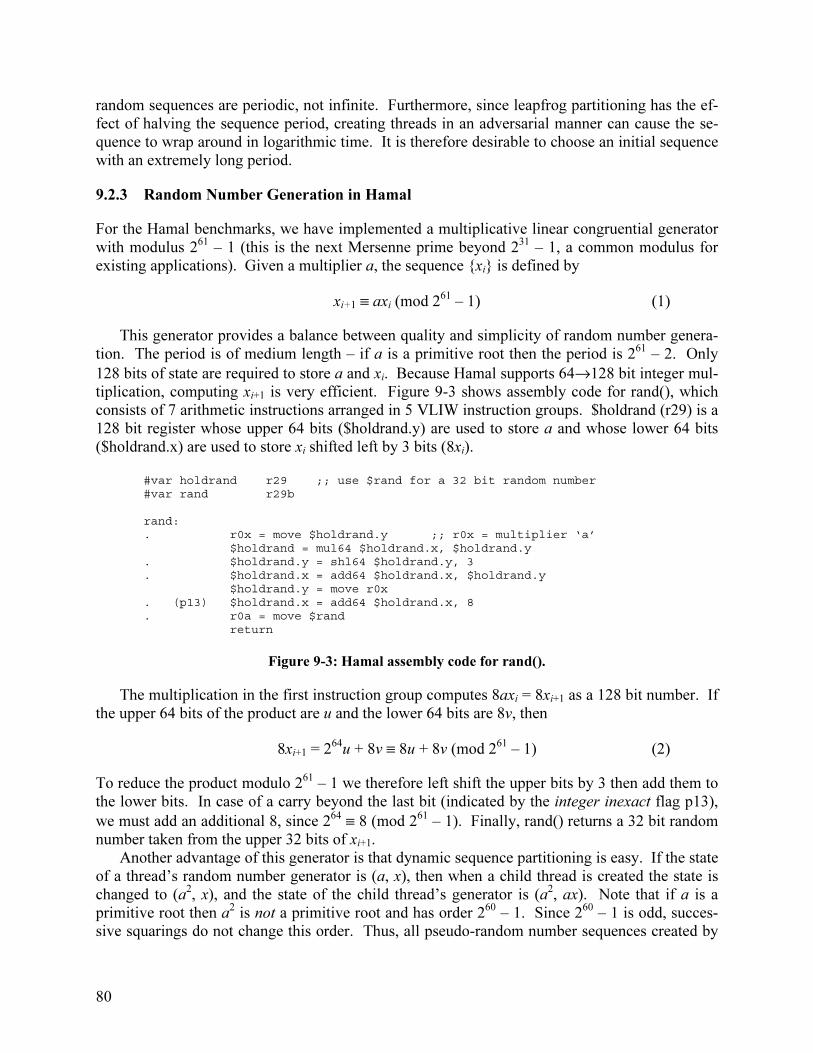
80

random sequences are periodic, not infinite. Furthermore, since leapfrog partitioning has the ef-fect of halving the sequence period, creating threads in an adversarial manner can cause the se-quence to wrap around in logarithmic time. It is therefore desirable to choose an initial sequence with an extremely long period.

9.2.3 Random Number Generation in Hamal

For the Hamal benchmarks, we have implemented a multiplicative linear congruential generator with modulus 261 – 1 (this is the next Mersenne prime beyond 231 – 1, a common modulus for existing applications). Given a multiplier a, the sequence {xi} is defined by

xi+1 ≡ axi (mod 261 – 1) (1)

This generator provides a balance between quality and simplicity of random number genera-tion. The period is of medium length – if a is a primitive root then the period is 261 – 2. Only

128 bits of state are required to store a and xi. Because Hamal supports 64→128 bit integer mul-tiplication, computing xi+1 is very efficient. Figure 9-3 shows assembly code for rand(), which consists of 7 arithmetic instructions arranged in 5 VLIW instruction groups. $holdrand (r29) is a 128 bit register whose upper 64 bits ($holdrand.y) are used to store a and whose lower 64 bits ($holdrand.x) are used to store xi shifted left by 3 bits (8xi).

#var holdrand r29 ;; use $rand for a 32 bit random number#var rand r29b

rand:. r0x = move $holdrand.y ;; r0x = multiplier ‘a’

$holdrand = mul64 $holdrand.x, $holdrand.y. $holdrand.y = shl64 $holdrand.y, 3. $holdrand.x = add64 $holdrand.x, $holdrand.y

$holdrand.y = move r0x. (p13) $holdrand.x = add64 $holdrand.x, 8. r0a = move $rand

return

Figure 9-3: Hamal assembly code for rand().

The multiplication in the first instruction group computes 8axi = 8xi+1 as a 128 bit number. If the upper 64 bits of the product are u and the lower 64 bits are 8v, then

8xi+1 = 264u + 8v ≡ 8u + 8v (mod 261 – 1) (2)

To reduce the product modulo 261 – 1 we therefore left shift the upper bits by 3 then add them to the lower bits. In case of a carry beyond the last bit (indicated by the integer inexact flag p13),

we must add an additional 8, since 264 ≡ 8 (mod 261 – 1). Finally, rand() returns a 32 bit random number taken from the upper 32 bits of xi+1.

Another advantage of this generator is that dynamic sequence partitioning is easy. If the state of a thread’s random number generator is (a, x), then when a child thread is created the state is changed to (a2, x), and the state of the child thread’s generator is (a2, ax). Note that if a is a primitive root then a2 is not a primitive root and has order 260 – 1. Since 260 – 1 is odd, succes-sive squarings do not change this order. Thus, all pseudo-random number sequences created by

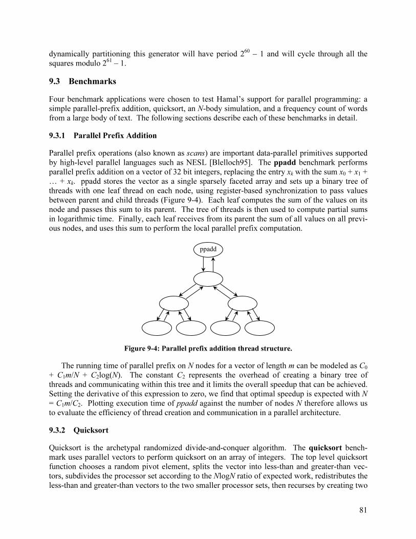
81

dynamically partitioning this generator will have period 260 – 1 and will cycle through all the squares modulo 261 – 1.

9.3 Benchmarks

Four benchmark applications were chosen to test Hamal’s support for parallel programming: a simple parallel-prefix addition, quicksort, an N-body simulation, and a frequency count of words from a large body of text. The following sections describe each of these benchmarks in detail.

9.3.1 Parallel Prefix Addition

Parallel prefix operations (also known as scans) are important data-parallel primitives supported by high-level parallel languages such as NESL [Blelloch95]. The ppadd benchmark performs parallel prefix addition on a vector of 32 bit integers, replacing the entry xk with the sum x0 + x1 + … + xk. ppadd stores the vector as a single sparsely faceted array and sets up a binary tree of threads with one leaf thread on each node, using register-based synchronization to pass values between parent and child threads (Figure 9-4). Each leaf computes the sum of the values on its node and passes this sum to its parent. The tree of threads is then used to compute partial sums in logarithmic time. Finally, each leaf receives from its parent the sum of all values on all previ-ous nodes, and uses this sum to perform the local parallel prefix computation.

Figure 9-4: Parallel prefix addition thread structure.

The running time of parallel prefix on N nodes for a vector of length m can be modeled as C0 + C1m/N + C2log(N). The constant C2 represents the overhead of creating a binary tree of threads and communicating within this tree and it limits the overall speedup that can be achieved. Setting the derivative of this expression to zero, we find that optimal speedup is expected with N = C1m/C2. Plotting execution time of ppadd against the number of nodes N therefore allows us to evaluate the efficiency of thread creation and communication in a parallel architecture.

9.3.2 Quicksort

Quicksort is the archetypal randomized divide-and-conquer algorithm. The quicksort bench-mark uses parallel vectors to perform quicksort on an array of integers. The top level quicksort function chooses a random pivot element, splits the vector into less-than and greater-than vec-tors, subdivides the processor set according to the NlogN ratio of expected work, redistributes the less-than and greater-than vectors to the two smaller processor sets, then recurses by creating two

ppadd

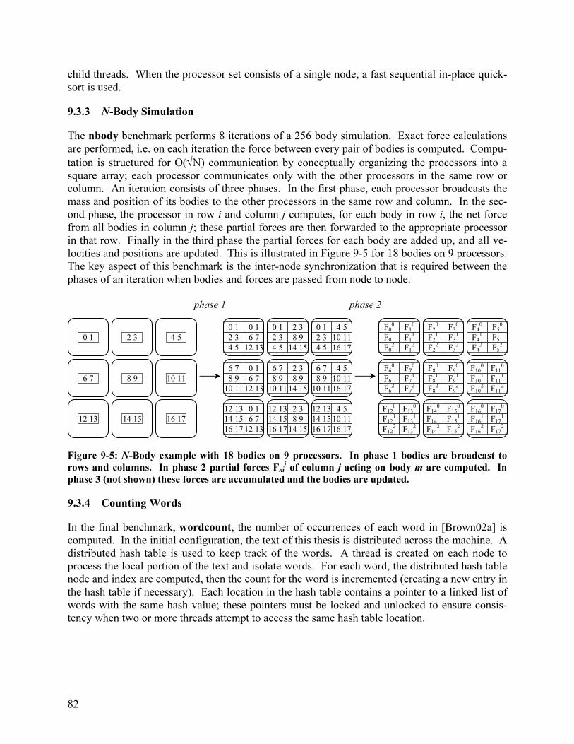
82

child threads. When the processor set consists of a single node, a fast sequential in-place quick-sort is used.

9.3.3 N-Body Simulation

The nbody benchmark performs 8 iterations of a 256 body simulation. Exact force calculations are performed, i.e. on each iteration the force between every pair of bodies is computed. Compu-

tation is structured for O(√N) communication by conceptually organizing the processors into a square array; each processor communicates only with the other processors in the same row or column. An iteration consists of three phases. In the first phase, each processor broadcasts the mass and position of its bodies to the other processors in the same row and column. In the sec-ond phase, the processor in row i and column j computes, for each body in row i, the net force from all bodies in column j; these partial forces are then forwarded to the appropriate processor in that row. Finally in the third phase the partial forces for each body are added up, and all ve-locities and positions are updated. This is illustrated in Figure 9-5 for 18 bodies on 9 processors. The key aspect of this benchmark is the inter-node synchronization that is required between the phases of an iteration when bodies and forces are passed from node to node.

Figure 9-5: N-Body example with 18 bodies on 9 processors. In phase 1 bodies are broadcast to

rows and columns. In phase 2 partial forces Fmj of column j acting on body m are computed. In

phase 3 (not shown) these forces are accumulated and the bodies are updated.

9.3.4 Counting Words

In the final benchmark, wordcount, the number of occurrences of each word in [Brown02a] is computed. In the initial configuration, the text of this thesis is distributed across the machine. A distributed hash table is used to keep track of the words. A thread is created on each node to process the local portion of the text and isolate words. For each word, the distributed hash table node and index are computed, then the count for the word is incremented (creating a new entry in the hash table if necessary). Each location in the hash table contains a pointer to a linked list of words with the same hash value; these pointers must be locked and unlocked to ensure consis-tency when two or more threads attempt to access the same hash table location.

0 1 0 1

2 3 6 7

4 5 12 13

0 1 2 3

2 3 8 9

4 5 14 15

0 1 4 5

2 3 10 11

4 5 16 17

6 7 0 1

8 9 6 7

10 11 12 13

6 7 2 3

8 9 8 9

10 11 14 15

6 7 4 5

8 9 10 11

10 11 16 17

12 13 0 1

14 15 6 7

16 17 12 13

12 13 2 3

14 15 8 9

16 17 14 15

12 13 4 5

14 15 10 11

16 17 16 17

0 1 2 3 4 5

6 7 8 9 10 11

12 13 14 15 16 17

F0

0 F1

0

F0

1 F1

1

F0

2 F1

2

F6

0 F7

0

F6

1 F7

1

F6

2 F7

2

F12

0 F13

0

F12

1 F13

1

F12

2 F13

2

F2

0 F3

0

F2

1 F3

1

F2

2 F3

2

F8

0 F9

0

F8

1 F9

1

F8

2 F9

2

F14

0 F15

0

F14

1 F15

1

F14

2 F15

2

F4

0 F5

0

F4

1 F5

1

F4

2 F5

2

F10

0 F11

0

F10

1 F11

1

F10

2 F11

2

F16

0 F17

0

F16

1 F17

1

F16

2 F17

2

phase 1 phase 2

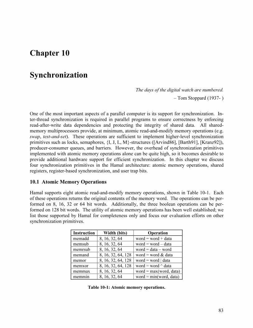
83

Chapter 10

Synchronization

The days of the digital watch are numbered.

– Tom Stoppard (1937- )

One of the most important aspects of a parallel computer is its support for synchronization. In-ter-thread synchronization is required in parallel programs to ensure correctness by enforcing read-after-write data dependencies and protecting the integrity of shared data. All shared-memory multiprocessors provide, at minimum, atomic read-and-modify memory operations (e.g. swap, test-and-set). These operations are sufficient to implement higher-level synchronization primitives such as locks, semaphores, {I, J, L, M}-structures ([Arvind86], [Barth91], [Kranz92]), producer-consumer queues, and barriers. However, the overhead of synchronization primitives implemented with atomic memory operations alone can be quite high, so it becomes desirable to provide additional hardware support for efficient synchronization. In this chapter we discuss four synchronization primitives in the Hamal architecture: atomic memory operations, shared registers, register-based synchronization, and user trap bits.

10.1 Atomic Memory Operations

Hamal supports eight atomic read-and-modify memory operations, shown in Table 10-1. Each of these operations returns the original contents of the memory word. The operations can be per-formed on 8, 16, 32 or 64 bit words. Additionally, the three boolean operations can be per-formed on 128 bit words. The utility of atomic memory operations has been well established; we list those supported by Hamal for completeness only and focus our evaluation efforts on other synchronization primitives.

Instruction Width (bits) Operation

memadd 8, 16, 32, 64 word = word + data

memsub 8, 16, 32, 64 word = word – data

memrsub 8, 16, 32, 64 word = data – word

memand 8, 16, 32, 64, 128 word = word & data

memor 8, 16, 32, 64, 128 word = word | data

memxor 8, 16, 32, 64, 128 word = word ^ data

memmax 8, 16, 32, 64 word = max(word, data)

memmin 8, 16, 32, 64 word = min(word, data)

Table 10-1: Atomic memory operations.

84

10.2 Shared Registers

The Hamal processor contains eight shared registers g0-g7 which can be read by any context and written by contexts running in privileged mode. The primary purpose of these registers is to al-low the kernel to export data to user programs, such as a pointer to the table of kernel calls and the instruction pointer for the frequently-called malloc routine. In addition, they allow shared data to be atomically read and modified by privileged-mode subroutines. Atomicity can be im-plemented by making use of both arithmetic data paths in a VLIW instruction group to simulta-neously read and write a shared register. For example, the current implementation of the Hamal microkernel uses g0 as a malloc counter; it stores the 64 bit local address at which the next seg-ment should be allocated. Figure 10-1 gives assembly code for the privileged malloc routine. The first instruction group (instruction groups are demarcated by periods) attempts to obtain the counter by simultaneously reading and resetting g0. If it is successful, the capability formed in r1 will have a non-zero address. If it is unsuccessful, indicating that another context currently holds the counter, then it spins until the counter is obtained. This implementation of malloc is extremely fast, running in only four cycles when the code is present in the instruction cache.

malloc:. r1 = gcap _CAP_BIG | _CAP_ALL, g0 ;; try to obtain the

g0 = move 0 ;; malloc counter. p0 = test r1x, r1x ;; p0 indicates success

r2 = alloc r1, r0a ;; allocate the memory. (p0) r1 = askip r1, r0a ;; advance the malloc counter

(p0) r0 = move r2 ;; return the new pointer in r0. (p0) g0 = move r1x ;; put the malloc counter back in g0

(p0) r1x = move 0 ;; destroy the big capability(p0) return

. branch malloc ;; keep trying to get the counter

Figure 10-1: Assembly code for the malloc routine, which atomically reads and modifies g0.

10.3 Register-Based Synchronization

Hamal supports register-based synchronization via the join, jcap and busy instructions. The jcap instruction creates a join capability which, when given to other threads, allows them to use the join instruction to write directly to a register in the thread that created the capability. The busy instruction marks a register as busy, which will cause a thread to stall when it attempts to access this register until another thread uses join to write to it. This is similar to register-based synchro-nization in the M-Machine [Keckler98], but differs in two important respects. First, the mecha-nism is protected via join capabilities, so mutually untrusting threads can run on the same ma-chine without worrying about unsolicited writes to their register files. Second, while the M-Machine restricts register-based synchronization to active threads running on the same physical processor, the Hamal join instruction can be used to write to an arbitrary local or remote thread in the system, and the reply event allows the microkernel to handle joins to threads which are not currently active.

One of the most important uses of register-based synchronization is to implement parent-child synchronization. A parent thread can initialize a child thread with a join capability allow-ing the child to write directly to one or more of the parent’s registers. This allows both synchro-nization and one-way communication of data. A two-way communication channel can be estab-lished if the child thread passes a join capability back to its parent.

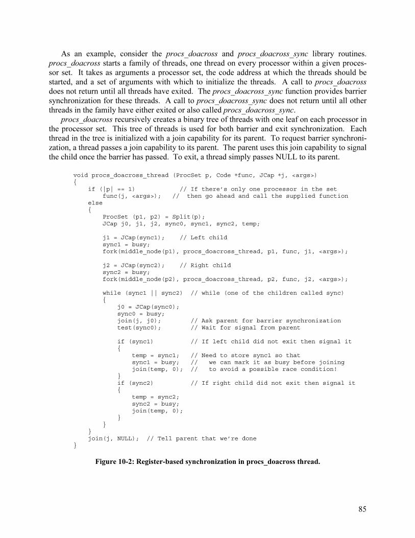
85

As an example, consider the procs_doacross and procs_doacross_sync library routines. procs_doacross starts a family of threads, one thread on every processor within a given proces-sor set. It takes as arguments a processor set, the code address at which the threads should be started, and a set of arguments with which to initialize the threads. A call to procs_doacross does not return until all threads have exited. The procs_doacross_sync function provides barrier synchronization for these threads. A call to procs_doacross_sync does not return until all other threads in the family have either exited or also called procs_doacross_sync.

procs_doacross recursively creates a binary tree of threads with one leaf on each processor in the processor set. This tree of threads is used for both barrier and exit synchronization. Each thread in the tree is initialized with a join capability for its parent. To request barrier synchroni-zation, a thread passes a join capability to its parent. The parent uses this join capability to signal the child once the barrier has passed. To exit, a thread simply passes NULL to its parent.

void procs_doacross_thread (ProcSet p, Code ∗func, JCap ∗j, <args>){

if (|p| == 1) // If there’s only one processor in the setfunc(j, <args>); // then go ahead and call the supplied function

else{

ProcSet (p1, p2) = Split(p);JCap j0, j1, j2, sync0, sync1, sync2, temp;

j1 = JCap(sync1); // Left childsync1 = busy;fork(middle_node(p1), procs_doacross_thread, p1, func, j1, <args>);

j2 = JCap(sync2); // Right childsync2 = busy;fork(middle_node(p2), procs_doacross_thread, p2, func, j2, <args>);

while (sync1 || sync2) // while (one of the children called sync){

j0 = JCap(sync0);sync0 = busy;join(j, j0); // Ask parent for barrier synchronizationtest(sync0); // Wait for signal from parent

if (sync1) // If left child did not exit then signal it{

temp = sync1; // Need to store sync1 so thatsync1 = busy; // we can mark it as busy before joiningjoin(temp, 0); // to avoid a possible race condition!

}if (sync2) // If right child did not exit then signal it{

temp = sync2;sync2 = busy;join(temp, 0);

}}

}join(j, NULL); // Tell parent that we’re done

}

Figure 10-2: Register-based synchronization in procs_doacross thread.

86

Figure 10-2 gives pseudo-code for the main procs_doacross thread. If the thread is a leaf node, it simply calls the user-supplied function and then exits. Otherwise, it splits the processor set, initiates left and right child threads, then enters a loop to service barrier requests from its children. Each barrier request is passed on to its parent. Figure 10-3 gives pseudo-code for the top-level procs_doacross function which ultimately handles all barrier requests as well as the procs_doacross_sync function which sends a barrier request to the parent thread.

void procs_doacross (ProcSet p, Code ∗func, <args>){

JCap j, sync, temp;

j = JCap(sync);sync = busy;fork(middle_node(p), procs_doacross_thread, p, func, j, <args>);

while (sync) // barrier request loop{

temp = sync;sync = busy;join(temp, 0);

}}

void procs_doacross_sync (JCap ∗j){

Word sync = busy;JCap j0 = JCap(sync);join(j, j0);test(sync);

}

Figure 10-3: Register-based synchronization in top-level procs_doacross and in barrier function.

barrier time

12

58

105

161

216

273

333

393

456

523

0

100

200

300

400

500

600

1 2 4 8 16 32 64 128 256 512

# processors

tim

e (

cycle

s)

Figure 10-4: Barrier time measured in machine cycles.

87

The time required to perform a barrier synchronization using these library functions is plotted against machine size in Figure 10-4. These times were measured as the number of machine cy-cles between consecutive barriers with no intermediate computation. We see that register-based synchronization leads to an extremely efficient software implementation of barriers which out-performs even some previously reported hardware barriers (e.g. [Kranz93]). Furthermore, be-cause no special hardware resources are required, multiple independent barrier operations may be performed simultaneously.

In a similar manner, the ppadd benchmark uses register-based synchronization to pass values between parent and child threads and to perform exit synchronization. Figure 10-5 shows a log-log plot of speedup versus machine size for ppadd on a 216 entry vector. Again, register-based synchronization permits efficient communication between threads which results in linear speedup over a wide range of machine sizes. Note that since the problem size is only 216, the amount of work performed by each thread becomes quite small beyond 64 processor nodes.

ppadd

0

1

2

3

4

5

6

7

8

1 2 4 8 16 32 64 128 256 512

# processors

log(speedup)

Figure 10-5: Speedup in parallel prefix addition benchmark.

10.4 UV Trap Bits

The fourth synchronization primitive provided in the Hamal architecture is user-controlled U and V trap bits associated with every 128-bit word of memory. Each memory operation may option-ally specify both trapping behaviour and how U and V should be modified if the operation suc-ceeds. UV traps are a generalization of previous similar mechanisms ([Smith81], [Alverson90], [Kranz92], [Keckler98]). They differ in that a trap is not returned to the thread that issued the operation. Instead, an event is generated on, and handled by, the node containing the memory word being addressed. In this section we show how UV traps can be used to implement two common forms of synchronization: producer-consumer structures and locks.

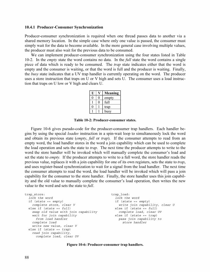
88

10.4.1 Producer-Consumer Synchronization

Producer-consumer synchronization is required when one thread passes data to another via a shared memory location. In the simple case where only one value is passed, the consumer must simply wait for the data to become available. In the more general case involving multiple values, the producer must also wait for the previous data to be consumed.

We can implement producer-consumer synchronization using the four states listed in Table 10-2. In the empty state the word contains no data. In the full state the word contains a single piece of data which is ready to be consumed. The trap state indicates either that the word is empty and the consumer is waiting, or that the word is full and the producer is waiting. Finally, the busy state indicates that a UV trap handler is currently operating on the word. The producer uses a store instruction that traps on U or V high and sets U. The consumer uses a load instruc-tion that traps on U low or V high and clears U.

U V Meaning

0 0 empty

1 0 full

0 1 trap

1 1 busy

Table 10-2: Producer-consumer states.

Figure 10-6 gives pseudo-code for the producer-consumer trap handlers. Each handler be-gins by using the special loaduv instruction in a spin-wait loop to simultaneously lock the word and obtain its previous state (empty, full or trap). If the consumer attempts to read from an empty word, the load handler stores in the word a join capability which can be used to complete the load operation and sets the state to trap. The next time the producer attempts to write to the word the store handler will be invoked which will manually complete the consumer’s load and set the state to empty. If the producer attempts to write to a full word, the store handler reads the previous value, replaces it with a join capability for one of its own registers, sets the state to trap, and uses register-based synchronization to wait for a signal from the load handler. The next time the consumer attempts to read the word, the load handler will be invoked which will pass a join capability for the consumer to the store handler. Finally, the store handler uses this join capabil-ity and the old value to manually complete the consumer’s load operation, then writes the new value to the word and sets the state to full.

trap_store:

lock the wordif (state == empty)complete store, clear V

else if (state == full)swap old value with join capabilitywait for join capability

from load handlercomplete loadwrite new value, clear V

else if (state == trap)read join capability,

complete load, clear UV

trap_load:lock the wordif (state == empty)

write join capability, clear Uelse if (state == full)

complete load, clear UVelse if (state == trap)

pass join capability tostore handler

Figure 10-6: Producer-consumer trap handlers.

89

Producer-consumer synchronization is needed between the phases of an iteration in the nbody benchmark. Two versions of this benchmark were programmed: one using UV trap bits to im-plement fine-grained producer-consumer synchronization, and one using the global barrier syn-chronization described in Section 10.3. Table 10-3 compares the run times of the two versions. For small machine sizes in which the barrier overhead is extremely low the times are roughly the same, but as the machine size and barrier overhead increase the version using fine-grained syn-chronization begins to noticeably outperform the barrier version. For 256 nodes it runs nearly 9% faster; with this many nodes 2.6% of the loads and 1.7% of the stores caused UV traps. These results are very similar to those reported in [Kranz92].

# processors 1 4 16 64 256

barrier (cycles) 38555371 9690415 2479124 665263 212725

UV (cycles) 38583457 9703698 2476991 648438 195365

speedup 0.999272 0.998631 1.000861 1.025947 1.088859

Table 10-3: Run times and speedup of UV synchronization vs. global barrier synchronization.

10.4.2 Locks

Locks are one of the most fundamental and widely used synchronization primitives. They pre-serve the integrity of shared data structures by enforcing transactional semantics. Locks have traditionally been implemented as separately-allocated data structures. In the simplest case a sin-gle bit in memory indicates whether or not a lock is available; threads acquire a lock using an atomic memory operation that reads and sets the appropriate bit, and they release a lock by clear-ing the bit. This, however, is unsatisfactory for applications that need to maintain locks for a large number of small data structures (such as individual words). There are two specific prob-lems. First, at least two extra memory references are required to access locked data: one to ac-quire the lock and one to release the lock. Second, extra storage is required for these locks. At minimum a single bit is needed for every lock, but this simple scheme only supports acquisition by spin-waiting. For more sophisticated waiting strategies involving thread blocking and wait queues, the lock must consist of at least an entire word.

In a tagged architecture with a swap instruction (such as Hamal), it is possible to finesse these problems by using a special tagged value to indicate that a word is locked. Spin-wait ac-quisition then consists of atomically swapping this LOCKED value with the desired word until it is obtained, and a lock is released simply by writing the value back to memory. This approach still requires the use of spin-waiting, the overhead of which consists of at least one test instruc-tion, one branch, and possibly a number of network messages.

U and V trap bits can be used to implement word-level locking with minimal communication and no overhead in the absence of contention. We again make use of four states, shown in Table 10-4. A word is available if it is unlocked. When a word has been locked it is unavailable and its contents are undefined. The trap state indicates that at least one thread is waiting to acquire the lock; in this state the word contains a join capability for a thread or trap handler that has re-quested the lock. As before, the busy state indicates that a trap handler is currently operating on the word. A lock is acquired using a load operation that traps on U or V high and sets U. It is released using a store operation that traps on V high and clears U.

90

U V Meaning

0 0 available

1 0 unavailable

0 1 trap

1 1 busy

Table 10-4: Locked word states.

The first time that some thread attempts to acquire an unavailable lock, the trap handler sim-ply stores a join capability for this thread in the word, sets the state to trap, and exits. Trap han-dlers invoked by subsequent acquisition attempts swap this join capability with a join capability for one of their own registers, then use register-based synchronization to wait for the lock to be released. Thus, each waiting acquire handler stores two join capabilities: one for the thread that caused the acquire trap, and one that was previously stored in the memory word. When a thread attempts to release a lock which is in the trap state, the trap handler uses the join capability stored in the memory word to pass the lock on to the next requester and sets the state to unavail-

able. Finally, when a lock is passed to a waiting acquire handler, the handler uses its first join capability to pass on the lock. It then loops back to the start to re-handle the acquisition request corresponding to its second join capability. This is illustrated in Figure 10-7.

(a) (b)

Figure 10-7: (a) Threads A, B, C, D request a lock in that order. (b) Thread A releases the lock.

In the wordcount benchmark, locks are required to preserve the integrity of the distributed hash table used to count words. In a remote access version of the benchmark, a single thread runs on each node and acquires these locks remotely. Two methods are used to acquire the locks: UV trap bits, as described above, and spin-waiting. The spin-wait version uses a special LOCKED value to acquire locks with a swap instruction, so the UV locking mechanism is being compared to the most efficient form of spin-waiting available.

Figure 10-8a gives execution time for both remote access versions of the wordcount bench-mark as the number of processors is varied from 1 to 128. As the number of processors in-creases, so too does the contention for locks. This is shows in Figure 10-8b which gives the

B

C D

B

C D

B

C D

B

B

C

B

C D

A

A

A

A

= word = lock = join capability = thread

91

number of acquire and release traps for the UV version. There is a sequential bottleneck caused by commonly occurring words such as ‘the’ (1775 occurrences) and ‘of’ (949).

With few processors (1-4) there is little contention, so the UV version marginally out-performs the spin-wait version due to the absence of test and branch instructions when a lock is acquired. For a medium number of processors (8-32) contention increases considerably, and the overhead of creating trap-handling threads in the UV version becomes a factor. Spin-waiting over a small network with few requestors is efficient enough to out-perform UV traps in this case. For a large number of processors (64+), the performance of spin-waiting becomes unac-ceptable as both the size of the network and the number of requestors increases. The perform-ance of the UV version, by contrast, remains roughly constant even as the number of trap handler threads grows past 6000. This is due to a combination of fixed communication costs, which pre-vent performance degradation, and sequential bottlenecks, which eliminate the possibility of per-formance improvements.

wordcount - remote-access version

0

500000

1000000

1500000

2000000

2500000

3000000

3500000

4000000

1 2 4 8 16 32 64 128

# processors

tim

e (

cycle

s)

spin

UV

wordcount - remote-access version

0

500

1000

1500

2000

2500

3000

3500

4000

1 2 4 8 16 32 64 128

# processors

# t

rap

sacquire traps

release traps

(a) (b)

Figure 10-8: (a) Execution time for non-forking wordcount benchmark using both spin-waiting

and UV traps. (b) Number of acquire and release traps for UV version.

These results indicate that the primary benefit of the UV trapping mechanism is the auto-matic migration of the lock-requesting task from the source node to the destination node. This has two positive effects. First, it reduces network communication for remote lock acquisition to the absolute minimum: one message to request the lock, and another message when the lock is granted. The sequence is indistinguishable from a high-latency remote memory request. Sec-ond, when a lock is heavily requested (as in the wordcount benchmark), only the node on which the lock resides spends time managing the lock. The other nodes in the system do not have to waste cycles by spin-waiting.

To verify this conjecture, local access versions of the benchmark were programmed which create a thread for each word on the node containing the word’s hash table entry. These threads then acquire locks (which are now always local) and update the hash table. With threads being manually migrated to the nodes containing the required locks, we would expect the performance advantages of the UV trapping mechanism to be lost.

Figure 10-9a plots execution times for the modified benchmark. Creating threads on the nodes containing the desired hash table entries dramatically reduces the amount of time that a given lock is held, which correspondingly lowers contention as shown in Figure 10-9b. With

92

little contention there is no noticeable difference between the spin-wait and UV versions. For 128 processors when contention becomes significant, UV trap bits are indeed outperformed by spin-waiting.

wordcount - local access

0

1

2

3

4

5

6

7

1 2 4 8 16 32 64 128

# processors

tim

e (

mil

lio

ns o

f cycle

s)

spin

UV

wordcount - local access

0

100

200

300

400

500

600

700

800

900

1 2 4 8 16 32 64 128

# processors

# t

rap

s

acquire traps

release traps

(a) (b)

Figure 10-9: (a) Execution time for forking wordcount benchmark using both spin-waiting and UV

traps. (b) Number of acquire and release traps for UV version.

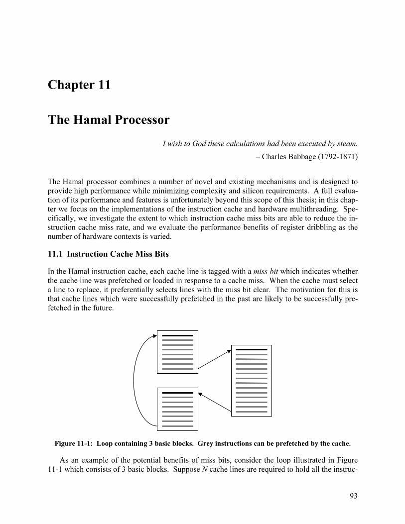
93

Chapter 11

The Hamal Processor

I wish to God these calculations had been executed by steam.

– Charles Babbage (1792-1871)

The Hamal processor combines a number of novel and existing mechanisms and is designed to provide high performance while minimizing complexity and silicon requirements. A full evalua-tion of its performance and features is unfortunately beyond this scope of this thesis; in this chap-ter we focus on the implementations of the instruction cache and hardware multithreading. Spe-cifically, we investigate the extent to which instruction cache miss bits are able to reduce the in-struction cache miss rate, and we evaluate the performance benefits of register dribbling as the number of hardware contexts is varied.

11.1 Instruction Cache Miss Bits

In the Hamal instruction cache, each cache line is tagged with a miss bit which indicates whether the cache line was prefetched or loaded in response to a cache miss. When the cache must select a line to replace, it preferentially selects lines with the miss bit clear. The motivation for this is that cache lines which were successfully prefetched in the past are likely to be successfully pre-fetched in the future.

Figure 11-1: Loop containing 3 basic blocks. Grey instructions can be prefetched by the cache.

As an example of the potential benefits of miss bits, consider the loop illustrated in Figure 11-1 which consists of 3 basic blocks. Suppose N cache lines are required to hold all the instruc-

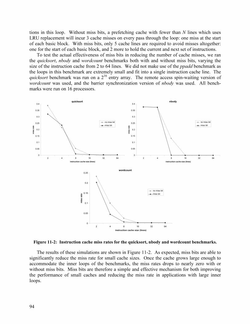
94

tions in this loop. Without miss bits, a prefetching cache with fewer than N lines which uses LRU replacement will incur 3 cache misses on every pass through the loop: one miss at the start of each basic block. With miss bits, only 5 cache lines are required to avoid misses altogether: one for the start of each basic block, and 2 more to hold the current and next set of instructions.

To test the actual effectiveness of miss bits in reducing the number of cache misses, we ran the quicksort, nbody and wordcount benchmarks both with and without miss bits, varying the size of the instruction cache from 2 to 64 lines. We did not make use of the ppadd benchmark as the loops in this benchmark are extremely small and fit into a single instruction cache line. The quicksort benchmark was run on a 216 entry array. The remote access spin-waiting version of wordcount was used, and the barrier synchronization version of nbody was used. All bench-marks were run on 16 processors.

quicksort

0

0.05

0.1

0.15

0.2

0.25

0.3

0.35

0.4

2 4 8 16 32 64

instruction cache size (lines)

mis

s r

ate

no miss bit

miss bit

nbody

0

0.05

0.1

0.15

0.2

0.25

0.3

0.35

0.4

2 4 8 16 32 64

instruction cache size (lines)

mis

s r

ate

no miss bit

miss bit

wordcount

0

0.05

0.1

0.15

0.2

0.25

2 4 8 16 32 64

instruction cache size (lines)

mis

s r

ate

no miss bit

miss bit

Figure 11-2: Instruction cache miss rates for the quicksort, nbody and wordcount benchmarks.

The results of these simulations are shown in Figure 11-2. As expected, miss bits are able to significantly reduce the miss rate for small cache sizes. Once the cache grows large enough to accommodate the inner loops of the benchmarks, the miss rates drops to nearly zero with or without miss bits. Miss bits are therefore a simple and effective mechanism for both improving the performance of small caches and reducing the miss rate in applications with large inner loops.

95

11.2 Register Dribbling

In a multithreaded architecture, register dribbling [Soundarar92] reduces the overhead of thread switching by allowing a context to be loaded or unloaded in the background while other contexts continue to perform useful computation. The Hamal processor extends this idea by maintaining a set of dirty bits for all registers and constantly dribbling the least recently issued (LRI) context to memory. Each time a dirty register is successfully dribbled (dribbling can only take place on cycles in which no thread is initiating a memory request), the register is marked as ‘clean’. We will refer to this strategy as extended dribbling.

By dribbling a context’s registers to memory in advance of the time at which the context is actually suspended, extended dribbling reduces the amount of time required to save the state of the context to memory. This in turn reduces the latency between the decision to suspend a thread and the activation of a new thread. The disadvantage of extended dribbling is that even though it makes use of cycles during which the processor is not accessing memory, a successful dribble will occupy a memory bank for the amount of time required to perform a write operation in the embedded DRAM (this is modeled as three machine cycles in the Hamal simulator). Thus, memory requests generated immediately after a dribble and targeted at the same memory bank will be delayed for two cycles.

ppadd8

0

100000

200000

300000

400000

500000

600000

700000

800000

900000

1000000

4 5 6 7 8 9 10 11 12 13 14 15 16

# contexts

tim

e (

cycle

s)

dribble on suspend

extended dribbling

quicksort

2800000

2850000

2900000

2950000

3000000

3050000

3100000

3150000

4 5 6 7 8 9 10 11 12 13 14 15 16

# contexts

tim

e (

cycle

s)

dribble on suspend

extended dribbling

nbody

2200000

2300000

2400000

2500000

2600000

2700000

2800000

2900000

4 5 6 7 8 9 10 11 12 13 14 15 16

# contexts

tim

e (

cycle

s)

dribble on suspend

extended dribbling

wordcount

0

200000

400000

600000

800000

1000000

1200000

1400000

4 5 6 7 8 9 10 11 12 13 14 15 16

# contexts

tim

e (

cycle

s)

dribble on suspend

extended dribbling

Figure 11-3: Execution time vs. number of contexts with and without extended dribbling.

96

It is impossible to determine a priori whether or not the benefits of extended dribbling out-weigh its costs, so as usual we resort to simulation. All four benchmarks were run both with and without extended dribbling with the number of hardware contexts varying from 4 to 16. With extended dribbling, a stall event is generated when there are less than two free contexts, no con-text can issue, and the LRI context is clean. Without extended dribbling this last condition is dropped, so stall events are generated sooner than they would be otherwise. Since the ppadd benchmark only creates two threads on each node (one internal node and one leaf node in the thread tree), 8 instances were run simultaneously. The quicksort benchmark was run on a 216 entry array. To maximize the number of threads, UV trap bit synchronization was used for both the nbody and wordcount benchmarks, and the local access version of wordcount was used. All benchmarks were again run on 16 processors.

The resulting execution times are shown in Figure 11-3. The two exceptional data points in the wordcount benchmark resulted from a thread being swapped out while it held a lock that was in high demand. In ppadd and wordcount, which make heavy use of thread swapping, we see that extended register dribbling offers a performance advantage (~8% in wordcount). By con-trast, both quicksort and nbody feature threads which run for long periods of time without being swapped out, so in these cases extended register dribbling actually degrades performance slightly (~1% in each case). On the whole, our initial conclusion is that extended dribbling helps more than it hurts.

We were surprised to find that increasing the number of contexts beyond 6 offers little or no performance gains in any of the benchmarks, even in ppadd8 which creates many threads on each node. Running this benchmark again with 32 simultaneous instances produces similar re-sults, shown in Figure 11-4, which graphs both execution time and processor utilization. In ret-rospect this result should not have been surprising; the simple explanation is that 6 or 7 concur-rent ppadd threads are able to fully saturate the processor’s interface to memory. This also ex-plains why extended dribbling has almost no effect with 8 or more contexts: if the processor is generating a memory request on every cycle, then the LRI context will never dribble. In the other three benchmarks, the flat performance curves are due to a lack of sufficient parallelistm.

ppadd32

0

100000

200000

300000

400000

500000

600000

700000

800000

900000

1000000

4 5 6 7 8 9 10 11 12 13 14 15 16

# contexts

tim

e (

cycle

s)

dribble on suspend

extended dribbling

ppadd32

0

0.1

0.2

0.3

0.4

0.5

0.6

0.7

0.8

0.9

1

4 5 6 7 8 9 10 11 12 13 14 15 16

# contexts

pro

cesso

r u

tili

zati

on

dribble on suspend

extended dribbling

Figure 11-4: Execution time and processor utilization vs. number of contexts for ppadd32.

97

Chapter 12

Squids

"Its head," rejoined Conseil, "was it not crowned with eight

tentacles, that beat the water like a nest of serpents?"

– Jules Verne (1828-1905), “20,000 Leagues Under the Sea”

Squids (Short Quasi-Unique IDentifiers) were introduced in Chapter 3 as a way of mitigating the effects of forwarding pointer aliasing. The theoretical motivation for squids is that by assigning a short random tag to objects, pointers to different objects can be disambiguated with high prob-ability. This avoids expensive dereferencing operations when performing pointer comparisons, and prevents the processor from having to wait for every split-phase memory operation to com-plete before initiating the next one. In this chapter we discuss experiments performed using the Hamal simulator to quantify the performance advantages of squids.

12.1 Benchmarks

Table 12-1 lists the eight benchmarks used to evaluate squids. The first five (list, 2cycle, kruskal, fibsort, sparsemat) involve pointer comparisons and the primary overhead is traps taken to determine final addresses. The last three (vector, filter, listrev) involve rapid loads/stores and the primary overhead is memory stalls when addresses cannot be disambiguated.

It was necessary to carefully choose these benchmarks as most programs either do not make use of pointer comparisons, or compare them so infrequently that slow comparisons would have no impact on performance. Nonetheless, as exemplified by the benchmarks, there are some fun-damental data structures for which pointer comparisons are frequently used. One common ex-ample is graphs, in which pointer comparisons can be used to determine whether two vertices are the same. Both 2cycle and kruskal are graph algorithms. 2cycle uses a brute force approach to detect 2-cycles in a directed graph by having each vertex look for itself in the connection lists of its neighbours. kruskal uses Kruskal’s minimum spanning tree algorithm [CLR90] in which edges are chosen greedily without creating cycles. To avoid cycles, a representative vertex is maintained for every connected sub-tree during construction, and an edge may be selected only if the vertices it connects have different representatives.

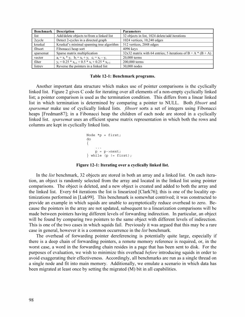
98

Benchmark Description Parameters

list Add/delete objects to/from a linked list 32 objects in list, 1024 delete/add iterations

2cycle Detect 2-cycles in a directed graph 1024 vertices, 10,240 edges

kruskal Kruskal’s minimal spanning tree algorithm 512 vertices, 2048 edges

fibsort Fibonacci heap sort 4096 keys

sparsemat Sparse matrix multiplication 32x32 matrix with 64 entries; 5 iterations of B = A * (B + A)

vector ai = xi * yi bi = xi + yi ci = xi – yi 20,000 terms

filter yi = 0.25 * xi-1 + 0.5 * xi + 0.25 * xi+1 200,000 terms

listrev Reverse the pointers in a linked list 30,000 nodes

Table 12-1: Benchmark programs.

Another important data structure which makes use of pointer comparisons is the cyclically linked list. Figure 2 gives C code for iterating over all elements of a non-empty cyclically linked list; a pointer comparison is used as the termination condition. This differs from a linear linked list in which termination is determined by comparing a pointer to NULL. Both fibsort and sparsemat make use of cyclically linked lists. fibsort sorts a set of integers using Fibonacci heaps [Fredman87]; in a Fibonacci heap the children of each node are stored in a cyclically linked list. sparsemat uses an efficient sparse matrix representation in which both the rows and columns are kept in cyclically linked lists.

Node *p = first;do{

...p = p->next;

} while (p != first);

Figure 12-1: Iterating over a cyclically linked list.

In the list benchmark, 32 objects are stored in both an array and a linked list. On each itera-tion, an object is randomly selected from the array and located in the linked list using pointer comparisons. The object is deleted, and a new object is created and added to both the array and the linked list. Every 64 iterations the list is linearized [Clark76]; this is one of the locality op-timizations performed in [Luk99]. This benchmark is somewhat contrived; it was constructed to provide an example in which squids are unable to asymptotically reduce overhead to zero. Be-cause the pointers in the array are not updated, subsequent to a linearization comparisons will be made between pointers having different levels of forwarding indirection. In particular, an object will be found by comparing two pointers to the same object with different levels of indirection. This is one of the two cases in which squids fail. Previously it was argued that this may be a rare case in general, however it is a common occurrence in the list benchmark.

The overhead of forwarding pointer dereferencing is potentially quite large, especially if there is a deep chain of forwarding pointers, a remote memory reference is required, or, in the worst case, a word in the forwarding chain resides in a page that has been sent to disk. For the purposes of evaluation, we wish to minimize this overhead before introducing squids in order to avoid exaggerating their effectiveness. Accordingly, all benchmarks are run as a single thread on a single node and fit into main memory. Additionally, we emulate a scenario in which data has been migrated at least once by setting the migrated (M) bit in all capabilities.

99

12.2 Simulation Results

Figure 12-2 shows the results of running all eight benchmark programs with the number of squid bits varying from 0 to 8. Execution time is broken down into program cycles, trap handler cy-cles, and memory stalls. A cycle is counted as a memory stall when the hardware is unable to disambiguate different addresses and as a result a memory operation is blocked. Table 12-2 lists the total speedup of the benchmarks over their execution time with zero squid bits.

As expected, in most cases the overhead due to traps and memory stalls drops exponentially to zero as the number of squid bits increases. The three exceptions are list, vector and filter. In vector and filter the lack of a smooth exponential curve is simply due to the small number of dis-tinct objects (five in vector, two in filter), so in both cases the overhead steps down to zero once all objects have distinct squids. In list the overhead drops exponentially to a non-zero amount. This is because squids offer no assistance in comparisons of two pointers to the same object with different levels of indirection.

Squid bits: 1 2 3 4 5 6 7 8

list 1.57 2.22 2.76 3.16 3.41 3.55 3.62 3.65

2cycle 1.66 2.47 3.27 3.91 4.32 4.56 4.68 4.75

kruskal 1.01 1.02 1.02 1.02 1.02 1.03 1.03 1.03

fibsort 1.26 1.46 1.58 1.65 1.69 1.70 1.71 1.72

sparsemat 1.62 2.24 2.83 3.41 3.57 3.92 3.98 4.00

vector 1.18 1.30 1.30 1.30 1.30 1.30 1.30 1.30

filter 1.00 1.12 1.12 1.12 1.12 1.12 1.12 1.12

listrev 1.09 1.14 1.17 1.18 1.19 1.20 1.20 1.20

Table 12-2: Speedup over execution time with zero squid bits.

We note that squids are most effective in programs that compare pointers within the inner loop. This includes list, 2cycle, fibsort and sparsemat, where the speedup with eight squid bits ranges from 1.72 for fibsort to 4.75 for 2cycle. In kruskal, by contrast, the inner loop follows a chain of pointers to find a vertex’s representative; only once the representatives for two vertices have been found is a pointer comparison performed. As a result, the improvement in perform-ance due to squids is barely noticeable.

Squids are also helpful, albeit to a lesser extent, in the three memory-intensive benchmarks. With eight squid bits the speedup ranges from 1.12 in filter to 1.30 in vector. Note that in each of these benchmarks, as the number of squid bits is raised the decrease in overall execution time is slightly less than the decrease in the number of memory stalls. This is because programs are allowed to continue issuing arithmetic instructions while a memory request is stalled, so in some cases there is overlap between memory stalls and program execution. Overlap cycles have been graphed as memory stall cycles.

100

list

0

0.2

0.4

0.6

0.8

1

1.2

1.4

0 1 2 3 4 5 6 7 8

2cycle

0

1

2

3

4

5

6

7

0 1 2 3 4 5 6 7 8

kruskal

0

0.1

0.2

0.3

0.4

0.5

0.6

0.7

0.8

0.9

0 1 2 3 4 5 6 7 8

fibsort

0

1

2

3

4

5

6

7

8

0 1 2 3 4 5 6 7 8

sparsemat

0

0.5

1

1.5

2

2.5

3

3.5

4

0 1 2 3 4 5 6 7 8

vector

0

0.05

0.1

0.15

0.2

0.25

0.3

0.35

0.4

0.45

0 1 2 3 4 5 6 7 8

filter

0

0.5

1

1.5

2

2.5

3

0 1 2 3 4 5 6 7 8

listrev

0

0.05

0.1

0.15

0.2

0.25

0.3

0 1 2 3 4 5 6 7 8

Figure 12-2: Squid simulation results. For each benchmark the horizontal axis indicates the num-

ber of squid bits used and the vertical axis gives the execution time in millions of cycles. Execution

time is broken down into program cycles, trap handler cycles and memory stall cycles.

program execution trap handler memory stall

101

12.3 Extension to Other Architectures

The design space of capability architectures is quite large, so we must call into question the ex-

tent to which our results would generalize to other architectures. In particular, the execution

time of the trap handler (which is roughly 48 cycles from start to finish in our simulations) may

be significantly smaller in an architecture with data caches or extra registers available to the trap

handler. However, we note that:

1. Any mechanism that speeds up the trap handler but is not specific to traps (e.g. data

caches, out-of-order execution) will most likely reduce program execution time compara-

bly, keeping the percentage of trap handler cycles the same.

2. Hardware improvements reduce the cost but not the number of traps. Squids reduce the

number of traps exponentially independent of the architecture.

The number of memory operations that the hardware fails to reorder or issue simultaneously

is architecture dependent since it is affected by such factors as memory latency and the size of

the instruction reorder buffer (if there is one). If the overhead due to memory stalls in memory

intensive applications is negligible to begin with, then the architecture will not benefit from add-

ing squids to the memory controller logic. On the other hand if the overhead is noticeable, then

squids will reduce it exponentially.

12.4 Alternate Approaches

We have focused our evaluations on the specific implementation of squids in the Hamal architec-

ture, i.e. a hardware-recognized field within capabilities. A number of other approaches to the

problem of pointer disambiguation can be used in place of or in addition to this technique.

12.4.1 Generation Counters

We can associate with each pointer an m bit saturating generation counter which indicates the

number of times that the object has been migrated. If two pointers being compared have the

same generation counter (and it has not saturated), then the hardware can simply compare the

address fields directly.

The migrated (M) bit in Hamal capabilities is a single-bit generation counter that deals with

the common case of objects that are never migrated. This completely eliminates aliasing over-

head for applications that choose not to make use of forwarding pointers. Using two generation

bits handles the additional case in which objects are migrated exactly once as a compaction op-

eration after the program has initialized its data (this is one of the techniques used in [Luk99]).

Again, overhead is completely eliminated in this case.

More generally, generation counters are effective in programs for which (1) objects are mi-

grated a small number of times, and (2) at all times most working pointers to a given object have

the same level of indirection. They lose their effectiveness in programs for which either of these

statements is false.

102

12.4.2 Software Comparisons

Instead of relying on hardware to ensure the correctness of pointer comparisons, the compiler

can insert code to explicitly determine the final addresses and then compare them directly, as in

[Luk99]. Figure 12-3 shows the code that must be inserted; for each pointer a copy is created,

and the copy is replaced with the final address by repeatedly checking for the presence of a

forwarding pointer in the memory word being addressed. The outer loop is required in systems

that support concurrent garbage collection or object migration to avoid a race condition when an

object is migrated while the final addresses are being computed. In a complex superscalar

processor, the cost of this code may only be a few cycles (and a few registers) if the memory

words being addressed are present in the data cache. The overhead will be much larger if a

cache miss occurs while either of the final addresses is being computed.

temp1 = ptr1;temp2 = ptr2;flag = 0;do{

while (check_forwarding_bit(temp1))temp1 = unforwarded_read(temp1);

while (check_forwarding_bit(temp2)){

temp2 = unforwarded_read(temp2);flag = 1;

}} while (flag);compare(temp1, temp2);

Figure 12-3: Using software only to ensure the correctness of pointer comparisons, the compiler

must insert the above code wherever two pointers are compared.

Making use of hardware traps, and placing this code in a trap handler rather than inlining it at

every pointer comparison, has the advantages of reducing code size and eliminating overhead

when the hardware is able to disambiguate the pointers. On the other hand, overhead is in-

creased when a trap is taken due to the need to initialize the trap handler and clean up when it has

finished. In our simulations, we found that 25% of the trap cycles were used to perform the ac-

tual comparisons. Thus, using software comparisons would give roughly the same performance

as hardware comparisons with two squid bits.

The cost of software comparisons can be reduced (but not eliminated) by incorporating

squids, as shown in Figure 5. This combined approach features both exponential reduction in

overhead and fast inline comparisons at the expense of increased code size and register require-

ments.

temp = ptr1 ^ ptr2;if (temp & SQUID_MASK)

<pointers are different>else

<compare by dereferencing>

Figure 12-4: Using squids in conjunction with software comparison.

103

12.4.3 Data Dependence Speculation

In [Luk99], the problem of memory operation reordering is addressed using data dependence

speculation ([Moshovos97], [Chrysos98]). This is a technique that allows loads to speculatively

execute before an earlier store when the address of the store is not yet known. In order to sup-

port forwarding pointers, the speculation mechanism must be altered so that it compares final

addresses rather than the addresses initially generated by the instruction stream. This in turn re-

quires that the mechanism is somehow informed each time a memory request is forwarded. The

details of how this is accomplished would depend on whether forwarding is implemented di-

rectly by hardware or in software via exceptions.

Data dependence speculation does not allow stores to execute before earlier loads/stores, but

this is unlikely to cause problems as a store does not produce data which is needed for program

execution. A greater concern is the failure to reorder atomic read-and-modify memory opera-

tions, such as those supported by the Tera [Alverson90], the Cray T3E [Scott96], or Hamal.

12.4.4 Squids without Capabilities

It is possible to implement squids without capabilities by taking the upper n bits of a pointer to

be that pointer’s squid. This has the effect of subdividing the virtual address space into 2n

do-

mains. When an object is allocated, it is randomly assigned to one of the domains. Objects mi-

gration is then restricted to a single domain in order to preserve squids.

Using a large number of domains introduces fragmentation problems and makes data com-

paction difficult since, for example, objects from different domains cannot be placed in the same

page. However, as seen in Section 12.2, noticeable performance improvements are achieved

with only one or two squid bits (two or four domains).

Alternately, the hardware can cooperate to avoid the problems associated with multiple do-

mains by simply ignoring the upper n address bits. In this case the architecture begins to resem-

ble a capability machine since the pointer contains both an address and some additional informa-

tion. The difference is that the pointers are unprotected, so user programs must take care to

avoid mutating the squid bits or performing pointer arithmetic that causes a pointer to address a

different object. Additionally, because the pointer contains no segment information, arrays of

objects are still a problem since a single squid would be created for the entire array.

12.5 Discussion

Forwarding pointers facilitate safe data compaction, object migration, and efficient garbage col-

lection. In order to address the aliasing problems that arise, the Hamal architecture implements

squids, which allow the hardware to, with high probability, disambiguate pointers in the presence

of aliasing without performing expensive dereferencing operations. Our experimental results

show that squids provide significant performance improvements on the small but important set of

applications that suffer from aliasing, speeding up some programs by over a factor of four.

The fact that the overhead associated with forwarding pointer support diminishes exponen-

tially with the number of squid bits has two important consequences. First, very few squid bits

are required to produce considerable performance improvements. Even a single squid bit pro-

vides noticeable speedups on the majority of the benchmarks, and as Figure 12-2 shows, most of

the potential performance gains can be realized with four bits. Thus, squids remain appealing in

architectures which have few capability bits to spare. Second, squids allow an architecture to

104

tolerate slow traps and/or long memory latencies while determining final addresses. For most

applications, three or four additional squid bits would compensate for an order of magnitude in-

crease in the time required to execute the pointer comparison code of Figure 12-3.

105

Chapter 13

Analytically Modeling a Fault-Tolerant Messaging

Protocol

Models are to be used, not believed.

– Henri Theil (1924-2000), “Principles of Econometrics”

Analytical models are an important tool for the study of network topologies, routing protocols

and messaging protocols. They allow evaluations to be conducted without expensive simulations

that can take hours or even days to complete. However, analytically modeling a fault-tolerant

messaging protocol is challenging for several reasons:

• There are multiple packet types (at least two are required: ‘message’ and ‘acknowledge’)

• Many packets must be re-sent

• The future behaviour of the network depends on which packets have been successfully

received

In this chapter we present a simple approach to the analysis of fault-tolerant protocols that

accurately models these effects while hiding many of the other protocol details. We are able to

solve for key performance parameters by considering only the rates at which the different types

of packets are sent and the probabilities that they are dropped at various points in the network

once the system has reached a steady state. Our method is quite general and can be applied to

various topologies and routing strategies. We will demonstrate the accuracy of the models ob-

tained by comparing them to simulated results for the idempotent messaging protocol described

in Chapter 5 implemented using both circuit switching and wormhole routing on three different

network topologies.

The literature contains a myriad of analytical models for dynamic network behaviour. Mod-

els have been proposed for specific network topologies ([Dally90], [Stamoulis91], [Saleh96],

[Greenberg97]), routing algorithms ([Draper94], [Sceideler96], [Ould98]), and traffic patterns

[Sarbazi00]. While the vast majority of this work has focused on non-discarding networks, dis-

carding networks have also been considered ([Parviz79], [Rehrmann96], [Datta97]). However,

in [Rehrmann96] and [Datta97] packet retransmission was not modeled. In [Parviz79] the model

did take into account packet retransmission, but a magic protocol was used whereby the sending

node was instantly and accurately informed as to the success or failure of a packet. Our work

differs from previous research in that we present an accurate model for the higher-level messag-

ing protocol required to ensure packet delivery across a faulty network.

106

13.1 Motivating Problem

Our work was motivated by an attempt to analytically answer the following question: Given a

desire to implement the idempotent messaging protocol on a bisection-limited network, should

one use wormhole routing or circuit switching? In a wormhole routed network, all three protocol

packets are independently routed through the network; all three are subject to being discarded

due to contention within the network. In a circuit switched network, only the MSG packet is

routed through the network. A connection is maintained along the path that it takes, and the

ACK and CONF packets are sent through this connection. They can still be lost due to corrup-

tion, but not due to contention. On one hand, wormhole routing generally makes more efficient

use of network resources. On the other hand, circuit switching capitalizes on a successful MSG

route through the network bisection by holding the channel open for the ACK and CONF pack-

ets. We will answer this question in Section 13.3.4 after deriving models for both wormhole

routing and circuit switching on a bisection-limited network.

13.2 Crossbar Network

To introduce our technique, we begin with the simplest of networks: a crossbar. Specifically, we

assume a pipelined crossbar of diameter d where the head of each packet takes d cycles to reach

its destination and there is no contention within the network. Each node has one receive port.

When a packet reaches its destination node it is delivered if the receive port is free and it is dis-

carded otherwise.

In all that follows, we assume that each node generates messages independently at an average

rate of λ messages per cycle, and that message destinations are chosen randomly. MSG packets

are L flits long; ACK and CONF packets are each m flits long. For all networks that we con-

sider, we assume that packets are lost due to contention only. We do not model network failures.

13.2.1 Circuit Switched Crossbar

To derive our models, we use the standard approach of assuming that the network reaches a

steady state and then solving for the steady state parameters. For uniform traffic on a circuit

switched crossbar, there are two parameters of interest: the rate α at which each node attempts to

send messages, and the probability p that a message is successfully delivered when it reaches its

destination.

With only two parameters, we need only two equations. Our first equation comes from con-

servation of messages: messages must be successfully delivered at the same rate that they are

generated, hence

λ = αp (1)

Our second equation comes from port utilization: the probability that a message is dropped at

the receive node (1 – p) is equal to the probability that the receive port is in use. When a mes-

sage is dropped, it uses zero receive port cycles. Using circuit switching, when a message is suc-

cessfully received it uses 2d + L + 2m receive port cycles (L cycles to absorb the MSG packet, d

cycles to send the ACK packet to the sender, m cycles for that packet to be absorbed, d cycles to

send the CONF packet to the receiver, finally m cycles for that packet to be absorbed). Thus,

each node causes receive port cycles to be used at a rate of αp(2d + L + 2m). Since the number

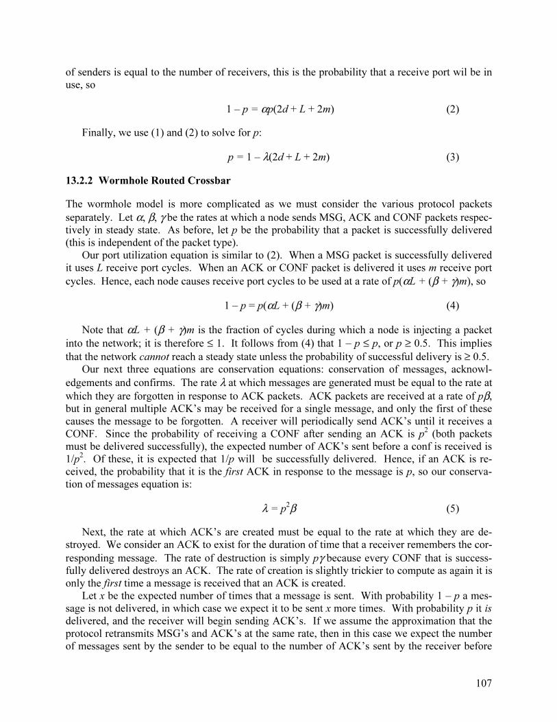
107

of senders is equal to the number of receivers, this is the probability that a receive port wil be in

use, so

1 – p = αp(2d + L + 2m) (2)

Finally, we use (1) and (2) to solve for p:

p = 1 – λ(2d + L + 2m) (3)

13.2.2 Wormhole Routed Crossbar

The wormhole model is more complicated as we must consider the various protocol packets

separately. Let α, β, γ be the rates at which a node sends MSG, ACK and CONF packets respec-

tively in steady state. As before, let p be the probability that a packet is successfully delivered

(this is independent of the packet type).

Our port utilization equation is similar to (2). When a MSG packet is successfully delivered

it uses L receive port cycles. When an ACK or CONF packet is delivered it uses m receive port

cycles. Hence, each node causes receive port cycles to be used at a rate of p(αL + (β + γ)m), so

1 – p = p(αL + (β + γ)m) (4)

Note that αL + (β + γ)m is the fraction of cycles during which a node is injecting a packet

into the network; it is therefore ≤ 1. It follows from (4) that 1 – p ≤ p, or p ≥ 0.5. This implies

that the network cannot reach a steady state unless the probability of successful delivery is ≥ 0.5.

Our next three equations are conservation equations: conservation of messages, acknowl-

edgements and confirms. The rate λ at which messages are generated must be equal to the rate at

which they are forgotten in response to ACK packets. ACK packets are received at a rate of pβ,

but in general multiple ACK’s may be received for a single message, and only the first of these

causes the message to be forgotten. A receiver will periodically send ACK’s until it receives a

CONF. Since the probability of receiving a CONF after sending an ACK is p2 (both packets

must be delivered successfully), the expected number of ACK’s sent before a conf is received is

1/p2. Of these, it is expected that 1/p will be successfully delivered. Hence, if an ACK is re-

ceived, the probability that it is the first ACK in response to the message is p, so our conserva-

tion of messages equation is:

λ = p2β (5)

Next, the rate at which ACK’s are created must be equal to the rate at which they are de-

stroyed. We consider an ACK to exist for the duration of time that a receiver remembers the cor-

responding message. The rate of destruction is simply pγ because every CONF that is success-

fully delivered destroys an ACK. The rate of creation is slightly trickier to compute as again it is

only the first time a message is received that an ACK is created.

Let x be the expected number of times that a message is sent. With probability 1 – p a mes-

sage is not delivered, in which case we expect it to be sent x more times. With probability p it is

delivered, and the receiver will begin sending ACK’s. If we assume the approximation that the

protocol retransmits MSG’s and ACK’s at the same rate, then in this case we expect the number

of messages sent by the sender to be equal to the number of ACK’s sent by the receiver before

108

one is received. This in turn is 1/p since the probability of a given ACK being received is p. It

follows that:

x = p(1/p) + (1 – p)(x + 1) (6)

Solving for x:

x = 2/p – 1 (7)

The expected number of times a message is received is therefore px = 2 – p. Thus, when a

message is received the probability that it is the first copy received (and hence creates an ACK)

is 1/(2 – p), so our equation for conservation of ACK’s is:

pα / (2 – p) = pγ (8)

which we rewrite as:

α = (2 – p)γ (8’)

Finally, a CONF is created every time an ACK is received and it is forgotten as soon as it is

sent, so our equation for conservation of CONF’s is:

γ = pβ (9)

Let T = 1/λ, so T is the average amount of time in cycles between the generation of new mes-

sages on a node. Eliminating α, β, γ from equations (4), (5), (8) and (9) leaves us with the fol-

lowing quadratic in p:

f(p) = (T – L)p2 + (2L + m – T)p + m = 0 (10)

Solving for p:

)(2

)(

LT

mLLTp

−∆±−−−= (11)

Where ∆ is the discriminant of f. Recall that for the solution to be meaningful we must have p

≥ 0.5. But if f has real roots then we see from (11) that the smaller root is less than 0.5, so it is

the larger root that we are interested in. Furthermore, f(1) = L + 2m > 0, so it follows that f has a

real root in [0.5, 1) if and only if f(0.5) ≤ 0. Substituting this into (9) gives us the following nec-

essary and sufficient condition for a meaningful solution to exist:

T ≥ 3(L + 2m) (12)

13.2.3 Comparison with Simulation

Simulations were performed of the idempotent messaging protocol using both circuit switching

and wormhole routing on a crossbar network with d = 10. On every simulated cycle a node gen-

erates a new message to send with probability λ. A node’s send queue is allowed to grow arbi-

109

trarily long, and nodes are always able to accept packets from the network so long as their re-

ceive port is free. For the wormhole network, MSG and ACK packets are retransmitted at a

fixed interval of twice the network round-trip latency Additionally, if a node has more than one

packet which is ready to be sent, preference is given to ACK and CONF packets.

In Figure 13-1 we compare the results of the simulations to the predictions of our models for

three different values of L and m. The graphs plot p, the probability of successful delivery, ver-

sus T, the average time between message generation on a node. In all cases the model agrees

closely with simulation results. Note that the graphs diverge slightly for small values of T on a

circuit switched network. This is due to the fact that in simulation a steady state was never

reached for these values of T; the size of the send queues continued to increase for the duration

of the simulation.

L = 10, l = 1, d = 10

0.3

0.4

0.5

0.6

0.7

0.8

0.9

1

50 90 130 170 210 250

T

p

L = 5, l = 1, d = 10

0.3

0.4

0.5

0.6

0.7

0.8

0.9

1

50 90 130 170 210 250

T

p

L = 7, l = 2, d = 10

0.3

0.4

0.5

0.6

0.7

0.8

0.9

1

50 90 130 170 210 250

T

p

Figure 13-1: Simulated and predicted values of p plotted against T for both circuit switched and

wormhole routed crossbar networks.

The probability p is all that is required to determine the performance characteristics of the

network. For example, in the wormhole routed network the expected number of message trans-

missions is given by (7), and in both networks the expected latency from initial message trans-

mission to message reception is

Rp

pLd

−++ 1 (13)

where R is the retransmission interval for a message packet. Note that the value of p does not

depend on R; this is one of the ways in which our model hides the details of the protocol imple-

mentation. Our only assumption has been that the same retransmission interval is used for both

MSG and ACK packets.

13.2.4 Improving the Model

Inspecting the graphs of Figure 13-1 reveals a small but consistent discrepancy between the

model and simulation. This is most noticeable for wormhole routing with L = 5, 7. The source

of this error is an inaccuracy in our port utilization equations (2) and (4). In deriving these equa-

tions, we made the assumption that in steady state a fixed fraction of receive ports are always in

use, and that this fraction is the probability of a message being dropped. However, in a discrete

time system this is not quite correct, because at the start of each cycle some fraction of receive

ports will become available, then later in the same cycle the same expected number of ports will

become occupied with new packets.

wormhole routed model

wormhole routed simulation

circuit switched model

circuit switched simulation

110

In the wormhole network, the expected fraction of busy receive ports that become available

at the start of a cycle is 1/(expected packet length), i.e.

mL )( γβα

γβα++++

(14)

so the actual fraction x of receive ports that are in use at the start of a cycle is:

))1)(()1((

)(1))((

−++−=

++++

−++=

mLp

mLmLpx

γβαγβαγβαγβα

(15)

If we randomly order the new packets competing for receive ports and attempt to deliver

them in that order, then x is the probability that the first of these packets will encounter a busy

port. As more packets are delivered this probability increases, until finally the probability that

the last packet encounters a busy port is very nearly

p(αL + (β + γ)m) (16)

A reasonable approximation is therefore to assume that all new packets encounter a busy re-

ceive port with probability midway between above two probabilities. This gives the following

revised port utilization equation:

1 – p = p(α(L – ½) + (β + γ)(m – ½)) (17)

Using equations (5), (8) and (9) once again to eliminate α, β, γ gives us the same quadratic

(10) and solution (11) as before but with L, m replaced by L – ½, m – ½. Figure 13-2 shows p

plotted against T with d = 10, L = 5 and m = 1 for the original model, the simulation, and the re-

vised model. We see that the revised model gives a much closer match to the simulation results.

For the remainder of the chapter we will use this improved model when considering wormhole

routed networks; for circuit switched networks we will continue to use the original model as the

inaccuracy is less pronounced.

L = 5, m = 1, d = 10

0.5

0.6

0.7

0.8

0.9

1

20 70 120 170 220

T

p

model

revised model

simulation

Figure 13-2: p plotted against T in a wormhole routed network. Shown are the original model, the

simulation results, and the revised model based on the corrected port utilization equation.

111

13.3 Bisection-Limited Network

We now shift our attention to the subject of our motivating problem: a network whose perform-

ance is limited by its bisection bandwidth. Figure 13-3 illustrates the network model that we use.

There are N nodes in each half of the network, and the bisection consists of k ports in either di-

rection. We model each half of the network as a crossbar, so that the nodes and bisection ports

are fully connected. Both crossbars are again pipelined with diameter d. We will refer to a

packet’s destination as remote if it is on the other side of the bisection and local otherwise. A

remotely destined packet is randomly routed to one of the bisection ports; if the port is free the

packet passes through, otherwise it is dropped.

Figure 13-3: Bisection-limited network model.

13.3.1 Circuit Switched Network

Our circuit switched model now consists of four steady state parameters. Let α0, α1 be the rates

at which a node attempts to send messages with local and remote destinations respectively. Let

p0 be the probability of successful delivery once a packet reaches its destination; let p1 be the

probability that a packet with a remote destination is able to cross the bisection. L, m, λ and T

are as defined previously.

We now have two conservation of messages equations: one for local messages and one for

remote messages. Since destinations are randomly chosen and, from a given node, exactly half

of the destinations are remote, it follows that a node generates both local and remote messages at

a rate of λ/2. The probability of successful delivery for a local message is p0, and for a remote

message it is p0p1. Our conservation equations are therefore:

λ/2 = p0α0 (18)

λ/2 = p0p1α1 (19)

We also have two port utilization equations: one for receive ports and one for bisection ports.

If a node successfully sends a local message it uses 2d + L + 2m receive port cycles as in Section

13.2.1. Similarly, a successful remote message uses 4d + L + 2m receive port cycles. Again, the

probability that a receive port is in use is equal to the rate at which receive port cycles are used,

so

1 – p0 = p0α0 (2d + L + 2m) + p0p1α1 (4d + L + 2m)

= λ(3d + L + 2m) (using (18), (19))

⇒ p0 = 1 – λ(3d + L + 2m) (20)

N N

k

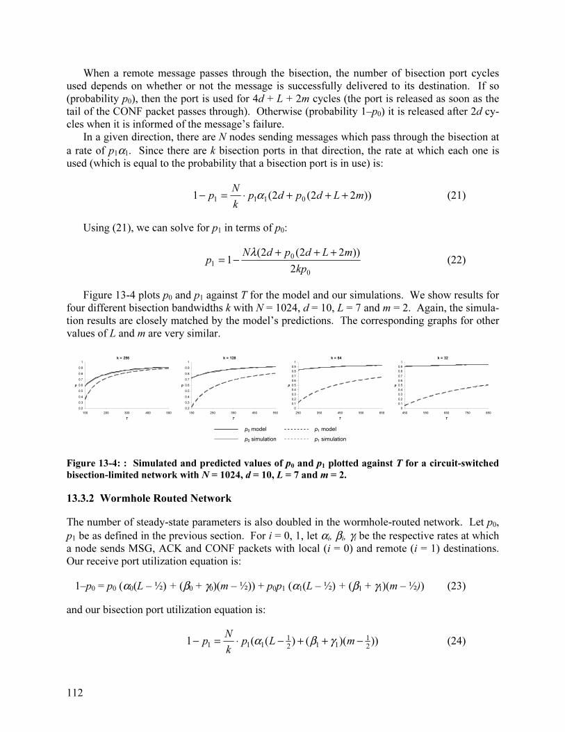
112

When a remote message passes through the bisection, the number of bisection port cycles

used depends on whether or not the message is successfully delivered to its destination. If so

(probability p0), then the port is used for 4d + L + 2m cycles (the port is released as soon as the

tail of the CONF packet passes through). Otherwise (probability 1–p0) it is released after 2d cy-

cles when it is informed of the message’s failure.

In a given direction, there are N nodes sending messages which pass through the bisection at

a rate of p1α1. Since there are k bisection ports in that direction, the rate at which each one is

used (which is equal to the probability that a bisection port is in use) is:

))22(2(10111

mLdpdpk

Np +++⋅=− α (21)

Using (21), we can solve for p1 in terms of p0:

0

0

12

))22(2(1

kp

mLdpdNp

+++−=

λ (22)

Figure 13-4 plots p0 and p1 against T for the model and our simulations. We show results for

four different bisection bandwidths k with N = 1024, d = 10, L = 7 and m = 2. Again, the simula-

tion results are closely matched by the model’s predictions. The corresponding graphs for other

values of L and m are very similar.

k = 256

0.2

0.3

0.4

0.5

0.6

0.7

0.8

0.9

1

100 200 300 400 500

T

p

k = 128

0.2

0.3

0.4

0.5

0.6

0.7

0.8

0.9

1

150 250 350 450 550

T

p

k = 64

0

0.1

0.2

0.3

0.4

0.5

0.6

0.7

0.8

0.9

1

250 350 450 550 650

T

p

k = 32

0

0.1

0.2

0.3

0.4

0.5

0.6

0.7

0.8

0.9

1

450 550 650 750 850

T

p

Figure 13-4: : Simulated and predicted values of p0 and p1 plotted against T for a circuit-switched

bisection-limited network with N = 1024, d = 10, L = 7 and m = 2.

13.3.2 Wormhole Routed Network

The number of steady-state parameters is also doubled in the wormhole-routed network. Let p0,

p1 be as defined in the previous section. For i = 0, 1, let αi, βi, γi be the respective rates at which

a node sends MSG, ACK and CONF packets with local (i = 0) and remote (i = 1) destinations.

Our receive port utilization equation is:

1–p0 = p0 (α0(L – ½) + (β0 + γ0)(m – ½)) + p0p1 (α1(L – ½) + (β1 + γ1)(m – ½)) (23)

and our bisection port utilization equation is:

)))(()((12

1

112

1

111−++−⋅=− mLp

k

Np γβα (24)

p0 model

p0 simulation

p1 model

p1 simulation

113

The six conservation equations are the same as equations (5), (8) and (9) with p = p0 for the

local packets and p = p0p1 for the remote packets. Hence:

λ/2 = p02β0 (25)

λ/2 = p02p1

2β1 (26)

α0 = (2 – p0)γ0 (27)

α1 = (2 – p0p1)γ1 (28)

γ0 = p0β0 (29)

γ1 = p0p1β1 (30)

Eliminating αi, βi, γi and p1 leaves a quartic in p0, and p1 is expressed as a rational function of

p0. Figure 13-5 shows the resulting plots of p0 and p1 against T, again compared with simulation,

using the same network parameters as the previous section (N = 1024, d = 10, L = 7 and m = 2).

Once again, the model agrees closely with simulation results.

k = 256

0.5

0.6

0.7

0.8

0.9

1

50 150 250 350 450

T

p

k = 128

0.5

0.6

0.7

0.8

0.9

1

100 200 300 400 500

T

p

k = 64

0.5

0.6

0.7

0.8

0.9

1

150 250 350 450 550

T

p

k = 32

0.5

0.6

0.7

0.8

0.9

1

250 350 450 550 650

T

p

Figure 13-5: Simulated and predicted values of p0 and p1 plotted against T for a wormhole routed

bisection-limited network with N = 1024, d = 10, L = 7 and m = 2.

13.3.3 Multiple Solutions

In the wormhole model, each of the four (complex) solutions to the quartic in p0 gives us values

for αi, βi, γi and p1. In most cases only one of these solutions is meaningful, i.e. p0 is a real num-

ber, 0 < p0, p1 < 1, αi, βi, γi are all positive, and the expected rate at which a node injects flits into

the network is between 0 and 1:

0 < (α0 + α1)L + (β0 + β1 + γ0 + γ1)m < 1 (31)

For some values of k, T, however, we found two solutions to the equations that satisfied all of

these constraints. Figure 13-6 plots both solutions of p0, p1 against T for k = 32 (again using L =

7 and m = 2). The extra solution behaves rather oddly; both p0 and p1 decrease with T, while at

the same time α1, β1 and γ1 increase (not shown). This indicates that the extra solution models a

dynamically unstable state in which the bisection is bombarded with so many remotely destined

packets that few packets can get through and as a result remote messages remain in the system

for longer, compensating for their slower rate of generation.

p0 model

p0 simulation

p1 model

p1 simulation

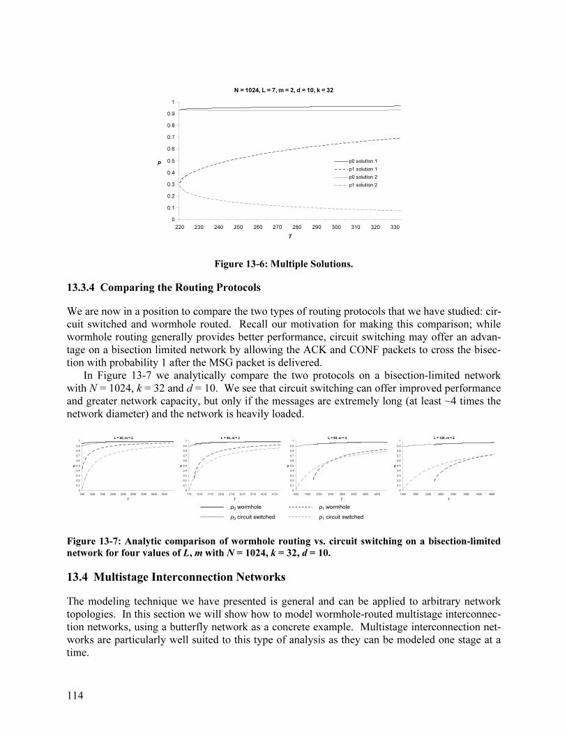
114

N = 1024, L = 7, m = 2, d = 10, k = 32

0

0.1

0.2

0.3

0.4

0.5

0.6

0.7

0.8

0.9

1

220 230 240 250 260 270 280 290 300 310 320 330

T

p p0 solution 1

p1 solution 1

p0 solution 2

p1 solution 2

Figure 13-6: Multiple Solutions.

13.3.4 Comparing the Routing Protocols

We are now in a position to compare the two types of routing protocols that we have studied: cir-

cuit switched and wormhole routed. Recall our motivation for making this comparison; while

wormhole routing generally provides better performance, circuit switching may offer an advan-

tage on a bisection limited network by allowing the ACK and CONF packets to cross the bisec-

tion with probability 1 after the MSG packet is delivered.

In Figure 13-7 we analytically compare the two protocols on a bisection-limited network

with N = 1024, k = 32 and d = 10. We see that circuit switching can offer improved performance

and greater network capacity, but only if the messages are extremely long (at least ~4 times the

network diameter) and the network is heavily loaded.

L = 20, m = 2

0

0.1

0.2

0.3

0.4

0.5

0.6

0.7

0.8

0.9

1

540 1040 1540 2040 2540 3040 3540 4040 4540

T

p

L = 40, m = 3

0

0.1

0.2

0.3

0.4

0.5

0.6

0.7

0.8

0.9

1

710 1210 1710 2210 2710 3210 3710 4210 4710

T

p

L = 80, m = 4

0

0.1

0.2

0.3

0.4

0.5

0.6

0.7

0.8

0.9

1

1050 1550 2050 2550 3050 3550 4050 4550

T

p

L = 120, m = 5

0

0.1

0.2

0.3

0.4

0.5

0.6

0.7

0.8

0.9

1

1390 1890 2390 2890 3390 3890 4390 4890

T

p

Figure 13-7: Analytic comparison of wormhole routing vs. circuit switching on a bisection-limited

network for four values of L, m with N = 1024, k = 32, d = 10.

13.4 Multistage Interconnection Networks

The modeling technique we have presented is general and can be applied to arbitrary network

topologies. In this section we will show how to model wormhole-routed multistage interconnec-

tion networks, using a butterfly network as a concrete example. Multistage interconnection net-

works are particularly well suited to this type of analysis as they can be modeled one stage at a

time.

p0 wormhole

p0 circuit switched

p1 wormhole

p1 circuit switched

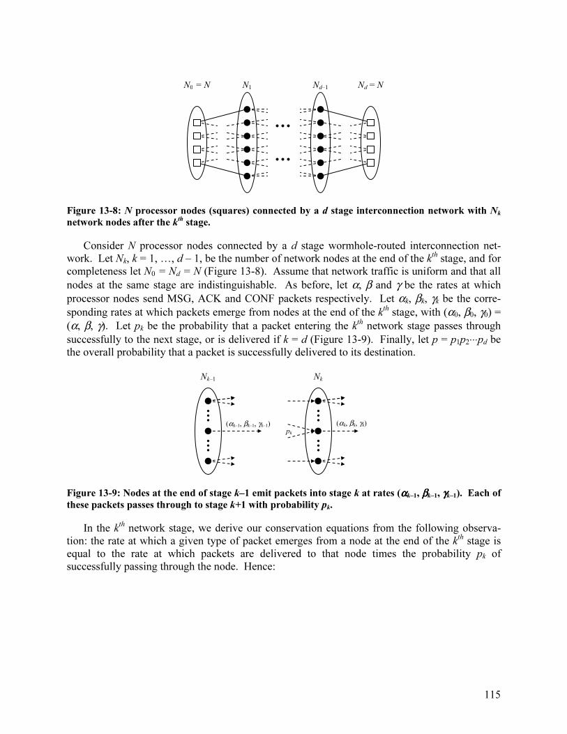
115

Figure 13-8: N processor nodes (squares) connected by a d stage interconnection network with Nk

network nodes after the kth

stage.

Consider N processor nodes connected by a d stage wormhole-routed interconnection net-

work. Let Nk, k = 1, …, d – 1, be the number of network nodes at the end of the kth

stage, and for

completeness let N0 = Nd = N (Figure 13-8). Assume that network traffic is uniform and that all

nodes at the same stage are indistinguishable. As before, let α, β and γ be the rates at which

processor nodes send MSG, ACK and CONF packets respectively. Let αk, βk, γk be the corre-

sponding rates at which packets emerge from nodes at the end of the kth

stage, with (α0, β0, γ0) =

(α, β, γ). Let pk be the probability that a packet entering the kth

network stage passes through

successfully to the next stage, or is delivered if k = d (Figure 13-9). Finally, let p = p1p2⋅⋅⋅pd be

the overall probability that a packet is successfully delivered to its destination.

Figure 13-9: Nodes at the end of stage k–1 emit packets into stage k at rates (ααααk–1, ββββk–1, γγγγk–1). Each of

these packets passes through to stage k+1 with probability pk.

In the kth

network stage, we derive our conservation equations from the following observa-

tion: the rate at which a given type of packet emerges from a node at the end of the kth

stage is

equal to the rate at which packets are delivered to that node times the probability pk of

successfully passing through the node. Hence:

N0 = N N1 Nd–1 Nd = N

(αk–1, βk–1, γk–1)

Nk–1

(αk, βk, γk)

Nk

pk

116

kk

k

k

k

kk

k

k

k

kk

k

k

k

pN

N

pN

N

pN

N

1

1

1

1

1

1

−−

−−

−−

=

=

=

γγ

ββ

αα

(32)

or equivalently,

γγ

ββ

αα

k

kk

k

kk

k

kk

N

Nppp

N

Nppp

N

Nppp

m

m

m

21

21

21

=

=

=

(33)

The port utilization equation for the kth

stage depends on the specific topology of this stage.

Regardless of the topology, the equation will provide a rational expression for pk in terms of αk–1,

βk–1 and γk–1. Finally, the end-to-end conservation equations are the same as equations (5), (8)

and (9). These equations give α, β, γ in terms of p and λ. Using (33) and the port utilization

equations we can inductively find rational expressions for αk, βk, γk and pk in terms of p and λ.

Finally, we can use the end-to-end probability equation p = p1p2⋅⋅⋅pd to solve numerically for p

given λ.

Figure 13-10: 3-state butterfly network.

13.5 Butterfly Network

We now apply the results of the previous section to the butterfly network. A d stage butterfly

network connects N = 2d processor nodes; Figure 13-10 shows a 3-stage butterfly network. Two

features of the butterfly network are relevant to our analysis. First, each stage contains the same

number of nodes, so we can drop the fraction N / Nk from equations (33). Second, the topology

of each stage consists of pairs of nodes at the beginning of the stage which are cross-connected

to the corresponding nodes at the end of the stage. It follows that when a packet is emitted into a

stage, it will be competing with packets from only one other node, but packets are sent to one of

117

two receive ports at the end of the stage depending on their ultimate destination. We therefore

must divide the probability of encountering a busy port by 2, so our port utilization equation for

the kth

stage is

1 – pk = ½ pk(αk–1(L – ½) + (βk–1 + γk–1)(m – ½))

= ½ p1p2⋅⋅⋅ pk(α (L – ½) + (β+ γ)(m – ½)) (34)

Dividing the kth

stage equation by the (k–1)th

stage equation allows us to solve for pk in terms

of pk–1:

11

2

1

1

1

−− −=⇒=

−−

k

kk

k

k

ppp

p

p (35)

If we let pk = ak/bk (where we have a degree of freedom in choosing ak, bk), then equation

(35) becomes:

11

1

2 −−

−

−=

kk

k

k

k

ab

b

b

a (36)

At this point we can use our degree of freedom to assume that the numerators and denomina-

tors of (36) are exactly equal. Thus bk–1 = ak and

ak+1 = 2ak – ak–1 (37)

so {ak} is an arithmetic sequence. Since ad / ad+1 = pd, we can again use the degree of freedom to

assume that ad = pd and ad+1 = 1. It follows that:

ak = pd + (d – k)(pd – 1) (38)

Now the port utilization equation for the dth

stage is:

1 – pd = ½ p(α(L – ½) + (β + γ)(m – ½)) (39)

Using equations (5), (8) and (9) to eliminate α, β and γ, this becomes:

p – p⋅pd = ½(p(2 – p)λ(L – ½) + (1 + p)λ(m – ½)) (40)

Next, we have

d

pp

pdp

a

a

a

a

a

a

a

apppp

d

dd

d

d

d

d

11

1

)1)(1(

1

1

13

2

2

1

21

−+=⇒

−−+==

==

+

+��

(41)

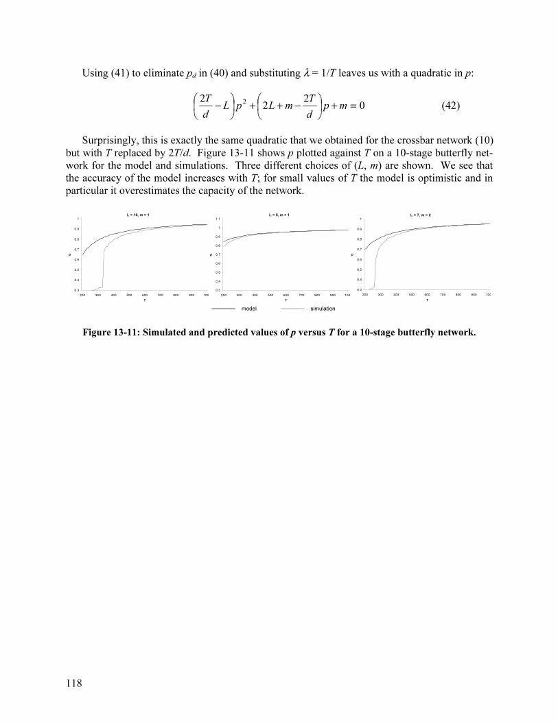
118

Using (41) to eliminate pd in (40) and substituting λ = 1/T leaves us with a quadratic in p:

02

22 2 =+

−++

− mpd

TmLpL

d

T (42)

Surprisingly, this is exactly the same quadratic that we obtained for the crossbar network (10)

but with T replaced by 2T/d. Figure 13-11 shows p plotted against T on a 10-stage butterfly net-

work for the model and simulations. Three different choices of (L, m) are shown. We see that

the accuracy of the model increases with T; for small values of T the model is optimistic and in

particular it overestimates the capacity of the network.

L = 10, m = 1

0.3

0.4

0.5

0.6

0.7

0.8

0.9

1

200 300 400 500 600 700 800 900 100

T

p

L = 5, m = 1

0.3

0.4

0.5

0.6

0.7

0.8

0.9

1

1.1

200 300 400 500 600 700 800 900 100

T

p

L = 7, m = 2

0.3

0.4

0.5

0.6

0.7

0.8

0.9

1

200 300 400 500 600 700 800 900 100

T

p

Figure 13-11: Simulated and predicted values of p versus T for a 10-stage butterfly network.

model simulation

119

Chapter 14

Evaluation of the Idempotent Messaging Protocol

The more we elaborate our means of communication, the less we communicate.

– Joseph Priestley (1733-1804), “Thoughts in the Wilderness”

In this chapter we evaluate the idempotent messaging protocol in simulation. Our simulations

are directed by two specific goals. First, we wish to determine the implementation parameters

that optimize overall performance. Second, we would like to quantify the performance impact of

the messaging protocol compared to wormhole routing on a non-discarding network.

14.1 Simulation Environment

Our evaluations were conducted using a trace-driven network simulator. In this section we de-

scribe the machine model, the format of the traces, how they were obtained, the four micro-

benchmarks that were used, and the parameters of the trace-driven simulator.

14.1.1 Hardware Model

Our hardware model, based on the Hamal architecture, is a distributed shared memory machine

with explicitly split-phase memory operations, hardware multithreading, and register-based syn-

chronization via join capabilities. New threads are created with a fork instruction which speci-

fies the node on which the new thread should run and the set of registers to copy from parent to

child. Memory consistency is enforced in software using a wait instruction. Pointers contain

node and offset fields; distributed objects are implemented by allocating the same range of off-

sets on each node. There are no data caches, which does not affect our results as all micro-

benchmarks explicitly migrate data to where it is needed.

14.1.2 Block Structured Traces

Typically, the input to a trace-driven simulator is simply a set of network messages where each

message specifies a source node, a destination node, the size of the message, and the time at

which the message should be sent. These traces may be obtained by instrumenting actual paral-

lel programs running on multiple real or simulated processor nodes.

There are two problems with this straightforward approach. First, in an actual program the

time at which a given message is sent generally depends on the time that one or more previous

messages were received. It is therefore inaccurate to specify this time a priori in a trace. Sec-

ond, a large parallel computer may not be readily available, and the number of threads required

120

to run a parallel program on thousands of simulated nodes can easily overwhelm the operating

system.

We address the first problem by organizing the trace into blocks of timed messages. Each

block represents a portion of a thread in the parallel program which can execute from start to

finish without waiting for any network messages. When a block is activated, each of its

messages is scheduled to be sent at a specified number of cycles in the future. Each message

optionally specifies a target block to signal when the message is successfully delivered; a block

is activated when it has been signaled by all messages having that block as a target. This block-

structured trace captures the dependency graph of messages within an application, and allows the

simulation to more accurately reflect the pattern of messages that would arise from running the

parallel program with a given network configuration.

Block-structured traces are a similar to intrinsic traces [Holliday92], used in trace-driven

memory simulators to model programs whose address traces depend on the execution environ-

ment. It has been observed that trace-driven parallel program simulations can produce unreliable

results if the traces are of timing-dependent code ([Holliday92], [Goldschmidt93]); our micro-

benchmarks and synchronization mechanisms were therefore chosen to ensure deterministic pro-

gram execution.

14.1.3 Obtaining the Traces

The second problem – the difficulty of simulating thousands of nodes on a single processor – is

addressed by our method of obtaining traces. We provide a small library of routines that imple-

ment the hardware model described in Section 14.1.1; these functions are listed in Table 14-1.

The routines are instrumented to transparently manage threads, blocks, messages, and the pas-

sage of time. Most importantly, they are designed to allow the program to run as a single thread.

This is primarily accomplished by implementing the Fork routine using a function call rather

than actually creating a new thread. Figure 14-1 gives a very simple program written with this

library.

Function Description

Load Load data from a (possibly remote) location

Store Store data to a (possibly remote) location

Wait Wait for all outstanding stores to complete

Fork Start a new thread of execution

Join Write data to another thread’s registers

Sync Register synchronization: wait for a join

Table 14-1: Simulation library functions.

121

void Fork (_thread t, /* thread entry point */int node, /* destination node */...); /* other arguments */

int ComputeSum (Pointer data){

JCap *j = new JCap;Fork(SumThread, 0, numNodes, data, j);return Sync(j);

}

void SumThread (int cNodes, Pointer data, JCap *j){

if (cNodes > 1){

int n = cNodes / 2;JCap *j1 = new JCap;JCap *j2 = new JCap;Fork(SumThread, node, n, data, j1);Fork(SumThread, node + n, cNodes - n, data, j2);Join(j, Sync(j1) + Sync(j2));

}else{

data.node = node;Join(j, Load(data));

}}

Figure 14-1: Sample program to compute the sum of a distributed object with one word on each

node. node and numNodes are global variables.

As an example of how the library routines are implemented, Figure 14-2 gives simplified

code for Load. thread is a global variable managed by the library routines which points to the

current thread of execution. The Load routine begins by creating a new block representing the

continuation of the current thread once the value of the load has been received (it is assumed that

the current thread must wait for this value – we are not taking prefetching into account). Then a

message of type ‘load’ is added to the current block which targets this continuation (the trace

driven simulator automatically generates load reply messages; the target block becomes the tar-

get of the reply). Finally, the thread block pointer is updated to the new block and the contents

of the memory word are returned.

The actual Load routine is slightly more complicated as it also checks for address conflicts

with outstanding stores. The Wait routine is provided to enforce memory consistency by explic-

itly waiting for all stores to complete before execution continues.

While the library routines automatically manage the passage of time for the parallel primi-

tives that they implement, it is the programmer’s job to manage the passage of time for normal

computation. A macro is provided for adding time to the current block. The programmer is re-

sponsible for making use of this macro and providing a reasonable estimate of the number of cy-

cles required to perform a given computation.

122

void Block::AddMessage (int type, /* type of message */int dst, /* destination node */Block *target); /* block to signal */

Word Load (Pointer p){

Block *newBlock = new Block;

thread->block->AddMessage(TYPE_LOAD, p.node, newBlock);thread->block = newBlock;

return memory[p.address];}

Figure 14-2: Load routine (simplified). thread is a global variable.

14.1.4 Synchronization

In the simulation environment, register-based synchronization is accomplished using the Sync

and Join library routines. There are no actual registers in the simulation, so Join is implemented

by storing a word of data in the join capability data structure (and adding a message to the cur-

rent block); Sync retrieves the word from the data structure (and creates a new block).

Because the simulation is run as a single thread, the straightforward implementation of Sync

will only work if the data is already available, i.e. if the corresponding Join has already been

called. If all synchronization is from child to parent then this will always be the case because

implementing Fork using a function call causes the “threads” to run to completion in a depth-first

manner. Figure 14-1 gives an example of child to parent synchronization. While each Fork con-

ceptually creates a new thread, the single-threaded implementation simply calls SumThread as a

subroutine and then returns, so Join will already have been called by the time the parent thread

calls the corresponding Sync.

To allow for more complicated synchronization wherein Sync may be called before the cor-

responding Join, a version of Sync is provided in which the programmer explicitly provides a

continuation. If the data is ready when Sync is called, then the continuation is invoked immedi-

ately. Otherwise the continuation is stored in the join capability data structure and invoked when

the corresponding Join is called (Figure 14-3). This sacrifices some of the transparency of the

simulation environment in order to retain the benefits of being able to run the simulation using a

single thread.

Figure 14-3: (a) Join called before Sync; continuation invoked by Sync. (b) Sync called before

Join; continuation invoked by Join.

parent thread child threads continuation

:Fork(A)

::

Fork(B):

A::

Join()

B::

Sync(C)

C:::::

(a)

:Fork(B)

::

Fork(A):

B::

Sync(C)

A::

Join()

C:::::

(b)

parent thread child threads continuation

123

14.1.5 Micro-Benchmarks

Four micro-benchmarks were chosen to provide a range of network usage patterns. Each one

was coded as described in the previous sections. The four resulting block-structured traces were

used to drive our simulations. The micro-benchmarks are as follows:

add: Parallel prefix addition on 4096 nodes with one word per node. Light network

usage. Network is used for synchronization and thread creation.

reverse: Reverse the data of a 16K entry vector distributed across 1024 nodes. Very heavy

network usage with almost all messages crossing the bisection.

quicksort: Parallel quicksort of a 32K entry random vector on 1024 nodes. Medium, irregu-

lar network usage (lighter than reverse or nbody due to a higher computation to

communication ratio).

nbody: N-body simulation on 256 nodes with one body per node. Computation is struc-

tured for O(√N) communication by conceptually organizing the nodes in a square

array and broadcasting the location of each body to all nodes in the same row and

column. Heavy network usage; network is used in bursts.

14.1.6 Trace-Driven Simulator

The trace driven simulator keeps track of active blocks and memory requests on all nodes in the

system. Blocks are serviced in a round-robin fashion; on each cycle every node picks an active

block and advances it by one time step, possibly generating a new message. This models a mul-

tithreaded processor which is able to issue from a different thread on each cycle. Memory re-

quests are processed on a first-come first-served basis. Each request takes 6 cycles to process,

after which the reply message is automatically generated and the next request can be serviced.

In an attempt to ensure that our results are independent of the network topology, four differ-

ent topologies are used in all simulations: a 2D grid, a 3D grid, a radix-2 dilation-2 multibutter-

fly, and a radix-4 (down) dilation-2 (up) fat tree. For the grid networks dimension-ordered rout-

ing is preferred, but any productive channel may be used to route packets. In all cases wormhole

routing is used, with packet heads advancing one step per cycle. Each network link contains a

small flit buffer; if a packet cannot be advanced due to congestion it may be buffered for as many

cycles as there are flits in the buffer, after which it is discarded. The maximum packet transit

time T is therefore the size of these buffers multiplied by the diameter of the network. When a

node receives an ACK packet it has 32 cycles to respond with a CONF, after which the ACK is

discarded. Receivers must therefore remember messages for 2T + 32 cycles after receiving a

CONF, as explained in Chapter 5.

The size of a packet is determined by the fields that it contains, which in turn is determined

by the packet type. Table 14-2 lists the sizes of the various fields. All fields are fixed-size ex-

cept for the type field which uses a variable length encoding to identify the packet as a CONF, an

ACK, or one of four message types. Table 14-3 lists the sizes of the various packets. In this ta-

ble “MSG header” refers to the four fields present in every message packet which are required to

route the packet and implement the idempotent messaging protocol: type, dest, source and mes-

sage ID. The size of the fork packet depends on the number of registers being copied to the new

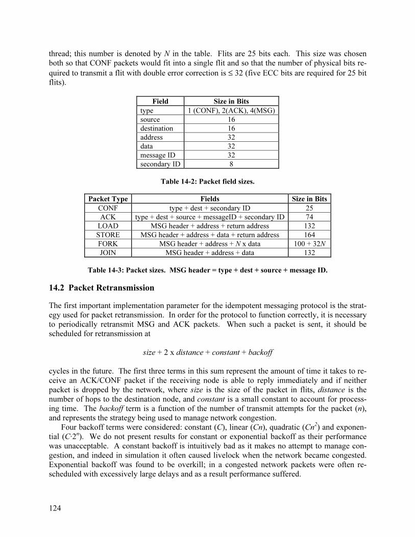
124

thread; this number is denoted by N in the table. Flits are 25 bits each. This size was chosen

both so that CONF packets would fit into a single flit and so that the number of physical bits re-

quired to transmit a flit with double error correction is ≤ 32 (five ECC bits are required for 25 bit

flits).

Field Size in Bits

type 1 (CONF), 2(ACK), 4(MSG)

source 16

destination 16

address 32

data 32

message ID 32

secondary ID 8

Table 14-2: Packet field sizes.

Packet Type Fields Size in Bits

CONF type + dest + secondary ID 25

ACK type + dest + source + messageID + secondary ID 74

LOAD MSG header + address + return address 132

STORE MSG header + address + data + return address 164

FORK MSG header + address + N x data 100 + 32N

JOIN MSG header + address + data 132

Table 14-3: Packet sizes. MSG header = type + dest + source + message ID.

14.2 Packet Retransmission

The first important implementation parameter for the idempotent messaging protocol is the strat-

egy used for packet retransmission. In order for the protocol to function correctly, it is necessary

to periodically retransmit MSG and ACK packets. When such a packet is sent, it should be

scheduled for retransmission at

size + 2 x distance + constant + backoff

cycles in the future. The first three terms in this sum represent the amount of time it takes to re-

ceive an ACK/CONF packet if the receiving node is able to reply immediately and if neither

packet is dropped by the network, where size is the size of the packet in flits, distance is the

number of hops to the destination node, and constant is a small constant to account for process-

ing time. The backoff term is a function of the number of transmit attempts for the packet (n),

and represents the strategy being used to manage network congestion.

Four backoff terms were considered: constant (C), linear (Cn), quadratic (Cn2) and exponen-

tial (C·2n). We do not present results for constant or exponential backoff as their performance

was unacceptable. A constant backoff is intuitively bad as it makes no attempt to manage con-

gestion, and indeed in simulation it often caused livelock when the network became congested.

Exponential backoff was found to be overkill; in a congested network packets were often re-

scheduled with excessively large delays and as a result performance suffered.

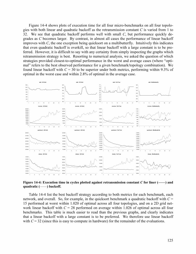
125

Figure 14-4 shows plots of execution time for all four micro-benchmarks on all four topolo-

gies with both linear and quadratic backoff as the retransmission constant C is varied from 1 to

32. We see that quadratic backoff performs well with small C, but performance quickly de-

grades as C becomes larger. By contrast, in almost all cases the performance of linear backoff

improves with C, the one exception being quicksort on a multibutterfly. Intuitively this indicates

that even quadratic backoff is overkill, so that linear backoff with a large constant is to be pre-

ferred. However, it is difficult to say with any certainty from simply inspecting the graphs which

retransmission strategy is best. Resorting to numerical analysis, we asked the question of which

strategies provided closest-to-optimal performance in the worst and average cases (where “opti-

mal” refers to the best observed performance for a given benchmark/topology combination). We

found linear backoff with C = 30 to be superior under both metrics, performing within 9.3% of

optimal in the worst case and within 2.8% of optimal in the average case.

add - 2D Grid

0

200

400

600

800

1000

1200

1400

1 6 11 16 21 26 31

add - 3D Grid

600

650

700

750

800

850

900

1 6 11 16 21 26 31

add - Fat Tree

762

763

764

765

766

767

768

769

770

771

1 6 11 16 21 26 31

add - Multibutterfly

840

860

880

900

920

940

960

1 6 11 16 21 26 31

reverse - 2D Grid

0

20000

40000

60000

80000

100000

120000

140000

160000

180000

200000

1 6 11 16 21 26 31

reverse - 3D Grid

0

5000

10000

15000

20000

25000

30000

35000

1 6 11 16 21 26 31

reverse - Fat Tree

5000

10000

15000

20000

25000

30000

1 6 11 16 21 26 31

reverse - Multibutterfly

800

850

900

950

1000

1050

1100

1150

1200

1 6 11 16 21 26 31

quicksort - 2D Grid

220000

230000

240000

250000

260000

270000

280000

1 6 11 16 21 26 31

quicksort - 3D Grid

170000

175000

180000

185000

190000

195000

200000

1 6 11 16 21 26 31

quicksort - Fat Tree

180000

190000

200000

210000

220000

230000

240000

250000

260000

1 6 11 16 21 26 31

quicksort - Multibutterfly

120000

121000

122000

123000

124000

125000

126000

127000

128000

129000

1 6 11 16 21 26 31

nbody - 2D Grid

100000

105000

110000

115000

120000

125000

130000

135000

1 6 11 16 21 26 31

nbody - 3D Grid

40000

45000

50000

55000

60000

65000

70000

1 6 11 16 21 26 31

nbody - Fat Tree

0

50000

100000

150000

200000

250000

1 6 11 16 21 26 31

nbody - Multibutterfly

30000

35000

40000

45000

50000

55000

1 6 11 16 21 26 31

Figure 14-4: Execution time in cycles plotted against retransmission constant C for liner (––––) and

quadratic (––––) backoff.

Table 14-4 list the best backoff strategy according to both metrics for each benchmark, each

network, and overall. So, for example, in the quicksort benchmark a quadratic backoff with C =

15 performed at worst within 1.020 of optimal across all four topologies, and on a 2D grid net-

work linear backoff with C = 28 performed on average within 1.026 of optimal across all four

benchmarks. This table is much easier to read than the previous graphs, and clearly indicates

that a linear backoff with a large constant is to be preferred. We therefore use linear backoff

with C = 32 (since this is easy to compute in hardware) for the remainder of the evaluations.

126

slowdown over optimal

worst case average case

add 1.009 L5 1.003 L5

reverse 1.028 L30 1.016 L32

quicksort 1.020 Q15 1.015 Q12

nbody 1.085 L31 1.045 L31

2D grid 1.033 L32 1.026 L28

3D grid 1.039 L32 1.018 L30

fat tree 1.085 L31 1.036 L30

multibutterfly 1.041 L32 1.015 L32

overall 1.093 L30 1.028 L30

Table 14-4: Best backoff strategy as measured by worst case and average case slowdown over opti-

mal for each benchmark, each network, and overall.

It is worth noting that our results differ from those obtained in [Brown02b]. Our simulations

and analyses have changed in three respects. First, the simulator has been improved to more ac-

curately model threads and memory references. Second, flit buffering has been added to the

network nodes. Third, the multibutterfly network has been included in the simulations. The

graphs of Figure 14-4 are qualitatively similar to those in [Brown02b], but numerical analysis

has yielded different results.

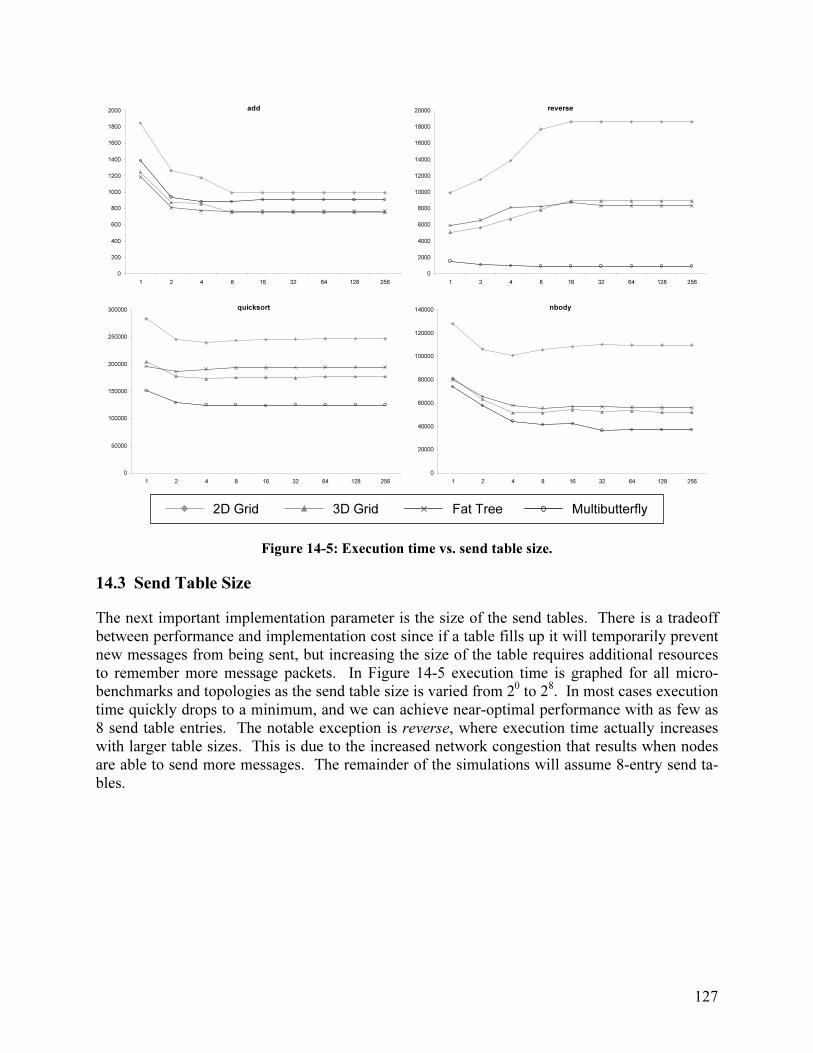
127

add

0

200

400

600

800

1000

1200

1400

1600

1800

2000

1 2 4 8 16 32 64 128 256

reverse

0

2000

4000

6000

8000

10000

12000

14000

16000

18000

20000

1 2 4 8 16 32 64 128 256

quicksort

0

50000

100000

150000

200000

250000

300000

1 2 4 8 16 32 64 128 256

nbody

0

20000

40000

60000

80000

100000

120000

140000

1 2 4 8 16 32 64 128 256

Figure 14-5: Execution time vs. send table size.

14.3 Send Table Size

The next important implementation parameter is the size of the send tables. There is a tradeoff

between performance and implementation cost since if a table fills up it will temporarily prevent

new messages from being sent, but increasing the size of the table requires additional resources

to remember more message packets. In Figure 14-5 execution time is graphed for all micro-

benchmarks and topologies as the send table size is varied from 20 to 2

8. In most cases execution

time quickly drops to a minimum, and we can achieve near-optimal performance with as few as

8 send table entries. The notable exception is reverse, where execution time actually increases

with larger table sizes. This is due to the increased network congestion that results when nodes

are able to send more messages. The remainder of the simulations will assume 8-entry send ta-

bles.

2D Grid 3D Grid Fat Tree Multibutterfly

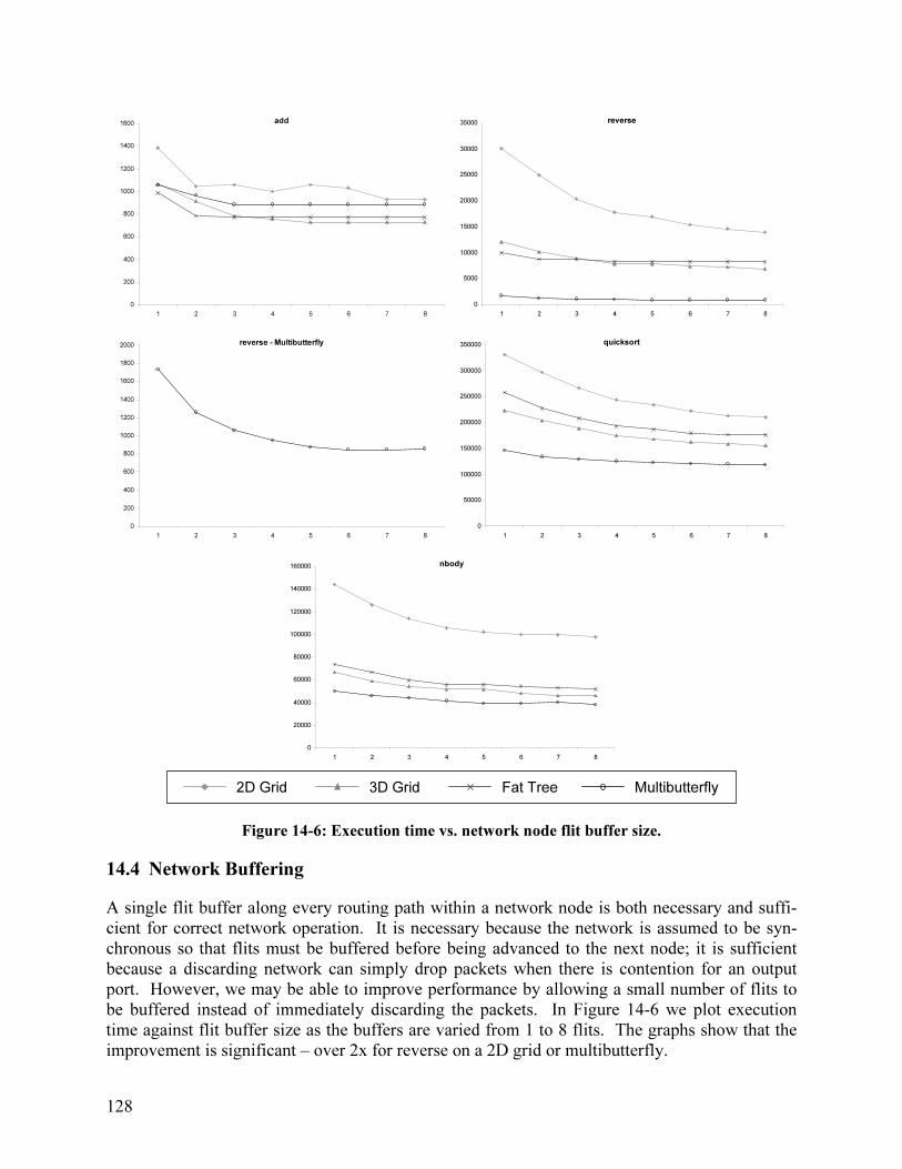
128

add

0

200

400

600

800

1000

1200

1400

1600

1 2 3 4 5 6 7 8

reverse

0

5000

10000

15000

20000

25000

30000

35000

1 2 3 4 5 6 7 8

reverse - Multibutterfly

0

200

400

600

800

1000

1200

1400

1600

1800

2000

1 2 3 4 5 6 7 8

quicksort

0

50000

100000

150000

200000

250000

300000

350000

1 2 3 4 5 6 7 8

nbody

0

20000

40000

60000

80000

100000

120000

140000

160000

1 2 3 4 5 6 7 8

Figure 14-6: Execution time vs. network node flit buffer size.

14.4 Network Buffering

A single flit buffer along every routing path within a network node is both necessary and suffi-

cient for correct network operation. It is necessary because the network is assumed to be syn-

chronous so that flits must be buffered before being advanced to the next node; it is sufficient

because a discarding network can simply drop packets when there is contention for an output

port. However, we may be able to improve performance by allowing a small number of flits to

be buffered instead of immediately discarding the packets. In Figure 14-6 we plot execution

time against flit buffer size as the buffers are varied from 1 to 8 flits. The graphs show that the

improvement is significant – over 2x for reverse on a 2D grid or multibutterfly.

2D Grid 3D Grid Fat Tree Multibutterfly

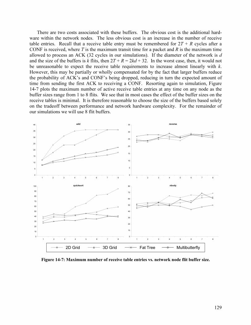
129

There are two costs associated with these buffers. The obvious cost is the additional hard-

ware within the network nodes. The less obvious cost is an increase in the number of receive

table entries. Recall that a receive table entry must be remembered for 2T + R cycles after a

CONF is received, where T is the maximum transit time for a packet and R is the maximum time

allowed to process an ACK (32 cycles in our simulations). If the diameter of the network is d

and the size of the buffers is k flits, then 2T + R = 2kd + 32. In the worst case, then, it would not

be unreasonable to expect the receive table requirements to increase almost linearly with k.

However, this may be partially or wholly compensated for by the fact that larger buffers reduce

the probability of ACK’s and CONF’s being dropped, reducing in turn the expected amount of

time from sending the first ACK to receiving a CONF. Resorting again to simulation, Figure

14-7 plots the maximum number of active receive table entries at any time on any node as the

buffer sizes range from 1 to 8 flits. We see that in most cases the effect of the buffer sizes on the

receive tables is minimal. It is therefore reasonable to choose the size of the buffers based solely

on the tradeoff between performance and network hardware complexity. For the remainder of

our simulations we will use 8 flit buffers.

add

0

5

10

15

20

25

30

35

40

1 2 3 4 5 6 7 8

reverse

0

5

10

15

20

25

30

35

1 2 3 4 5 6 7 8

quicksort

0

10

20

30

40

50

60

70

80

90

100

1 2 3 4 5 6 7 8

nbody

0

10

20

30

40

50

60

70

80

1 2 3 4 5 6 7 8

Figure 14-7: Maximum number of receive table entries vs. network node flit buffer size.

2D Grid 3D Grid Fat Tree Multibutterfly

130

add

0

500

1000

1500

2000

2500

3000

3500

16 32 64 128

reverse

0

2000

4000

6000

8000

10000

12000

14000

16000

16 32 64 128

quicksort

0

50000

100000

150000

200000

250000

300000

16 32 64 128

nbody

0

20000

40000

60000

80000

100000

120000

140000

16 32 64 128

Figure 14-8: Execution time vs. receive table size.

14.5 Receive Table Size

If a receive table fills, new message packets which arrive over the network must be dropped.

This wastes network bandwidth since these packets have already traversed the network, so it is

important to ensure that the receive tables are not too small. At the same time there are two costs

associated with the receive tables. First, the tables themselves require expensive content-

addressable memory. Second, the size of the secondary ID’s is the base 2 logarithm of the re-

ceive table size (recall that a secondary ID is a direct index into the receive table). Thus, increas-

ing the size of the receive tables beyond a power of two increases the size of both ACK and

CONF packets.

In Figure 14-8 execution time is plotted against four different receive table sizes (16, 32, 64,

128). We see a significant improvement in performance from 16 to 32 entries, moderate im-

provement from 32 to 64 entries, and negligible improvement from 64 to 128 entries. As can be

seen from Figure 14-7, this is largely due to the fact that most benchmark/topology combinations

never use more than 64 receive table entries in the worst case. Figure 14-8 shows that in the

cases where more than 64 entries are required, performance is barely affected by limiting the size

of the receive table to 64. We therefore use 64-entry receive tables for the remainder of the

simulations. Note that this reduces the size of CONF packets to 23 bits and the size of ACK

packets to 72 bits.

2D Grid 3D Grid Fat Tree Multibutterfly

131

add

0

200

400

600

800

1000

1200

1400

16 17 18 19 20 21 22 23 24 25 26 27 28 29 30 31 32

reverse

0

5000

10000

15000

20000

25000

30000

35000

40000

16 17 18 19 20 21 22 23 24 25 26 27 28 29 30 31 32

reverse - multibutterfly

0

200

400

600

800

1000

1200

1400

16 17 18 19 20 21 22 23 24 25 26 27 28 29 30 31 32

quicksort

0

50000

100000

150000

200000

250000

300000

350000

16 17 18 19 20 21 22 23 24 25 26 27 28 29 30 31 32

nbody

0

20000

40000

60000

80000

100000

120000

140000

160000

180000

200000

16 17 18 19 20 21 22 23 24 25 26 27 28 29 30 31 32

Figure 14-9: Execution time vs. channel width.

14.6 Channel Width

Different network implementations will make use of different flit sizes. In Figure 14-9 we show

execution time plotted against flit size as the number of bits in a flit varies from 16 to 32. We

see that our choice of 25 bit flits was fortuitous; there is a significant improvement in perform-

ance from 16 to 25 bits, but little improvement beyond that point. Figure 14-10 provides some

intuition for these graphs by showing packet size vs. flit size for five different packet types. Fork

(3) refers to a fork packet where 3 registers are copied into the child thread. Note that for many

benchmark/topology combinations there is a noticeable improvement in performance from 23

2D Grid 3D Grid Fat Tree Multibutterfly

132

bits to 24 bits as the size of the ACK packets drops from 4 flits to 3 flits (e.g. reverse on a 2D

grid).

Packet Size

0

2

4

6

8

10

12

14

16 17 18 19 20 21 22 23 24 25 26 27 28 29 30 31 32

flit size (bits)

packet

siz

e (

flit

s)

Load

Store

Fork (3)

ACK

CONF

Figure 14-10: Packet size in flits vs. flit size in bits.

14.7 Performance Comparison: Discarding vs. Non-Discarding

For small systems it is probably worth constructing a reliable network, whereas for extremely

large systems it is almost certainly necessary to implement a fault-tolerant messaging protocol.

In between these extremes, however, it may be difficult to determine which approach is more

appropriate, and it becomes useful to know the performance impact of the fault-tolerant

messaging protocol.

To compare the two approaches, we simulated a perfect network with both the discarding

protocol and non-discarding buffered wormhole routing. In both cases network nodes have 8-

entry flit buffers and each communication link consists of 30 physical bits. In the discarding

network 25 of these bits contain data and 5 are ECC bits required to detect up to two bit errors.

In the non-discarding network, errors must be corrected, not simply detected, which requires 9

bits. Additionally, a single backpressure bit is required to prevent buffer overruns. Thus, the

non-discarding network uses 20 bit flits. For the non-discarding grid networks, strict dimension-

ordered routing is used to avoid deadlocks [Dally87].

The results of the comparison are shown in Table 14-5. We see that the actual slowdown,

which ranges from as little as 0.99 to as much as 3.36, depends on both the application and the

network topology. In general, a more congested network leads to greater slowdowns. Note that

in our simulations we are assuming that the cycle times of the two networks are the same. In

practice this would likely not be the case for two reasons. First, the control logic of the discard-

ing network is much simpler than that of the non-discarding network; as a result it will be possi-

ble to clock the discarding network nodes at a higher speed ([DeHon94], [Chien98]). Second,

with a fault-tolerant messaging protocol it is possible to boost the clock speed even further since

one does not need to worry about introducing the occasional signaling error so long as it can be

detected.

133

2D Grid 3D Grid Fat Tree Multibutterfly

discarding? discarding? discarding? discarding?

topology:

no yes

slow-

down no yes

slow-

down no yes

slow-

down no yes

slow-

down

add 934 926 0.99 741 730 0.99 773 768 0.99 893 884 0.99

reverse 4711 13924 2.96 2372 6829 2.88 2432 8183 3.36 640 859 1.34

quicksort 165368 212296 1.28 128526 155849 1.21 119382 176369 1.48 110543 118979 1.08

nbody 44200 98708 2.23 33576 45838 1.37 36115 51930 1.44 34369 38146 1.11

Table 14-5: Slowdown of messaging protocol compared to wormhole routing on a perfect network.

We can attempt to quantify the amount by which clock speed may be increased by “normal-

izing for reliability”, that is, choosing network parameters so that both the discarding and the

non-discarding networks have the same mean time between failures (MTBF). Suppose we wish

the network as a whole to have a MTBF of 1010

seconds. Assuming a 1GHz network, this is 1019

cycles. If ~105 flits are transferred on each cycle, then the probability of failure for a single flit

should be 10-24

.

In the non-discarding network, each flit consists of 29 bits, including ECC bits. A failure oc-

curs whenever a flit contains 3 or more single bit errors. If the probability of error for a single

bit is p, then to first order the probability of failure for the entire flit is

333654

3

29pp =

(1)

⇒ 3654 p3 = 10

-24 ⇒ p ≈ 6.492 x 10

-10. Next we must relate p to the clock speed. We will

consider the case in which sampling jitter is the dominant source of error, where by “sampling

jitter” we mean the combination of signal jitter and receiver clock jitter. Assume that signal

setup time t and sampling jitter j are fixed by the physical interconnect, circuit design and fabri-

cation process, independent of clock speed. Assume further that the sampling jitter j is normally

distributed [Kleeman90]. If the clock has period T, then the probability of a bit error is

−>22

1 tTjP (2)

This equation assumes that if the signal is sampled within the sampling window of size T – t

then the correct value is obtained, otherwise a random value is obtained so that the probability of

error is ½. Figure 14-11 illustrates the model we are using.

Figure 14-11: Normally distributed sampling jitter.

t

T

window

signal

jitter

134

The probability p can be determined by measuring the width of the sampling window in

standard deviations δ of j. Using (1) and (2) we find ½(T – t) ≈ 6.068δ.

To properly trade off speed for reliability in the discarding network, we use 6 ECC bits and

24 data bits to allow for up to three single bit errors. In Chapter 4, Section 4.6.4 we observed

that a linear code has d ≥ 4 if the columns of its parity check matrix are distinct and have odd

weight. We can therefore define a (30, 24, 4) linear code by constructing its 6x30 parity check

matrix: fill the columns of the upper 5x30 submatrix with all five-bit binary integers except for

00000 and 11111, then fill in the bottom row so that each column has odd weight (Figure 14-12).

0 0 0 0 0 0 0 0 0 0 0 0 0 0 0 1 1 1 1 1 1 1 1 1 1 1 1 1 1 1 0 0 0 0 0 0 0 1 1 1 1 1 1 1 1 0 0 0 0 0 0 0 0 1 1 1 1 1 1 1 0 0 0 1 1 1 1 0 0 0 0 1 1 1 1 0 0 0 0 1 1 1 1 0 0 0 0 1 1 1 0 1 1 0 0 1 1 0 0 1 1 0 0 1 1 0 0 1 1 0 0 1 1 0 0 1 1 0 0 1 1 0 1 0 1 0 1 0 1 0 1 0 1 0 1 0 1 0 1 0 1 0 1 0 1 0 1 0 1 0 0 0 1 0 1 1 0 0 1 1 0 1 0 0 1 0 1 1 0 1 0 0 1 1 0 0 1 0 1 1

Figure 14-12: Parity check matrix for a (30, 24, 4) linear code.

In the discarding network, a failure is an undetected error. Thus, a failure occurs whenever a

flit contains 4 or more single bit errors and the modified flit is a valid code word. Since we are

using a linear code, this is the case if and only if the error vector itself is a valid code word. It

can be shown using a simple counting argument (or by brute force if one is not inclined to count)

that the given code contains 945 code words of weight 4. Thus, if the probability of error for a

single bit is p, then to first order the probability of failure for an entire flit is 945 p4 ⇒ 945 p

4 =

10-24

⇒ p ≈ 1.804 x 10-7

. If the clock period in the discarding network is T’, then in this case

we find ½(T’ – t) ≈ 5.089δ.

Finally, to relate the clock speeds of the two networks we must make an additional assump-

tion regarding the size of the sampling window relative to the clock period. Assuming that t =

T/3, we have

TTTTTTTT

892.0332068.6

089.5'

089.5

3'

068.6

3 ≈+=⇒−=−

(3)

If we again compare the two approaches under the assumption that the non-discarding net-

work has 24 bit flits and a clock that runs 11% faster, we obtain the results shown in Table 14-6.

In this case the slowdowns are slightly less severe.

2D Grid 3D Grid Fat Tree Multibutterfly

discarding? discarding? discarding? discarding?

topology:

no yes

slow-

down no yes

slow-

down no yes

slow-

down no yes

slow-

down

add 934 862 0.92 741 690 0.93 773 722 0.93 893 825 0.92

reverse 4711 13765 2.92 2372 7007 2.95 2432 7809 3.21 640 845 1.32

quicksort 165368 200076 1.21 128526 148210 1.15 119382 165556 1.39 110543 112669 1.02

nbody 44200 91019 2.06 33576 43378 1.29 36115 49989 1.38 34369 35319 1.03

Table 14-6: Slowdown when discarding network uses 24 bit flits and runs 11% faster.

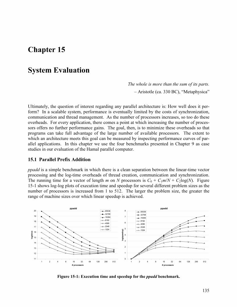
135

Chapter 15

System Evaluation

The whole is more than the sum of its parts.

– Aristotle (ca. 330 BC), “Metaphysica”

Ultimately, the question of interest regarding any parallel architecture is: How well does it per-

form? In a scalable system, performance is eventually limited by the costs of synchronization,

communication and thread management. As the number of processors increases, so too do these

overheads. For every application, there comes a point at which increasing the number of proces-

sors offers no further performance gains. The goal, then, is to minimize these overheads so that

programs can take full advantage of the large number of available processors. The extent to

which an architecture meets this goal can be measured by inspecting performance curves of par-

allel applications. In this chapter we use the four benchmarks presented in Chapter 9 as case

studies in our evaluation of the Hamal parallel computer.

15.1 Parallel Prefix Addition

ppadd is a simple benchmark in which there is a clean separation between the linear-time vector

processing and the log-time overheads of thread creation, communication and synchronization.

The running time for a vector of length m on N processors is C0 + C1m/N + C2log(N). Figure

15-1 shows log-log plots of execution time and speedup for several different problem sizes as the

number of processors is increased from 1 to 512. The larger the problem size, the greater the

range of machine sizes over which linear speedup is achieved.

ppadd

11

12

13

14

15

16

17

18

19

20

1 2 4 8 16 32 64 128 256 512

# processors

log(tim

e)

65536

32768

16384

8192

4096

2048

1024

ppadd

0

1

2

3

4

5

6

7

8

1 2 4 8 16 32 64 128 256 512

# processors

log(speedup)

65536

32768

16384

8192

4096

2048

1024

Figure 15-1: Execution time and speedup for the ppadd benchmark.

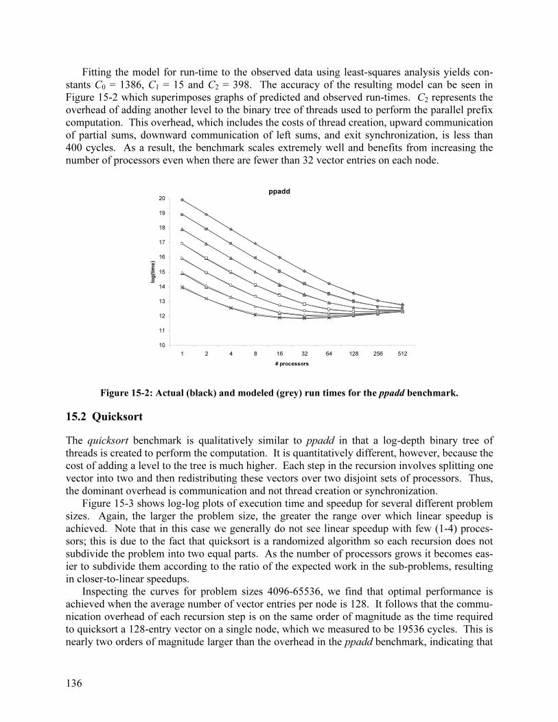
136

Fitting the model for run-time to the observed data using least-squares analysis yields con-

stants C0 = 1386, C1 = 15 and C2 = 398. The accuracy of the resulting model can be seen in

Figure 15-2 which superimposes graphs of predicted and observed run-times. C2 represents the

overhead of adding another level to the binary tree of threads used to perform the parallel prefix

computation. This overhead, which includes the costs of thread creation, upward communication

of partial sums, downward communication of left sums, and exit synchronization, is less than

400 cycles. As a result, the benchmark scales extremely well and benefits from increasing the

number of processors even when there are fewer than 32 vector entries on each node.

ppadd

10

11

12

13

14

15

16

17

18

19

20

1 2 4 8 16 32 64 128 256 512

# processors

log(tim

e)

Figure 15-2: Actual (black) and modeled (grey) run times for the ppadd benchmark.

15.2 Quicksort

The quicksort benchmark is qualitatively similar to ppadd in that a log-depth binary tree of

threads is created to perform the computation. It is quantitatively different, however, because the

cost of adding a level to the tree is much higher. Each step in the recursion involves splitting one

vector into two and then redistributing these vectors over two disjoint sets of processors. Thus,

the dominant overhead is communication and not thread creation or synchronization.

Figure 15-3 shows log-log plots of execution time and speedup for several different problem

sizes. Again, the larger the problem size, the greater the range over which linear speedup is

achieved. Note that in this case we generally do not see linear speedup with few (1-4) proces-

sors; this is due to the fact that quicksort is a randomized algorithm so each recursion does not

subdivide the problem into two equal parts. As the number of processors grows it becomes eas-

ier to subdivide them according to the ratio of the expected work in the sub-problems, resulting

in closer-to-linear speedups.

Inspecting the curves for problem sizes 4096-65536, we find that optimal performance is

achieved when the average number of vector entries per node is 128. It follows that the commu-

nication overhead of each recursion step is on the same order of magnitude as the time required

to quicksort a 128-entry vector on a single node, which we measured to be 19536 cycles. This is

nearly two orders of magnitude larger than the overhead in the ppadd benchmark, indicating that

137

while the Hamal architecture provides extremely efficient thread management and synchroniza-

tion, communication is an area of weakness.

quicksort

17

18

19

20

21

22

23

24

25

26

27

1 2 4 8 16 32 64 128 256 512

# processors

log(tim

e)

262144

131072

65536

32768

16384

8192

4096

quicksort

0

1

2

3

4

5

6

7

1 2 4 8 16 32 64 128 256 512

# processors

log(speedup)

262144

131072

65536

32768

16384

8192

4096

Figure 15-3: Execution time and speedup for the quicksort benchmark.

15.3 N-body Simulation

The nbody benchmark has been optimized for communication by conceptually arranging the

processor nodes in a square array; processors communicate only with other processors in the

same row or column. With m bodies distributed across N processors, each processor maintains

m/N bodies and must send them to (2√N – 1) other processors, and each processor computes and

communicates a partial force for each of the m/√N bodies in its row, so the communication over-

head is proportional to m/√N. Each processor must then compute the force interactions between

the m/√N bodies in its row and the m/√N in its column, so the work for each processor is propor-

tional to m2/N. Furthermore, the constant for this work is fairly high since each force interaction

requires performing the computation

( )232

12

2

12

2

12

121212

)()()(

),,(

zzyyxx

zzyyxxm

−+−+−

−−−

We measured this constant to be approximately 70 cycles. Roughly speaking, we expect per-

formance to improve as the number of nodes is increased as long as the communication overhead

is less than the single-threaded workload, i.e. Cm/√N < 70m2/N where C is the constant for the

communication overhead. Simplifying, this condition becomes N < (70m/C)2. From this we see

that nbody is extremely scalable and, indeed, the execution time and speedup curves for 256 bod-

ies on 1-256 processors (Figure 15-4) are almost perfectly linear. This is an indication that 256

<< (70⋅256/C)2, so C << 1120. Thus, the average cost of communicating 2 bodies and 1 force (a

total of 88 bytes, using double-precision floating point numbers) in a 256 node machine is much

less than 1120 cycles. This is not terribly informative and merely serves to reassure us that while

the performance of communication in the Hamal architecture is not optimal, neither is it unac-

ceptable.

138

nbody

17

18

19

20

21

22

23

24

25

26

1 2 3 4 5

# processors

log(tim

e)

nbody

0

2

4

6

8

1 4 16 64 256

# processors

log(speedup)

Figure 15-4: Execution time and speedup for the nbody benchmark.

15.4 Wordcount

The wordcount benchmark differs from the other three in that commonly occurring words (such

as ‘a’ and ‘the’) introduce sequential bottlenecks which constrain performance as the number of

processors is increased. Figure 15-5 shows execution time and speedup for the best-performing

version of the program, which is a spin-waiting local-access version in which each parent thread

creates at most one child thread at a time. For ≤ 16 processors there is no lock contention, and as

a result good speedups are observed. The speedup is slightly less than linear due primarily to

load imbalance (each child thread is essentially created on a random node depending on the hash

value of the current word). At 32 processors we see the emergence of contention which noticea-

bly impacts performance. Additionally, the sequential bottlenecks start to become significant.

Thereafter, performance improves at a much reduced rate.

From an evaluation standpoint, the most significant aspect of the wordcount benchmark is the

large number of threads that it generates (over 30,000 – one for every word in [Brown02b]).

This demonstrates the effectiveness of the thread management mechanisms in the Hamal proces-

sor and microkernel. In particular, the low cost of remote thread creation gives rise to the speed-

ups observed with ≤ 16 processors.

wordcount

0

1

2

3

4

5

6

1 2 4 8 16 32 64 128 256 512

# processors

tim

e (

millio

ns o

f cycle

s)

wordcount

0

1

2

3

4

1 2 4 8 16 32 64 128 256 512

# processors

log(speedup)

Figure 15-5: Execution time and speedup for the wordcount benchmark.

139

15.5 Multiprogramming

Hamal is a general purpose architecture and is designed to provide efficient support for running

multiple independent programs via hardware multithreading and low-overhead thread manage-

ment. Processor utilization is maximized by dynamically choosing a context to issue on every

cycle, allowing concurrent threads to fill each other’s pipeline bubbles and memory stalls.

Figure 15-6 shows execution times and processor utilization for various combinations of the

quicksort and nbody benchmarks run concurrently on 16 processors. quicksort was run on a 216

entry vector, and nbody was run for 10 iterations; these parameters were chosen to roughly

equalize the run-times of the individual benchmarks. Figure 15-6 graphs total numbers of

processor cycles (there are 16 processor cycles on each machine cycle) and breaks them down

into three categories. On a given processor, a cycle is a program cycle if a user thread issues, a

kernel cycle if the kernel running in context 0 issues, and an unused cycle if no context can issue.

The first two bars of Figure 15-6a give execution times for quicksort and nbody run on their own.

The remaining bars given execution times for concurrent execution of copies of these bench-

marks, using the nomenclature qXnY for X copies of quicksort and Y copies of nbody. Data is

collected from the time the machine boots to the time the last user thread exits.

Both graphs clearly illustrate the benefits of cycle-by-cycle multithreading which results in

sub-additive run-times (Figure 15-6a) and increased processor utilization (Figure 15-6b). The

execution time of q1b1 is only slightly greater than that of the benchmarks run alone; in general

program cycles are almost exactly additive whereas the number of unused cycles decreases.

Note that as the number of threads increases, so too does the number of kernel cycles as more

work is required to manage these threads. However, the kernel is largely able to take advantage

of otherwise unused cycles so this has little effect on the overall run time (compare the number

of kernel and unused cycles for q3n2 and q3n3).

multiprogrammed workload

0

20

40

60

80

100

120

140

160

quicksort nbody q1n1 q2n1 q1n2 q2n2 q3n2 q2n3 q3n3

ex

ec

uti

on

tim

e (

mil

lio

ns

of

pro

ce

ss

or

cy

cle

s)

unused cycles

kernel cycles

program cycles

multiprogrammed workload

0%

10%

20%

30%

40%

50%

60%

70%

80%

90%

100%

quicksort nbody q1n1 q2n1 q1n2 q2n2 q3n2 q2n3 q3n3

pro

ce

ss

or

uti

liza

tio

n

(a) (b)

Figure 15-6: (a) Execution time and (b) processor utilization for concurrent execution of the quick-

sort and nbody benchmarks.

15.6 Discussion

Without question, the main strength of the Hamal architecture lies in its broad support for mas-

sive fine-grained parallelism. The low overheads of thread creation, concurrent execution, con-

text swapping, event-driven thread management and register-based synchronization allow paral-

lel applications to obtain high speedups as the number of processors is increased. The efficiency

140

of thread management permits the use of a large number of threads without overwhelming the

system (there are over 30,000 threads in wordcount and over 50,000 in quicksort on 512 nodes).

Communication, on the other hand, is an area of weakness. In particular, possibly the most seri-

ous design flaw in the Hamal architecture is the lack of hardware support for data streaming. In

order to move data from one node to another an application must write it to remote memory 128

bits at a time. Each write is placed in a separate network packet, incurring an overhead of at

least 300%. This simple method of communication is sufficient for processor-intensive applica-

tions such as nbody, but noticeably impacts both the performance and potential scalability of

communication-intensive applications such as quicksort.

141

Chapter 16

Conclusions and Future Work

Great is the art of beginning, but greater is the art of ending.

– Henry Wadsworth Longfellow (1807-82)

The goal of a building a general-purpose shared-memory machine with millions or even billions

of nodes gives rise to a number of design challenges and requires fundamental changes to the

models currently used to construct systems with hundreds or thousands of processors. Ulti-

mately, success will depend on advances in fabrication technology, computer architecture, fault

management, compilers, programming languages, and development environments. This thesis

has focused on hardware design, and we have presented Hamal: a shared-memory architecture

with efficient support for massive parallelism which is directly scalable to one million nodes. In

this chapter we summarize the key features of Hamal as well as our major findings, and we sug-

gest directions for further research.

16.1 Memory System

A memory system is the canvas on which a parallel architecture is painted. A properly designed

memory system facilitates the creation of a flexible and easily programmable machine, whereas a

poor design inhibits performance and limits scalability. The Hamal memory system addresses

the needs of future architectures by tightly integrating processors with memory and by making

use of mechanisms which support arbitrary scaling.

The basic building block of the Hamal memory system is the capability, a tagged, unforge-

able pointer containing hardware-enforced permissions and segment bounds. The use of capa-

bilities has two important consequences. First, they allow the use of a single shared virtual ad-

dress space. This greatly reduces the amount of state associated with a process and allows data

to be shared simply by communicating a pointer. Second, capabilities ensure that all memory

references are valid. Page faults no longer require the operating system to validate the faulting

address, and they can be used to implement lazy allocation of physical pages. Additionally, we

have seen that it can be useful to place auxiliary information within the capability: we presented

squids, which allow an architecture to support forwarding pointers without the overhead nor-

mally associated with aliasing problems.

All memory operations are explicitly split-phased, and a thread may continue to perform

computation while it is waiting for replies from one or more memory requests. The hardware

does not enforce any consistency model and makes no guarantee regarding the order in which

memory operations with different addresses complete; weak consistency is supported via a wait

instruction which allows software to wait for all outstanding memory operations to complete.

142

Virtual memory is implemented using a fixed mapping from virtual addresses to physical

nodes and with associative hardware page tables, located at the memory, to perform virtual→

physical address translation. This completely eliminates the need for translation lookaside buff-

ers, simplifying processor design and removing an obstacle to scalability.

We have presented extended address partitioning as well as an implementation of sparsely

faceted arrays [Brown02b]. Each of these mechanisms allows distributed objects to be atomi-

cally allocated by a single node without any global communication or synchronization. Physical

storage for distributed objects is lazily allocated on demand in response to page faults. A hard-

ware swizzle instruction is provided to allow applications to map a continuous range of indices to

addresses within a distributed object in a flexible manner.

16.2 Fault-Tolerant Messaging Protocol

In a machine with millions of discrete network components, it is extremely difficult to prevent

electrical or mechanical failures from corrupting packets within the network. In the future, sys-

tems will need to rely on end-to-end messaging protocols in order to guarantee packet delivery.

We have presented an implementation of a lightweight fault-tolerant messaging protocol

[Brown02a] which ensures both message delivery and message idempotence. Each communica-

tion is broken down into three parts: a message, an acknowledgement which indicates message

reception, and a confirmation which indicates that the message will not be re-sent. The protocol

does not require global information to be stored at each node and is therefore inherently scalable.

We have shown how the overhead of this protocol can be reduced by using receiver-generated

secondary ID’s.

We have developed an analytical model using a technique that can be applied to any fault-

tolerant messaging protocol. The accuracy of the model was verified by simulation. An evalua-

tion of the messaging protocol was conducted using block-structured trace driven simulations.

We found that performance is optimized with small send tables (~8 entries), slightly larger re-

ceive tables (~64 entries), and with linear backoff used for packet retransmission.

16.3 Thread Management

Massive parallelism implies massive multithreading; a scalable machine must be able to effec-

tively manage a large number of threads. Hamal contains a number of mechanisms to minimize

the overhead of thread management. A multithreaded processor allows multiple threads to exe-

cute concurrently. New threads are created using a single fork instruction which specifies a start-

ing address for the new thread, the node on which the thread is to be created, and the set of gen-

eral-purpose registers which are to be copied into the thread. Nodes contain 8-entry fork queues

from which new threads can be loaded directly into a context or stored to memory for later acti-

vation. Each thread is associated with a hardware-recognized swap page in memory; this pro-

vides a uniform naming mechanism for threads and enables the use of register-dribbling to load

and unload contexts in the background. Finally, stall events inform the microkernel that a con-

text is unable to issue, allowing rapid replacement of blocked threads.

The effectiveness of these mechanisms was experimentally confirmed by simulating a num-

ber of parallel benchmark programs. Good speedups were observed, and benchmarks were able

to make use of a large number of threads (over 50,000 in quicksort) without overwhelming the

system. Additionally, cycle-by-cycle hardware multithreading was found to provide efficient

support for mutiprogrammed workloads by significantly increasing processor utilization.

143

16.4 Synchronization

Typically, the threads of a parallel program do not run in isolation; they collaborate to perform a

larger task. Synchronization is required to ensure correctness by enforcing data dependencies

and protecting the integrity of shared data structures. Hamal provides four different synchroniza-

tion primitives. Atomic memory operations are the atomic read-and-modify operations found in

all modern architectures. Shared registers provide efficient support for brief periods of mutual

exclusion while accessing heavily-used shared data such as the malloc counter. Register-based

synchronization allows one thread to write directly to another thread’s registers, giving synchro-

nization the same semantics and overheads as a high-latency memory operation. Register-based

synchronization can be used to implement fast barrier and exit synchronization; the latency of a

software barrier on 512 nodes is only 523 cycles. Finally, UV trap bits extend the semantics of

memory operations in a flexible manner and can be used to implement a number of high-level

synchronization primitives including locks and producer-consumer structures. Our experiments

confirmed the results reported in [Kranz92] regarding the performance advantages of using trap

bits in memory to implement fine-grained synchronization. Additionally, we found the primary

advantage of Hamal’s UV trapping mechanism over previous similar mechanisms to be the han-

dling of traps on the node containing the memory word rather than on the node which initiated

the memory request.

16.5 Improving the Design

Our experience with the current design of the Hamal architecture has suggested a myriad of po-

tential improvements. Many of these are trivial hardware modifications such as adding a status

register or prioritizing events. In this section we outline some of the more challenging directions

for future work.

16.5.1 Memory Streaming

The most significant limitation of the Hamal architecture is the lack of hardware support for

streaming data transfers. Conceptually, a memory streaming mechanism is easy to implement by

adding a small state machine to either the processor-memory node controllers or the individual

memory banks. The difficulty is that this then becomes a hardware resource which must be care-

fully managed so that it does not introduce the possibility of deadlock. Additionally, the thread

which initiates the streaming request must somehow be informed of the operation’s completion

for the purpose of memory consistency.

16.5.2 Security Issues with Register-Based Synchronization

Any general-purpose implementation of register-based synchronization must address the obvious

security concern: threads must not be allowed to arbitrarily write to other threads’ registers.

Hamal deals with this issue by using unforgeable join capabilities which are generated by the

thread containing the register(s) to be used for synchronization and which are required to per-

form writes to these registers. However, there is a more subtle security hole which has not yet

been completely closed that involves trusted privileged subroutines.

The kernel exposes privileged functions to user programs via the kernel table which contains

code capabilities with the execute, privileged, increment-only and decrement-only bits set. These

144

functions are trusted black boxes; user programs may call them but should not be able to tamper

with them. However, register-based synchronization introduces exactly this possibility. Con-

sider a malicious program which spawns a child thread and gives the child a join capability for

one of its own registers. The program then calls a trusted kernel routine while the colluding

child thread uses the join capability, interfering with the privileged routine and producing unpre-

dictable results.

The obvious “solution” to this problem, which is to simply discard joins to registers which

are not marked as busy, is insufficient as registers may be busy due to a memory read. Keeping

track of registers which have been explicitly marked as busy using the busy instruction, and only

allowing joins to these registers, solves the problem if trusted subroutines do not themselves

make use of register-based synchronization, but this is a somewhat unfair and unsatisfying re-

striction.

16.5.3 Thread Scheduling and Synchronization

Locking and mutual exclusion synchronization is, as a rule, efficient when successful and costly

when unsuccessful due to the need to spin-wait and/or block. It is therefore desirable for threads

with one or more locks to complete their protected operations and release the locks as quickly as

possible. However, there is currently no way for the kernel to know which threads have locks,

and there is nothing preventing the kernel from swapping out a thread which is in a critical sec-

tion in response to a stall or timer event. When this occurs it can seriously affect performance,

as was shown by the two outstanding data points in the wordcount graph of Figure 11-3. An in-

teresting direction for future research is to investigate ways of temporarily granting threads

higher priority or immunity from being swapped out without introducing the possibility of dead-

lock or allowing dishonest applications to raise their own priority without cause.

16.6 Summary

When ENIAC – the world’s first large-scale general-purpose electronic computer – was com-

pleted in 1945, it filled an entire room and weighed over 30 tons. The engineers who designed it

were visionaries, and yet even to them the concept of one million such processing automata inte-

grated into a single machine would have been unfathomable. Just think of how many punch card

operators would be required! Over half a century later, this fantasy of science fiction is close to

becoming a reality. The first million node shared-memory machine will likely be built within the

next decade. Equally likely is that it will fill an entire room and weigh over 30 tons.

The realization of this dream will have been made possible by the incredible advances of cir-

cuit integration and process technology. Yet Moore’s law alone is insufficient to carry shared-

memory architectures past the million node mark. In this thesis we have presented design prin-

ciples for a scalable memory system, a fault-tolerant network, low-overhead thread management

and efficient synchronization, all of which are essential ingredients for the success of tomorrow’s

massively parallel systems.

145

Bibliography

Pereant qui ante nos nostra dixerunt.

(To the devil with those who published before us.)

– Aelius Donatus (4th

Century), Quoted by St. Jerome, his pupil

[Abramson86] D. A. Abramson, J. Rosenberg, “The Micro-Architecture of a Capability-Based Com-

puter”, Proc. Micro ’86, pp. 138-145.

[Agarwal92] Anant Agarwal, “Performance Tradeoffs in Multithreaded Processors”, IEEE Transac-

tions on Parallel and Distributed Systems, Vol. 3, No. 5, September 1992, pp. 525-539.

[Agarwal95] Anant Agarwal, Ricardo Bianchini, David Chaiken, Kirk L. Johnson, David Kranz, John

Kubiatowicz, Beng-Hong Lim, Kenneth Mackenzie, Donald Yeung, “The MIT Alewife

Machine: Architecture and Performance”, Proc. ISCA ’95, pp. 2-13.

[Alverson90] Robert Alverson, David Callahan, Daniel Cummings, Brian Koblenz, Allan Porterfield,

Burton Smith, “The Tera Computer System”, Proc. 1990 International Conference on

Supercomputing, pp. 1-6.

[Anderson86] M. Anderson, R. D. Pose, C. S. Wallace, “A Password-Capability System”, The Com-

puter Journal, Vol. 29, No. 1, 1986, pp. 1-8.

[Anderson97] Ed Anderson, Jeff Brooks, Charles Grassl, Steve Scott, “Performance of the Cray T3E

Multiprocessor”, Proc. SC ’97, November 1997.

[Arnout00] Dr. Guido Arnout, “SystemC Standard”, Proc. 2000 Asia South Pacific Design Automa-

tion Conference, IEEE, 2000, pp. 573-577.

[Arvind86] Arvind, R. S. Nikhil, K. K. Pingali, “I-Structures: Data Structures for Parallel Comput-

ing”, Proc. Workshop on Graph Reduction, Springer-Verlag Lecture Notes in Computer

Science 279, pp. 336-369, September/October 1986.

[Baker78] Henry G. Baker, Jr., “List Processing in Real Time on a Serial Computer”, Communica-

tions of the ACM, Volume 21, Number 4, pp. 280-294, April 1978.

[Barth91] Paul S. Barth, Rishiyur S. Nikhil, Arvind, “M-Structures: Extending a Parallel, Non-

Strict, Functional Language with State”, Proc. 5th ACM Conference on Functional Pro-

gramming Languages and Computer Architecture, August 1991.

[Bishop77] Peter B. Bishop, “Computer Systems with a Very Large Address Space and Garbage Col-

lection”, Ph.D. Thesis, Dept. of EECS, M.I.T., May 1977.

[Blelloch95] Guy E. Blelloch, “NESL: A Nested Data-Parallel Language”, Technical Report CMU-

CS-95-170, School of Computer Science, Carnegie Mellon University, September 1995.

[Brown99] Jeremy Brown, Personal communication, 1999.

[Brown00] Jeremy Brown, J.P. Grossman, Andrew Huang, Tom Knight, “A Capability Representa-

tion with Embedded Address and Nearly-Exact Object Bounds”, Project Aries Technical

Memo ARIES-TM-05, AI Lab, M.I.T., April 14, 2000.

146

[Brown01] Jeremy Brown, “An Idempotent Message Protocol”, Project Aries Technical Memo AR-

IES-TM-14, AI Lab, M.I.T., May, 2001.

[Brown02a] Jeremy Hanford Brown, “Sparsely Faceted Arrays: A Mechanism Supporting Parallel

Allocation, Communication, and Garbage Collection”, Ph.D. Thesis, Dept. of EECS,

M.I.T., June 2001, 126 pp.

[Brown02b] Jeremy Brown, J.P. Grossman, Tom Knight, “A Lightweight Idempotent Messaging Pro-

tocol for Faulty Networks”, Proc. SPAA ’02, pp. 248-257.

[Carter94] Nicholas P. Carter, Stephen W. Keckler, William J. Dally, “Hardware Support for Fast

Capability-based Addressing”, Proc. ASPLOS VI, 1994, pp. 319-327.

[Case99] Brian Case, “Sun Makes MAJC With Mirrors”, Microprocessor Report, October 25,

1999, pp. 18-21.

[Chang88] Albert Chang, Mark F. Mergen, “801 Storage: Architecture and Programming”, ACM

Transactions on Computer Systems, Vol. 6, No. 1, February 1988, pp. 28-50.

[Chase94] Jeffrey S. Chase, Henry M. Levy, Michael J. Feeley, Edward D. Lazowska, “Sharing and

Protection in a Single-Address-Space Operating System”, ACM Transactions on Com-

puter Systems, Vol. 12, No. 4, November 1994, pp. 271-307.

[Chien98] Andrew A. Chien, “A Cost and Speed Model for k-ary n-Cube Wormhole Routers”, IEEE

Transactions on Parallel and Distributed Systems, Vol. 9, No. 2, 1998, pp. 150-162.

[Chong95] Yong-Kim Chong, Kai Hwang, “Performance Analysis of Four Memory Consistency

Models for Multithreaded Multiprocessors”, IEEE Transactions on Parallel and Distrib-

uted Systems, Vol. 6, No. 10, October 1995, pp. 1085-1099.

[Chrysos98] George Z. Chrysos, Joel S. Emer, “Memory Dependency Prediction using Store Sets”,

Proc. ISCA ’98, pp. 142-153, June 1998.

[Clark76] D. W. Clark, “List Structure: Measurements, Algorithms and Encodings”, Ph.D. thesis,

Carnegie-Mellon University, August 1976.

[Clark01] Lawrence T. Clark, Eric J. Hoffman, Jay Miller, Manish Biyani, Yuyun Liao, Stephen

Strazdus, Michael Morrow, Kimberley E. Velarde, Mark A. Yarc, “An Embedded 32b

Microprocessor Core for Low-Power and High-Performance Applications”, IEEE Jour-

nal of Solid-State Circuits, Vol. 36, No. 11, November 2001, pp. 1599-1608.

[CLR90] Thomas H. Cormen, Charles E. Leiserson, Ronald L. Rivest, Introduction to Algorithms,

MIT Press, Cambridge, MA, 1990, 1028pp.

[Coddington97] Paul D. Coddington, “Random Number Generation for Parallel Computers”, NHSE Re-

view, 1996 Volume, Second Issue, May 2, 1997, 26 pp.,

http://www.crpc.rice.edu/NHSEreview/RNG/

[Culler99] D. Culler, J. Singh, A. Gupta, Parallel Computer Architecture. A Hardware/Software

Aproach, Morgan Kaufmann Publishers, Inc, San Francisco, 1999.

[Cyn01] CynApps, “Cynlib Users Manual”, 2001.

[Dally85] William J. Dally, James T. Kajiya, “An Object Oriented Architecture”, Proc. ISCA ’85,

pp. 154-161.

[Dally87] William J. Dally, Charles L. Seitz, “Deadlock-Free Message Routing in Multiprocessor

Interconnection Networks”, IEEE Transactions on Computers, Vol. 36, No. 5, 1987, pp.

547-553.

[Dally90] William J. Dally, “Performance Analysis of k-ary n-cube Interconnection Networks”,

IEEE Transactions on Computers, Vol. 39, No. 6, June 1990, pp. 775-785.

147

[Dally92] William J. Dally, J. A. Stuart Fiske, John S. Keen, Richard A. Lethin, Michael D. Noakes,

Peter R. Nuth, Roy E. Davison, Gregory A. Fyler, “The Message-Driven Processor: A

Multicomputer Processing Node with Efficient Mechanisms”, IEEE Micro, April 1992,

pp. 23-38.

[Dally93] William J. Dally, Hiromichi Aoki, “Deadlock-free Adaptive Routing in Multicomputer

Networks using Virtual Channels”, IEEE Transactions on Parallel and Distributed Sys-

tems, Vol. 4, No. 4, 1993, pp. 466-475.

[Dally94a] William J. Dally, Larry R. Dennison, David. Harris, Kinhong Kan, Thucydides Xantho-

poloulos, “The Reliable Router: A Reliable and High-Performance Communication Sub-

strate for Parallel Computers”, Proc. First International Parallel Computer Routing and

Communication Workshop, Seattle, WA, May 1994.

[Dally94b] William J. Dally, Stephen W. Keckler, Nick Carter, Andrew Chang, Marco Fillo, Whay S.

Lee, “M-Machine Architecture v1.0”, MIT Concurrent VLSI Architecture Memo 58,

Massachusetts Institute of Technology, August 24, 1994.

[Dally98] William J. Dally, Andrew Chien, Stuart Fiske, Waldemar Horwat, Richard Lethin, Mi-

chael Noakes, Peter Nuth, Ellen Spertus, Deborah Wallach, D. Scott Wills, Andrew

Chang, John Keen, “The J-Machine: A Retrospective”, 25 years of the international sym-

posia on Computer architecture (selected papers), 1998, pp. 54-55.

[Datta97] Suprakash Datta, Ramesh Sitaramann, “The Performance of Simple Routing Algorithms

that Drop Packets”, Proc. SPAA ’97, pp. 159-169.

[Day93] Mark Day, Barbara Liskov, Umesh Maheshwari, Andrew C. Myers, “References to Re-

mote Mobile Objects in Thor”, ACM Letters on Programming Languages & Systems,

vol.2, no.1-4, March-Dec. 1993, pp.115-26.

[DeHon94] André DeHon, Frederic Chong, Matthew Becker, Eran Egozy, Henry Minsky, Samuel

Peretz, Thomas F. Knight, Jr., “METRO: A Router Architecture for High-Performance,

Short-Haul Routing Networks”, Proc. ISCA ’94, pp. 266-277.

[Denneau00] Monty Denneau, personal communication, Nov. 17, 2000.

[Dennis65] Jack B. Dennis, Earl C. Van Horn, “Programming Semantics for Multiprogrammed

Computations”, Communications of the ACM, Vol. 9, No. 3, March 1966, pp. 143-155.

[Dennison91] Larry R. Dennison, “Reliable Interconnection Networks for Parallel Computers”, MIT

Artificial Intelligence Laboratory technical report AITR-1294, 1991, 78pp.

[Diefen99] Keith Diefendorff, “Power4 Focuses on Memory Bandwidth”, Microprocessor Report,

October 6, 1999, pp. 11-17.

[Draper94] Jeffrey T. Draper, Joydeep Ghosh, “A Comprehensive Analytical Model for Wormhole

Routing in Multicomputer Systems”, Journal of Parallel and Distributed Computing,

November 1994, pp. 202-214.

[Edel97] Yves Edel, Jürgen Bierbrauer, “Extending and Lengthening BCH-codes”, Finite Fields

and their Applications, 3:314-333, 1997.

[Eslick94] Ian Eslick, André DeHon, Thomas Knight Jr., “Guaranteeing Idempotence for Tightly-

coupled, Fault-tolerant Networks”, Proc. First International Workshop on Parallel Com-

puter Routing and Communication, 1994, pp. 215-225.

[Fabry74] R. S. Fabry, “Capability-Based Addressing”, Communications of the ACM, Volume 17,

Number 7, July 1974, pp. 403-412.

148

[Fillo95] Marco Fillo, Stephen W. Keckler, William J. Dally, Nicholas P. Carter, Andrew Chang,

Yevgeny Gurevich, Whay S. Lee, “The M-Machine Multicomputer”, Proc. MICRO-28,

1995, pp. 146-156.

[Fredman87] M. L. Fredman, R. E. Tarjan, “Fibonacci heaps and their uses in improved network opti-

mization algorithms”, JACM, vol. 34, no. 3, July 1987, pp. 596-615.

[Gajski00] D. Gajski, J. Zhu, R. Domer, A. Gerstlauer, S. Zhao, SpecC: Specification Language and

Methodology, Kluwer Academic Publishers, Norwell, USA, 2000.

[Galles96] M. Galles, “Scalable Pipelined Interconnect for Distributed Endpoint Routing: The SPI-

DER Chip”, Proc. Hot Interconnects Symposium IV, August 1996, pp. 141-146.

[Gharach90] Kourosh Gharachorloo, Daniel Lenoski, James Laudon, Phillip Gibbons, Anoop Gupta,

John Hennessy, “Memory Consistency and Event Ordering in Scalable Shared-Memory

Multiprocessors”, Proc. ISCA ’90, pp. 15-26.

[Gharach91] Kourosh Gharachorloo, Anoop Gupta, John Hennessy, “Performance Evaluation of

Memory consistency Models for Shared-Memory Multiprocessors”, Proc. ASPLOS ’91,

pp. 245-257.

[Gokhale95] Maya Gokhale, Bill Holmes, Ken Iobst, “Processing in Memory: The Terasys Massively

Parallel PIM Array”, IEEE Computer, April 1995, pp. 23-31.

[Goldschmidt93] Stephen R. Goldschmidt, John L. Hennessy, “The Accuracy of Trace-Driven

Simulations of Multiprocessors”, Measurement and Modeling of Computer Systems, 1993,

pp. 146-157.

[Gosling96] James Gosling, Bill Joy, Guy L. Steele Jr., The Java Language Specification, Addison-

Wesley Publication Co., Sept. 1996, 825pp.

[Greenberg97] Ronald I. Greenberg, Lee Guan, “An Improved Analytical Model for Wormhole Routed

Networks with Application to Butterfly Fat-Trees”, Proc. ICPP ’97, pp. 44-48.

[Greenblatt74] Richard Greenblatt, “The LISP Machine”, Working Paper 79, M.I.T. Artificial Intelli-

gence Laboratory, November 1974.

[Grossman99] J.P. Grossman, Jeremy Brown, Andrew Huang, Tom Knight, “An Implementation of

Guarded Pointers with Tight Bounds on Segment Size”, Project Aries Technical Memo

ARIES-TM-02, AI Lab, M.I.T., September 14, 1999.

[Grossman01a] J.P. Grossman, “The Hamal Processor-Memory Node”, Project Aries Technical Memo

ARIES-TM-11, AI Lab, M.I.T., February 10, 2001.

[Grossman01b] J.P. Grossman, “Hamal ISA Revision 9.3”, Project Aries Technical Memo ARIES-TM-

11, AI Lab, M.I.T., November 22, 2001.

[Grossman02] J.P. Grossman, Jeremy Brown, Andrew Huang, Tom Knight, “Using Squids to Address

Forwarding Pointer Aliasing”, Project Aries Technical Memo ARIES-TM-04, AI Lab,

M.I.T., August 16, 2002.

[Halstead88] Robert H. Halstead Jr., Tetsuya Fujita, “MASA: A Multithreaded Processor Architecture

for Parallel Symbolic Computing”, Proc. ISCA ’88, pp. 443-451.

[Hardwick97] Jonathan C. Hardwick, “Practical Parallel Divide-and-Conquer Algorithms”, Ph.D. The-

sis, School of Computer Science, Carnegie Mellon University, December 1997, 154 pp.

[Herbert79] A. J. Herbert, “A Hardware-Supported Protection Architecture”, Proc. Operating Sys-

tems: Theory and Practice, North-Holland, Amsterdam, Netherlands, 1979, pp. 293-306.

[Hirata92] Hiroaki Hirata, Kozo Kimura, Satoshi Nagamine, Yoshiyuki Mochizuki, Akio Nishimura,

Yoshimori Nakase, Teiji Nishizawa, “An Elementary Processor Architecture with Simul-

taneous Instruction Issuing from Multiple Threads”, Proc. ISCA ’92, pp. 136-145.

149

[Holliday92] Mark A. Holliday, Carla Schlatter Ellis, “Accuracy of Memory Reference Traces of Par-

allel Computations in Trace-Driven Simulation”, IEEE Transactions on Parallel and Dis-

tributed Systems, Vol. 3, No. 1, 1992, pp. 97-109.

[Houdek81] M. E. Houdek, F. G. Soltis, R. L. Hoffman, “IBM System/38 Support for Capability-

Based Addressing”, Proc. ISCA ’81, pp. 341-348.

[Huck93] Jerry Huck, Jim Hays, “Architectural Support for Translation Table Management in

Large Address Space Machines”, Proc. ISCA ’93, pp. 39-50.

[Hwang93] Kai Hwang, Advanced Computer Architecture: Parallelism, Scalability, Programmability,

McGraw-Hill New York, 1993, 771 pp.

[IBM01] IBM Blue Gene Team, “Blue Gene: A Vision for Protein Science using a Petaflop Super-

computer”, IBM Systems Journal, Vol. 40, No. 2, 2001, pp. 310-327.

[Jargon01] The Jargon File, “programming”, http://www.tuxedo.org/~esr/jar-

gon/html/entry/programming.html

[Johnson62] S. M. Johnson, “A New Upper Bound for Error-Correcting Codes”, IEEE Transactions

on Information Theory, 8:203-207, 1962.

[Jul88] Eric Jul, Henry Levy, Norman Hutchinson, Andrew Black, “Fine-Grained Mobility in the

Emerald System”, ACM TOCS, Vol. 6, No. 1, Feb. 1988, pp. 109-133.

[Karger88] Paul Karger, “Improving Security and Performance for Capability Systems”, Technical

Report No. 149, University of Cambridge Computer Laboratory, October 1988 (Ph. D.

thesis).

[Kasami69] T. Kasami, N. Nokura, “Some Remarks on BCH Bounds and Minimum Weights of Bi-

nary Primitive BCH Codes”, IEEE Transactions on Information Theory, 15:408-413,

1969.

[Keckler92] Stephen W. Keckler, William J. Dally, “Processor Coupling: Integrating Compile Time

and Runtime Scheduling for Parallelism”, Proc. ISCA ’92, pp. 202-213.

[Keckler98] Stephen W. Keckler, William J. Dally, Daniel Maskit, Nicholas P. Carter, Andrew Chang,

Whay S. Lee, “Exploiting Fine–Grain Thread Level Parallelism on the MIT Multi-ALU

Processor”, Proc. ISCA ’98, pp. 306-317.

[Keckler99] Stephen W. Keckler, Whay S. Lee, “Concurrent Event Handling through Multithreading”,

IEEE Transactions on Computers, Vol. 48, No. 9, September 1999, pp. 903-916.

[Kempf61] Karl Kempf, "Electronic Computers Within the Ordnance Corps", November 1961,

http://ftp.arl.mil/~mike/comphist/61ordnance/

[Kleeman90] Lindsay Kleeman, “The Jitter Model for Metastability and Its Application to Redundant

Synchronizers”, IEEE Transactions on Computers, Vol. 39, No. 7, July 1990, pp. 930-

942.

[Knuth98] Donald E. Knuth, The Art of Computer Programming, Vol. 2, 3rd

Edition, Addison

Wesley Longman, 1998, 762 pp.

[Koelbel94] Charles H. Koelbel, David B. Loveman, Robert S. Schreiber, Guy L. Steele, Jr., and

Mary E. Zosel, The High Performance Fortran Handbook, MIT Press, 1994.

[Kogel01] Tim Kogel, Andreas Wieferink, Heinrich Meyr, Andrea Kroll, “SystemC Based Architec-

ture Exploration of a 3D Graphic Processor”, Proc. 2001 Workshop on Signal Processing

Systems, IEEE, 2001, pp. 169-176.

[Kranz92] David Kranz, Beng-Hong Lim, Donald Yeung, Anant Agarwal, “Low-Cost Support for

Fine-Grain Synchronization in Multiprocessors”, in Multithreading: A Summary of the

State of the Art, Kluwer Academic Publishers, 1992.

150

[Kranz93] David Kranz, Kirk Johnson, Anant Agarwal, John Kubiatowicz, Beng-Hong Lim, “Inte-

grating Message-Passing and Shared-Memory: Early Experience”, in Proceedings of the

Practice and Principles of Parallel Programming, 1993, pp. 54-63.

[Kronstadt87] Eric P. Kronstadt, Tushar R. Gheewala, Sharad P. Gandhi, “Small Instruction Cache us-

ing Branch Target Table to Effect Instruction Prefetch”, US Patent US4691277, Sept. 1,

1987, 7 pp.

[Ku90] D. Ku, D. Micheli, “HardwareC – A Language for Hardware Design (version 2.0)”, CSL

Technical Report CSL-TR-90-419, Stanford University, April 1990.

[Kuskin94] Jeffrey Kuskin, David Ofelt, Mark Heinrich, John Heinlein, Richard Simoni, Kourosh

Gharachorloo, John Chapin, David Nakahira, Joel Baxter, Mark Horowitz, Anoop Gupta,

Mendel Rosenblum, John Hennessy, “The Stanford FLASH Multiprocessor”, Proc.

ISCA ’94, pp. 302-313.

[Laudon97] James Laudon, Daniel Lenoski, “The SGI Origin: A ccNUMA Highly Scalable Server”,

Proc. ISCA ’97, pp. 241-251.

[Lee89] Ruby Lee, “Precision Architecture”, IEEE Computer, January 1989, pp. 78-91.

[Leiserson85] Charles E. Leiserson, “Fat-Trees: Universal Networks for Hardware-Efficient Supercom-

puting”, IEEE Transactions on Computers, C-34(10), Oct. 1985, pp. 393-402.

[Lenoski92] Daniel Lenoski, James Laudon, Truman Joe, David Nakahira, Luis Stevens, Anoop

Gupta, John Hennessy, “The DASH Prototype: Implementation and Performance”, Proc.

ISCA ’92, pp. 92-103.

[Liao97] Stan Liao, Steve Tjiang, Rajesh Gupta, “An Efficient Implementation of Reactivity for

Modeling Hardware in the Scenic Design Environment”, Proc. DAC ’97, pp. 70-75.

[Luk99] Chi-Keung Luk, Todd C. Mowry, “Memory Forwarding: Enabling Aggressive Layout

Optimizations by Guaranteeing the Safety of Data Relocation”, Proc. ISCA ’99, pp. 88-

99.

[Mai00] Ken Mai, Tim Paaske, Nuwan Jayasena, Ron Ho, William J. Dally, Mark Horowitz,

“Smart Memories: A Modular Reconfigurable Architecture”, Proc. ISCA ’00, pp. 161-

171.

[Margolus00] Norman Margolus, “An Embedded DRAM Architecture for Large-Scale Spatial-Lattice

Computations”, Proc. ISCA ’00, pp. 149-160.

[Marr02] Deborah T. Marr, Frank Binns, David L. Hill, Glenn Hinton, David A. Koufaty, J. Alan

Miller, Michael Upton, "Hyper-Threading Technology Architecture and Microarchitec-

ture", Intel Technology Journal, Feb. 2002,

http://developer.intel.com/technology/itj/2002/volume06issue01/

[Metcalfe83] Robert Metcalfe, David Boggs, “Ethernet: Distributed Packet Switching for Local Com-

puter Networks (Reprint)”, Communications of the ACM, Vol. 26, No. 1, 1983, pp. 90-95.

[Moon84] David A. Moon, “Garbage Collection in a Large Lisp System”, Proc. 1984 ACM Confer-

ence on Lisp and Functional Programming, pp. 235-246.

[Moshovos97] Andreas Moshovos, Scott E. Breach, T. N. Vijaykumar, Gurindar S. Sohi, “Dynamic

Speculation and Synchronization of Data Dependences”, Proc. ISCA ’97, pp. 181-193,

June 1997.

[Moss90] J. Eliot B. Moss, “Design of the Mneme Persistent Object Store”, ACM Transactions on

Information Systems, Vol. 8, No. 2, April 1990, pp. 103-139.

[Ni93] Lionel M. Ni, Philip K. McKinley, “A Survey of Wormhole Routing Techniques in Di-

rect Networks”, IEEE Computer, Vol. 26, No. 2, 1993, pp. 62-76.

151

[Oskin98] Mark Oskin, Frederic T. Chong, Timothy Sherwood, “Active Pages: A Computation

Model for Intelligent Memory”, Proc. ISCA ’98, pp. 192-203.

[Oskin99a] Mark Oskin, Frederic T. Chong, Timothy Sherwood, “ActiveOS: Virtualizing Intelligent

Memory”, Proc. ICCD ’99, pp. 202-208.

[Ould98] Ould-Khaoua, “An Analytical Model of Duato’s Fully-Adaptive Routing Algorithm in k-

Ary n-Cubes”, Proc. ICPP 1998, pp. 106-113.

[Parviz79] Parviz Kermani, Leonard Kleinrock, “Virtual Cut-Through: A New Computer Communi-

cation Switching Technique”, in Computer Networks 3, North-Holland Publishing Com-

pany, 1979, pp. 267-286.

[Patterson97] David Patterson, Thomas Anderson, Neal Cardwell, Richard Fromm, Kimberly Keeton,

Christoforos Kozyrakis, Randi Thomas, Katherine Yelick, “A Case for Intelligent RAM:

IRAM”, IEEE Micro, Vol. 17, No. 2, March/April 1997, pp. 33-44.

[Plainfossé95] David Plainfossé, Marc Shapiro, “A Survey of Distributed Garbage Collection Tech-

niques”, Proc. 1995 International Workshop on Memory Management, pp. 211-249.

[Postel81] J. Postel, “Transmission Control Protocol”, RFC 793, 1981.

[Qiu98] Xiaogang Qiu, Michel Dubois, “Options for Dynamic Address Translation in COMAs”,

Proc. ISCA ’98, pp. 214-225.

[Qiu01] Xiaogang Qiu, Michel Dubois, “Towards Virtually-Addressed Memory Hierarchies”,

Proc. HPCA ’01, pp. 51-62.

[Ramanathan00] Dinesh Ramanathan, Ray Roth, Rajesh Gupta, “Interfacing Hardware and Soft-

ware Using C++ Class Libraries”, Proc. ICCD 2000, pp. 445-450.

[Rehrmann96] Ralf Rehrmann, Burkhard Monien, Reinhard Lüling, Ralf Diekmann, “On the Communi-

cation Throughput of Buffered Multistage Interconnection Networks”, Proc. SPAA ’96,

pp. 152-161.

[Rettburg86] Randall Rettberg, Robert Thomas, “Contention is no obstacle to shared-memory multi-

processing”, Communications of the ACM, Vol. 29, No. 12, 1986, pp. 1202-1212.

[Rettburg90] Randall Rettberg, William R. Crowther, Philip P. Carvey, Raymond S. Tomlinson, “The

Monarch Parallel Processor Hardware Design”, IEEE Computer, Vol. 23, No. 4, 1990, pp.

18-30.

[Rooholamini94] Reza Rooholamini, Vladimir Cherkassky, Mark Garver, “Finding the Right ATM

Switch for the Market”, IEEE Computer, Vol. 27, No. 4, 1994, pp. 16-28.

[Saleh96] Mahmoud Saleh, Mohammed Atiquzzaman, “An Exact Model for Analysis of Shared

Buffer Delta Networks with Arbitrary Output Distribution”, Proc. ICAPP ’96, pp. 147-

154.

[Sarbazi00] H. Sarbazi-Azad, M. Ould-Khaoua, L. M. Mackenzie, “An Analytical Model of Fully-

Adaptive Wormhole-Routed k-Ary n-Cubes in the Presence of Hot Spot Traffic”, Proc.

IPDPS 2000, pp. 605-610.

[SC01] “SystemC Version 2.0 User’s Guide”, available at http://www.systemc.org, 2001.

[Sceideler96] Christian Sceideler, Berthold Vöcking, “Universal Continuous Routing Strategies”, Proc.

SPAA ’96, pp. 142-151.

[Scott96] Steven L. Scott, “Synchronization and Communication in the T3E Multiprocessor”, Proc.

ASPLOS VII, 1996, pp. 26-36.

152

[Setrag86] Setrag N. Khoshafian, George P. Copeland, “Object Identity”, Proc. 1986 ACM Confer-

ence on Object Oriented Programming Systems, Languages and Applications, pp. 406-

416.

[Smith81] Burton J. Smith, “Architecture and Applications of the HEP Multiprocessor Computer

System”, Proc. Real-Time Signal Processing IV, SPIE Vol. 298, 1981, pp. 241-248.

[Smith82] A. J. Smith, “Cache Memories”, ACM Computing Surveys, Vol. 14, No. 3, September

1982, pp. 473-530.

[Soundarar92] Vijayaraghavan Soundararajan, Anant Agarwal, “Dribbling Registers: A Mechanism for

Reducing Context Switch Latency in Large-Scale Multiprocessors”, Laboratory for

Computer Science Technical Memo MIT/LCS/TM-474, M.I.T., November 6, 1992, 21

pp.

[Stamoulis91] George D. Stamoulis, John N. Tsitsiklis, “The Efficiency of Greedy Routing in Hyper-

cubes and Butterflies”, Proc. SPAA ’91, pp. 248-259.

[Taylor86] George S. Taylor, Paul N. Hilfinger, James R. Larus, David A. Patterson, Benjamin G.

Zorn, “Evaluation of the SPUR Lisp Architecture”, Proc. ISCA ’86, pp. 444-452, 1986.

[Teller88] Patricia J. Teller, Richard Kenner, Marc Snir, “TLB Consistency on Highly-Parallel

Shared-Memory Multiprocessors”, Proc. 21st Annual Hawaii International Conference

on System Sciences, 1988, pp. 184-193.

[Teller90] Patricia J. Teller, “Translation-Lookaside Buffer Consistency”, IEEE Computer, Vol. 23,

Iss. 6, June 1990, pp. 26-36.

[Teller94] Patricia J. Teller, Allan Gottleib, “Locating Multiprocessor TLBs at Memory”, Proceed-

ings of the Twenty-Seventh Annual Hawaii International Conference on System Sciences,

1994, pp. 554-563.

[Thekkath94] Radhika Thekkath, Susan J. Eggers, “The Effectiveness of Multiple Hardware Contexts”,

Proc. ASPLOS VI, 1994, pp. 328-337.

[Thistle88] Mark R. Thistle, “A Processor Architecture for Horizon”, Proc. Supercomputing ’88, pp.

35-41.

[Tremblay99] Marc Tremblay, “An Architecture for the New Millennium”, Proc. Hot Chips XI, Aug.

15-17, 1999.

[Tullsen95] Dean M. Tullsen, Susan J. Eggers, Henry M. Levy, “Simultaneous Multithreading:

Maximizing On-Chip Parallelism”, Proc. ISCA ’95, pp. 392-403.

[Tyner81] P. Tyner, “iAXP 432 General Data Processor Architecture Reference Manual”, Intel Cor-

poration, Aloha, OR, 1981.

[Waingold97] Elliot Waingold, Michael Taylor, Vivek Sarkar, Walter Lee, Victor Lee, Jang Kim, Mat-

thew Frank, Peter Finch, Srikrishna Devabhaktuni, Rajeev Barua, Jonathan Babb, Saman

Amarasinghe, Anant Agarwal, “Baring it all to Software: The Raw Machine”, IEEE

Computer, Vol. 30, Iss. 9, Sept. 1997, pp. 86-93.

[Woods01] Bobby Woods-Corwin, “A High Speed Fault-Tolerant Inter-connect Fabric for Large-

Scale Multiprocessing”, M.Eng Thesis, Dept. of EECS, M.I.T., May 2001.

[Zilles99] Craig B. Zilles, Joel S. Emer, Gurindar S. Sohi, “The Use of Multithreading for Excep-

tion Handling”, Proc. Micro ’99, pp. 219-229.

[Zucker92] Richard N. Zucker, Jean-Loup Baer, “A Performance Study of Memory Consistency

Models”, Proc. ISCA ’92, pp. 2-12.