Design and Dynamic Analysis of a Variable-Sweep, Variable ...
102
Dissertations and Theses 12-2014 Design and Dynamic Analysis of a Variable-Sweep, Variable-Span Design and Dynamic Analysis of a Variable-Sweep, Variable-Span Morphing UAV Morphing UAV Nirmit Prabhakar Embry-Riddle Aeronautical University - Daytona Beach Follow this and additional works at: https://commons.erau.edu/edt Part of the Aerodynamics and Fluid Mechanics Commons Scholarly Commons Citation Scholarly Commons Citation Prabhakar, Nirmit, "Design and Dynamic Analysis of a Variable-Sweep, Variable-Span Morphing UAV" (2014). Dissertations and Theses. 177. https://commons.erau.edu/edt/177 This Thesis - Open Access is brought to you for free and open access by Scholarly Commons. It has been accepted for inclusion in Dissertations and Theses by an authorized administrator of Scholarly Commons. For more information, please contact [email protected].
Transcript of Design and Dynamic Analysis of a Variable-Sweep, Variable ...

Dissertations and Theses
12-2014
Design and Dynamic Analysis of a Variable-Sweep, Variable-Span Design and Dynamic Analysis of a Variable-Sweep, Variable-Span
Morphing UAV Morphing UAV
Nirmit Prabhakar Embry-Riddle Aeronautical University - Daytona Beach
Follow this and additional works at: https://commons.erau.edu/edt
Part of the Aerodynamics and Fluid Mechanics Commons
Scholarly Commons Citation Scholarly Commons Citation Prabhakar, Nirmit, "Design and Dynamic Analysis of a Variable-Sweep, Variable-Span Morphing UAV" (2014). Dissertations and Theses. 177. https://commons.erau.edu/edt/177
This Thesis - Open Access is brought to you for free and open access by Scholarly Commons. It has been accepted for inclusion in Dissertations and Theses by an authorized administrator of Scholarly Commons. For more information, please contact [email protected].
i
DESIGN AND DYNAMIC ANALYSIS OF A VARIABLE SWEEP, VARIABLE SPAN MORPHING UAV
By
Nirmit Prabhakar
A Thesis Submitted to the College of Engineering Department of Aerospace Engineering
in Partial Fulfillment of the Requirements for the Degree of
Master of Science in Aerospace Engineering
Embry-Riddle Aeronautical University
Daytona Beach, Florida December 2014


iii
Dedication
To my Grandfather and Grandmother,
For shaping me into the person I’m today.

iv
Acknowledgements
It gives me pleasure to acknowledge the following people for all the support and
strength they gave me, which helped make this thesis possible:
I would like to thank Dr. Richard J Prazenica and for the guidance, supervision,
and patience he has shown to and with me for the last year and a half. I’d like to thank
Prof. Snorri Gudmundsson for sharing his innovative ideas with me and helping me with
the technical aspects of this thesis. I would like to show my gratitude for both my
advisors for motivating me to achieve my potential and making me realize the importance
of integrity of research.
I would like to thank Dr. Ebenezer Gnanamanickam for all his advice and
suggestions regarding the design and implementation of the experimental part of this
thesis.
I would like to share this achievement with my mother Dr. Manju Prabhakar, my
father Vinod Prabhakar and my sister Bhavya and thank them for their love, motivation,
support and faith in me.
I would like to express deep appreciation towards my friends Sadaf Meghani and
William Morgan for their support and encouragement throughout my thesis work.
Finally, I would like to thank everyone at EFRC and FDCRL, my team for Design
Build and Test, and all my friends and my relatives for all the support they have shown
during this time.

v
Abstract
Researcher: Nirmit Prabhakar
Title: Design and Dynamic Analysis of a Variable-Sweep, Variable-Span
Morphing UAV
Institution: Embry-Riddle Aeronautical University
Degree: Master of Science in Aerospace Engineering
Year: 2014
Morphing wings have the potential to optimize UAV performance for a variety of
flight conditions and maneuvers. The ability to vary both the wing sweep and span can
enable maximum performance for a diverse range of flight regimes. For example, low-
speed missions can be optimized using a wing with high aspect ratio and no wing sweep
whereas high-speed missions are optimized with low aspect ratio wings and large wing
sweep. Different static morphing wing configurations clearly result in varying
aerodynamics and, as a result, varying dynamic modes. Another important consideration,
however, is the transient dynamics that occur when transitioning between morphing
configurations, which is clearly a function of the rate of transition. For smaller-scale
morphing UAVs, morphing transitions can take place on a time scale comparable to the
dynamics of the vehicle, which implies that the transient dynamics must be taken into
account when modeling the dynamics of such a vehicle.
This thesis considers the dynamic effects of morphing for a variable-sweep,
variable-span UAV. A scale model of such a morphing wing has been fabricated and
tested in the low-speed wind tunnel at Embry-Riddle Aeronautical University. The focus

vi
of this thesis is the development of a dynamic model for this morphing wing UAV that
accounts for not only the varying dynamics resulting from different static morphing
configurations, but also the transient dynamics associated with morphing. A Vortex
Lattice Method (VLM) solver is used to model the aerodynamics of the morphing wing
UAV over a two-dimensional array of static configurations corresponding to varying
span and sweep. In this analysis, only symmetric morphing configurations are considered
(i.e., in every configuration, both wings have the same span and sweep); therefore, the
analysis focuses on the longitudinal dynamic modes (i.e., the long period and short period
modes). The dynamic model of the morphing wing UAV is used to develop a simulation
in which it is possible to specify different morphing configurations as well as varying
rates of morphing transition. As such, the simulation provides an invaluable tool for
analyzing the effects of wing morphing on the longitudinal flight dynamics of a morphing
UAV.

vii
Table of Contents
Dedication ........................................................................................................................... iii
Acknowledgements ............................................................................................................. iv
Abstract ................................................................................................................................v
List of Figures ..................................................................................................................... ix
List of Tables ...................................................................................................................... xi
CHAPTER 1: INTRODUCTION ....................................................................................... 1
1.1 MORPHING.............................................................................................................. 5
1.1.1 Wing Planform Morphing................................................................................... 7
Wing planform morphing ............................................................................................ 7
1.1.2 Wing Out-of-Plane Transformation.................................................................... 7
1.1.3 Airfoil Morphing ................................................................................................ 9
1.2 TECHNICAL OBJECTIVES.................................................................................. 11
CHAPTER 2: SURFACES MODEL ................................................................................ 12
2.1 MODELING............................................................................................................ 13
2.2 SIMULATION ........................................................................................................ 16
2.3 ANALYSIS ............................................................................................................. 22
2.3.1 CL coefficients .................................................................................................. 22
2.3.2 CD coefficients ................................................................................................. 28
2.3.3 Cm coefficients .................................................................................................. 30
CHAPTER 3: SIMULATION DEVELOPMENT AND CONTROL DESIGN............... 34
3.1 NON-LINEAR SIMULINK MODEL .................................................................... 36
3.2 DYNAMIC MODE ANALYSIS ............................................................................ 37
3.3 CONTROLLER DESING....................................................................................... 43
3.4 SIMULATION RESULTS AND ANALYSIS ....................................................... 45
3.4.1 Open-loop Span change with Zero Sweep........................................................ 46
3.4.2 Open-loop Sweep change with Zero Span increase ......................................... 49
3.4.3 Open-loop Span and Sweep Morphing ............................................................. 53
3.4.4 Closed Loop Control Cases .............................................................................. 56
CHAPTER 4: CONCLUSIONS ....................................................................................... 58
4.1 Future Scope of Work ............................................................................................. 60
viii
APPENDIX A ................................................................................................................... 62
A.1 DESIGN ................................................................................................................. 62
A.2 METHEDOLOGY ................................................................................................. 65
A.3 RESULTS............................................................................................................... 68
A.3.1 Span Morphing ................................................................................................ 68
A.3.2 Sweep Morphing .............................................................................................. 72
A.3.3 Condenser Microphone Results ....................................................................... 75
Appendix B ....................................................................................................................... 81
Bibliography...................................................................................................................... 88
ix
List of Figures
Figure 1.1 Side View of the wing bending in an MAV to achieve Roll control [1] .......................1
Figure 1.2 Gevers Genesis 'tri-phibian' Aircraft [2] ...................................................................3
Figure 1.3 MFX-1 Morphing Sweep-Span UAV [3]..................................................................3
Figure 1.4 F-14 Tomcat [5] .....................................................................................................4
Figure 1.5 Classification of Wing Morphing [6].......................................................................6
Figure 1.6 Photo of wing surface showing a steel VSS [16] .......................................................9
Figure 1.7 Tip of Experimental Adaptive-Twist airfoil [19] ..................................................... 10
Figure 2.1 SURFACES Model for 10% Span Increase ............................................................ 14
Figure 2.2 SURFACES Model for 10% Span, 30 degree Sweep............................................... 14
Figure 2.3 CLo trend for Span Change ................................................................................... 23
Figure 2.4 CLo trend for Sweep Change................................................................................. 23
Figure 2.5 CL trend for Span Change................................................................................... 24
Figure 2.6 CL trend for Sweep Change ................................................................................ 24
Figure 2.7 CLe trend for Span Change ................................................................................. 25
Figure 2.8 CLe trend for Sweep Change ............................................................................... 26
Figure 2.9 CLq trend for Span Change ................................................................................... 27
Figure 2.10 CLq trend for Sweep Change ............................................................................... 27
Figure 2.11 CD trend for Span Change ................................................................................ 28
Figure 2.12 CD trend for Sweep Change .............................................................................. 29
Figure 2.13 Cm trend for Span Change ................................................................................ 30
Figure 2.14 Cm trend for Sweep Change.............................................................................. 30
Figure 2.15 Cme trend for Span Change ............................................................................... 31
Figure 2.16 Cme trend for Sweep Change............................................................................. 31
Figure 2.17 Cmq trend for Span Change................................................................................. 32
Figure 2.18 Cmq trend for Sweep Change .............................................................................. 33
Figure 3.1 Flowchart depicting the flow of the thesis .............................................................. 35
Figure 3.2 Altitude Change for Span Morphing ...................................................................... 46
Figure 3.3 Angle of attack change for Span Morphing............................................................. 47
Figure 3.4 Airspeed Change for Span Morphing ..................................................................... 47
Figure 3.5 Pitch Rate change for Span Morphing .................................................................... 48
Figure 3.6 Pitch angle change for Span Change ...................................................................... 48
Figure 3.7 Altitude Change for Sweep Morphing .................................................................... 50
Figure 3.8 Angle of attack change for Sweep Morphing .......................................................... 51
Figure 3.9 Airspeed change for Sweep Morphing.................................................................... 51
Figure 3.10 Pitch Rate change for Sweep Morphing ................................................................ 52
Figure 3.11 Pitch Angle change for Sweep Morphing.............................................................. 52
Figure 3.12 Altitude change for Sweep and Span Morphing..................................................... 54
Figure 3.13 Angle of Attack change for Sweep and Span Morphing ......................................... 54
Figure 3.14 Airspeed change for Sweep and Span Morphing ................................................... 55
Figure 3.15 Pitch Rate change for Sweep and Span Morphing ................................................. 55
Figure 3.16 Pitch Angle change for Sweep and Span Morphing ............................................... 56
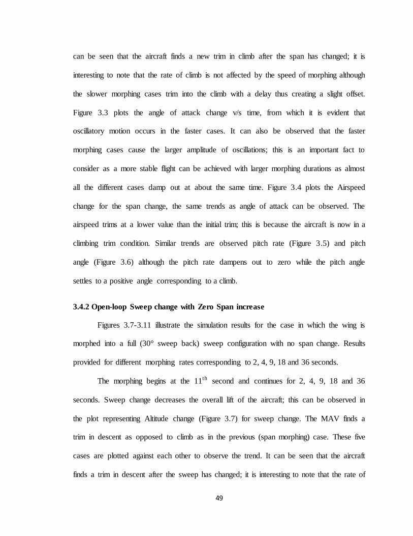
Figure 3.17 Altitude Change during controlled Span Morphing................................................ 57
x
Figure 3.18 Altitude Change during controlled Sweep Morphing ............................................. 57
Figure A.1 Wing Prototype ................................................................................................... 62
Figure A.2 Hitec-645MG Ultra Torque Servo ......................................................................... 65
Figure A.3 Speed/Direction Regulator.................................................................................... 65
Figure A.4 CCPM servo controller......................................................................................... 65
Figure A.5 Pressure Transducer/Condenser Microphone Locations .......................................... 67
Figure A.6 Results of Span Change at 0° AoA Plotted on XFOIL Pressure Distribution ............ 70
Figure A.7 Results of Span Change at 2° AoA Plotted on XFOIL Pressure Distribution ............ 71
Figure A.8 Results of Span Change at 4° AoA Plotted on XFOIL Pressure Distribution ............ 71
Figure A.9 Graphical Representation of Pressure Change for Sweep Change at 0° AoA ............ 73
Figure A.10 Graphical Representation of Pressure Change for Sweep Change at 2° AoA .......... 74
Figure A.11 Graphical Representation of Pressure Change for Sweep Change at 4° AoA .......... 74
Figure A.12 Snap Sweep at 4 Degrees AoA............................................................................ 77
Figure A.13 Section of Interest Filtered .................................................................................. 78
Figure A.14 PSD of the High-pass and Stop-band filter ........................................................... 78
Figure B.1 Calibration of Pressure Transducer Used at Station 4.............................................. 81
Figure B.2 Calibration of Pressure Transducer Used at Station 7.............................................. 81
Figure B.3 Calibration of Pressure Transducer Used at Station 10 ............................................ 82
Figure B.4 Electronics........................................................................................................... 82
Figure B.5 XFOIL CP at 0° AoA ........................................................................................... 84
Figure B.6 XFOIL Pressure Distribution at 0° AoA ................................................................ 85
Figure B.7 XFOIL CP at 2° AoA ........................................................................................... 85
Figure B.8 XFOIL Pressure Distribution at 2° AoA ................................................................ 86
Figure B.9 XFOIL CP at 4° AoA ........................................................................................... 86
Figure B.10 XFOIL Pressure Distribution at 4° AoA............................................................... 87

xi
List of Tables
Table 2.1 Surfaces Model Geometry ................................................................................ 13
Table 2.2 CL0 Values for various configurations............................................................. 17
Table 2.3 CL values for various configurations ............................................................. 18
Table 2.4 CLq values for various configurations.............................................................. 18
Table 2.5 CLe values for various configurations ............................................................ 18
Table 2.6 CD values for various configurations............................................................. 19
Table 2.7 Cm values for various configurations ............................................................ 19
Table 2.8 Cmq values for various configurations ............................................................. 20
Table 2.9 Cme values for various configurations ........................................................... 20
Table 2.10 Comparison between Classical calculations and SURFACES values……….22 Table 3.1 Eigenvalues of the Basic Configuration ........................................................... 41
Table 3.2 Eigenvalues of Full Sweep Configuration ........................................................ 41
Table 3.3 Eigenvalues of Full Span Configuration........................................................... 42
Table 3.4 Eigenvalues of Full Span Full Sweep Configuration........................................ 42
Table A.1 Change in Coefficient of Pressure from Pre to Post Span Morph ................... 69
Table A.2 Change in Coefficient of Pressure from Pre to Post Sweep Morph................. 72
Table B.1 Pressure Readings from Pre to Post Span Morph ............................................ 83
Table B.2 Coefficient of Pressure from Pre to Post Span Morph ..................................... 83
Table B.3 Pressure readings from Pre to Post Sweep Morph ........................................... 83
Table B.4 Coefficient of Pressure from Pre to Post Sweep Morph .................................. 84

1
CHAPTER 1: INTRODUCTION
Some of the earliest attempts at flight were aimed at emulating birds and focused
in particular on the construction of flapping wing mechanisms. Indeed, birds have
evolved into very efficient flying machines, and bio-inspired designs offer many potential
benefits for small UAVs. One of the most important and interesting aspects of avian
flight dynamics is how birds can change their shape to optimize flight in different
conditions. For the most part, these changes take place through morphing of the wings.
Wing morphing in birds can be viewed as an example to optimize aircraft performance
over a wider range of conditions. A morphing aircraft can be defined as an aircraft that
changes configuration in-flight to maximize its performance at significantly different
flight conditions. Since the propulsive power of MAVs is very limited, they stand to
benefit from being able to dramatically change their wing geometry in order to
accommodate wind gusts and other disturbances.
Figure 1.1 Side View of the wing bending in an MAV to achieve Roll control [1].
2
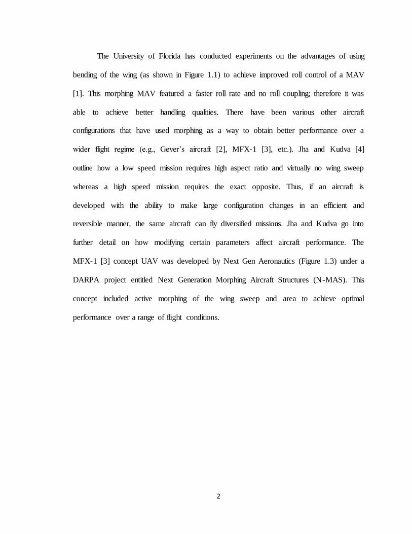
The University of Florida has conducted experiments on the advantages of using
bending of the wing (as shown in Figure 1.1) to achieve improved roll control of a MAV
[1]. This morphing MAV featured a faster roll rate and no roll coupling; therefore it was
able to achieve better handling qualities. There have been various other aircraft
configurations that have used morphing as a way to obtain better performance over a
wider flight regime (e.g., Gever’s aircraft [2], MFX-1 [3], etc.). Jha and Kudva [4]
outline how a low speed mission requires high aspect ratio and virtually no wing sweep
whereas a high speed mission requires the exact opposite. Thus, if an aircraft is
developed with the ability to make large configuration changes in an efficient and
reversible manner, the same aircraft can fly diversified missions. Jha and Kudva go into
further detail on how modifying certain parameters affect aircraft performance. The
MFX-1 [3] concept UAV was developed by Next Gen Aeronautics (Figure 1.3) under a
DARPA project entitled Next Generation Morphing Aircraft Structures (N-MAS). This
concept included active morphing of the wing sweep and area to achieve optimal
performance over a range of flight conditions.

3
Figure 1.2 Gevers Genesis 'tri-phibian' Aircraft [2].
Figure 1.3 MFX-1 Morphing Sweep-Span UAV [3].
Two of the most effective morphing parameters on an aircraft are wing sweep and
wing span. For span change, increasing aspect ratio increases lift-to-drag ratio, cruise
distance, turn rate, and decreases engine requirements. Decreasing aspect ratio increases
the maximum speed and decreases parasitic drag. One example of span change is the
telescoping wing on Gever’s aircraft (shown in Figure 1.2), and this is described in more
detail on the Gever’s aircraft website [2]. For sweep change, increasing sweep can
4
increase the critical Mach number, dihedral effect, and can decrease high speed drag
whereas decreasing sweep can increase the maximum lift coefficient. Examples of
variable-sweep aircraft include the Messerschmitt, P-1101, Bell X-5, XF101F-1 Jaguar,
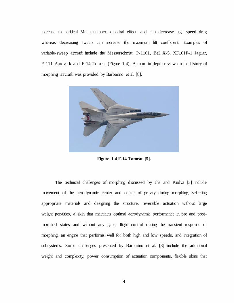
F-111 Aardvark and F-14 Tomcat (Figure 1.4). A more in-depth review on the history of
morphing aircraft was provided by Barbarino et al. [8].
Figure 1.4 F-14 Tomcat [5].
The technical challenges of morphing discussed by Jha and Kudva [3] include
movement of the aerodynamic center and center of gravity during morphing, selecting
appropriate materials and designing the structure, reversible actuation without large
weight penalties, a skin that maintains optimal aerodynamic performance in pre and post-
morphed states and without any gaps, flight control during the transient response of
morphing, an engine that performs well for both high and low speeds, and integration of
subsystems. Some challenges presented by Barbarino et al. [8] include the additional
weight and complexity, power consumption of actuation components, flexible skins that

5
remain tight in both pre and post-morphed states, and adequate flight control to handle
the changing aerodynamic and inertia characteristics of morphing vehicles.
Even though there has been considerable research done on the performance and
aerodynamics of morphing, there has not been much data or analysis on the transient
effects of morphing. Barbarino et al. [6], Jha and Kudva [4], and Weisshaar [7] all
mention the challenge of developing an adequate flight control to handle the changing
aerodynamic and inertia characteristics of morphing vehicles. A recent study was
conducted by Grant et al. [8] to analyze the modes of a variable-sweep MAV. The
frequency of change of the aerodynamics for this vehicle was of the same magnitude as
the rate of change of the wing sweep. Therefore, a linear time-varying (LTV) model was
required to properly analyze the morphing dynamics.
This thesis paper is structured as follows. A model of a variable sweep, variable
span morphing wing UAV is developed using the software SURFACES [9], which
employs the vortex lattice method (VLM) to model the aerodynamics. Using the
aerodynamic data resulting from this model, a nonlinear dynamic simulation of this
vehicle is then developed in order to simulate the dynamic response to changing the wing
span and sweep. Simulation results are presented and the dynamic effects and benefits of
morphing are then discussed.
1.1 MORPHING
Morphing can be defined as a transformation from one shape to another. There are
various examples around us where morphing can be observed in machines and in nature,
from enjoying sunshine in a convertible car on a sunny day to the closing of flower petals

6
to prevent pollen from becoming wet and heavy with dew so that insects can easily
transfer it [10].
A wing is designed as a compromise in geometry such that aircraft is able to fly at
a range of flight conditions, but the performance at each condition is often not optimized
or maximum possible efficiency is not obtained. The deployment of conventional flaps or
slats on a commercial airplane changes the geometry of its wings; these examples of
geometry changes are limited, with narrow benefits compared to those that could be
obtained from a wing that is inherently deformable and adaptable. The ability of a wing
surface to change its geometry during flight has interested researchers and designers over
the years. An adaptive wing diminishes the compromises required to insure operation of
the airplane in multiple flight conditions [11]. Aircraft like the F-14 Tomacat or Panavia
Tornado, which apply morphing technology to achieve better performance at both low
and high speeds, alleviating the problems of compressibility, are prime examples where
the performance benefits have outweighed the structural and weight penalties of
morphing. Recent developments in smart materials may overcome these penalties and
enhance the benefits of similar design solutions.
Figure 1.5 Classification of Wing Morphing [6].

7
Morphing in aircraft has been prevalent since the Wright Flyer, which used wing
twist to achieve roll control. New emerging technologies have rendered morphing both
more complex and efficient. Geometrical parameters that can be affected by morphing
solutions can be categorized into, as seen in Figure 1.5: planform alteration (span, sweep
and chord), out-of-plane transformation (twist, dihedral/gull and span-wise bending) and
airfoil adjustment (camber and thickness) [6].
1.1.1 Wing Planform Morphing
Wing planform morphing affects three parameters; span, chord and sweep. Span and
sweep affect the wing aspect ratio which modifies the lift to drag ratio of the vehicle. An
increase in wing aspect ratio would thus result in an increase in range and endurance.
Aerodynamically, change in aspect ratio produces a change in the lift curve slope and
forces due to the change in area. Dynamically, the inertias of the aircraft also change.
Chord extensions have been adopted in rotary flights as it is easier (mechanically) to
change the chord of a rotor than it is to attempt change of chord on a fixed wing given the
structural constrains and the position of fuel tanks in the wings. A study on quasi-
statically increasing the chord through the extension of a flat plate on a rotor appeared to
give better high lift performances than trailing edge or Gurney flaps [12].
1.1.2 Wing Out-of-Plane Transformation
This is mainly affected by three parameters (individually or in combination): twist
dihedral/gull and span-wise bending. Wing aeroelastic twist can be used to produce the
required roll moments for control; this can allow the aircraft to operate beyond the

8
dynamics pressure limits where aileron reversal would conventionally begin. The
Variable Stiffness Spar (VSS) was developed to vary the torsional stiffness of wings to
enhance the roll performance of an aircraft (depicted in Figure 1.6). The concept allows
the stiffness and aeroelastic behavior of the wing to be controlled as a function of flight
conditions [13]. The VSS concept was further advanced to develop a torsion free wing
that allowed for significant aeroelastic amplification to increase the roll rate by 8.44% to
48% above baseline performance. [14]. A wing morphing mechanism was developed in
2005 to vary wing twist to control a swept wing tailless aircraft. Initial wind tunnel tests
showed that this mechanism was able to provide adequate forces and moments to control
a UAV and potentially a manned aircraft. It also adds the benefit of allowing the aircraft
to fly in cruise without the added drag of washout or winglets used to counter the adverse
yaw. Tests showed a promising improvement of 15% in the lift to drag ratio when
compared to an elevon-equipped wing with built-in 10° washout [15]. A variable
dihedral/gull wing has the ability to control the aerodynamic span; replace conventional
control surfaces, enhance the agility and flight characteristics of high performance
aircraft, reduce induced drag by changing the vorticity distribution and improve stall
characteristics [6]. Although out-of-plane morphing is the least common type of
morphing solution, recently there has been considerable interest in this method because
of the significant impact on the aerodynamic behavior of a control surface without large
planform modifications.

9
Figure 1.6 Photo of wing surface showing a steel VSS [16].
1.1.3 Airfoil Morphing
Airfoil morphing is the most dominant research topic in morphing methods with more
focus being given to camber morphing concepts. The most common method of airfoil
morphing is by conventional actuator methods, although with the advent of composites
and smart materials, the use of SMA (Shape Memory Alloys), PZT (Piezoelectric
materials) and RMA (Rubber Muscle Actuators) has also been studied. The first camber
morphing examples stem from the early 1920’s where the wing configuration was
changed through the aerodynamic loads on the wing. Wind tunnel tests showed that the
wing had a maximum lift coefficient of 0.76 and a minimum drag of 0.007 [17]. Research
has also shown that optimal control of the camber can provide an efficient means of
improving the L/D ratio at each flight condition during the unsteady phases of periodic
optimal endurance cruise and fuel consumption is also minimized during the idle phase
[18]. MAV’s fly at low Reynolds numbers typically in the range of 10,000-100,000; in
this region, flow separation on the airfoil can lead to a sudden increase in drag and loss of
efficiency. Thus aerodynamic efficiency is critical for MAV design. Active camber

10
control can overcome some of the problems of MAV design like flow separation due to
low Reynolds number that reduces effectiveness of a trailing edge control surface,
elimination/reduction of control surface drag as MAV’s/UAV’s have severe power
constraints and an active control surface has the opportunity to provide flow control due
to its direct effect on circulation. Example of an Adaptive-Twist airfoil is shown in
Figure 1.7, this model was used to analyze and study active camber changes and their
effects on aircraft [19].
Figure 1.7 Tip of Experimental Adaptive-Twist airfoil [19].
Overall it can be argued that, after over a century of flight the aircraft industry has
reached a point where the industry can now consider the pursuit of more efficient aircraft
configurations that are not optimized to a limited flight regime and purpose. Millions of
years of natural evolution have made birds the most efficient flying machines on the
planet. Their versatility and ability to adapt to different flight environments and
adversities such as wind gusts is unparalleled. Birds have also developed an ability to
harvest lift out of nature through thermals and wind shears. Micro Air Vehicles in general
lack the propulsive ability to ascend to higher altitudes for loitering and surveillance, and
it would be potentially beneficial to program MAVs to utilize thermals and other wind
patterns to achieve lift to enhance the endurance of the vehicle. To conceptualize such a
system would require a wider range of performance that would be impossible for a MAV
if not for morphing. Wing morphing to change the wing geometry would provide a bio-
11
inspired scenario for utilization of nature to achieve more efficient lift. With the advent of
smart materials the industry is now at a stage where a more intensive study of morphing
can be performed without all the weight penalties associated with mechanically morphing
the wing and their feasibility can be determined.
1.2 TECHNICAL OBJECTIVES
The design of a morphing wing UAV is developed using the wing test model as a
reference. This design is then modeled in SURFACES software [9], which employs the
vortex lattice method (VLM) to model the aerodynamics. Using the aerodynamic data
resulting from this model, a nonlinear dynamic simulation of this vehicle is then
developed in order to simulate the dynamic response to changing the wing span and
sweep. Simulation results are presented and the dynamic effects and benefits of morphing
are discussed.
In context of this thesis the author will study some changes which take place
during morphing and some affects the speed of morphing plays in the dynamics. This will
outline the benefits of morphing and provide insight into the dynamic effects of
morphing.
12
CHAPTER 2: SURFACES MODEL
Classically any airplane preliminary static/dynamic analysis was carried out by
either wind tunnel experiments, which are expensive and time consuming, or by the use
of statistical estimation methods, which are tedious. With the advent of vortex lattice
solvers, aircraft designers have obtained a relatively simple tool that gives them a basic
idea of the dynamics of the aircraft without going through the cumbersome process of
building a prototype for wind tunnel testing.
The VLM solver used for this research project is called ‘SURFACES’, which is
developed and distributed by Flight Level Engineering. SURFACES uses a three-
dimensional Vortex Lattice Method (VLM) to determine airflow around the aircraft,
allowing the user to extract a large amount of information from the solution ranging from
elementary plotting of the flow solution to sophisticated extraction of loads and stability
derivatives [9].
A preliminary model is constructed in SURFACES and the geometries and
weights are set up. Panels are then defined onto the geometry; these panels have a control
volume over which flow is analyzed. The program uses built-in inertia modeling to
determine the moments and products of inertias; it also uses the geometry and the defined
weight distributions for statistical analysis to determine the neutral point and CG
location. Control surfaces and high lift devices such as elevator, rudder, ailerons, flaps,
and slats etc. can be incorporated and used to trim the aircraft about the three axes at a

13
desirable speed, altitude, CG and power setting. SURFACES uses math objects to
determine performance and stability derivatives and automatically computer properties
by using model geometry directly, Vortex-Lattice results and others. Force Integrators are
used to determine shear and moments about 3-axes on any surface in any orientation and
the program can account for thrust, symmetric or asymmetric. [9]
2.1 MODELING
The model created in SURFACES was based on a morphing wing design used for
the wind tunnel experiments; a conventional T-Tail configuration was chosen for the
design purpose. A preliminary model was created with the set of dimensions given in
Table 2.1.
Table 2.1 Surfaces Model Geometry.
Wing Horizontal Tail Vertical Tail Fuselage
S = 3.5ft2 Bht = 1.5ft Bvt = 0.75ft. L = 4.25 ft.
C = 1 ft. Sht = 0.75 ft2 Svt = 0.25ft2
This configuration was designated as the 0 Span 0 Sweep base model (Figure 2.1) and
then the wings were swept back by an angle of 5 degrees for each configuration while the
span was increased by 10% (0.03’) for each configuration, creating a total of 77 different
models that conform to the full range of sweep/span configuration that can be achieved
by the MAV.

14
Figure 2.1 SURFACES Model for 10% Span Increase.
Figure 2.2 SURFACES Model for 50% Span, 30 degree Sweep.
Movement of CG and Neutral Point
Retention of wing tip after sweep
CG
Neutral Point
Moving Servo motor to maintain static margin

15
One of the most important aspects to consider while designing a morphing aircraft
is the neutral point shift that takes place during sweep change. This in turn creates a
change in static margin, making it larger as the wings sweep back to a larger angle. This
phenomenon would make the aircraft more stable and less maneuverable, hence defeating
the purpose of morphing. To counteract this change, a novel mechanism was designed
that includes a slider rail in which the servo motors and batteries move in the direction of
the sweep (back). This causes the CG to shift back with the Neutral Point making the
static margin change less prominent. There is no mechanical way of negating the static
margin change apart from compartmentalizing the wing and changing the sweep on the
outboard section only, but this would make the mechanism more complicated. Using this
mechanism the static margin for all configurations was limited to under or around 15%.
Another matter of concern in this design is the retention of the outboard wing
shape after sweeping the wing back (Figure 2.1, 2.2); in a conventional morphing wing
the wing tips would no longer be parallel to the oncoming wind and therefore the
outboard wing design would have to be modified to incorporate the change. The author
realizes the affects that wing tip vortices may cause to the aircraft dynamics but suggests
(even if only theoretically) a design akin to one of a wind shield wiper commonly used in
cars with hinged ends to avoid the twisting of the wing tips. This would marginally
reduce changes in the tip vortices while simplifying the modeling complexity.
The design and evaluation techniques for large aspect ratio and high Reynolds
number fixed wing aircraft are well developed; however vortex lift problems on low
Reynolds number MAVs have made it difficult to extend the same codes. Very little
information is available on the performance of existing airfoil/wing shapes at low speeds
16
due to this issue. Therefore, extensive wind tunnel testing of the models is necessary to
validate any results obtained from computational methods. As the purpose of this thesis is
carrying out preliminary analysis and based on the fact that SURFACES provides a very
good estimation of the dynamics of the aircraft, the data obtained from the VLM solver
are used for the simulation studies presented in this thesis.
2.2 SIMULATION
This thesis work assumes that the stability derivatives change with morphing is a
quasi-steady change; this assumption could be verified fairly simply if it can be proven
that the frequency of change of the circulation on a wing is much greater than the
frequency of the morphing change.
L=ρ∞V∞ Γ b
Where, L = lift generated by the wing
ρ∞ = density of free-stream
V∞ = free-stream velocity
Γ = Circulation
b = span of the wing
The dimensions of Γ are m2/s; hence, if the circulation is multiplied by the cross-sectional
area of the wing; frequency of the change can be obtained. Substituting values obtained
from the geometry and aerodynamic data from classical calculations we obtain the
frequency of circulation to be around 12 hertz, whereas the frequency of change for the

17
fastest rate of morphing is an order of magnitude lower than that. Therefore it is safe to
assume this to be a quasi-steady system and proceed with the results obtained from
SURFACES.
The models representing the different morphing configurations were estimated
according to the Vortex-Lattice Method. SURFACES provide the Aerodynamic center,
CG and the Moment of Inertias calculated on the basis of the geometry of the aircraft
model. These values are further used to find the trim conditions, which in turn leads to
the calculation of the stability derivatives for the aircraft using classical methods. The
results obtained are then classified according to the configurations and different
derivatives are graphed with respect to sweep and span in order to identify trends. For the
purposes of this study, changes in the longitudinal stability derivatives are considered.
The stability derivatives obtained from SURFACES for all the given configurations are
listed below; here the rows indicate different span configurations whereas the columns
signify the sweep angles.
Table 2.2 CL0 values for various configurations.
0 10 20 30 40 50 60 70 80 90 100
0 0.161 0.165 0.168 0.170 0.173 0.183 0.188 0.188 0.197 0.202 0.205
5 0.156 0.159 0.160 0.160 0.162 0.164 0.164 0.165 0.167 0.168 0.169
10 0.153 0.155 0.156 0.157 0.158 0.159 0.161 0.162 0.163 0.164 0.165
15 0.148 0.150 0.152 0.152 0.154 0.155 0.155 0.157 0.158 0.159 0.160
20 0.142 0.143 0.144 0.145 0.147 0.148 0.149 0.149 0.151 0.152 0.153
25 0.135 0.136 0.137 0.139 0.140 0.141 0.143 0.143 0.145 0.144 0.147
30 0.126 0.128 0.129 0.130 0.132 0.132 0.134 0.134 0.136 0.137 0.138
CL0 is the coefficient of lift at zero angle of attack, on a CL v/s graphs the slope of the
line is represented by CLwhereas the y-axis intercept is known as CLo.

18
Table 2.3 CL values for various configurations.
0 10 20 30 40 50 60 70 80 90 100
0 3.962 4.008 4.068 4.109 4.161 4.211 4.313 4.313 4.524 4.628 4.650
5 3.699 3.730 3.755 3.782 3.807 3.833 3.857 3.882 3.908 3.932 3.956
10 3.679 3.710 3.734 3.762 3.786 3.813 3.837 3.862 3.887 3.911 3.935
15 3.638 3.669 3.693 3.720 3.745 3.773 3.795 3.820 3.845 3.870 3.893
20 3.578 3.609 3.632 3.660 3.685 3.704 3.734 3.758 3.782 3.806 3.830
25 3.494 3.526 3.549 3.576 3.596 3.627 3.651 3.675 3.739 3.699 3.757
30 3.386 3.418 3.443 3.471 3.497 3.523 3.547 3.571 3.595 3.618 3.641
Table 2.4 CLq values for various configurations.
0 10 20 30 40 50 60 70 80 90 100
0 7.729 7.822 7.960 7.904 8.048 8.258 8.262 8.262 8.491 8.478 8.268
5 7.752 7.681 7.661 7.614 7.549 7.475 7.439 7.473 7.380 7.380 7.506
10 7.921 7.879 7.810 7.735 7.700 7.730 7.694 7.672 7.614 7.625 7.689
15 8.055 8.021 7.921 7.886 7.823 7.782 7.834 7.782 7.724 7.730 7.826
20 8.217 8.100 7.990 7.979 7.934 7.929 7.875 7.845 7.782 7.749 7.872
25 8.407 8.182 8.148 8.078 8.055 8.014 7.983 7.966 7.929 7.876 7.952
30 8.792 8.623 8.548 8.582 8.416 8.357 8.299 8.258 8.113 8.113 8.190
Table 2.5 CLe values for various configurations.
0 10 20 30 40 50 60 70 80 90 100
0 0.545 0.536 0.526 0.517 0.508 0.547 0.548 0.548 0.548 0.549 0.461
5 0.547 0.537 0.530 0.522 0.514 0.506 0.499 0.491 0.485 0.478 0.471
10 0.552 0.542 0.534 0.526 0.518 0.511 0.503 0.496 0.489 0.482 0.475
15 0.559 0.549 0.541 0.533 0.525 0.518 0.510 0.503 0.496 0.489 0.482
20 0.569 0.559 0.551 0.543 0.535 0.452 0.520 0.513 0.505 0.498 0.492
25 0.578 0.568 0.560 0.551 0.463 0.536 0.528 0.521 0.507 0.514 0.501
30 0.524 0.513 0.506 0.497 0.489 0.484 0.477 0.474 0.467 0.462 0.459
CLq indicates the change in lift with respect to the pitch rate of the aircraft; in terms of
aircraft dynamics it represents a pitch damping coefficient. CLe is the change in lift due

19
to the elevator deflection; it represents the control effort of the elevator on the aircraft.
CDcan be represented as the change in drag with respect to the angle of attack of an
aircraft.
Table 2.6 CD values for various configurations.
0 10 20 30 40 50 60 70 80 90 100
0 0.195 0.189 0.184 0.179 0.210 0.218 0.227 0.228 0.238 0.245 0.247
5 0.196 0.190 0.186 0.178 0.177 0.172 0.166 0.161 0.160 0.156 0.152
10 0.200 0.193 0.188 0.182 0.179 0.175 0.170 0.166 0.162 0.159 0.155
15 0.203 0.197 0.193 0.187 0.180 0.178 0.171 0.170 0.166 0.162 0.158
20 0.210 0.203 0.199 0.191 0.187 0.183 0.178 0.173 0.171 0.167 0.163
25 0.217 0.211 0.206 0.200 0.194 0.191 0.185 0.182 0.180 0.175 0.170
30 0.225 0.219 0.212 0.208 0.203 0.196 0.194 0.191 0.187 0.182 0.178
Table 2.7 Cm values for various configurations.
0 10 20 30 40 50 60 70 80 90 100
0 -0.32 -0.32 -0.32 -0.31 -0.32 -0.31 -0.31 -0.31 -0.32 -0.32 -0.31
5 -0.31 -0.31 -0.31 -0.31 -0.31 -0.31 -0.31 -0.31 -0.31 -0.31 -0.31
10 -0.38 -0.44 -0.38 -0.39 -0.39 -0.42 -0.43 -0.43 -0.43 -0.45 -0.45
15 -0.44 -0.48 -0.43 -0.44 -0.45 -0.46 -0.47 -0.49 -0.50 -0.51 -0.52
20 -0.49 -0.52 -0.46 -0.47 -0.48 -0.50 -0.51 -0.53 -0.51 -0.53 -0.53
25 -0.52 -0.54 -0.49 -0.51 -0.50 -0.50 -0.52 -0.54 -0.55 -0.55 -0.55
30 -0.53 -0.54 -0.54 -0.55 -0.55 -0.55 -0.56 -0.57 -0.57 -0.56 -0.58
Cm is defined as the change in pitching moment with respect to the angle of attack, for a
stable aircraft this aero coefficient is negative. Cmq, also known as pitch damping, is the
change in pitch moment with respect to the pitch rate. This is mainly a damping effect
from the tail. As the aircraft pitched up, for example, the tail rotates downward relative to
the CG. This increases the angle of attack of the horizontal tail, which generates a lift
increment, which in turn generates a downwards pitching moment opposing the direction
of the pitch rate. Cme is the change in the pitching moment due to elevator control effort;

20
this is the change in lift due to elevator deflection CLe multiplied by the moment arm
between the center of gravity of the aircraft and the horizontal tail.
Table 2.8 Cmq values for various configurations.
0 10 20 30 40 50 60 70 80 90 100
0 -15.0 -15.0 -15.0 -15.0 -15.0 -15.0 -15.0 -15.0 -15.0 -15.0 -14.9
5 -14.7 -14.5 -14.2 -14.0 -13.8 -13.6 -13.4 -13.2 -13.0 -12.9 -12.7
10 -14.7 -14.6 -14.2 -14.1 -13.9 -13.7 -13.5 -13.3 -13.1 -13.0 -12.9
15 -14.9 -14.7 -14.4 -14.2 -14.0 -13.8 -13.6 -13.5 -13.3 -13.1 -13.0
20 -15.2 -14.9 -14.6 -14.4 -14.2 -14.0 -13.8 -13.7 -13.4 -13.3 -13.1
25 -15.6 -15.3 -15.0 -14.8 -14.5 -14.4 -14.2 -14.1 -13.9 -13.8 -13.5
30 -17.0 -16.6 -16.3 -16.1 -15.8 -15.5 -15.3 -15.0 -14.8 -14.5 -14.3
Table 2.9 Cme values for various configurations.
0 10 20 30 40 50 60 70 80 90 100
0 -1.81 -1.77 -1.81 -1.80 -1.80 -1.80 -1.80 -1.80 -1.80 -1.80 -1.80
5 -1.78 -1.75 -1.72 -1.69 -1.66 -1.64 -1.61 -1.59 -1.57 -1.54 -1.52
10 -1.78 -1.75 -1.72 -1.69 -1.66 -1.64 -1.62 -1.59 -1.57 -1.55 -1.51
15 -1.78 -1.75 -1.72 -1.69 -1.67 -1.64 -1.62 -1.59 -1.57 -1.55 -1.52
20 -1.80 -1.77 -1.73 -1.71 -1.68 -1.65 -1.63 -1.60 -1.58 -1.55 -1.53
25 -1.81 -1.77 -1.74 -1.72 -1.69 -1.66 -1.63 -1.61 -1.56 -1.54 -1.53
30 -1.63 -1.59 -1.56 -1.53 -1.50 -1.48 -1.45 -1.44 -1.42 -1.40 -1.38
These values were then verified by classical hand calculations based on the formulas of
longitudinal dynamic stability which calculate the aerodynamic coefficients based on the
geometrical parameters of the design and aerodynamic properties obtained from the
airfoil section [20]. The formulas and the results are mentioned below [21]:
CLq=2ηCLαtVH
CLδe= St
Sw
ηdCLt
dδe=
St
Sw
ηCLαtτ
21
Cmα= CLαw (XCG
c-
Xac
c) -ηCLαtVH (1-
dε
dα) ,
dε
dα =
2CLαw
πAR
Cmq= -2ηCLαtVH
lt
c
Cmδe=-ηVH
dCLt
dδe = -ηVHCLαtτ
Here, Clα = lift curve slope of the infinite wing span
η = tail efficiency factor = 0.9
CLαt = lift curve slope of the horizontal tail
VH = tail volume = 0.6696
St = tail area = 0.75ft2
SW = wing area = 3.5ft2
τ = flap effectiveness factor [21] = 0.4
XCG = x-location of the CG
Xac = x-location of the aerodynamic center
AR = aspect ratio = 3.5
lt = distance between CG of tail to the CG of the aircraft = 2.75ft
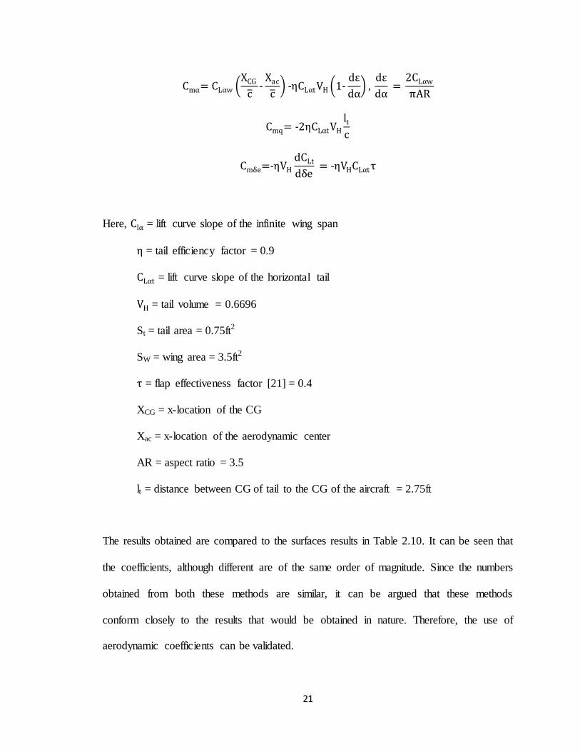
The results obtained are compared to the surfaces results in Table 2.10. It can be seen that
the coefficients, although different are of the same order of magnitude. Since the numbers
obtained from both these methods are similar, it can be argued that these methods
conform closely to the results that would be obtained in nature. Therefore, the use of
aerodynamic coefficients can be validated.
22
Table 2.10 Comparison between Classical calculations and SURFACES values .
SURFACES
Classical Calculations
CL 3.96 4.01
CLq 7.73 4.32
CLe 0.55 0.28
Cm -0.32 -0.52
Cmq -15 -11.88
Cme -1.81 -0.86
2.3 ANALYSIS
It can be noted that, with sweep and span variation, various patterns of change are
observed in the longitudinal stability derivatives. Some of the results are mentioned
below with plausible explanations for these effects. It should be noted here that all the
analysis is based on changes in a longitudinal model.
2.3.1 CL coefficients
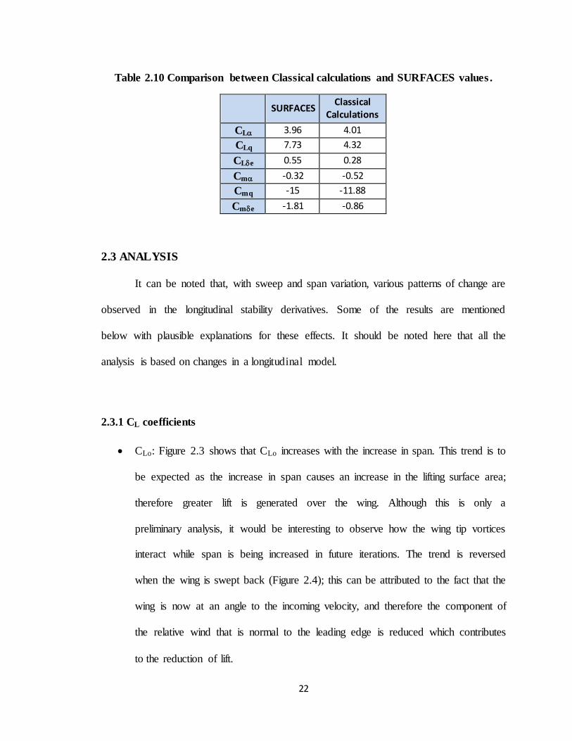
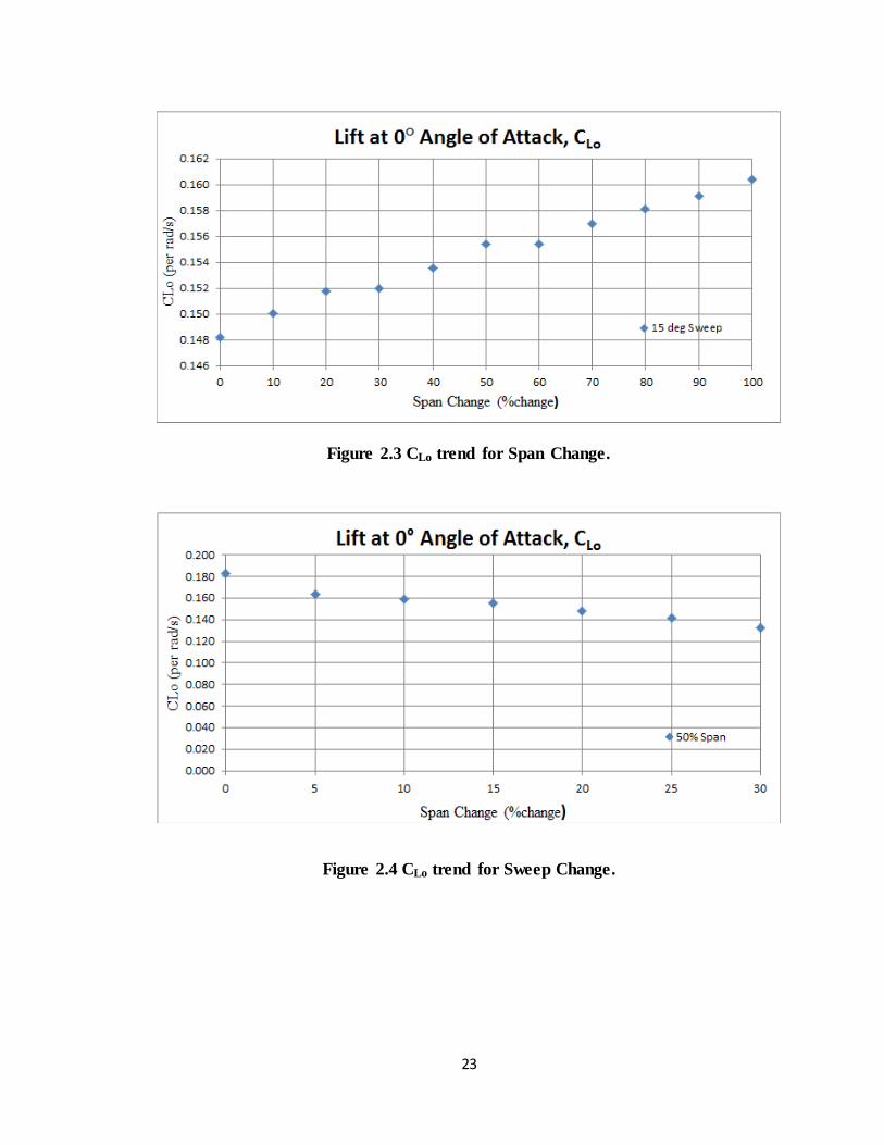
CLo: Figure 2.3 shows that CLo increases with the increase in span. This trend is to
be expected as the increase in span causes an increase in the lifting surface area;
therefore greater lift is generated over the wing. Although this is only a
preliminary analysis, it would be interesting to observe how the wing tip vortices
interact while span is being increased in future iterations. The trend is reversed
when the wing is swept back (Figure 2.4); this can be attributed to the fact that the
wing is now at an angle to the incoming velocity, and therefore the component of
the relative wind that is normal to the leading edge is reduced which contributes
to the reduction of lift.
23
Figure 2.3 CLo trend for Span Change.
Figure 2.4 CLo trend for Sweep Change.

24
Figure 2.5 CL trend for Span Change.
Figure 2.6 CL trend for Sweep Change.
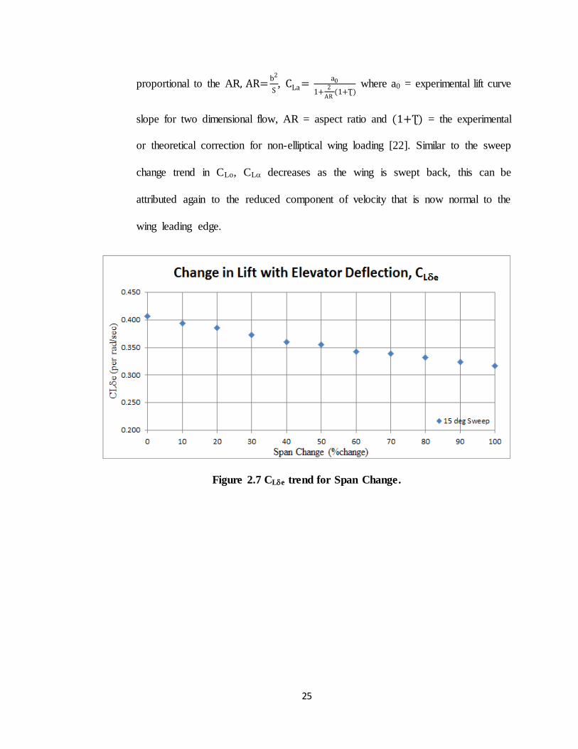
CL: Figure 2.5 and 2.6 show a similar trend as the observed span and sweep
change in CLo. The lift curve slope increases as the span increases because the
aspect ratio is lowered as the wing becomes more slender. CL is inversely
25
proportional to the AR, AR=b2
S, CLa =
a0
1+2
AR (1+Ʈ)
where a0 = experimental lift curve
slope for two dimensional flow, AR = aspect ratio and (1+Ʈ) = the experimental
or theoretical correction for non-elliptical wing loading [22]. Similar to the sweep
change trend in CLo, CL decreases as the wing is swept back, this can be
attributed again to the reduced component of velocity that is now normal to the
wing leading edge.
Figure 2.7 CLe trend for Span Change.
26
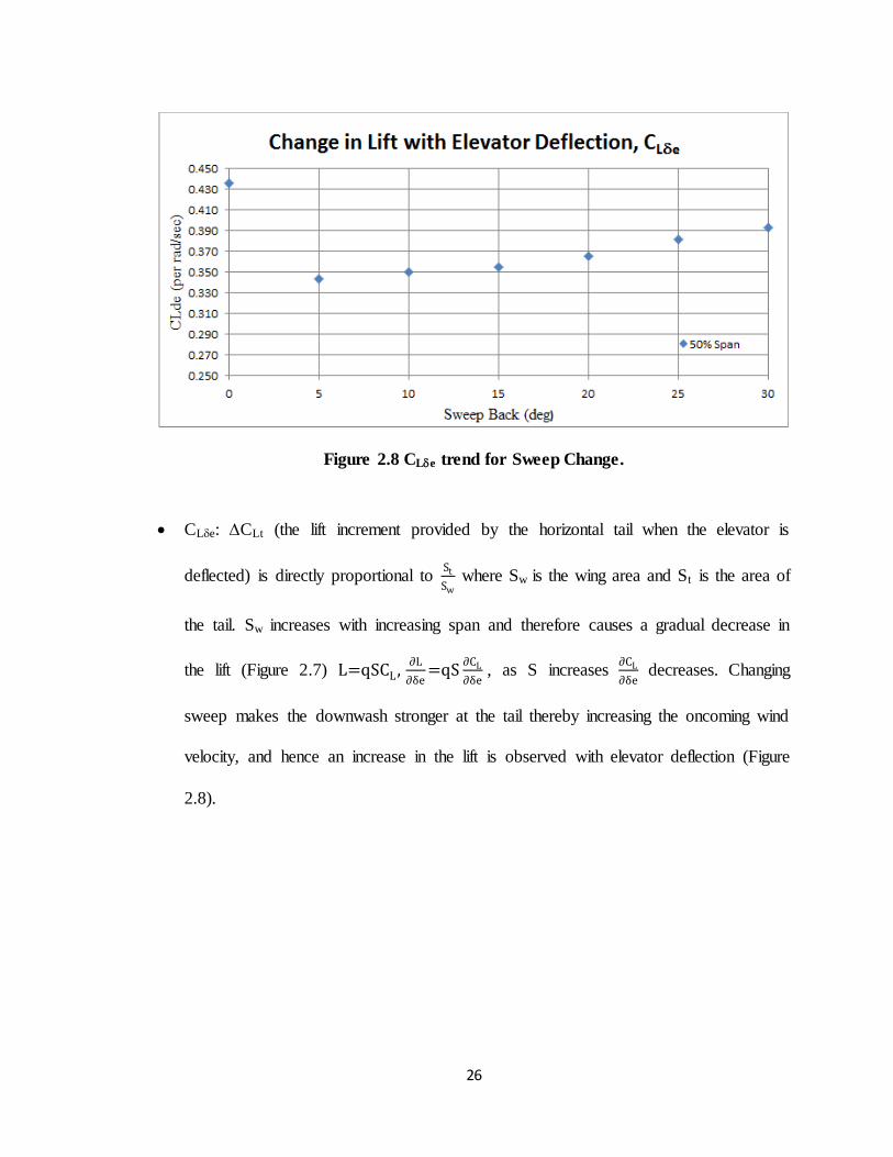
Figure 2.8 CLe trend for Sweep Change.
CLe: CLt (the lift increment provided by the horizontal tail when the elevator is
deflected) is directly proportional to St
Sw where Sw is the wing area and St is the area of
the tail. Sw increases with increasing span and therefore causes a gradual decrease in
the lift (Figure 2.7) L=qSCL , ∂L
∂δe=qS
∂CL
∂δe , as S increases
∂CL
∂δe decreases. Changing
sweep makes the downwash stronger at the tail thereby increasing the oncoming wind
velocity, and hence an increase in the lift is observed with elevator deflection (Figure
2.8).

27
Figure 2.9 CLq trend for Span Change.
Figure 2.10 CLq trend for Sweep Change.
CLq: is the change in lift coefficient in response to pitch rate which is mainly a
horizontal tail effect. When the aircraft has a positive (nose up) pitch rate, the
horizontal tail rotates downward relative to the CG this increases the angle of

28
attack of the horizontal tail, which increases the lift. As the wing span increases,
this coefficient decreases in large part because the increment in the aircraft lift
coefficient due to tail lift is proportional to St
Sw, the ratio of tail to wing surface
area, which decreases as wing span increases. When sweep increases, CLq is seen
to increase (Figure 2.9) which is likely caused by the increase in lift at the tail due
to the increased downwash angle at the horizontal tail due to the close proximity
of the wing tips to the tail for the swept back configuration (Figure 2.10).
2.3.2 CD coefficients
Figure 2.11 CD trend for Span Change.

29
Figure 2.12 CD trend for Sweep Change.
CD: There is a slight decrease in the drag when the span is increased (Figure
2.11), this trend is caused by the decrease in induced drag of the aircraft as the
aspect ratio is increased. An aircraft with infinite aspect ratio would theoretically
produce zero induced drag. Sweeping the wings back, on the contrary, provides
more area for wing tip vortices to form along the span of the wing, thus creating a
higher induced drag. This can be observed in Figure 2.12.

30
2.3.3 Cm coefficients
Figure 2.13 Cm trend for Span Change.
Figure 2.14 Cm trend for Sweep Change.

31
Cm: Span change has very little effect on Cmas shown in Figure 2.13 but due
to the movement of the center of gravity of the aircraft while sweeping the wings
back there is an increase in the moment arm from the aerodynamic wing to the
CG, which generates a higher Cm as seen in Figure 2.14.
Figure 2.15 Cme trend for Span Change.
Figure 2.16 Cme trend for Sweep Change.
32
Cme: There is a slight decrease in the pitch moment coefficient due to elevator
defection (Figure 2.15) while changing the span; this trend is in direct correlation
with CLe as Cme is the change in lift caused by elevator deflection multiplied by
the moment arm between the CG of the aircraft and the horizontal tail. Sweep
change (Figure 2.16), however, decreases Cme which can be described by the
change in the CG of the aircraft similar to the trend observed in Figure 2.8.
Figure 2.17 Cmq trend for Span Change.

33
Figure 2.18 Cmq trend for Sweep Change.
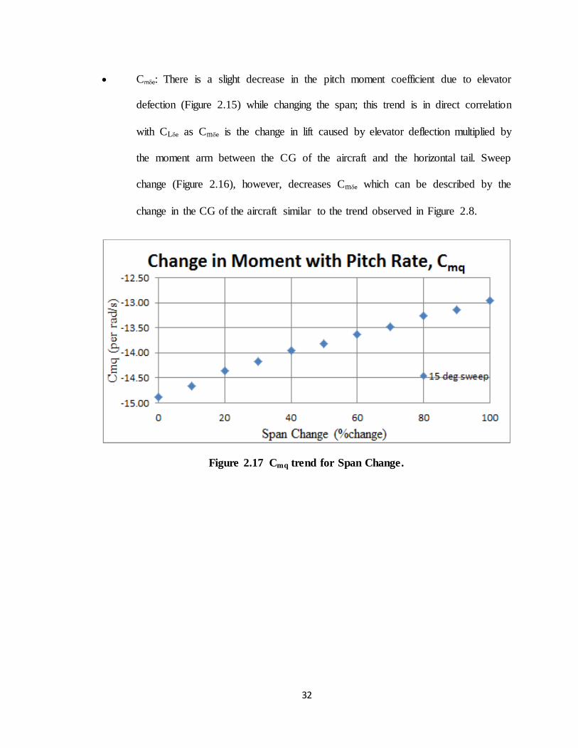
Cmq: As can be observed in Figure 2.17, there is a steady decrease in the
magnitude of pitch damping due to change in span, which can be attributed to the
same trend as observed in CLq, since change in lift at the horizontal tail causes
change in the pitch moment about the center of gravity. The evident increase in
pitch damping while sweeping the wing back is due to the movement of the CG
and the aerodynamic center (static margin) further away from each other; this
causes the moment arm to increase, thereby increasing the magnitude of pitch
damping as the wing is swept back.
34
CHAPTER 3: SIMULATION DEVELOPMENT AND CONTROL
DESIGN
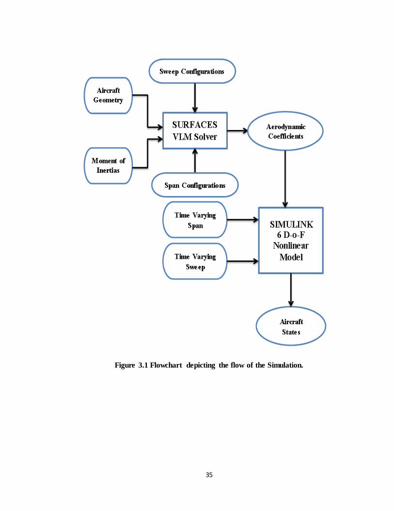
The aerodynamic coefficients obtained from SURFACES of the 77 different
configurations for every combination of sweep back and span changes were used to
construct a look up table for the longitudinal coefficients. These tables were then used to
simulate the changing dynamics of the aircraft during morphing. 6 degrees of freedom
model was then built to simulate the non-linear dynamic equations of an aircraft. This
SIMULINK model was then modified to incorporate a linear trajectory of sweep and
span morphing at desired rates. Data obtained from SURFACES for various
configurations of the aircraft was interpolated to form data tables, these tables serve as a
reference to the non-linear model. For every time step during change in sweep and/or
span of the aircraft longitudinal aerodynamic coefficients referenced for those particular
configurations are fed into the model in real time. This created a real time dynamic
simulation used to study the change in the longitudinal modes of the UAV. A state
feedback controller was then designed as a stability augmentation system to enable the
aircraft to maintain altitude throughout the flight. This flow of the simulation can be
observed in Figure 3.1.
35
Figure 3.1 Flowchart depicting the flow of the Simulation.

36
3.1 NON-LINEAR SIMULINK MODEL
A 6-degrees-of-freedom nonlinear aircraft Simulink model with modifications set
up to simulate wing morphing was developed to study the dynamic response of the
morphing aircraft. The aircraft dynamic model includes the nonlinear rigid body
equations of motion which take the form; x(t)=f (x(t), u(t), t) where the state vector is
defined as x(t)= u, v, w, p, q, r, ∅, θ, φ, XN, YE, ZDT and the control vector is defined as
u(t) = 𝛿𝑒 ,𝛿𝑇 ,𝛿𝑎 , 𝛿𝑟. The nonlinear equations of model are represented by f which time
is varying due to morphing. The longitudinal aerodynamic forces and moments are
dependent on the wing morphing configuration. Aerodynamic data from obtained from
SURFACES is used to generate 2-D tables of aerodynamic coefficients as a function of
sweep and span. The simulation then interpolates the aerodynamic data from these tables
to compute the appropriate aero-coefficients for the current span and sweep of the
vehicle. The model was configured to inculcate time variant change in the sweep and
span morphing so that geometry could be varied in different time intervals, this would
help us better understand the transient effects speed of morphing has on the dynamics of
an MAV. A chart depicting the simulation process is provided in Figure 3.1.
Time varying morphing functions was incorporated into the Simulink model in
order to independently vary the wing span and sweep in the simulation. For the studies
performed in this thesis the sweep and span were varied as a linear function of time:
b=bo+(bf-bo)
T∙t
=o+(f-o)
T∙t

37
Where, b, = current span/sweep
bo ,o = initial span/sweep
𝑏𝑓 ,𝑓 = final span/sweep
T = time taken to reach from initial to final morphing geometry
t = current time step
Note that these functions are designed so that the morphing rate can be varied as a
parameter in the simulation. These morphing functions can be easily modified to model
different morphing trajectories, such as quadratic morphing function. At each step, the
span and sweep are input to the aerodynamic tables that were generated using
SURFACES data, as can be observed in Figure 3.1
3.2 DYNAMIC MODE ANALYSIS
Trim conditions for the aircraft are determined in order to make the aircraft fly
straight and level, those values are further used to linearize the model at the trim. This
process corresponds to finding the angle of attack, elevator deflection and thrust for
which the aircraft attains a longitudinal equilibrium (i.e. longitudinal forces and moments
sum to zero). The 3 longitudinal equilibrium conditions to be satisfied for level flight are
as follows:
T0+CLtrimQS sin(α) -CDtrim
QS cos(α) -Wsin (α) = 0
-CLtrimQS cos(α) -CDtrim
QS sin(α) +Wcos(α) = 0
CmtrimQSc = 0

38
Where, CLtrim=CLo
+CLαα+CLδe
δe
CDtrim=CDo
+CDαα+CDδe
δe
Cmtrim= Cmo
+Cmαα+Cmδe
δe
Q = dynamic pressure
S = wing area
c = wing chord
And α, δe and T0 are the angle of attack, elevator deflection and thrust
respectively, these three equations are solved to obtain the three trim variables.
In order to study the dynamic stability of the morphing aircraft, the nonlinear
dynamic model was linearized about the trim state corresponding to each of the 4
morphing configurations shown in Table 3.1-3.4. This process generated a family of
linearized longitudinal models of the form:
∆X(t)=[A]∆X(t)+[B]∆U(t)
Where,
∆X =∆u, ∆w, ∆q, ∆θT
∆U = ∆δe, ∆δT
Note that the linearized state and control vectors (∆X, ∆U ) correspond to the
change in the state and control vector from the equilibrium values ∆𝑋𝑜,∆𝑈𝑜. Only 4
longitudinal states were included in the linear model because the other 2 longitudinal
39
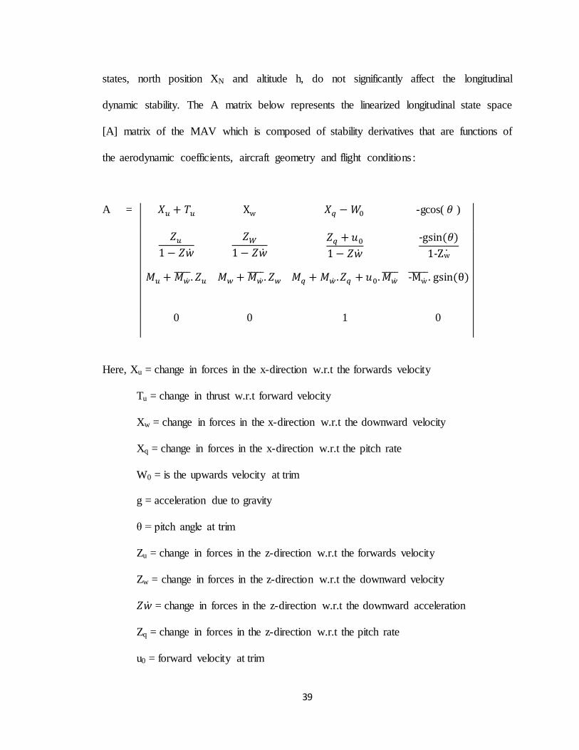
states, north position XN and altitude h, do not significantly affect the longitudinal
dynamic stability. The A matrix below represents the linearized longitudinal state space
[A] matrix of the MAV which is composed of stability derivatives that are functions of
the aerodynamic coefficients, aircraft geometry and flight conditions :
A =
Here, Xu = change in forces in the x-direction w.r.t the forwards velocity
Tu = change in thrust w.r.t forward velocity
Xw = change in forces in the x-direction w.r.t the downward velocity
Xq = change in forces in the x-direction w.r.t the pitch rate
W0 = is the upwards velocity at trim
g = acceleration due to gravity
θ = pitch angle at trim
Zu = change in forces in the z-direction w.r.t the forwards velocity
Zw = change in forces in the z-direction w.r.t the downward velocity
𝑍 = change in forces in the z-direction w.r.t the downward acceleration
Zq = change in forces in the z-direction w.r.t the pitch rate
u0 = forward velocity at trim
𝑋𝑢 + 𝑇𝑢 Xw 𝑋𝑞 − 𝑊0 -gcos( 𝜃 )
𝑍𝑢
1 − 𝑍
𝑍𝑊
1 − 𝑍
𝑍𝑞 + 𝑢0
1 − 𝑍
-gsin(𝜃)
1-Zw
𝑀𝑢 + 𝑀 . 𝑍𝑢 𝑀𝑤 + 𝑀
. 𝑍𝑤 𝑀𝑞 + 𝑀 .𝑍𝑞 + 𝑢0. 𝑀 -Mw
. gsin(θ)
0 0 1 0

40
Mu = change in moment w.r.t to the forward velocity
Mw = change in moment w.r.t to the downward velocity
Mq = change in moment w.r.t to the pitch rate
𝑀 = change in moment w.r.t to the downward acceleration
The Eigenvalues of the different static configurations were first calculated and
analyzed; the results are reported in the Tables 3.1-3.4. The dynamic stability of the
aircraft for each of the 4 morphing configurations can be analyzed by computing the
eigenvalues of the corresponding A matrices. Eigenvalues are determined as the solution
to the equation:
[λI-A]v=0
Where, for an NxN matrix A, λi i=1n are the eigenvalues and vi i=1
n are the
corresponding eigenvectors. Equation 1 has nontrivial solutions only when [λI-A] is non-
invertible. This leads to the condition where det[λI-A] = 0, for an NxN matrix, solving
this equation leads to an Nth order characteristic polynomial. The roots of this
characteristic polynomial correspond to the N eigenvalues. The eigenvectors associated
with each eigenvalue can be found by substituting the appropriate eigenvalue into
equation mentioned above and solving for v.
For all 4 morphing configurations the longitudinal eigenvalues, which determine
the dynamic response and stability of the linear system take the form of two complex
conjugate pairs. These complex conjugate eigenvalues correspond to the classical short

41
period and long period (Phugoid) modes. The Phugoid mode is characterized by low
frequency (long period) oscillations in forward velocity and altitude, which are driven by
the exchange of kinetic energy and potential energy as the aircraft changes altitude. The
short period mode corresponds to a higher frequency pitch oscillation. From Table 3.1-
3.4 we can infer that the Phugoid and Short period modes are stable for the 4 static
morphing configurations. This stability is apparent because the real parts of the
eigenvalues are all negative; indicating that the motion is decreasing in amplitude for
both the modes.
Table 3.1 Eigenvalues of the Basic Configuration.
0 Span change 0° Sweep back
Eigen Values Damping Frequency(rad/s)
Short
Period
-17 + 5.74i 0.95 18.00
-17 - 5.74i 0.95 18.00
Phugoid -0.11 + 0.203i 0.48 0.23
-0.11 - 0.203i 0.48 0.23
Table 3.2 Eigenvalues of Full Sweep Configuration.
0 Span change 30° Sweep back
Eigen Values Damping Frequency(rad/s)
Short
Period
-17.7 + 5.92i 0.95 18.60
-17.7 - 5.92i 0.95 18.60
Phugoid -0.101 + 0.232i 0.40 0.25
-0.101 – 0.2321i 0.40 0.25
42
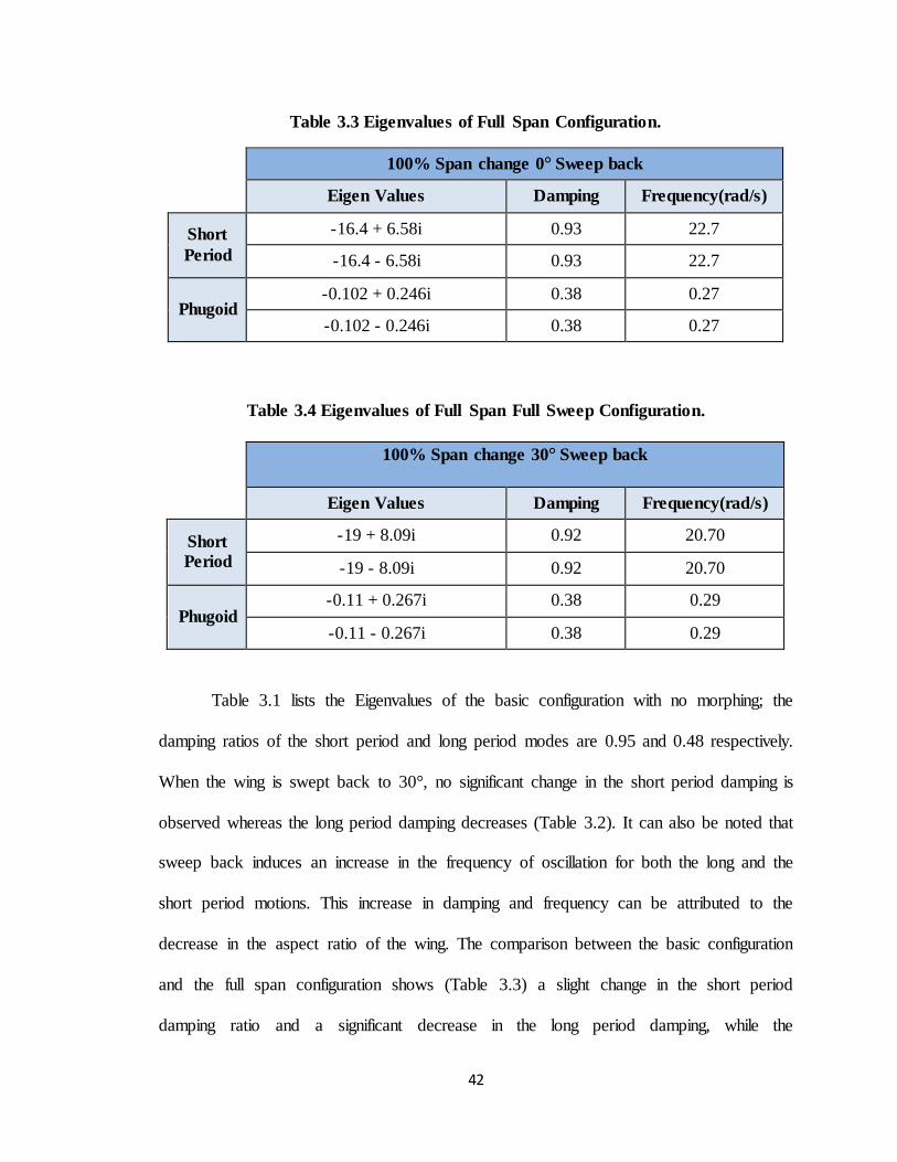
Table 3.3 Eigenvalues of Full Span Configuration.
100% Span change 0° Sweep back
Eigen Values Damping Frequency(rad/s)
Short
Period
-16.4 + 6.58i 0.93 22.7
-16.4 - 6.58i 0.93 22.7
Phugoid -0.102 + 0.246i 0.38 0.27
-0.102 - 0.246i 0.38 0.27
Table 3.4 Eigenvalues of Full Span Full Sweep Configuration.
100% Span change 30° Sweep back
Eigen Values Damping Frequency(rad/s)
Short
Period
-19 + 8.09i 0.92 20.70
-19 - 8.09i 0.92 20.70
Phugoid -0.11 + 0.267i 0.38 0.29
-0.11 - 0.267i 0.38 0.29
Table 3.1 lists the Eigenvalues of the basic configuration with no morphing; the
damping ratios of the short period and long period modes are 0.95 and 0.48 respectively.
When the wing is swept back to 30°, no significant change in the short period damping is
observed whereas the long period damping decreases (Table 3.2). It can also be noted that
sweep back induces an increase in the frequency of oscillation for both the long and the
short period motions. This increase in damping and frequency can be attributed to the
decrease in the aspect ratio of the wing. The comparison between the basic configuration
and the full span configuration shows (Table 3.3) a slight change in the short period
damping ratio and a significant decrease in the long period damping, while the

43
frequencies show incremental changes. Table 3.4 lists the eigenvalues, damping ratios
and frequencies of the short period and long period modes of the extended span and full
sweep back configuration.
Although SURFACES is a reliable preliminary analysis tool, the drag model
obtained from the low Reynold’s number conditions can be erroneous. This can be
observed while analyzing the modes of the aircraft. The high damping ratios and
frequency indicate higher drag than would be observed for a conventional aircraft of this
design. It was observed that increasing drag in the model caused the long period
(phugoid) Eigenvalues to move towards the real axis and eventually the imaginary part
would vanish with ample increase in drag. This caused the MAV to have a non-
oscillatory long period motion with high damping.
3.3 CONTROLLER DESIGN
A longitudinal stability augmentation system (SAS) was designed to control the
MAV during morphing. Changing the wing span and/or sweep changes the trim
conditions of the aircraft and, unless the system is altered by applying control inputs are
applied, results in a change in altitude. The purpose of the SAS control system therefore
was to enable the MAV to achieve constant-altitude trim conditions after morphing.
The SAS control system is designed as a state feedback controller ∆𝑈 = [−𝐾]∆𝑋,
here [K] is constant gain matrix. Substituting this control law into the linear state
equation yields
∆X=[A]∆X+[B]∆U
=[A]∆X-[B] [K] ∆X
= [A-BK] ∆X
44
=[A] ∆X
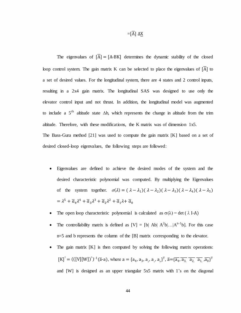
The eigenvalues of [A] = [A-BK] determines the dynamic stability of the closed
loop control system. The gain matrix K can be selected to place the eigenvalues of [A] to
a set of desired values. For the longitudinal system, there are 4 states and 2 control inputs,
resulting in a 2x4 gain matrix. The longitudinal SAS was designed to use only the
elevator control input and not thrust. In addition, the longitudinal model was augmented
to include a 5th altitude state h, which represents the change in altitude from the trim
altitude. Therefore, with these modifications, the K matrix was of dimension 1x5.
The Bass-Gura method [21] was used to compute the gain matrix [K] based on a set of
desired closed-loop eigenvalues, the following steps are followed:
Eigenvalues are defined to achieve the desired modes of the system and the
desired characteristic polynomial was computed. By multiplying the Eigenvalues
of the system together. (𝜆) = ( 𝜆 − 𝜆1)( 𝜆 − 𝜆2)( 𝜆− 𝜆3)( 𝜆 − 𝜆4)( 𝜆 − 𝜆5)
= 𝜆5 + 𝑎4𝜆4 + 𝑎3𝜆3 + 𝑎2𝜆2 + 𝑎1𝜆+ 𝑎0
The open loop characteristic polynomial is calculated as (λ) = det (λI-A)
The controllability matrix is defined as [V] = [b| Ab| A2b|…|An-1b]. For this case
n=5 and b represents the column of the [B] matrix corresponding to the elevator.
The gain matrix [K] is then computed by solving the following matrix operations:
[K]T = (([V][W])
T)-1(a-a), where a = a4, a3, a
2, a
1, a
0T, a=a4, a3, a2, a1, ,a0T
and [W] is designed as an upper triangular 5x5 matrix with 1’s on the diagonal

45
and coefficients of the desired characteristic polynomials a4, a3, a2, a
1, a
0 on the
super diagonal.
In the nonlinear simulation model, the SAS is implemented as a feedback loop
involving the forward velocity (u), altitude, vertical velocity (w), pitch rate (q) and pitch
angle (θ). The required trim values are subtracted from the current simulation values to
form an error vector ∆u, ∆w, ∆q, ∆θ, ∆hT, which represents the deviation from the
desired trim state. This error vector is then multiplied by the gain matrix [K] to obtain an
elevator deflection, which is added to the trim elevator deflection for the corresponding to
the desired trim state; this serves as the control effort outputted to the aircraft. SAS
control systems were designed to drive the aircraft to full span trim condition and the full
sweep trim condition. For example, the full span SAS implemented in the case where the
aircraft morphs from the baseline (zero span increase, zero sweep angle) configuration to
the full span configuration in order to trim the aircraft at the same altitude after the span
change occurs.
3.4 SIMULATION RESULTS AND ANALYSIS
A series of simulation studies were performed in which the wing span and/or
sweep were varied at different morphing rates. In each simulation the aircraft starts with
the baseline configuration (i.e. zero span increase, zero sweep angle) at the calculated
trim condition. The aircraft flies at this trim for the first 10 seconds of the simulation. The
morphing starts at the 11th second and lasts till for a specified time depending on the
morphing rate required. The altitude, angle of attack, total airspeed, pitch rate and pitch
angle are then plotted v/s time for all the different morphing rates in order to analyze the
46
dynamics associated with morphing. Several open-loop morphing (i.e. no control system
used) morphing cases are presented in order to demonstrate the effects of morphing.
Simulations results are then provided using the stability augmentation control system.
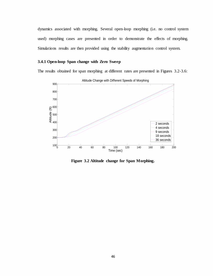
3.4.1 Open-loop Span change with Zero Sweep
The results obtained for span morphing at different rates are presented in Figures 3.2-3.6:
Figure 3.2 Altitude change for Span Morphing.
0 20 40 60 80 100 120 140 160 180 200100
200
300
400
500
600
700
800
900
Time (sec)
Altitu
de
(ft
)
Altitude Change with Different Speeds of Morphing
2 seconds
4 seconds
9 seconds
18 seconds
36 seconds

47
Figure 3.3 Angle of Attack change for Span Morphing.
Figure 3.4 Airspeed change for Span Morphing.
0 20 40 60 80 100 120 140 160 180 200-1
-0.8
-0.6
-0.4
-0.2
0
0.2
0.4
Time (sec)
An
gle
of
Att
ack
(de
g)
Change in Angle of Attack with different Speeds of Morphing
2 seconds
4 seconds
9 seconds
18 seconds
36 seconds
0 20 40 60 80 100 120 140 160 180 20042
44
46
48
50
52
54
56
58
60
62
Time (sec)
Air
sp
ee
d (
ft/s
)
Airspeed Change with Different Speeds of Morphing
2 seconds
4 seconds
9 seconds
18 seconds
36 seconds

48
Figure 3.5 Pitch Rate change for Span Morphing.
Figure 3.6 Pitch Angle change for Span Change.
Increasing the span, as discussed in the previous sections, causes an increase in
the total lift generated by the aircraft. Figure 3.2 plots the change in altitude v/s time
while span changes. The morphing begins at the 11th second and continues for 2, 4, 9, 18
and 36 seconds. These five cases are plotted against each other to observe the trend. It
0 20 40 60 80 100 120 140 160 180 200-1.5
-1
-0.5
0
0.5
1
1.5
2
Time (sec)
Pitch
Ra
te
(de
g/s
ec)
Pitch Rate Change with Different Speeds of Morphing
2 seconds
4 seconds
9 seconds
18 seconds
36 seconds
0 20 40 60 80 100 120 140 160 180 200-1
0
1
2
3
4
5
6
7
8
9
Time (sec)
Pitch
(de
g)
Pitch Angle Change with different speeds of Morphing
2 seconds
4 seconds
9 seconds
18 seconds
36 seconds
49
can be seen that the aircraft finds a new trim in climb after the span has changed; it is
interesting to note that the rate of climb is not affected by the speed of morphing although
the slower morphing cases trim into the climb with a delay thus creating a slight offset.
Figure 3.3 plots the angle of attack change v/s time, from which it is evident that
oscillatory motion occurs in the faster cases. It can also be observed that the faster
morphing cases cause the larger amplitude of oscillations; this is an important fact to
consider as a more stable flight can be achieved with larger morphing durations as almost
all the different cases damp out at about the same time. Figure 3.4 plots the Airspeed
change for the span change, the same trends as angle of attack can be observed. The
airspeed trims at a lower value than the initial trim; this is because the aircraft is now in a
climbing trim condition. Similar trends are observed pitch rate (Figure 3.5) and pitch
angle (Figure 3.6) although the pitch rate dampens out to zero while the pitch angle
settles to a positive angle corresponding to a climb.
3.4.2 Open-loop Sweep change with Zero Span increase
Figures 3.7-3.11 illustrate the simulation results for the case in which the wing is
morphed into a full (30° sweep back) sweep configuration with no span change. Results
provided for different morphing rates corresponding to 2, 4, 9, 18 and 36 seconds.
The morphing begins at the 11th second and continues for 2, 4, 9, 18 and 36
seconds. Sweep change decreases the overall lift of the aircraft; this can be observed in
the plot representing Altitude change (Figure 3.7) for sweep change. The MAV finds a
trim in descent as opposed to climb as in the previous (span morphing) case. These five
cases are plotted against each other to observe the trend. It can be seen that the aircraft
finds a trim in descent after the sweep has changed; it is interesting to note that the rate of

50
climb is not affected by the speed of morphing although the slower morphing cases trim
into the descent with a delay thus creating a slight offset. The Angle of Attack trims to a
higher value for all the different speeds in approximately the same amount of time
(Figure 3.8), however the airspeed (Figure 3.9) increases a little due to the trim found in
descent, the trends appear to be consistent with the previous cases. Figure 3.10 and 3.11
depict the pitch rate and pitch angle respectively, it can be observed here that the pitch
rate dampens to a zero value from a negative pitch rate. This results in a negative aircraft
pitch angle to point down and finding a negative trim angle which corresponds to a
descent trim condition.
Figure 3.7 Altitude Change for Sweep Morphing.
0 20 40 60 80 100 120 140 160 180 200-150
-100
-50
0
50
100
150
200
250
Time (sec)
Altitu
de
(ft)
Altitude Change for Different Speeds of Morphing
2 seconds
4 seconds
9 seconds
18 seconds
36 seconds

51
Figure 3.8 Angle of Attack change for Sweep Morphing.
Figure 3.9 Airspeed change for Sweep Morphing.
0 20 40 60 80 100 120 140 160 180 200-0.35
-0.3
-0.25
-0.2
-0.15
-0.1
-0.05
0
0.05
Time (sec)
An
gle
of
Att
ack
(de
g)
AoA Change with Different Speeds of Morphing
2 seconds
4 seconds
9 seconds
18 seconds
36 seconds
0 20 40 60 80 100 120 140 160 180 20057
57.5
58
58.5
59
59.5
60
60.5
61
61.5
62
Time (sec)
Air
sp
ee
d (
ft/s
)
Airspeed Change with Different Speeds of Morphing
2 seconds
4 seconds
9 seconds
18 seconds
36 seconds

52
Figure 3.10 Pitch Rate change for Sweep Morphing.
Figure 3.11 Pitch Angle change for Sweep Morphing.
0 20 40 60 80 100 120 140 160 180 200-0.8
-0.6
-0.4
-0.2
0
0.2
0.4
0.6
Time (sec)
Pitch
Ra
te (
de
g/s
)
Pitch Rate Change with Different Speeds of Morphing
2 seconds
4 seconds
9 seconds
18 seconds
36 seconds
0 20 40 60 80 100 120 140 160 180 200-3
-2.5
-2
-1.5
-1
-0.5
0
0.5
1
Time (sec)
Pitch
(d
eg
)
Pitch Change with Different Speeds of Morphing
2 seconds
4 seconds
9 seconds
18 seconds
36 seconds

53
3.4.3 Open-loop Span and Sweep Morphing
A set of open-loop simulations were performed in which the span and sweep were
changed at the same time at varying morphing rates, the results of which are presented in
Figures 3.12-3.16.
Expanding the span and sweeping the wings back brings about a few changes that
are difficult to perceive without the dynamic simulations. The overall lift on the aircraft
increases and the aircraft finds itself in a trim climb like the span only case, but in this
instance the rate of climb (Figure 3.12) is much lower than the one in observed in the
span only case (Figure 3.2). This observation can be attributed to the fact that while a
span increase causes an increment in the lift of the aircraft, sweep negates that effect to a
certain extent. The angle of attack increases slightly to a new trim value (Figure 3.13)
while the airspeed settles to a trim value which is lower than the initial trim (Figure 3.14);
it can also be observed that the airspeed trim for the sweep-span morphing case is less
than one noted in the span only case. Pitch rate (Figure 3.15) and pitch angle (Figure
3.16) follow similar trends as the previous cases, the pitch rate dies down to zero while
the pitch angle settles at a positive value indicating a nose up moment and therefore
climb.
It may be observed that the parameters observed in the above simulations settle to
a trim value almost within the same time frame, although it can be argued that the faster
morphing cases has more time to achieve equilibrium than the slower morphing
scenarios. This phenomenon merits further investigation.

54
Figure 3.12 Altitude change for Sweep and Span Morphing.
Figure 3.13 Angle of Attack change for Sweep and Span Morphing.
0 20 40 60 80 100 120 140 160 180 200200
250
300
350
400
450
Time (sec)
Att
itu
de
(ft
)
Altitude Change with Differnt Speeds of Morphing
2 seconds
4 seconds
9 seconds
18 seconds
36 seconds
0 20 40 60 80 100 120 140 160 180 200-0.4
-0.35
-0.3
-0.25
-0.2
-0.15
-0.1
-0.05
0
Time (sec)
An
gle
of
Att
ack (
de
g)
AoA Change with Different Speeds of Morphing
2 seconds
4 seconds
9 seconds
18 seconds
36 seconds

55
Figure 3.14 Airspeed change for Sweep and Span Morphing.
Figure 3.15 Pitch Rate change for Sweep and Span Morphing.
0 20 40 60 80 100 120 140 160 180 20055
56
57
58
59
60
61
Time (sec)
Tru
e A
irsp
ee
d (
ft/s
)
Airspeed Change with Different Morphing Speeds
2 seconds
4 seconds
9 seconds
18 seconds
36 seconds
0 20 40 60 80 100 120 140 160 180 200-0.5
0
0.5
1
Time (sec)
Pitch
Ra
te (
de
g/s
)
Pitch Rate Change with Different Speeds of Morphing
2 seconds
4 seconds
9 seconds
18 seconds
36 seconds

56
Figure 3.16 Pitch Angle change for Sweep and Span Morphing.
3.4.4 Closed Loop Control Cases
Figure 3.17 depicts the controller implemented to hold the altitude to 200 ft. for
the span morphing case; two separate scenarios were simulated for this report, morphing
was completed in 9 seconds for both cases. The first case depicts starting the altitude hold
after the span morphing has taken place, whereas the second case is using the altitude
hold as soon as the morphing starts. It can be inferred that the amplitude of oscillations is
considerably lowered when the control effort is applied as soon as the morphing starts.
Figure 3.18 is the implementation of the altitude hold for the sweep morphing case, the
morphing time is kept the same at 9 seconds for the 0 to 30° sweep. The results obtained
are similar to the ones observed in the span morphing scenario although the amplitude of
oscillation in this case is slightly larger and damping takes a longer amount of time.
0 20 40 60 80 100 120 140 160 180 200-0.5
0
0.5
1
1.5
2
2.5
3
Time (sec)
Pitch
(d
eg
)
Pitch Change with Differnt Speeds of Morphing
2 seconds
4 seconds
9 seconds
18 seconds
36 seconds
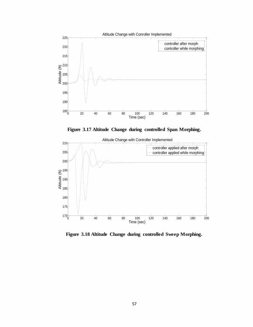
57
Figure 3.17 Altitude Change during controlled Span Morphing.
Figure 3.18 Altitude Change during controlled Sweep Morphing.
0 20 40 60 80 100 120 140 160 180 200185
190
195
200
205
210
215
220
225
Time (sec)
Altitu
de
(ft
)
Altitude Change with Conroller Implemented
controller after morph
controller while morphing
0 20 40 60 80 100 120 140 160 180 200170
175
180
185
190
195
200
205
210
Time (sec)
Altitu
de
(ft
)
Altitude Change with Controller Implemented
controller applied after morph
controller applied while morphing
58
CHAPTER 4: CONCLUSIONS
The objective of the thesis was to design and analyze a variable sweep, variable
span morphing MAV and study the transient characteristics morphing induces into the
dynamics of the vehicle. The research was based on the idea that the morphing
longitudinal dynamics could be modeled as a quasi-static system and the effects of rate of
morphing could be analyzed. This would help decipher optimal rates and trajectories of
morphing.
A carbon fiber reinforced Styrofoam model of a wing was constructed. This wing
was then instrumented with sensors for static and dynamic pressure measurements and
servo motor actuated mechanisms for varying the sweep and span of the aircraft were
developed. It was then tested in the wind tunnel to obtain the pressure variation during
morphing for different rates of sweep back and span increase. The static and dynamic
data collected were then analyzed to plot the pressure variation. Unfortunately, the data
collected were inconclusive for predicting the transient changes that take place during
morphing. The failure of the experiments could be attributed to an unstable open wind
tunnel with high degree of variation in the speeds of operation and the inability of the
data acquisition system to acquire the output at the sensitivity required for a successful
experiment. More details about the experimental design set up and testing is explained in
Appendix A.
A UAV model designed around the experimental wing was then modeled in a
Vortex Lattice Method solver named SURFACES. This software uses the user to input

59
geometrical parameters and weight distribution and creates panels that simulate the flow
over the surface. This three dimensional VLM solver outputs various aircraft properties
ranging from the moments and inertias to the center of gravity, neutral points and stick
fixed static margin. The software also provides us with aerodynamic coefficients and trim
solutions for a selected airspeed and altitude for any of the required axis. 77 different
models were created in SURFACES to represent every permutation of sweep and span
change between the initial and final span (with 0.06’ increments) and zero to 30° sweep
back (with 5° increments). The longitudinal aerodynamic coefficients were reported and
the trends for span and sweep change were analyzed.
6 degrees of freedom model was then built to simulate the non-linear dynamic
equations of an aircraft. This SIMULINK model was then modified to incorporate a
linear trajectory of sweep and span morphing at desired rates. Data obtained from
SURFACES for various configurations of the aircraft was interpolated to form data
tables, these tables serve as a reference to the non-linear model. For every time step
during change in sweep and/or span of the aircraft longitudinal aerodynamic coefficients
referenced for those particular configurations are fed into the model in real time. This
created a real time dynamic simulation used to study the change in the longitudinal
modes of the UAV.
The trim elevator deflection, trim angle of attack and trim thrust for the 4 end
configurations were calculated. The non-linear model was then linearized about these
trim conditions and a dynamic mode analysis on the 4 end static configurations was then
carried out (‘end configurations’ imply the configuration at which the aircraft
starts/finishes morphing). The eigenvalues for the zero span change-zero sweep back,

60
zero span change-full sweep back, full span change-zero sweep back and full span
change-30° sweep back were calculated and reported. Important dynamic data like the
frequency and damping of the oscillations of the two major longitudinal dynamic modes
i.e. the short period and the phugoid (long period) were reported and the effect of
geometrical changes on these parameters was highlighted.
A state feedback controller was then designed as a stability augmentation system
to enable the aircraft to maintain altitude throughout the flight. The Bass-Gura method
was used to calculate a gain matrix which was used to place the eigenvalues of the closed
loop system to optimum values desired. This gain matrix was then multiplied with the
feedback state errors to calculate the elevator deflections to maintain a constant altitude.
These simulations were run for five different rates of morphing 2, 4,9,18 and 36
seconds respectively. The longitudinal parameters like the forward velocity, angle of
attack, pitch rate, pitch angle and the altitude were plotted against time. The results were
analyzed and important trends were noted and discussed.
The thesis was successfully able to analyze and report the behavior of longitudinal
dynamics of a morphing aircraft with varying rates of change.
4.1 FUTURE SCOPE OF WORK
Although a substantial amount of work has been accomplished during the course of this
thesis, the author would like to propose some future research on this topic that can be
accomplished.
Re-conducting the experiments with dynamic pressure sensors and a stable wind
tunnel to obtain the dynamic changes that take place during morphing.
61
Analyzing the results of the experiments and building the intermediary transient
equations for the change of aerodynamic coefficients.
Studying different morphing trajectories like quadratic, parabolic etc., other than
the linear trajectory case analyzed in this report.
Model the lateral dynamic coefficients to analyze what effect morphing has on the
coupled modes.
Design a dynamic controller that actively computes the controller gains to control
the MAV.
Creating a Linear Time Varying (LTV) model to conduct modal analysis on
morphing dynamics.

62
APPENDIX A
A.1 DESIGN
The prototype wing is a simple rectangular wing design made from a GA (W)-1
airfoil. This section has a 12 inch chord length and a 21 inch base span. It is able to
increase its span to 25 inches and experiments were conducted on sweep change of up to
30 degrees. This prototype is depicted in Figure A.1.
Figure A.1 Wing Prototype.
To get the steady flow at low Reynolds numbers a laminar flow airfoil was
selected (GA (W)-1). It was then reinforced so that the flutter can be reduced to an
acceptable value at the speeds of operation required. Monokote, used as skin for wings
was tried, to reinforce the wing but was found to be too flimsy to hold the extended wing
section for span change. It was then decided that carbon fiber reinforcement would be
strong enough to suppress flutter and hold the extended wing.

63
The Styrofoam wing was built by the Imperial Foam and Insulation Mfr. by
means of a hot wire CNC. A CAD model of the airfoil shape and the dimensions were
provided and a Styrofoam model of the wing was obtained. Mounting units were drilled
onto the wing for mounting it to the wind tunnel’s force balance. The Styrofoam wing
was then treated with epoxy and cotton fiber slurry to help prevent the chances of epoxy
being soaked into the Styrofoam during the reinforcement process. This process was
repeated until a thin consistent layer of epoxy was obtained; the layer was left to settle for
an hour. A 1:2 mixture of epoxy to hardener was used to treat a 4 layer thick (0, +45,-45,
90) weave of carbon fiber. Two methods were investigated during this reinforcement:
reinforcing each side of the wing one at a time with two separate sheets of carbon fiber or
doing both sides at the same time with a single sheet. Treating both wing sides at the
same time gave a better finish to the final product as compared to doing it one at a time.
The final product obtained was sturdy and could withstand high winds and shear; it was
also able to support the extended wing but the surface finish obtained was not
satisfactory. Therefore, it was decided to try vacuum bagging with a porous peel ply to
obtain a smoother overall finish. The wing model was covered with a thin layer of epoxy
and a sheet of porous peel ply was set upon the epoxy. The wing was then sealed and a
vacuum setup. The vacuum helped the excess epoxy to get soaked by the peel ply and
give us an even finish. Although a smoother finish was obtained from the process the
model still needed to be sanded rigorously to obtain as close to a perfect finish as
possible, seven coats of polyurethane paint and more sanding was done. It was decided
that sanding was a never ending loop and mutual consensus was reached when a certain
level of finish was reached to stop sanding.
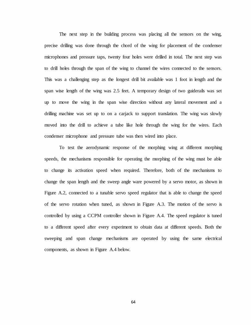
64
The next step in the building process was placing all the sensors on the wing,
precise drilling was done through the chord of the wing for placement of the condenser
microphones and pressure taps, twenty four holes were drilled in total. The next step was
to drill holes through the span of the wing to channel the wires connected to the sensors.
This was a challenging step as the longest drill bit available was 1 foot in length and the
span wise length of the wing was 2.5 feet. A temporary design of two guiderails was set
up to move the wing in the span wise direction without any lateral movement and a
drilling machine was set up to on a carjack to support translation. The wing was slowly
moved into the drill to achieve a tube like hole through the wing for the wires. Each
condenser microphone and pressure tube was then wired into place.
To test the aerodynamic response of the morphing wing at different morphing
speeds, the mechanisms responsible for operating the morphing of the wing must be able
to change its activation speed when required. Therefore, both of the mechanisms to
change the span length and the sweep angle ware powered by a servo motor, as shown in
Figure A.2, connected to a tunable servo speed regulator that is able to change the speed
of the servo rotation when tuned, as shown in Figure A.3. The motion of the servo is
controlled by using a CCPM controller shown in Figure A.4. The speed regulator is tuned
to a different speed after every experiment to obtain data at different speeds. Both the
sweeping and span change mechanisms are operated by using the same electrical
components, as shown in Figure A.4 below.

65
Figure A.2 Hitec-645MG
Ultra Torque Servo.
Figure A.3
Speed/Direction
Regulator.
Figure A.4 CCPM servo
controller.
A.2 METHODOLOGY
There were two primary sensors used, the pressure transducers and the condenser
microphones. These two sensors were plugged into the National Instruments USB-6008
Data Acquisition Board. The condenser microphones purchased from Radio Shack
operated with a 9V battery, a 100Ω resistor, and a 10mF capacitor. The sensitivity of the
device is -64±2dB. The signal/noise recognition of the condenser microphone is 50dB
minimum with a frequency response of 50-10,000Hz. The pressure transducers allow
input of pressure from the pressure taps and output alternating current to the DAQ board.
Finally, the National Instruments USB-6008 Data Acquisition Board accommodates four
channels of differential analog input channels, which allow for the adjustment of input
ranges. The analog input resolution is 12 bits differential with a maximum sample rate of
10kS/s (aggregate). Available input ranges in differential mode are ±1V, ±1.25V, ±2V,
±2.5V, ±4V, ±5V, ±10V, and ±20V. It is important to note that if single-ended analog
input is selected, 8 analog inputs are available but only a voltage input range of ±10V is
available.
The goal of this experiment was to find a suitable morphing speed that would be
optimal for sweep and span change. This was achieved by investigating the aerodynamic

66
properties of a morphing wing during the transition stage. An experimental procedure
was devised for the wing model in the wind tunnel. Before placing the test subject into
the wind tunnel to conduct experiments, a few tests were conducted to make sure that the
test devices work perfectly and gave the desired results. Tufts were also used in this test
to obtain the flow movement of the airfoil. All the flows were recorded using high-speed
camera and playback was done slow motion.
Constant pressure was used to perform the calibrations; the pressure taps, which
had constant pressure during calibration, were connected to the Data Acquisition (DAQ)
board. For every pressure value, there were five values that were collected to ensure the
consistency. It is important to note that the original plan of having twelve measurements
of pressure and transient response along the chord of the wing had to be changed due to
restrictions of the DAQ. Since there were only four channels available for adjusting the
input range, four locations of pressure and transient response were chosen based on
engineering judgment. Figure A.5 shows these four locations of measurement and the
subsequent omitted locations.

67
Figure A.5 Pressure Transducer/Condenser Microphone Locations.
The experiment began with the positioning of the test subject in the wind tunnel in
such a way that there was minimum interference. A full set of tests was performed with
the test object static in the initial position and the outcome was checked for
inconsistencies. Inconsistent or unreasonable results in the sample tests might occur
because of the sensors, the recording equipment, or the mounting of the test object. If
there were no inconsistent results from the sample tests, the experiment would proceed by
running a full set of tests with the test subject using varying sweep or span at different
angle of attack.
Experimental data was collected by varying the speed of sweep or span change at
different angles of attack (AoA). These measurements or parameters were collected as
pressure variation with respect to time. By using the pressure variation given by the
pressure transducer, aerodynamic coefficients and stability derivatives were then obtained
0.5, 0.64
6, 1.24
0.15, -0.24
6, -0.73
-1
-0.5
0
0.5
1
1.5
0 2 4 6 8 10 12
y-lo
cati
on
(in
)
Chord Location (in.)
8 Omitted Locations
4 Actual Locations
Station 1
Station 4
Station 7
Station 10
68
by plotting these variables against time, these can be used to determine the transient
characteristics brought about by morphing sweep and span separately.
A.3 RESULTS
First, the data from the Data Acquisition System (DAS) had to be compiled. Once
this was complete, the transient response during morphing was examined using the two
sets of data: pressure readings before and after morphing and the transient response
readings from the condenser microphones. As mentioned earlier, only four stations were
analyzed due to restrictions of the DAQ board.
A.3.1 Span Morphing
As stated before, for each angle of attack, five voltage measurements from the
pressure transducers for pre-morph and post-morph were taken. An average voltage from
the five samples was then taken. The pressure was then found by applying the respective
linear function of pressure vs. voltage from the calibration for each pressure transducer.
The resultant pressure is surface pressure minus ambient pressure (P- P∞). These pressure
values can be converted into the coefficient of pressure by using Eq. (1). Then,
subtracting the post-morph to pre-morph pressure, the change in Cp can be found.
CP=5.20232∆P
ρ∞ 𝑉∞2 (1)
where P is the surface pressure minus ambient pressure at a particular station as found
before (in.H2O), ∞
is density at ambient room temperature (70 °F) and pressure (33
in.H2O), which is 2.329E-3 slug/ft3 for the tests, and V∞ is the free stream velocity (25m/s
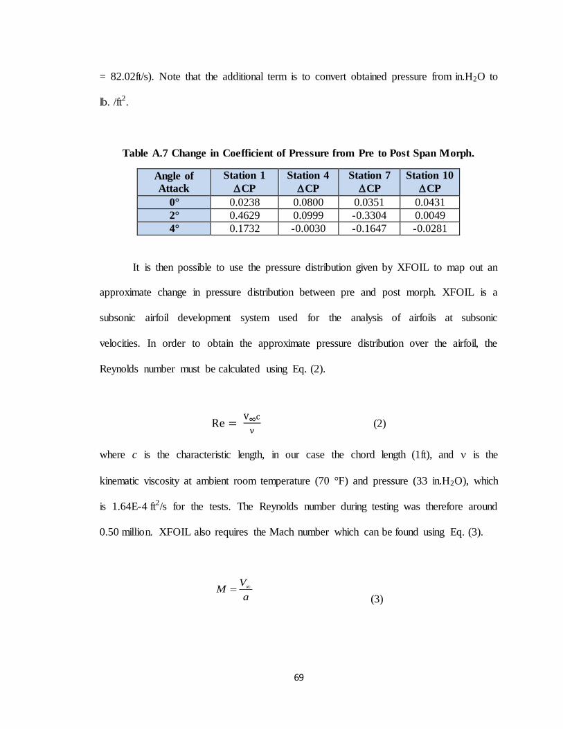
69
= 82.02ft/s). Note that the additional term is to convert obtained pressure from in.H2O to
lb. /ft2.
Table A.7 Change in Coefficient of Pressure from Pre to Post Span Morph.
Angle of
Attack
Station 1
CP
Station 4
CP
Station 7
CP
Station 10
CP
0° 0.0238 0.0800 0.0351 0.0431
2° 0.4629 0.0999 -0.3304 0.0049
4° 0.1732 -0.0030 -0.1647 -0.0281
It is then possible to use the pressure distribution given by XFOIL to map out an
approximate change in pressure distribution between pre and post morph. XFOIL is a
subsonic airfoil development system used for the analysis of airfoils at subsonic
velocities. In order to obtain the approximate pressure distribution over the airfoil, the
Reynolds number must be calculated using Eq. (2).
Re = V∞c
ν (2)
where c is the characteristic length, in our case the chord length (1ft), and is the
kinematic viscosity at ambient room temperature (70 °F) and pressure (33 in.H2O), which
is 1.64E-4 ft2/s for the tests. The Reynolds number during testing was therefore around
0.50 million. XFOIL also requires the Mach number which can be found using Eq. (3).
VM
a
(3)

70
where a is the speed of sound at ambient room temperature (1128 ft/s). Therefore, the
Mach number during testing was 0.073.
Using the values calculated above, XFOIL was used to calculate the pressure
distribution along the airfoil for all three angles of attack using the viscous calculation
option (See Appendix for XFOIL graphs). The coefficient of pressure values were then
plotted on the pressure distribution calculated in XFOIL to see the correlation.
Figure A.6 Results of Span Change at 0° AoA Plotted on XFOIL Pressure
Distribution.
-2
-1.8
-1.6
-1.4
-1.2
-1
-0.8
-0.6
-0.4
-0.2
0
0 2 4 6 8 10 12
Cp
Chord Location (in.)
XFOIL CpDistribution

71
Figure A.7 Results of Span Change at 2° AoA Plotted on XFOIL Pressure
Distribution.
Figure A.8 Results of Span Change at 4° AoA Plotted on XFOIL Pressure
Distribution.
Based on engineering judgment, the results should indicate a decrease in pressure
(overall shift up of the graph) at all locations since the elliptical lift distribution has
-2.5
-2
-1.5
-1
-0.5
0
0 2 4 6 8 10 12
Cp
Chord Location (in.)
XFOIL CpDistribution
-3
-2.5
-2
-1.5
-1
-0.5
0
0 2 4 6 8 10 12
Cp
Chord Location (in.)
XFOIL CpDistribution

72
shifted from ending near the pressure locations to a point farther away from the pressure
taps. This is represented perfectly for the zero angle of attack data; however, the data is
inconsistent at the other angles of attack. In other words, the span change does not show a
consistent change in pressure distribution. It can be concluded that possible sources of
this error may be that the pressure transducer/DAQ board set-up is inadequate (possibly
due to insufficient calibration) to provide accurate results, or that the variations in the
open wind tunnel, with its fluctuations in speed and occasional gusts.
A.3.2 Sweep Morphing
Again, at each angle of attack, five voltage measurements from the pressure
transducers for pre-morph and post-morph were taken. An average voltage from the five
samples was then taken and the pressure was found by applying the respective linear
function of pressure vs. voltage from the calibration for each pressure transducer. The
resultant pressure is surface pressure minus ambient pressure (P-Pinf) which is denoted as
P in the tables below. These pressure values can be converted to coefficient of
pressure by using Eq. (1) and change in coefficient of pressure can be found by
subtracting post-morph from pre-morph data.
Table A. 8 Change in Coefficient of Pressure from Pre to Post Sweep Morph.
Angle of
Attack
Station 1
CP
Station 4
CP
Station 7
CP
Station 10
CP
0° 0.1144 -0.0172 -0.0764 -0.0478
2° 0.3063 0.1054 -0.1835 0.0086
4° 0.0271 0.0080 0.0696 -0.0006
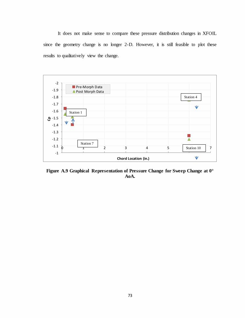
73
It does not make sense to compare these pressure distribution changes in XFOIL
since the geometry change is no longer 2-D. However, it is still feasible to plot these
results to qualitatively view the change.
Figure A.9 Graphical Representation of Pressure Change for Sweep Change at 0°
AoA.
-2
-1.9
-1.8
-1.7
-1.6
-1.5
-1.4
-1.3
-1.2
-1.1
-1
0 1 2 3 4 5 6 7
Cp
Chord Location (in.)
Pre-Morph DataPost Morph Data
Station 1
Station 4
Station 7
Station 10
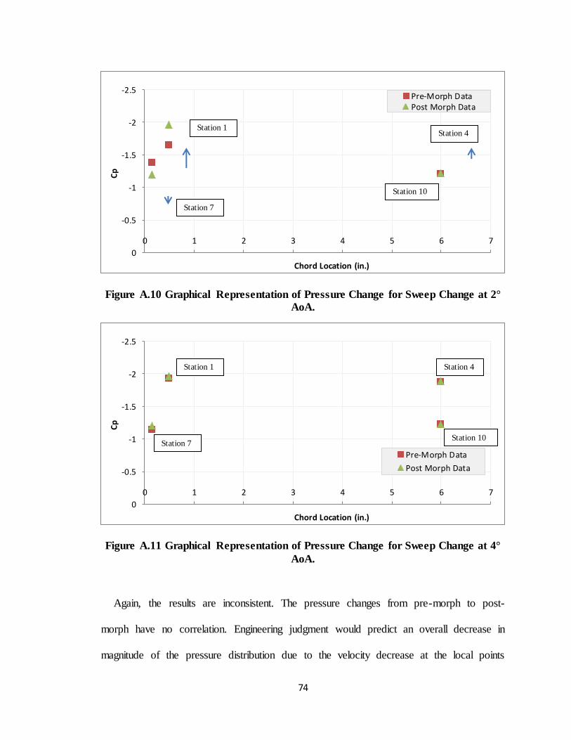
74
Figure A.10 Graphical Representation of Pressure Change for Sweep Change at 2°
AoA.
Figure A.11 Graphical Representation of Pressure Change for Sweep Change at 4°
AoA.
Again, the results are inconsistent. The pressure changes from pre-morph to post-
morph have no correlation. Engineering judgment would predict an overall decrease in
magnitude of the pressure distribution due to the velocity decrease at the local points
-2.5
-2
-1.5
-1
-0.5
0
0 1 2 3 4 5 6 7
Cp
Chord Location (in.)
Pre-Morph DataPost Morph Data
-2.5
-2
-1.5
-1
-0.5
0
0 1 2 3 4 5 6 7
Cp
Chord Location (in.)
Pre-Morph Data
Post Morph Data
Station 1 Station 4
Station 7
Station 10
Station 1 Station 4
Station 10 Station 7
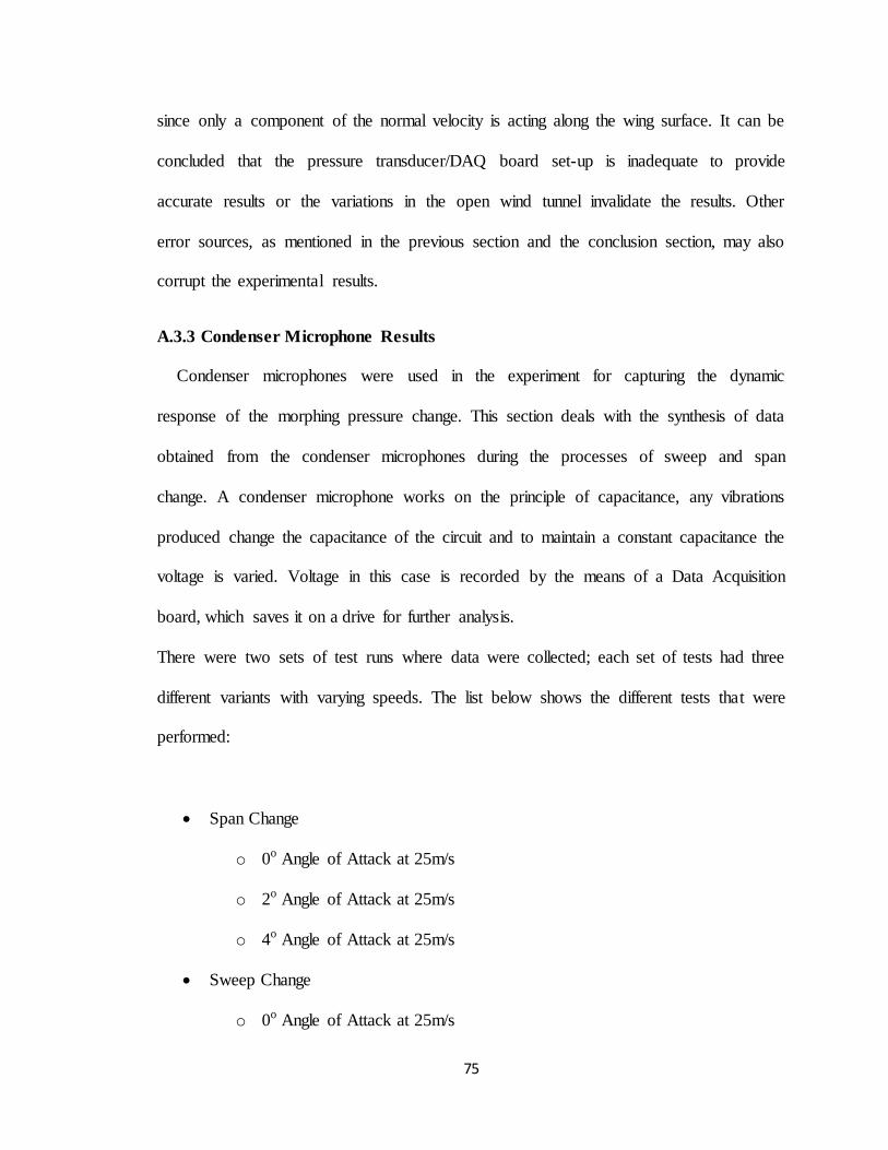
75
since only a component of the normal velocity is acting along the wing surface. It can be
concluded that the pressure transducer/DAQ board set-up is inadequate to provide
accurate results or the variations in the open wind tunnel invalidate the results. Other
error sources, as mentioned in the previous section and the conclusion section, may also
corrupt the experimental results.
A.3.3 Condenser Microphone Results
Condenser microphones were used in the experiment for capturing the dynamic
response of the morphing pressure change. This section deals with the synthesis of data
obtained from the condenser microphones during the processes of sweep and span
change. A condenser microphone works on the principle of capacitance, any vibrations
produced change the capacitance of the circuit and to maintain a constant capacitance the
voltage is varied. Voltage in this case is recorded by the means of a Data Acquisition
board, which saves it on a drive for further analysis.
There were two sets of test runs where data were collected; each set of tests had three
different variants with varying speeds. The list below shows the different tests that were
performed:
Span Change
o 0o Angle of Attack at 25m/s
o 2o Angle of Attack at 25m/s
o 4o Angle of Attack at 25m/s
Sweep Change
o 0o Angle of Attack at 25m/s

76
Slow sweep change
Snap sweep change
o 2o Angle of Attack at 25m/s
Slow sweep change
Snap sweep change
o 4o Angle of Attack at 25m/s
Slow sweep change
Snap sweep change
Multiple runs of these data sets were collected and were first visually inspected to
locate any noticeable change. As can be observed from Fig. 17, although there is no
easily discernable change noticed at around 3 seconds, there is a change in amplitude of
the signal. A Power Spectral Density plot was obtained to find that there was a dominant
frequency at 60 Hz with harmonics at 120 and 180 Hz respectively, which could be
attributed to AC noise. To further investigate these data, the specific time period was cut
and plotted; the data was then passed through a stop-band filter to eliminate the AC
frequency and harmonics. A low pass filter was used to eliminate the unwanted high
frequencies as it was determined that any transient pressure change would occur at
relatively low frequencies close to the frequency of morphing. Figure A.12 illustrates the
data signal obtained from these filters.
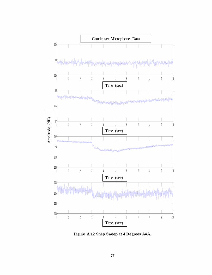
77
Figure A.12 Snap Sweep at 4 Degrees AoA.
0 1 2 3 4 5 6 7 8 9 103.25
3.3
3.35Condenser Microphone1
0 1 2 3 4 5 6 7 8 9 100.7
0.75
0.8Condenser Microphone2
0 1 2 3 4 5 6 7 8 9 102.36
2.38
2.4
2.42Condenser Microphone3
0 1 2 3 4 5 6 7 8 9 102.33
2.34
2.35
2.36Condenser Microphone4
Time (sec)
Am
plit
ude
(dB
)
Time (sec)
Time (sec)
Time (sec)
Condenser Microphone Data
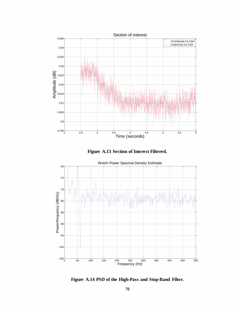
78
Figure A.13 Section of Interest Filtered.
Figure A.14 PSD of the High-Pass and Stop-Band Filter.
2 2.5 3 3.5 4 4.5 5 5.5 60.795
0.8
0.805
0.81
0.815
0.82
0.825
0.83
0.835
0.84
0.845
Section of interest
Time (seconds)
Am
plit
ud
e (
dB
)
STOPBAND FILTER
LOWPASS FILTER
0 50 100 150 200 250 300 350 400 450 500-105
-100
-95
-90
-85
-80
-75
-70
-65
Frequency (Hz)
Pow
er/
frequency (
dB
/Hz)
Welch Power Spectral Density Estimate

79
Unfortunately, there are no substantial results that can be derived about the
changes that occur during morphing from the obtained data. This stems from the fact that
the DAQ board and condenser microphone combination used could not measure the
minute changes in frequency which occur during the morphing transition. The NI USB-
6008 was programmed for the best input range; however if the data exceeded the input
range, no data were collected, which resulted in setting the DAQ to a higher input range,
which did not collect the data as desired. This particular setback was detrimental to the
data obtained and the required frequencies could not be captured. Some other flaws in the
experimental setup were noticed: the sensitivity of Condenser microphones to ambient
noise such as capturing the AC current frequency (the pressure transducer had to be
turned off during the data collection to avoid superimposition), flutter of the wing was
another issue that needed to be addressed even with dampened hinges, the flutter was
high enough to be captured by the microphones in the 5-15 Hz range. This was
particularly interesting to decipher in the data, during sweep change the hinge provided a
moment to the wing to sweep it against the hinge; although great care was taken to have
straight rods connecting the servo to the wing, there was still a vertical force provided by
the rod that induced peak flutter. This phenomenon can be observed right at the start of
morphing around 3 seconds (Figure A.13) into the experiment. PSD plots of the data
reveal dominant frequencies of around 13.7 Hz (Figure A.14), which could be attributed
to flutter.
The author found that the wind tunnel used for experimentation was not stable
enough for dynamic testing. There was dynamic response captured by the condenser
microphones, but the cause of the change could have been either the changing velocity or

80
the geometrical changes. The frequency of both of these changes was of the same order
of magnitude; therefore no classifications could be made. Although this experiment was
unsuccessful, the author firmly believes this method can be modified and used in future
testing of this kind.

81
Appendix B
Figure B.1 Calibration of Pressure Transducer Used at Station 4.
Figure B.2 Calibration of Pressure Transducer Used at Station 7.
y = 141.62x - 313.77 R² = 0.9996
0
0.5
1
1.5
2
2.5
3
3.5
4
2.21 2.215 2.22 2.225 2.23 2.235 2.24 2.245 2.25
Pre
ssu
re (
in.H
2O
)
Voltage
Pressure Transducer 4 Calibration
y = 137.91x - 306.28 R² = 0.9994
0
0.5
1
1.5
2
2.5
3
3.5
4
2.215 2.22 2.225 2.23 2.235 2.24 2.245 2.25 2.255
Pre
ssu
re (
in.H
2O
)
Voltage
Pressure Transducer 7 Calibration

82
Figure B.3 Calibration of Pressure Transducer Used at Station 10.
Figure B.4 Electronics.
y = 131.19x - 292.19 R² = 0.9988
0
0.5
1
1.5
2
2.5
3
3.5
4
4.5
2.22 2.225 2.23 2.235 2.24 2.245 2.25 2.255 2.26
Pre
ssu
re (
in.H
2O
)
Voltage
Pressure Transducer 10 Calibration
Battery packs Controller
Speed regulator
Connected to servo
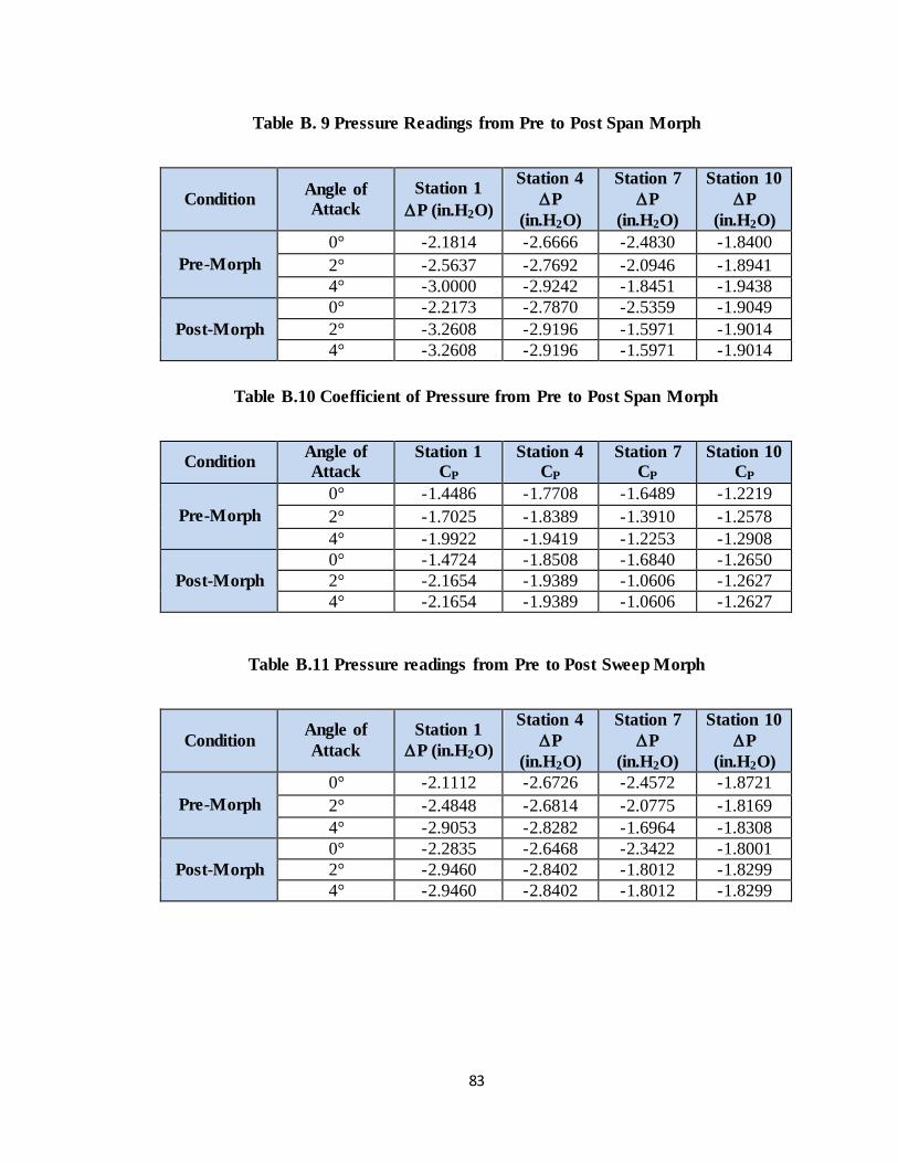
83
Table B. 9 Pressure Readings from Pre to Post Span Morph
Condition Angle of
Attack
Station 1
P (in.H2O)
Station 4
P
(in.H2O)
Station 7
P
(in.H2O)
Station 10
P
(in.H2O)
Pre-Morph
0° -2.1814 -2.6666 -2.4830 -1.8400
2° -2.5637 -2.7692 -2.0946 -1.8941
4° -3.0000 -2.9242 -1.8451 -1.9438
Post-Morph
0° -2.2173 -2.7870 -2.5359 -1.9049
2° -3.2608 -2.9196 -1.5971 -1.9014
4° -3.2608 -2.9196 -1.5971 -1.9014
Table B.10 Coefficient of Pressure from Pre to Post Span Morph
Condition Angle of
Attack
Station 1
CP
Station 4
CP
Station 7
CP
Station 10
CP
Pre-Morph
0° -1.4486 -1.7708 -1.6489 -1.2219
2° -1.7025 -1.8389 -1.3910 -1.2578
4° -1.9922 -1.9419 -1.2253 -1.2908
Post-Morph
0° -1.4724 -1.8508 -1.6840 -1.2650
2° -2.1654 -1.9389 -1.0606 -1.2627
4° -2.1654 -1.9389 -1.0606 -1.2627
Table B.11 Pressure readings from Pre to Post Sweep Morph
Condition Angle of
Attack
Station 1
P (in.H2O)
Station 4
P
(in.H2O)
Station 7
P
(in.H2O)
Station 10
P
(in.H2O)
Pre-Morph
0° -2.1112 -2.6726 -2.4572 -1.8721
2° -2.4848 -2.6814 -2.0775 -1.8169
4° -2.9053 -2.8282 -1.6964 -1.8308
Post-Morph
0° -2.2835 -2.6468 -2.3422 -1.8001
2° -2.9460 -2.8402 -1.8012 -1.8299
4° -2.9460 -2.8402 -1.8012 -1.8299
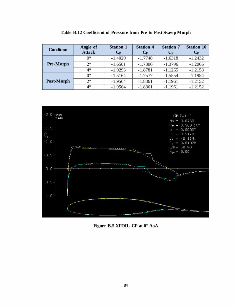
84
Table B.12 Coefficient of Pressure from Pre to Post Sweep Morph
Condition Angle of
Attack
Station 1
CP
Station 4
CP
Station 7
CP
Station 10
CP
Pre-Morph
0° -1.4020 -1.7748 -1.6318 -1.2432
2° -1.6501 -1.7806 -1.3796 -1.2066
4° -1.9293 -1.8781 -1.1265 -1.2158
Post-Morph
0° -1.5164 -1.7577 -1.5554 -1.1954
2° -1.9564 -1.8861 -1.1961 -1.2152
4° -1.9564 -1.8861 -1.1961 -1.2152
Figure B.5 XFOIL CP at 0° AoA

85
Figure B.6 XFOIL Pressure Distribution at 0° AoA
Figure B.7 XFOIL CP at 2° AoA
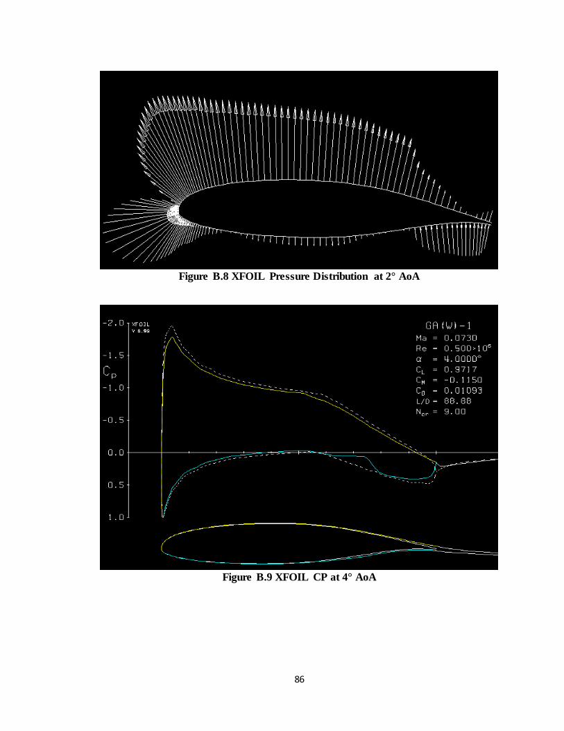
86
Figure B.8 XFOIL Pressure Distribution at 2° AoA
Figure B.9 XFOIL CP at 4° AoA

87
Figure B.10 XFOIL Pressure Distribution at 4° AoA

88
Bibliography
[1] M. Abdulrahim, H. Garcia, J. Dupuis and R. Lind, "Flight characterstics of a wing shaping for
a micro air vehicle with membrane wings," UF, Gainsville , 2004.
[2] Gevers Aircraft Inc, "Gevers Aircraft, Inc. Genesis," Gevers Aircraft, [Online]. Available:
http://www.geversaircraft.com/.
[3] J. S. Flanagan, R. C. Strutzenburg, R. B. Myers and J. E. Rodrian, "Development and Flight
Testing of a Morphing Aircraft," in AIAA/ASME/ASCE/AHS/ASC Structures, Structural
Dynamics and Materials Conference , Honolulu, Hawaii, 2007.
[4] A. Jha and J. Kudva, "Morphing Aircraft Concepts, Classification and Challenges," in NextGen
Aeronautics Inc., Torrance, CA, 2004.
[5] Gizmodo, "Gizmodo," [Online]. Available: Gizmodo.com.
[6] S. Barbarino, O. Bilgen, R. M. Ajaj, M. I. Friswell and D. J. Inman, "A Review of Morphing
Aircraft," Journal of Intelligent Material System and Structures , vol. 22, pp. 823-877, June-
2011.
[7] T. A. Weisshaar, "Morphing Aircraft Technology- New shapes for Aircraft Design," in
Multifunction structures/ Integration of sensor ANtennas, West Lafayette, IN , 2006.
[8] A. Chakravarthy, D. T. Grant and R. Lind, "Time-Varying Dynamics of a Micro Air Vehicle
with Variable-Sweep Morphing," Journal of Guidance, Control and Dynamics, vol. 35, no. 3,
p. 890, 2012.
[9] F. L. Engineering, "Surfaces," 2012. [Online]. Available:
http://www.flightlevelengineering.com/surfaces.
[10] P. Lizzy, "Live Science," 21 May 2013. [Online]. Available:
http://www.livescience.com/34569-why-flowers-close-at-night-nyctinasty.html.
[11] E. Stanewsky, "Adaptive Wing and Flow Control Technology," Progress in Aerospace Science
, pp. 583-667, 2001.
[12] O. Leon, E. Hayden and F. Gandhi, "Rotorcraft Operating Envelope Extension using
Extendable Chord Sections," in Proceedings of American Helicopter Society 65th Annual
Forum, Grapevine, Texas, 2009.

89
[13] P. Chen, D. Sarhaddi, R. Jha, D. Liu and K. Griffin, "Variable Stiffness Spar Approach for
Aircraft Maneuver Enhancement Using Astros," Journal of Aircraft 37, pp. 865-871, 2000.
[14] C. Nam, P. Chen, D. Sarhaddi, D. Liu, K. Griffin and R. Yurkovich, "Torsion-Free Wing
Concepts for Aircraft Maneuver Enhancement," in Proceedings of the 41st
AIAA/ASME/ASCE/AHS/ASC Structures, Structural Dynamics and Materials Conference,
Atlanta, GA, 2000.
[15] R. Guiler and W. Huebsch, "Wind Tunnel Analysis of a Morphing Swept Tailless Aircraft," in
Proceedings of 23rd AIAA Applied Aerodynamics Conference , Toronto , 2005.
[16] J. R. Florance, J. Hegg, C. V. Spain, T. G. Ivanco and C. D. Wieseman, "Variable Stiffness Spar
Wind-Tunnel Model Development and Testing," NASA Langley Research Center , Hampton,
VA.
[17] H. F. Parker, "The Parker Variable Camber Wing," Annual Report 77, National Advisory
Committee for Aeronautics , 1920.
[18] G. Sachs and R. Mehlhorn, "Endurance Increase by Periodic Optimal Camber Control,"
Journal of Guidance and Control Dynamics , pp. 572-578, 1993.
[19] W. Raither, L. D. Simoni, L. D. Lillo, A. Bergamini and P. Ermanni, "Adaptive-Twist Airfoil
Based on Electrostatic Stiffness Variation," in 22nd AIAA/ASME/AHS Adaptive Structures
Conference, National Harbor, 2014.
[20] I. H. AbbotInc and A. E. V. Doenhoff, Theory of Wing Sections, Dover Publication , 1958.
[21] R. C. Nelson, Flight Stbility and Automatic Control, McGraw Hill, 1998.
[22] E. Laitone, "Lift Curve Slope for Finite Aspect Ratio Wings," AIAA Proceeding Vol. 26 No. 8,
pp. 789-790, 1989.
[23] H. Garcia, M. Abdulrahim and R. Lind, "Roll control for a Micro Air Vehicle using Active wing
Morphing," University of Florida, Gainsville, 2002.
[24] J. S. Flanagan, R. C. Strutzenberg, R. B. Meyers and J. E. Rodrian, "Development and Flight
Testing of a morphing aircraft, the NextGen MFX-1," in 48th AIAA structures, Structural
Dynamics and Material Conference , Honolulu, Hawaii , 2007.
[25] Y. Zhao and H. Hu, "Prediction of transient responses of a folding wing during the morphing
process," Areospace Science and Technology, vol. 24, pp. 89-94, 2011.

90
[26] M. S. Selig, "Low reynolds number airfoil design," in Lecture notes , 2003.
[27] V. Burnelli, "Telescopically varying the airfoil camber and cord". USA Patent 1917428, 1933.
[28] R. Curry, "In flight total forces, Moments and static aeroelastic characterstics of an oblique
Wing Research Airplane," NASA AMES research ceneter, DRYDEN reseach facility, Edwards,
CA, 1984.
[29] T. Delft, "RoboSwift," TU Delft, 2007. [Online]. Available: http://www.roboswift.nl/.
[30] A. Ranjbar, M. Mehrabani and F. Pary, "Numerical Study on the Transient Response of a
Condenser Microphone," IEEE Sensors Journal, vol. 24, pp. 19-94, 2011.
[31] J. Blondeau, J. Richeson and D. J. Pines, "Design, development and testing of a morphing
aspect ratio wing using an inflatable telescopic spar," in 44th AIAA/ASME/ASCE/AHS
Structures, Structural Dynamics and Materials Conference, 7-10th April, 2003 .
[32] E. Jesse and J. Dijkstra, "Design study of a supersonic business jet with variable sweep
wings," in 27th Congress of Aeronautical Science , 19-24th September, 2010.
[33] R. Telgarsky, "Dominant Frequency Extraction," arXiv: 1306.0103v1, Albuquerque, New
Mexico, June 2013.