A Factored, Interpolatory Subdivision for Surfaces of Revolution
1
Design and Analysis of Multi-Factored Experiments
Engineering 9516g g
Dr. Leonard M. Lye, P.Eng, FCSCE, FECProfessor and Associate Dean (Graduate Studies)
Faculty of Engineering and Applied Science, Memorial University of Newfoundland
L. M. Lye DOE Course 1
NewfoundlandSt. John’s, NL, A1B 3X5
DOE - I
Introduction
L. M. Lye DOE Course 2
2
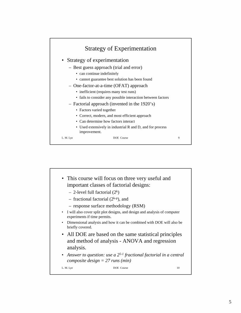
Design of Engineering ExperimentsIntroduction
• Goals of the course and assumptionsp• An abbreviated history of DOE• The strategy of experimentation• Some basic principles and terminology• Guidelines for planning, conducting and
L. M. Lye DOE Course 3
Guidelines for planning, conducting and analyzing experiments
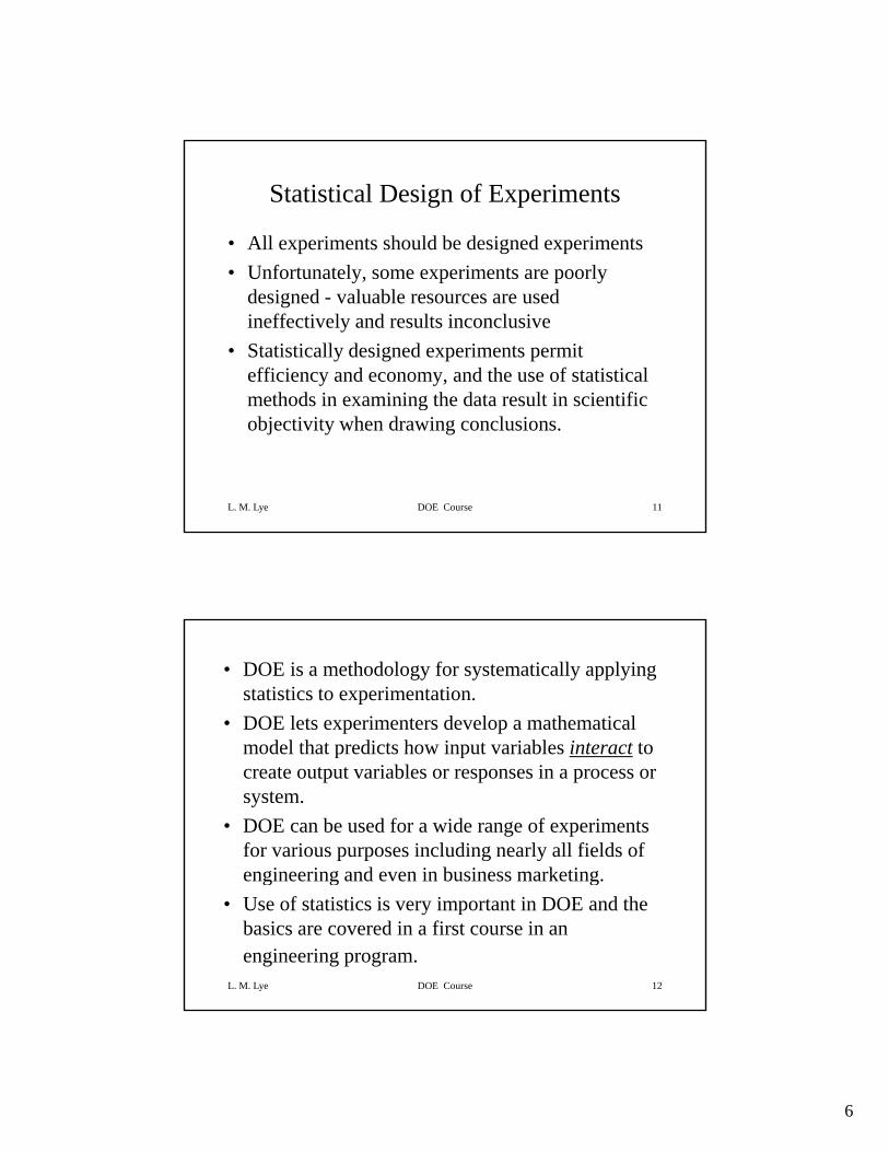
Assumptions• You have
– a first course in statistics– heard of the normal distribution– know about the mean and variance– have done some regression analysis or heard of it– know something about ANOVA or heard of it
• Have used Windows or Mac based computers
L. M. Lye DOE Course 4
• Have done or will be conducting experiments• Have not heard of factorial designs, fractional
factorial designs, RSM, and DACE.

3
Some major players in DOE
• Sir Ronald A. Fisher - pioneer – invented ANOVA and used of statistics in experimental
design hile orking at Rothamsted Agric lt raldesign while working at Rothamsted Agricultural Experiment Station, London, England.
• George E. P. Box - married Fisher’s daughter– still active (86 years old)– developed response surface methodology (1951)– plus many other contributions to statistics
L. M. Lye DOE Course 5
plus many other contributions to statistics• Others
– Raymond Myers, J. S. Hunter, W. G. Hunter, Yates, Montgomery, Finney, etc..
Four eras of DOE• The agricultural origins, 1918 – 1940s
– R. A. Fisher & his co-workers– Profound impact on agricultural science– Factorial designs, ANOVAg ,
• The first industrial era, 1951 – late 1970s– Box & Wilson, response surfaces– Applications in the chemical & process industries
• The second industrial era, late 1970s – 1990– Quality improvement initiatives in many companies– Taguchi and robust parameter design, process robustness
• The modern era beginning circa 1990
L. M. Lye DOE Course 6
The modern era, beginning circa 1990– Wide use of computer technology in DOE– Expanded use of DOE in Six-Sigma and in business– Use of DOE in computer experiments

4
References• D. G. Montgomery (2012): Design and Analysis
of Experiments, 8th Edition, John Wiley and Sons– one of the best book in the market. Uses Design-Expert g p
software for illustrations. Uses letters for Factors.• G. E. P. Box, W. G. Hunter, and J. S. Hunter
(2005): Statistics for Experimenters: An Introduction to Design, Data Analysis, and Model Building, John Wiley and Sons. 2nd Edition
L. M. Lye DOE Course 7
– Classic text with lots of examples. No computer aided solutions. Uses numbers for Factors.
• Journal of Quality Technology, Technometrics, American Statistician, discipline specific journals
Introduction: What is meant by DOE?• Experiment -
– a test or a series of tests in which purposeful changes are made to the input variables or factors of a system so that we may observe and identify the reasons forso that we may observe and identify the reasons for changes in the output response(s).
• Question: 5 factors, and 2 response variables– Want to know the effect of each factor on the response
and how the factors may interact with each other– Want to predict the responses for given levels of the
L. M. Lye DOE Course 8
p p gfactors
– Want to find the levels of the factors that optimizes the responses - e.g. maximize Y1 but minimize Y2
– Time and budget allocated for 30 test runs only.
5
Strategy of Experimentation
• Strategy of experimentation– Best guess approach (trial and error)
• can continue indefinitely• can continue indefinitely• cannot guarantee best solution has been found
– One-factor-at-a-time (OFAT) approach• inefficient (requires many test runs)• fails to consider any possible interaction between factors
– Factorial approach (invented in the 1920’s)F t i d t th
L. M. Lye DOE Course 9
• Factors varied together• Correct, modern, and most efficient approach• Can determine how factors interact• Used extensively in industrial R and D, and for process
improvement.
• This course will focus on three very useful and important classes of factorial designs: – 2-level full factorial (2k)– fractional factorial (2k-p), and – response surface methodology (RSM)
• I will also cover split plot designs, and design and analysis of computer experiments if time permits.
• Dimensional analysis and how it can be combined with DOE will also be briefly covered.
• All DOE are based on the same statistical principles d h d f l i ANOVA d i
L. M. Lye DOE Course 10
and method of analysis - ANOVA and regression analysis.
• Answer to question: use a 25-1 fractional factorial in a central composite design = 27 runs (min)
6
Statistical Design of Experiments
• All experiments should be designed experiments• Unfortunately some experiments are poorly• Unfortunately, some experiments are poorly
designed - valuable resources are used ineffectively and results inconclusive
• Statistically designed experiments permit efficiency and economy, and the use of statistical methods in examining the data result in scientific
L. M. Lye DOE Course 11
methods in examining the data result in scientific objectivity when drawing conclusions.
• DOE is a methodology for systematically applying statistics to experimentation.
• DOE lets experimenters develop a mathematical model that predicts how input variables interact tomodel that predicts how input variables interact to create output variables or responses in a process or system.
• DOE can be used for a wide range of experiments for various purposes including nearly all fields of engineering and even in business marketing.
L. M. Lye DOE Course 12
engineering and even in business marketing.• Use of statistics is very important in DOE and the
basics are covered in a first course in an engineering program.
7
• In general, by using DOE, we can:– Learn about the process we are investigating– Screen important variables p– Build a mathematical model– Obtain prediction equations– Optimize the response (if required)
L. M. Lye DOE Course 13
• Statistical significance is tested using ANOVA, and the prediction model is obtained using regression analysis.
Applications of DOE in Engineering Design
• Experiments are conducted in the field of engineering to:engineering to:– evaluate and compare basic design configurations– evaluate different materials– select design parameters so that the design will work
well under a wide variety of field conditions (robust design)
L. M. Lye DOE Course 14
– determine key design parameters that impact performance
8
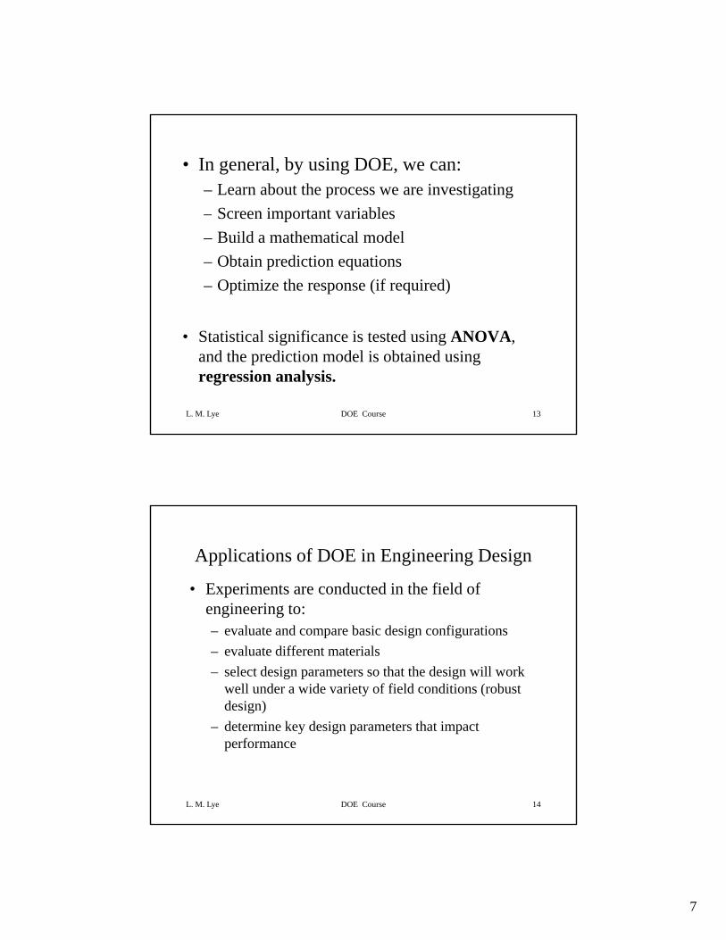
INPUTS(Factors)
X variables
OUTPUTS(Responses)Y variables
People
Materials
PROCESS:
A Blending of Inputs which Generates
Corresponding Outputs
Equipment
Policies
Procedures
responses related to performing a
service
responses related to producing a
produce
responses related to completing a task
L. M. Lye DOE Course 15
Outputs
Methods
Environment Illustration of a Process
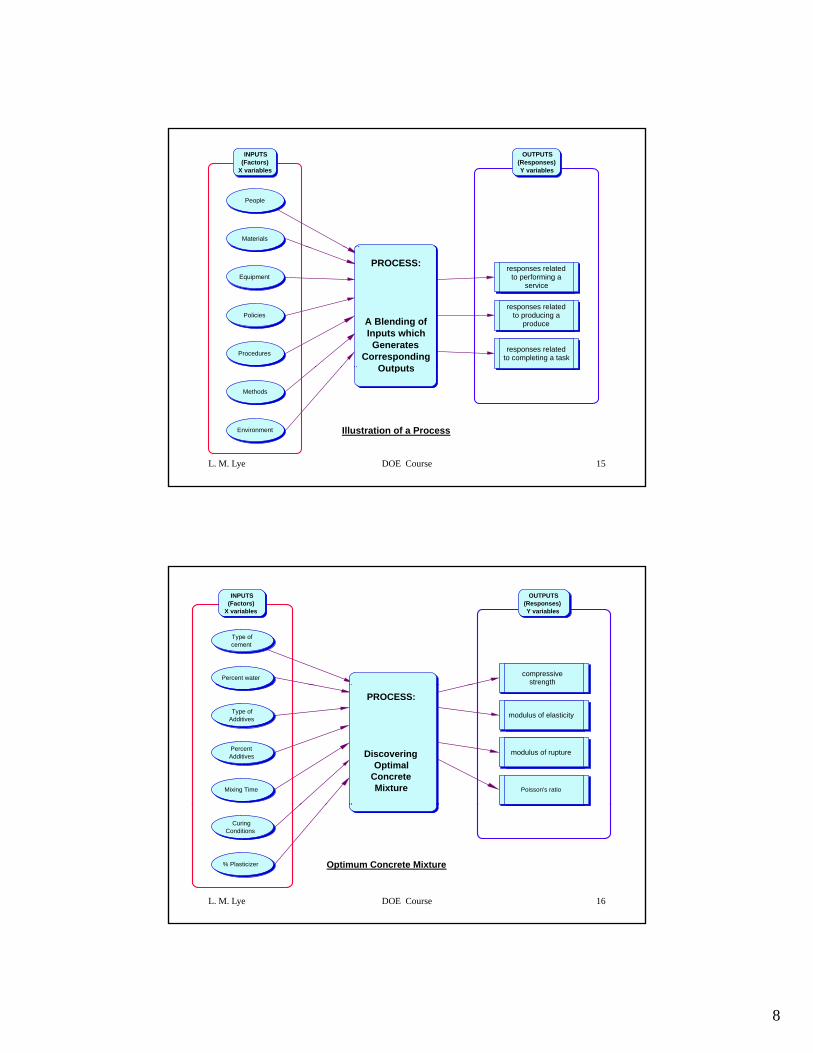
INPUTS(Factors)
X variables
OUTPUTS(Responses)Y variables
Type of cement
Percent water compressive strength
PROCESS:
Discovering Optimal
Concrete Mixture
Type of Additives
Percent Additives
Mixing Time
g
modulus of elasticity
modulus of rupture
Poisson's ratio
L. M. Lye DOE Course 16
Curing Conditions
% Plasticizer Optimum Concrete Mixture
9
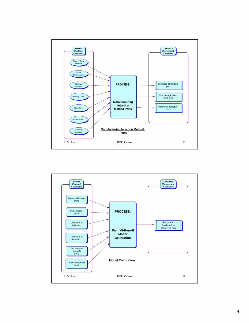
INPUTS(Factors)
X variables
OUTPUTS(Responses)Y variables
Type of Raw Material
Mold Temperature
PROCESS:
Manufacturing Injection
Molded Parts
p
Holding Pressure
Holding Time
Gate Size
thickness of molded part
% shrinkage from mold size
number of defective parts
L. M. Lye DOE Course 17
Screw Speed
Moisture Content
Manufacturing Injection Molded Parts
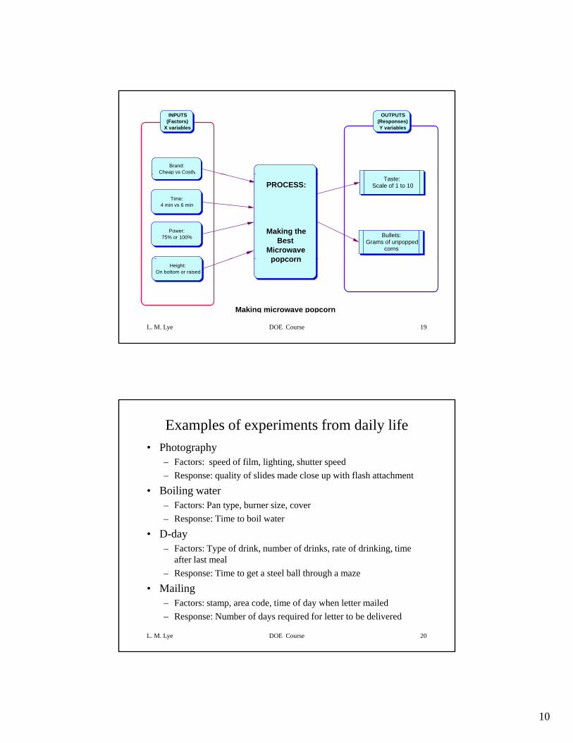
INPUTS(Factors)
X variables
OUTPUTS(Responses)Y variables
I iti l t
Impermeable layer (mm)
PROCESS:
Rainfall-Runoff Model
Calibration
Initial storage (mm)
Coefficient of Infiltration
Coefficient of Recession
R-square:Predicted vs
Observed Fits
L. M. Lye DOE Course 18
Soil Moisture Capacity
(mm)
Model CalibrationInitial Soil Moisture
(mm)
10
INPUTS(Factors)
X variables
OUTPUTS(Responses)Y variables
Brand:Cheap vs Costly
PROCESS:
Making the Best
Microwave popcorn
y
Time:4 min vs 6 min
Power:75% or 100%
Taste:Scale of 1 to 10
Bullets:Grams of unpopped
corns
L. M. Lye DOE Course 19
popcornHeight:
On bottom or raised
Making microwave popcorn
Examples of experiments from daily life• Photography
– Factors: speed of film, lighting, shutter speed– Response: quality of slides made close up with flash attachment
• Boiling water– Factors: Pan type, burner size, cover– Response: Time to boil water
• D-day– Factors: Type of drink, number of drinks, rate of drinking, time
after last meal
L. M. Lye DOE Course 20
– Response: Time to get a steel ball through a maze
• Mailing – Factors: stamp, area code, time of day when letter mailed– Response: Number of days required for letter to be delivered
11
More examples• Cooking
– Factors: amount of cooking wine, oyster sauce, sesame oil– Response: Taste of stewed chicken
• Sexual Pleasure– Factors: marijuana, screech, sauna– Response: Pleasure experienced in subsequent you know what
• Basketball– Factors: Distance from basket, type of shot, location on floor– Response: Number of shots made (out of 10) with basketball
L. M. Lye DOE Course 21
• Skiing– Factors: Ski type, temperature, type of wax– Response: Time to go down ski slope
Basic Principles
• Statistical design of experiments (DOE)g p ( )– the process of planning experiments so that
appropriate data can be analyzed by statistical methods that results in valid, objective, and meaningful conclusions from the data
– involves two aspects: design and statistical
L. M. Lye DOE Course 22
involves two aspects: design and statistical analysis
12
• Every experiment involves a sequence of activities:– Conjecture - hypothesis that motivates theConjecture - hypothesis that motivates the
experiment– Experiment - the test performed to investigate
the conjecture– Analysis - the statistical analysis of the data
from the experiment
L. M. Lye DOE Course 23
from the experiment– Conclusion - what has been learned about the
original conjecture from the experiment.
Three basic principles of Statistical DOE• Replication
– allows an estimate of experimental errorallows for a more precise estimate of the sample mean– allows for a more precise estimate of the sample mean value
• Randomization– cornerstone of all statistical methods– “average out” effects of extraneous factors– reduce bias and systematic errors
L. M. Lye DOE Course 24
reduce bias and systematic errors• Blocking
– increases precision of experiment– “factor out” variable not studied
13
Guidelines for Designing Experiments• Recognition of and statement of the problem
– need to develop all ideas about the objectives of theneed to develop all ideas about the objectives of the experiment - get input from everybody - use team approach.
• Choice of factors, levels, ranges, and response variables. – Need to use engineering judgment or prior test results.
L. M. Lye DOE Course 25
• Choice of experimental design– sample size, replicates, run order, randomization,
software to use, design of data collection forms.
• Performing the experiment– vital to monitor the process carefully. Easy to
underestimate logistical and planning aspects in a complex R and D environment.p
• Statistical analysis of data– provides objective conclusions - use simple graphics
whenever possible.
• Conclusion and recommendations– follow-up test runs and confirmation testing to validate
L. M. Lye DOE Course 26
p gthe conclusions from the experiment.
• Do we need to add or drop factors, change ranges, levels, new responses, etc.. ???
14
Using Statistical Techniques in Experimentation - things to keep in mind
• Use non-statistical knowledge of the problem– physical laws, background knowledgephysical laws, background knowledge
• Keep the design and analysis as simple as possible– Don’t use complex, sophisticated statistical techniques– If design is good, analysis is relatively straightforward– If design is bad - even the most complex and elegant
statistics cannot save the situation
L. M. Lye DOE Course 27
• Recognize the difference between practical and statistical significance– statistical significance ≠ practically significance
• Experiments are usually iterative– unwise to design a comprehensive experiment at the
start of the study– may need modification of factor levels, factors,
responses, etc.. - too early to know whether experiment would work
– use a sequential or iterative approach– should not invest more than 25% of resources in the
initial design
L. M. Lye DOE Course 28
initial design.– Use initial design as learning experiences to accomplish
the final objectives of the experiment.
15
DOE (II)
Factorial vs OFAT
L. M. Lye DOE Course 29
Factorial v.s. OFAT
• Factorial design - experimental trials or runs are performed at all possible combinations of factor levels in contrast to OFAT experiments.
• Factorial and fractional factorial experiments are among the most useful multi-factor experiments for engineering and scientific investigations.
L. M. Lye DOE Course 30
16
• The ability to gain competitive advantage requires extreme care in the design and conduct of
i t S i l tt ti t b id t j i texperiments. Special attention must be paid to joint effects and estimates of variability that are provided by factorial experiments.
• Full and fractional experiments can be conducted using a variety of statistical designs The design
L. M. Lye DOE Course 31
using a variety of statistical designs. The design selected can be chosen according to specific requirements and restrictions of the investigation.
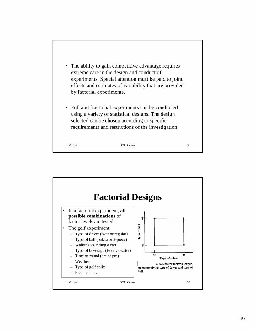
Factorial Designs• In a factorial experiment, all
ibl bi ti fpossible combinations of factor levels are tested
• The golf experiment:– Type of driver (over or regular)– Type of ball (balata or 3-piece)– Walking vs. riding a cart– Type of beverage (Beer vs water)
L. M. Lye DOE Course 32
yp g ( )– Time of round (am or pm)– Weather – Type of golf spike– Etc, etc, etc…
17
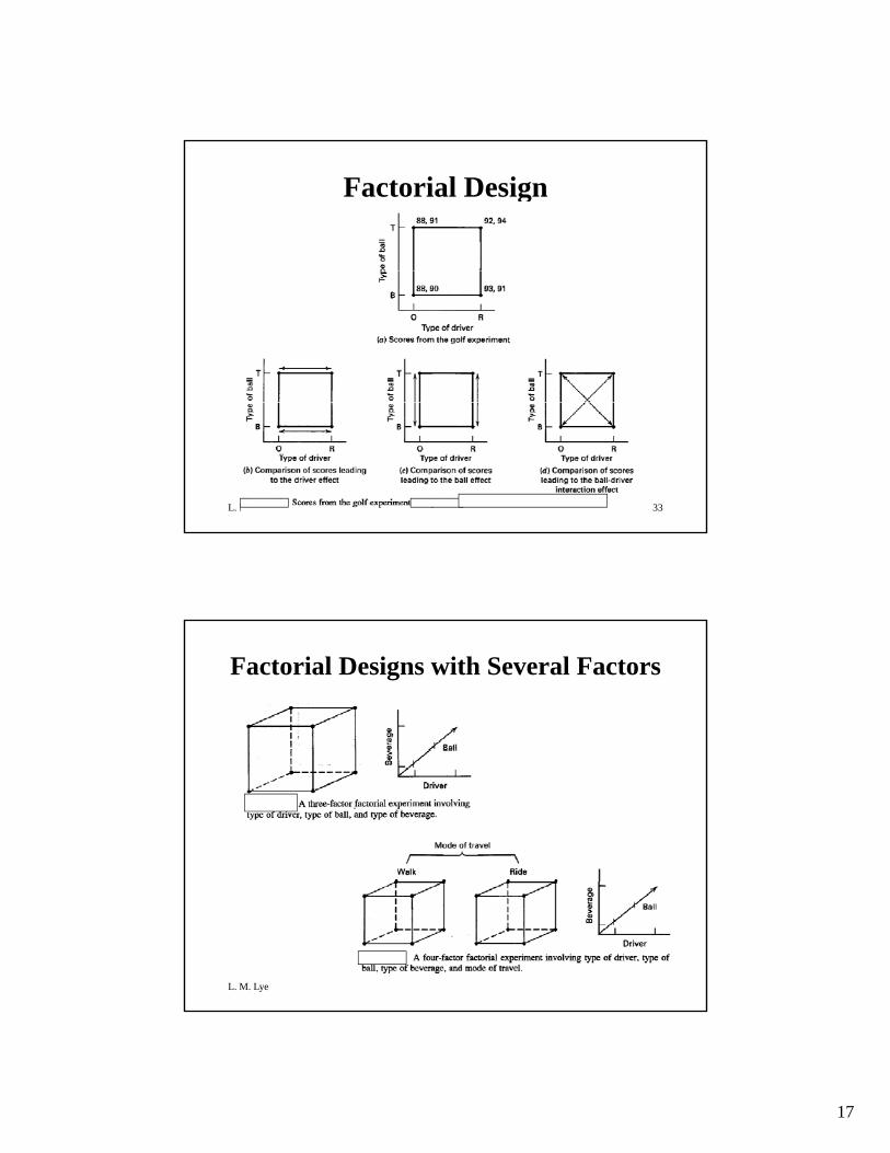
Factorial Design
L. M. Lye DOE Course 33
Factorial Designs with Several Factors
L. M. Lye DOE Course 34
18
Erroneous Impressions About Factorial Experiments
• Wasteful and do not compensate the extra effort with additional useful information - this folklore presumes that
k ( t ) th t f t i d d tlone knows (not assumes) that factors independently influence the responses (i.e. there are no factor interactions) and that each factor has a linear effect on the response - almost any reasonable type of experimentation will identify optimum levels of the factors
• Information on the factor effects becomes available only after the entire e periment is completed Takes too long
L. M. Lye DOE Course 35
after the entire experiment is completed. Takes too long. Actually, factorial experiments can be blocked and conducted sequentially so that data from each block can be analyzed as they are obtained.
One-factor-at-a-time experiments (OFAT)
• OFAT is a prevalent, but potentially disastrous type of experimentation commonly used by many engineers and scientists in both industry and academia.
• Tests are conducted by systematically changing the levels of one factor while holding the levels of all other factors fixed. The “optimal” level of the first factor is then selected.
• Subsequently, each factor in turn is varied and its
L. M. Lye DOE Course 36
“optimal” level selected while the other factors are held fixed.
19
One-factor-at-a-time experiments (OFAT)
• OFAT experiments are regarded as easier to implement, more easily understood, and more economical than f t i l i t B tt th t i l dfactorial experiments. Better than trial and error.
• OFAT experiments are believed to provide the optimum combinations of the factor levels.
• Unfortunately, each of these presumptions can generally be shown to be false except under very special circumstances.
• The key reasons why OFAT should not be conducted
L. M. Lye DOE Course 37
except under very special circumstances are:– Do not provide adequate information on interactions– Do not provide efficient estimates of the effects
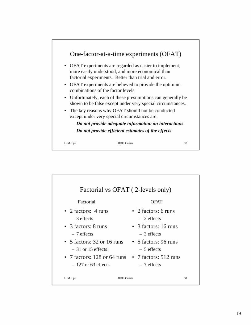
Factorial vs OFAT ( 2-levels only)
• 2 factors: 4 runs • 2 factors: 6 runsFactorial OFAT
• 2 factors: 4 runs– 3 effects
• 3 factors: 8 runs– 7 effects
• 5 factors: 32 or 16 runs31 15 ff t
• 2 factors: 6 runs– 2 effects
• 3 factors: 16 runs– 3 effects
• 5 factors: 96 runs5 ff t
L. M. Lye DOE Course 38
– 31 or 15 effects• 7 factors: 128 or 64 runs
– 127 or 63 effects
– 5 effects• 7 factors: 512 runs
– 7 effects
20
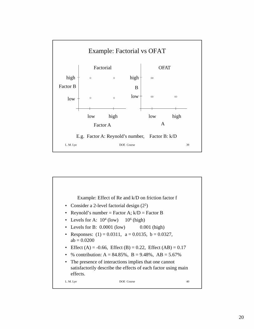
Example: Factorial vs OFAT
high high
OFATFactorial
l hi h
low
Factor B
high
B
high
low
l hi h
L. M. Lye DOE Course 39
Factor A
low high
E.g. Factor A: Reynold’s number, Factor B: k/D
low highA
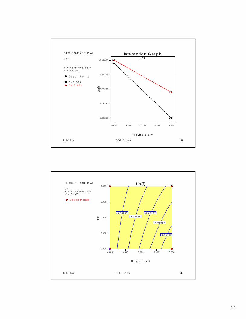
Example: Effect of Re and k/D on friction factor f• Consider a 2-level factorial design (22)• Reynold’s number = Factor A; k/D = Factor BReynold s number Factor A; k/D Factor B• Levels for A: 104 (low) 106 (high)• Levels for B: 0.0001 (low) 0.001 (high)• Responses: (1) = 0.0311, a = 0.0135, b = 0.0327,
ab = 0.0200• Effect (A) = -0.66, Effect (B) = 0.22, Effect (AB) = 0.17
L. M. Lye DOE Course 40
• % contribution: A = 84.85%, B = 9.48%, AB = 5.67%• The presence of interactions implies that one cannot
satisfactorily describe the effects of each factor using main effects.
21
D E S IG N -E A S E P l o t
L n (f )
X = A : R e y n o l d 's #Y = B : k/D
k /DInte ra c tio n G ra p h
- 3 64155
- 3.420382222
D e si g n P o i n ts
B - 0 .0 0 0B + 0 .0 0 1
Ln(f)
- 4 .08389
- 3.86272
3.64155
22
L. M. Lye DOE Course 41
R e yn o ld 's #
4.000 4.500 5.000 5.500 6.000
- 4.30507 22
D E S IG N -E A S E P l o t
L n (f )X = A : R e y n o l d 's #Y = B : k/D
D e si g n P o i n ts
L n(f)
0.0008
0.0010
k/D
0 .0003
0.0006
-4 . 1 5 7 6 2
-4 . 0 1 0 1 7
-3 . 8 6 2 7 2-3 . 7 1 5 2 8
-3 . 5 6 7 8 3
L. M. Lye DOE Course 42
R e yn o ld 's #
4.000 4.500 5.000 5.500 6.000
0.0001
22
D E S IG N -E A S E P l o t
L n (f )X = A : R e y n o l d 's #Y = B : k/D
-3 8 6 2 7 2
-3 . 6 4 1 5 5
-3 . 4 2 0 3 8
-4 . 3 0 5 0 7
-4 . 0 8 3 8 9
-3 . 8 6 2 7 2
Ln(
f)
0 . 0 0 0 8
0 . 0 0 1 0
L. M. Lye DOE Course 43
4 . 0 0 0 4 . 5 0 0
5 . 0 0 0 5 . 5 0 0
6 . 0 0 0
0 . 0 0 0 1
0 . 0 0 0 3
0 . 0 0 0 6
R e y n o l d 's #
k/D
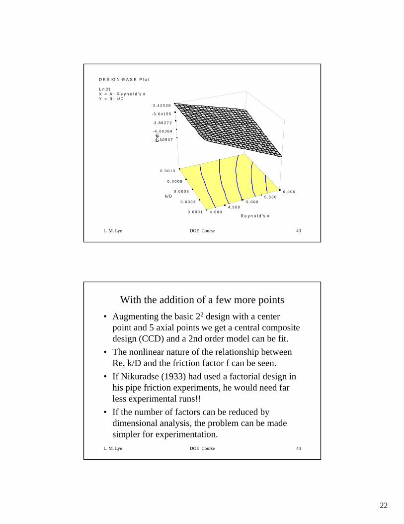
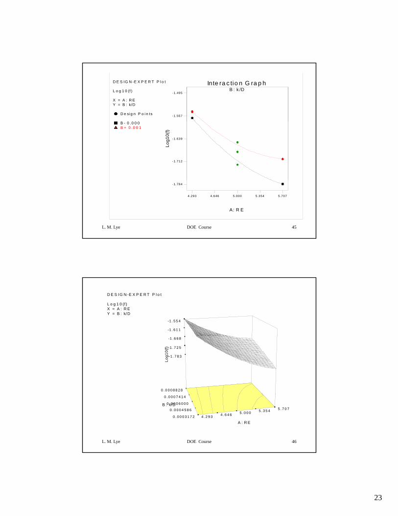
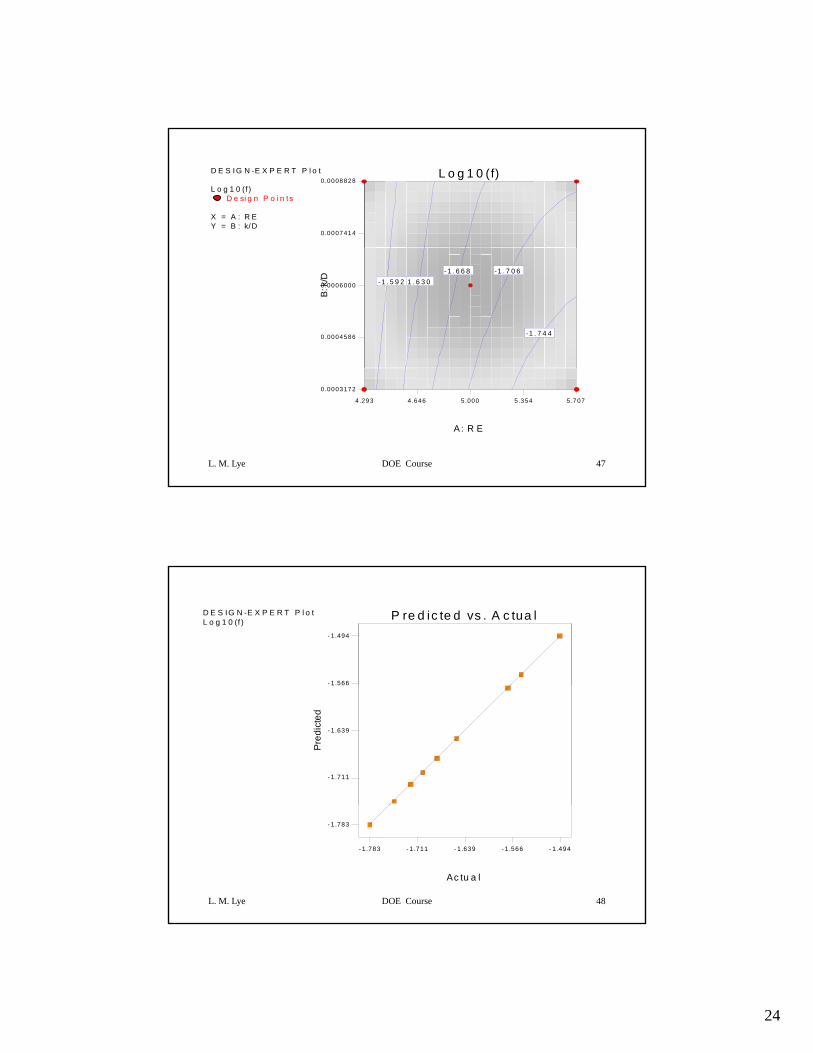
With the addition of a few more points• Augmenting the basic 22 design with a center
point and 5 axial points we get a central composite design (CCD) and a 2nd order model can be fit.design (CCD) and a 2nd order model can be fit.
• The nonlinear nature of the relationship between Re, k/D and the friction factor f can be seen.
• If Nikuradse (1933) had used a factorial design in his pipe friction experiments, he would need far less experimental runs!!
L. M. Lye DOE Course 44
less experimental runs!! • If the number of factors can be reduced by
dimensional analysis, the problem can be made simpler for experimentation.
23
D E S IG N -E X P E R T P l o t
L o g 1 0 (f )
X = A : R EY = B : k/D
D e si g n P o i n ts
B : k /DInte ra c tio n G ra p h
- 1.567
- 1.495
B - 0 .0 0 0B + 0 .0 0 1
Log1
0(f)
- 1 .712
- 1.639
L. M. Lye DOE Course 45
A: R E
4.293 4.646 5.000 5.354 5.707
- 1.784
D E S IG N -E X P E R T P l o t
L o g 1 0 (f )X = A : R EY = B : k/D
-1 . 6 1 1
-1 . 5 5 4
-1 . 7 8 3
-1 . 7 2 5
-1 . 6 6 8
Log
10(f)
0 . 0 0 0 8 8 2 8
L. M. Lye DOE Course 46
4 . 2 9 3 4 . 6 4 6 5 . 0 0 0 5 . 3 5 4 5 . 7 0 7
0 . 0 0 0 3 1 7 2
0 . 0 0 0 4 5 8 6
0 . 0 0 0 6 0 0 0
0 . 0 0 0 7 4 1 4
A : R E
B : k/D
24
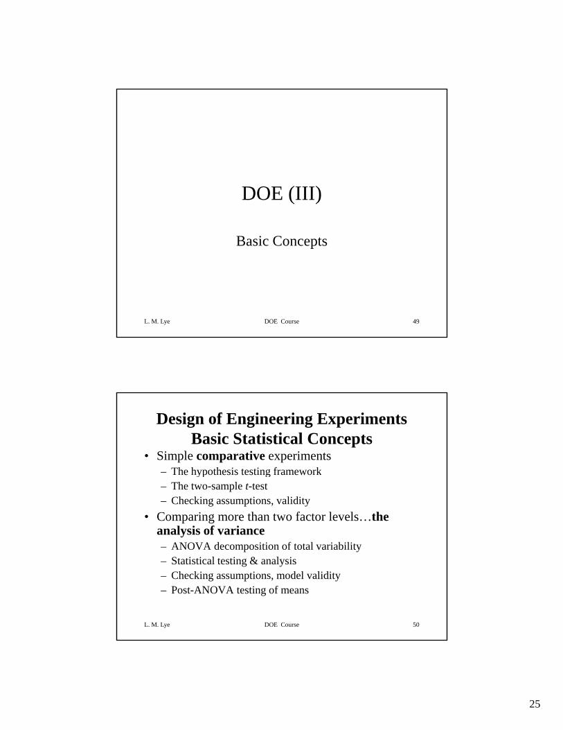
D E S IG N -E X P E R T P l o t
L o g 1 0 (f )D e si g n P o i n t s
X = A : R EY = B : k/D
L o g 1 0 (f)
0.0007414
0 .0008828
B: k
/D0 .0004586
0 .0006000
-1 . 7 4 4
-1 . 7 0 6-1 . 6 6 8-1 . 6 3 0-1 . 5 9 2
L. M. Lye DOE Course 47
A: R E
4.293 4.646 5.000 5.354 5.707
0 .0003172
D E S IG N -E X P E R T P l o tL o g 1 0 (f ) P re d ic te d vs . A c tua l
- 1.566
- 1.494
Pred
icte
d
- 1 .711
- 1.639
1.566
L. M. Lye DOE Course 48
Ac tu a l
- 1.783
- 1.783 - 1.711 - 1.639 - 1.566 - 1.494
25
DOE (III)
Basic Concepts
L. M. Lye DOE Course 49
Design of Engineering ExperimentsBasic Statistical Concepts
• Simple comparative experiments– The hypothesis testing frameworke ypot es s test g a ewo– The two-sample t-test– Checking assumptions, validity
• Comparing more than two factor levels…theanalysis of variance– ANOVA decomposition of total variability
St ti ti l t ti & l i
L. M. Lye DOE Course 50
– Statistical testing & analysis– Checking assumptions, model validity– Post-ANOVA testing of means
26
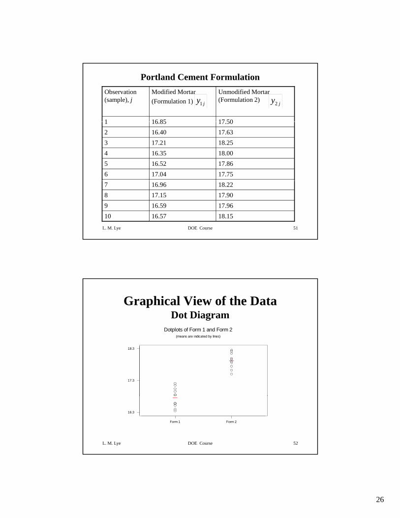
Portland Cement Formulation
17 5016 851
Unmodified Mortar (Formulation 2)
Modified Mortar(Formulation 1)
Observation (sample), j
1 jy 2 jy
17.7517.04617.8616.52518.0016.35418.2517.21317.6316.40217.5016.851
L. M. Lye DOE Course 51
18.1516.571017.9616.59917.9017.15818.2216.967
Graphical View of the DataDot Diagram
Dotplots of Form 1 and Form 2(means are indicated by lines)
17.3
18.3
(means are indicated by lines)
L. M. Lye DOE Course 52
Form 1 Form 2
16.3
27
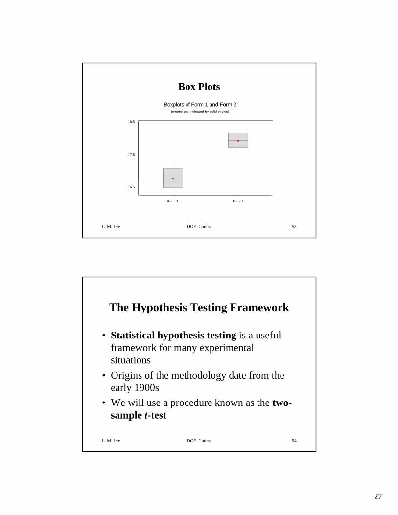
Box Plots
18 5
Boxplots of Form 1 and Form 2(means are indicated by solid circles)
17.5
18.5
L. M. Lye DOE Course 53
Form 1 Form 2
16.5
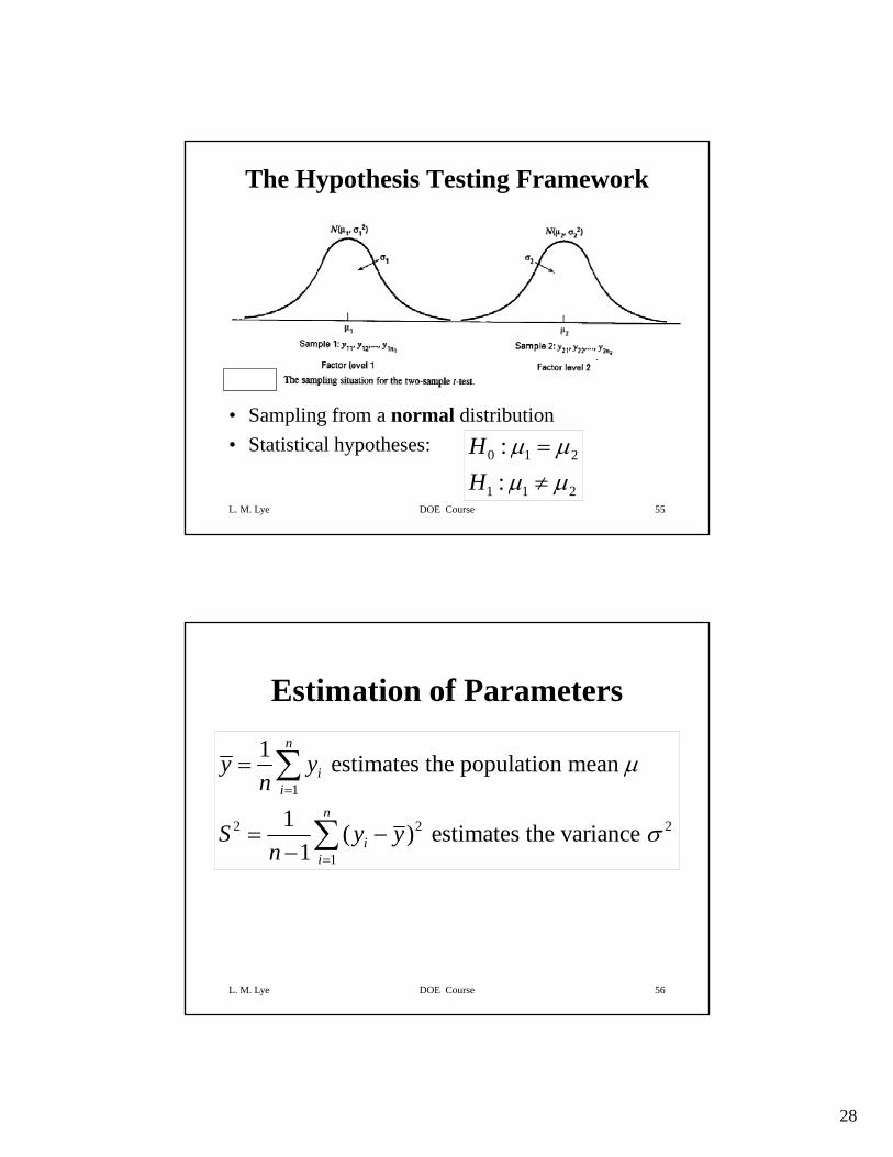
The Hypothesis Testing Framework
• Statistical hypothesis testing is a useful• Statistical hypothesis testing is a useful framework for many experimental situations
• Origins of the methodology date from the early 1900s
L. M. Lye DOE Course 54
• We will use a procedure known as the two-sample t-test
28
The Hypothesis Testing Framework
L. M. Lye DOE Course 55
• Sampling from a normal distribution• Statistical hypotheses: 0 1 2
1 1 2
::
HH
μ μμ μ
=≠
Estimation of Parameters
1 n
∑1
2 2 2
1
1 estimates the population mean
1 ( ) estimates the variance 1
ii
n
ii
y yn
S y yn
μ
σ
=
=
=
= −−
∑
∑
L. M. Lye DOE Course 56
29
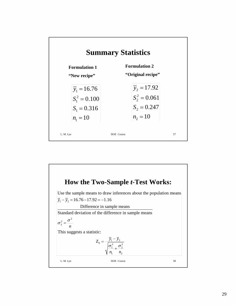
Summary Statistics
Formulation 1 Formulation 2
12
1
16.76
0.1000 316
y
SS
=
=
222
17.92
0.0610 247
y
SS
=
=
“New recipe” “Original recipe”
L. M. Lye DOE Course 57
1
1
0.31610
Sn==
2
2
0.24710
Sn
==
How the Two-Sample t-Test Works:Use the sample means to draw inferences about the population means
16 76 17 92 1 161 2
22y
16.76 17.92 1.16Difference in sample means
Standard deviation of the difference in sample means
This suggests a statistic:
y y
nσσ
− = − = −
=
L. M. Lye DOE Course 58
This suggests a statistic:
1 20 2 2
1 2
1 2
Z y y
n nσ σ−
=
+
30
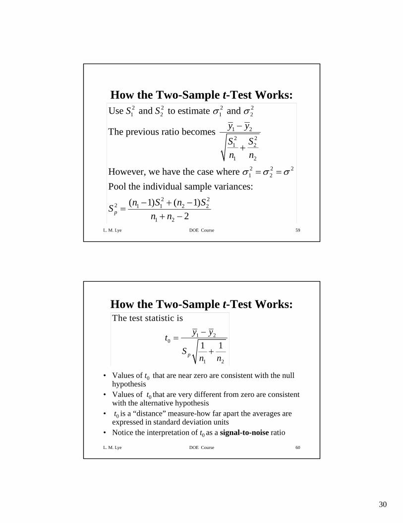
How the Two-Sample t-Test Works:2 2 2 2
1 2 1 2Use and to estimate and S S σ σ
1 22 2
1 2
1 2
2 2 21 2
The previous ratio becomes
However, we have the case where
y yS Sn n
σ σ σ
−
+
= =
L. M. Lye DOE Course 59
2 22 1 1 2 2
1 2
Pool the individual sample variances:( 1) ( 1)
2pn S n SS
n n− + −
=+ −
How the Two-Sample t-Test Works:
1 20
The test statistic isy yt −
=
• Values of t0 that are near zero are consistent with the null hypothesis
• Values of t0 that are very different from zero are consistent
0
1 2
1 1
p
tS
n n+
L. M. Lye DOE Course 60
with the alternative hypothesis• t0 is a “distance” measure-how far apart the averages are
expressed in standard deviation units• Notice the interpretation of t0 as a signal-to-noise ratio
31
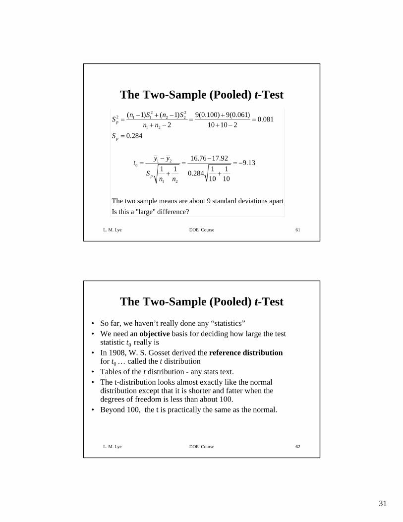
The Two-Sample (Pooled) t-Test2 2
2 1 1 2 2( 1) ( 1) 9(0.100) 9(0.061) 0.0812 10 10 2p
n S n SS − + − += = =
1 2
1 20
1 2
2 10 10 20.284
16.76 17.92 9.131 1 1 10.284
10 10
p
p
p
n nS
y ytS
n n
+ − + −=
− −= = = −
+ +
L. M. Lye DOE Course 61
1 2
The two sample means are about 9 standard deviations apartIs this a "large" difference?
The Two-Sample (Pooled) t-Test
• So far, we haven’t really done any “statistics”• We need an objective basis for deciding how large the test
i i ll istatistic t0 really is• In 1908, W. S. Gosset derived the reference distribution
for t0 … called the t distribution• Tables of the t distribution - any stats text.• The t-distribution looks almost exactly like the normal
distribution except that it is shorter and fatter when the degrees of freedom is less than about 100
L. M. Lye DOE Course 62
degrees of freedom is less than about 100. • Beyond 100, the t is practically the same as the normal.
32
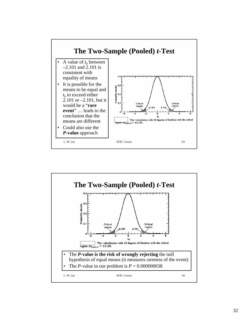
The Two-Sample (Pooled) t-Test• A value of t0 between
–2.101 and 2.101 is consistent with equality of means
• It is possible for the means to be equal and t0 to exceed either 2.101 or –2.101, but it would be a “rareevent” … leads to the
L. M. Lye DOE Course 63
conclusion that the means are different
• Could also use the P-value approach
The Two-Sample (Pooled) t-Test
L. M. Lye DOE Course 64
• The P-value is the risk of wrongly rejecting the null hypothesis of equal means (it measures rareness of the event)
• The P-value in our problem is P = 0.000000038
33
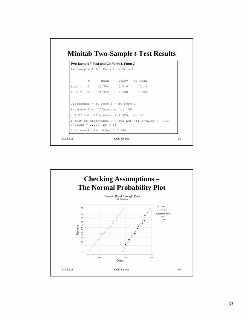
Minitab Two-Sample t-Test ResultsTwo-Sample T-Test and CI: Form 1, Form 2Two-sample T for Form 1 vs Form 2
N Mean StDev SE Mean
Form 1 10 16.764 0.316 0.10
Form 2 10 17.922 0.248 0.078
Difference = mu Form 1 - mu Form 2
Estimate for difference: -1 158
L. M. Lye DOE Course 65
Estimate for difference: 1.158
95% CI for difference: (-1.425, -0.891)
T-Test of difference = 0 (vs not =): T-Value = -9.11 P-Value = 0.000 DF = 18
Both use Pooled StDev = 0.284
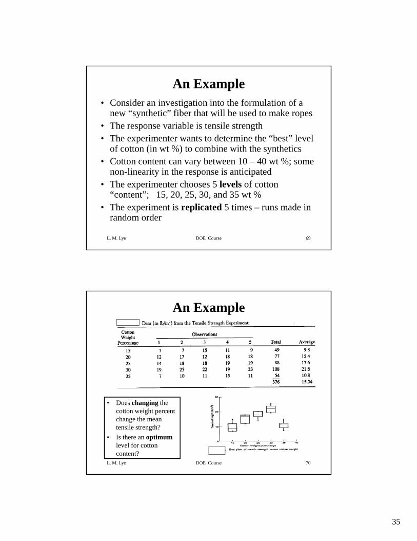
Checking Assumptions –The Normal Probability Plot
Tension Bond Strength DataML Estimates
Form 1
Form 2
20304050607080
90
95
99
Per
cent
AD*
1.2091.387
Goodness of Fit
L. M. Lye DOE Course 66
16.5 17.5 18.5
1
5
10
Data

34
Importance of the t-Test
• Provides an objective framework for simple• Provides an objective framework for simple comparative experiments
• Could be used to test all relevant hypotheses in a two-level factorial design, because all of these hypotheses involve the mean
L. M. Lye DOE Course 67
response at one “side” of the cube versus the mean response at the opposite “side” of the cube
What If There Are More Than Two Factor Levels?
• The t-test does not directly applyTh l t f ti l it ti h th ith• There are lots of practical situations where there are either more than two levels of interest, or there are several factors of simultaneous interest
• The analysis of variance (ANOVA) is the appropriate analysis “engine” for these types of experiments
• The ANOVA was developed by Fisher in the early 1920s, and
L. M. Lye DOE Course 68
initially applied to agricultural experiments• Used extensively today for industrial experiments
35
An Example• Consider an investigation into the formulation of a
new “synthetic” fiber that will be used to make ropes• The response variable is tensile strengthThe response variable is tensile strength• The experimenter wants to determine the “best” level
of cotton (in wt %) to combine with the synthetics• Cotton content can vary between 10 – 40 wt %; some
non-linearity in the response is anticipated• The experimenter chooses 5 levels of cotton
L. M. Lye DOE Course 69
p“content”; 15, 20, 25, 30, and 35 wt %
• The experiment is replicated 5 times – runs made in random order
An Example
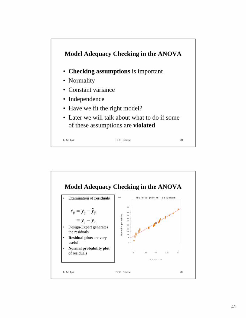
• Does changing the cotton weight percent
L. M. Lye DOE Course 70
g pchange the mean tensile strength?
• Is there an optimumlevel for cotton content?
36
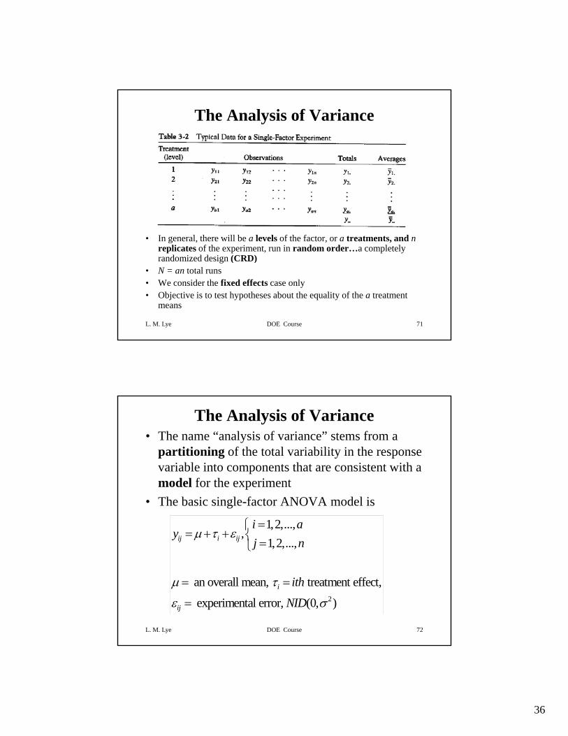
The Analysis of Variance
• In general, there will be a levels of the factor, or a treatments, and nreplicates of the experiment, run in random order…a completely
d i d d i (CRD)
L. M. Lye DOE Course 71
randomized design (CRD)• N = an total runs• We consider the fixed effects case only• Objective is to test hypotheses about the equality of the a treatment
means
The Analysis of Variance• The name “analysis of variance” stems from a
partitioning of the total variability in the response variable into components that are consistent with a
d l f h imodel for the experiment• The basic single-factor ANOVA model is
1,2,...,,
1,2,...,ij i ij
i ay
j nμ τ ε
=⎧= + + ⎨ =⎩
L. M. Lye DOE Course 72
2
an overall mean, treatment effect,
experimental error, (0, )i
ij
ith
NID
μ τ
ε σ
= =
=
37
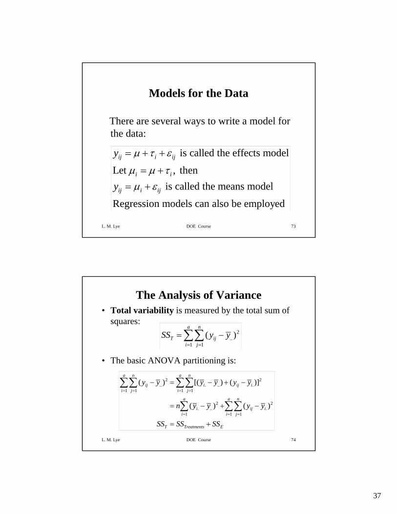
Models for the Data
There are several ways to write a model forThere are several ways to write a model for the data:
is called the effects model
Let , then ij i ij
i i
y μ τ ε
μ μ τ
= + +
= +
L. M. Lye DOE Course 73
is called the means model
Regression models can also be employedij i ijy μ ε= +
The Analysis of Variance• Total variability is measured by the total sum of
squares:2( )
a n
SS y y=∑∑
• The basic ANOVA partitioning is:
..1 1
( )T iji j
SS y y= =
= −∑∑
2 2.. . .. .
1 1 1 1( ) [( ) ( )]
a n a n
ij i ij ii j i j
y y y y y y= = = =
− = − + −∑∑ ∑∑
L. M. Lye DOE Course 74
2 2. .. .
1 1 1
( ) ( )
j j
a a n
i ij ii i j
T Treatments E
n y y y y
SS SS SS= = =
= − + −
= +
∑ ∑∑
38
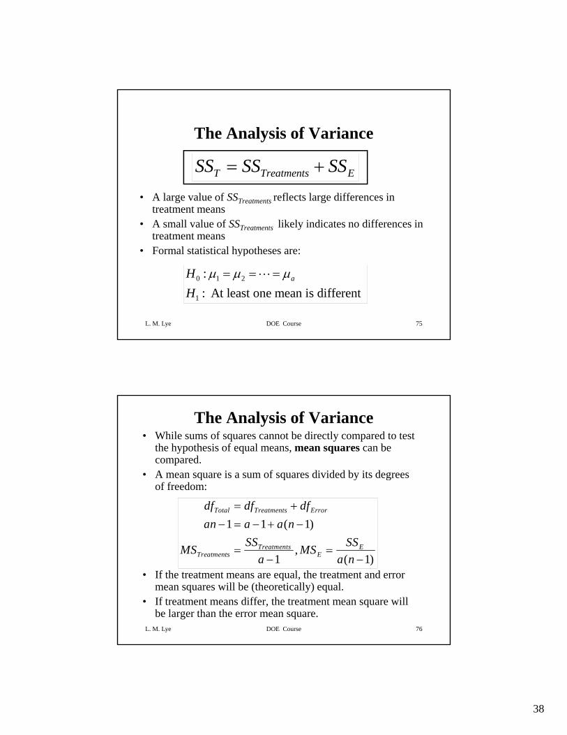
The Analysis of Variance
T Treatments ESS SS SS= +
• A large value of SSTreatments reflects large differences in treatment means
• A small value of SSTreatments likely indicates no differences in treatment means
• Formal statistical hypotheses are:
T Treatments E
L. M. Lye DOE Course 75
yp
0 1 2
1
:: At least one mean is different
aHH
μ μ μ= = =L
The Analysis of Variance• While sums of squares cannot be directly compared to test
the hypothesis of equal means, mean squares can be compared.
• A mean square is a sum of squares divided by its degrees q q y gof freedom:
1 1 ( 1)
,1 ( 1)
Total Treatments Error
Treatments ETreatments E
df df dfan a a n
SS SSMS MSa a n
= +− = − + −
= =− −
L. M. Lye DOE Course 76
• If the treatment means are equal, the treatment and error mean squares will be (theoretically) equal.
• If treatment means differ, the treatment mean square will be larger than the error mean square.
1 ( 1)a a n
39
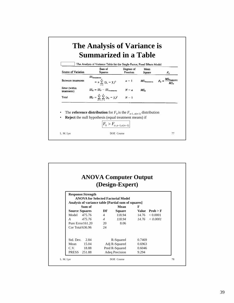
The Analysis of Variance is Summarized in a Table
L. M. Lye DOE Course 77
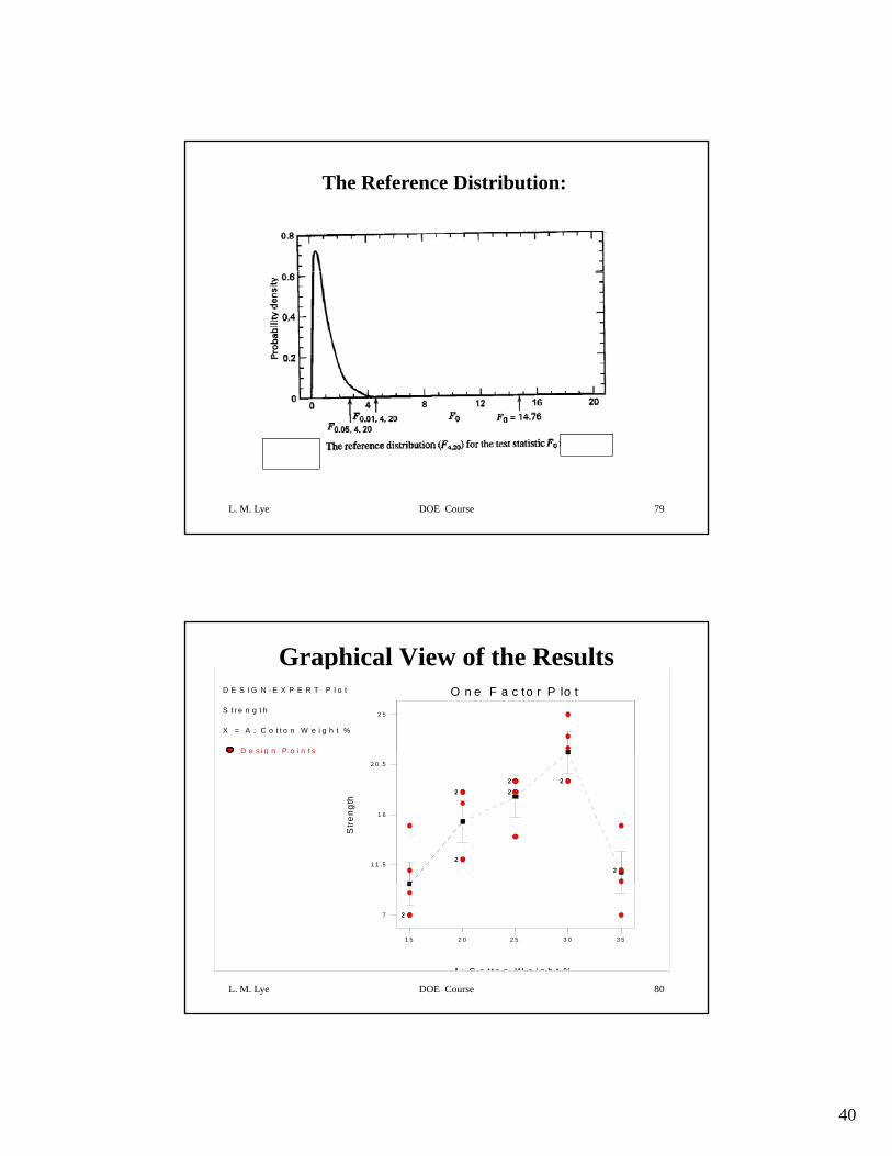
• The reference distribution for F0 is the Fa-1, a(n-1) distribution• Reject the null hypothesis (equal treatment means) if
0 , 1, ( 1)a a nF Fα − −>
ANOVA Computer Output (Design-Expert)
Response:StrengthANOVA for Selected Factorial Model
Analysis of variance table [Partial sum of squares]Sum of Mean F
Source Squares DF Square Value Prob > FModel 475.76 4 118.94 14.76 < 0.0001A 475.76 4 118.94 14.76 < 0.0001Pure Error161.20 20 8.06Cor Total 636.96 24
L. M. Lye DOE Course 78
Std. Dev. 2.84 R-Squared 0.7469Mean 15.04 Adj R-Squared 0.6963C.V. 18.88 Pred R-Squared 0.6046PRESS 251.88 Adeq Precision 9.294
40
The Reference Distribution:
L. M. Lye DOE Course 79
Graphical View of the ResultsD E S I G N - E X P E R T P l o t
S t re n g t h X = A : C o t t o n W e i g h t %
D e s i g n P o i n t s
O n e F a c to r P lo t
2 5
D e s i g n P o i n t s
Stre
ngth
1 1 .5
1 6
2 0 .5
22
22 22
22 22
22
L. M. Lye DOE Course 80
A : C o t to n W e i g h t %
1 5 2 0 2 5 3 0 3 5
7 22
41
Model Adequacy Checking in the ANOVA
• Checking assumptions is important• Normality• Constant variance• Independence• Have we fit the right model?
L. M. Lye DOE Course 81
g• Later we will talk about what to do if some
of these assumptions are violated
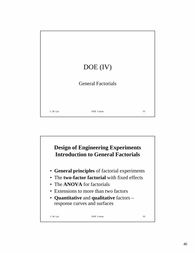
Model Adequacy Checking in the ANOVA
• Examination of residuals l o t N o rm a l p lo t o f re s i d u a ls
9 9
• Design-Expert generates the residuals
• Residual plots are very useful
.
ˆij ij ij
ij i
e y y
y y
= −
= −
Nor
mal
% p
roba
bilit
y
1
5
1 0
2 0
3 0
5 0
7 0
8 0
9 0
9 5
9 9
L. M. Lye DOE Course 82
useful• Normal probability plot
of residualsR e s i d u a l
- 3 .8 - 1 .5 5 0 .7 2 .9 5 5 .2
1
42
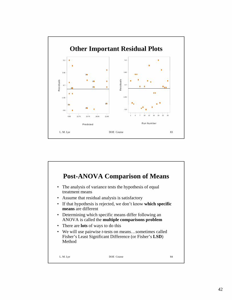
Other Important Residual Plots5.2 5.2
22
22
22
22
22
22
Res
idua
ls
-1.55
0.7
2.95
Res
idua
ls
-1.55
0.7
2.95
L. M. Lye DOE Course 83
22
22
Predicted
-3.8
9.80 12.75 15.70 18.65 21.60
Run Num ber
-3.8
1 4 7 10 13 16 19 22 25
Post-ANOVA Comparison of Means• The analysis of variance tests the hypothesis of equal
treatment means• Assume that residual analysis is satisfactory• If that hypothesis is rejected, we don’t know which specific
means are different • Determining which specific means differ following an
ANOVA is called the multiple comparisons problem• There are lots of ways to do this
L. M. Lye DOE Course 84
• We will use pairwise t-tests on means…sometimes called Fisher’s Least Significant Difference (or Fisher’s LSD) Method
43
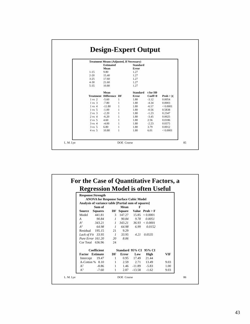
Design-Expert OutputTreatment Means (Adjusted, If Necessary)
Estimated StandardMean Error
1-15 9.80 1.272-20 15.40 1.272 20 15.40 1.273-25 17.60 1.274-30 21.60 1.275-35 10.80 1.27
Mean Standard t for H0Treatment Difference DF Error Coeff=0 Prob > |t|1 vs 2 -5.60 1 1.80 -3.12 0.00541 vs 3 -7.80 1 1.80 -4.34 0.00031 vs 4 -11.80 1 1.80 -6.57 < 0.00011 vs 5 -1.00 1 1.80 -0.56 0.58382 vs 3 2 20 1 1 80 1 23 0 2347
L. M. Lye DOE Course 85
2 vs 3 -2.20 1 1.80 -1.23 0.23472 vs 4 -6.20 1 1.80 -3.45 0.00252 vs 5 4.60 1 1.80 2.56 0.01863 vs 4 -4.00 1 1.80 -2.23 0.03753 vs 5 6.80 1 1.80 3.79 0.00124 vs 5 10.80 1 1.80 6.01 < 0.0001
For the Case of Quantitative Factors, a Regression Model is often UsefulResponse:Strength
ANOVA for Response Surface Cubic ModelAnalysis of variance table [Partial sum of squares]
Sum of Mean FSource Squares DF Square Value Prob > FSource Squares DF Square Value Prob > FModel 441.81 3 147.27 15.85 < 0.0001A 90.84 1 90.84 9.78 0.0051A2 343.21 1 343.21 36.93 < 0.0001A3 64.98 1 64.98 6.99 0.0152Residual 195.15 21 9.29Lack of Fit 33.95 1 33.95 4.21 0.0535Pure Error 161.20 20 8.06Cor Total 636.96 24
L. M. Lye DOE Course 86
Coefficient Standard 95% CI 95% CIFactor Estimate DF Error Low High VIFIntercept 19.47 1 0.95 17.49 21.44A-Cotton % 8.10 1 2.59 2.71 13.49 9.03A2 -8.86 1 1.46 -11.89 -5.83 1.00A3 -7.60 1 2.87 -13.58 -1.62 9.03
44
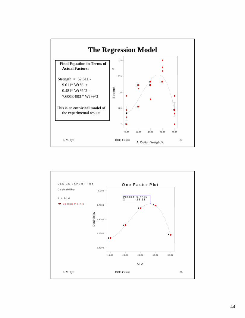
The Regression Model
Final Equation in Terms of Actual Factors: %
25
Strength = 62.611 -9.011* Wt % + 0.481* Wt %^2 -7.600E-003 * Wt %^3
This is an empirical model of 11.5
16
20.5
Stre
ngth
22
22 22
22 22
22
L. M. Lye DOE Course 87
the experimental results
15.00 20.00 25.00 30.00 35.00
7
A: Cotton Weight %
22
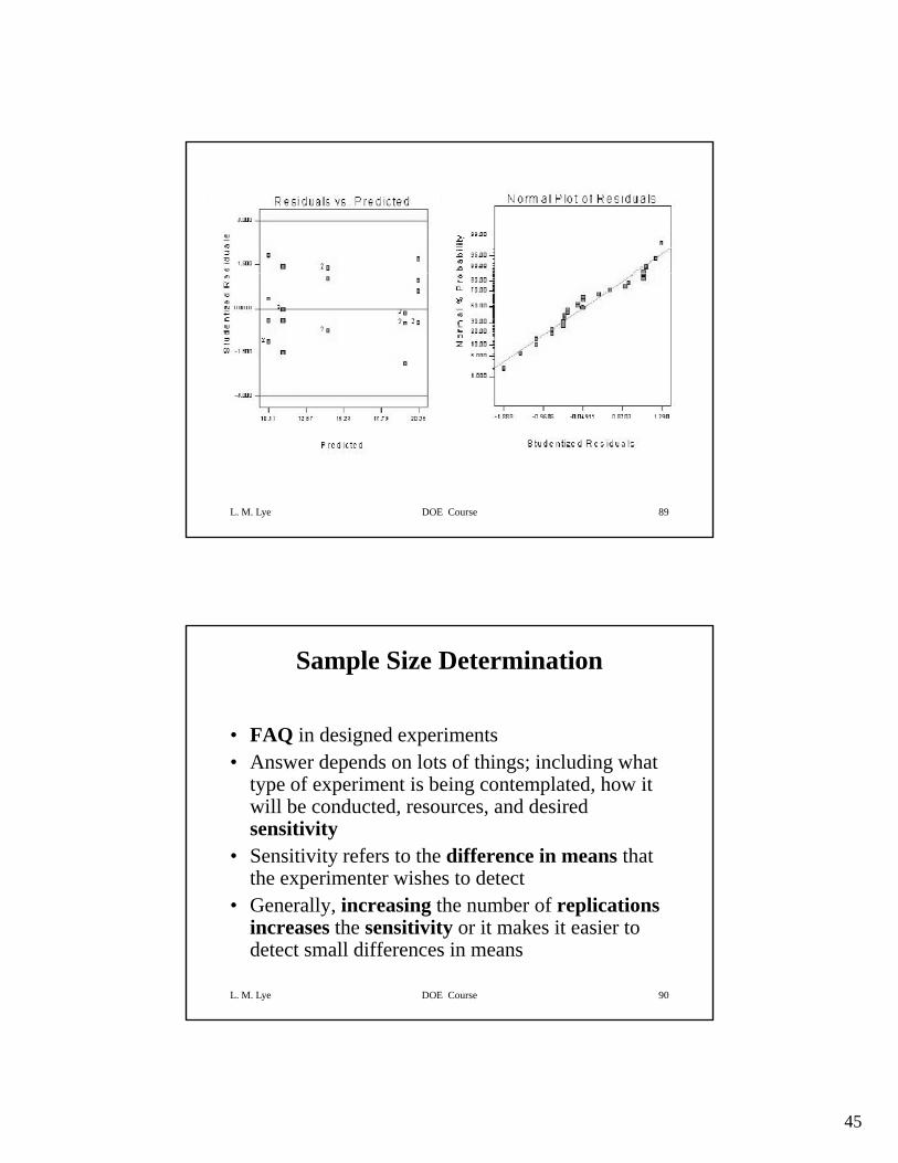
D E S I G N -E X P E R T P l o t
D e si ra b i l i t y
X = A : A
D e si g n P o i n t s 0 .7 50 0
1 .0 00
O n e F a c to r P lo t
55555
Pr e d ic t 0 .7 7 2 5X 2 8 .2 3
0.2 50 0
0 .5 00 0
Des
irabi
lity
66
66666
55555
55555
66666
L. M. Lye DOE Course 88
15 .00 2 0 .0 0 25 .0 0 30 .00 3 5 .0 0
0 .0 00 0
A : A
45
L. M. Lye DOE Course 89
Sample Size Determination
• FAQ in designed experimentsA d d l t f thi i l di h t• Answer depends on lots of things; including what type of experiment is being contemplated, how it will be conducted, resources, and desired sensitivity
• Sensitivity refers to the difference in means that the experimenter wishes to detect
L. M. Lye DOE Course 90
p• Generally, increasing the number of replications
increases the sensitivity or it makes it easier to detect small differences in means
46
DOE (IV)
General Factorials
L. M. Lye DOE Course 91
Design of Engineering ExperimentsIntroduction to General Factorials
• General principles of factorial experiments• The two-factor factorial with fixed effects• The ANOVA for factorials• Extensions to more than two factors
L. M. Lye DOE Course 92
• Quantitative and qualitative factors –response curves and surfaces
47
Some Basic Definitions
Definition of a factor effect: The change in the mean response when the factor is changed from low to high
40 52 20 30+ +
L. M. Lye DOE Course 93
40 52 20 30 212 2
30 52 20 40 112 2
52 20 30 40 12 2
A A
B B
A y y
B y y
AB
+ −
+ −
+ += − = − =
+ += − = − =
+ += − = −
The Case of Interaction:
50 12 20 40 12 2A A
A y y+ −
+ += − = − =
L. M. Lye DOE Course 94
2 240 12 20 50 9
2 212 20 40 50 29
2 2
A A
B BB y y
AB
+ −
+ += − = − = −
+ += − = −
48
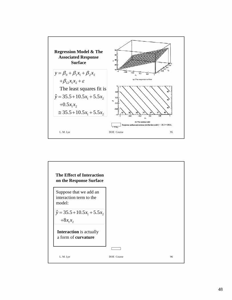
Regression Model & The Associated Response
Surface
0 1 1 2 2
12 1 2
1 2
The least squares fit isˆ 35.5 10.5 5.5
0 5
y x xx x
y x xx x
β β ββ ε
= + ++ +
= + ++
L. M. Lye DOE Course 95
1 2
1 2
0.535.5 10.5 5.5
x xx x
+≅ + +
The Effect of Interaction on the Response Surface
Suppose that we add an interaction term to the model:
1 2
1 2
ˆ 35.5 10.5 5.58
y x xx x
= + ++
L. M. Lye DOE Course 96
Interaction is actually a form of curvature
49
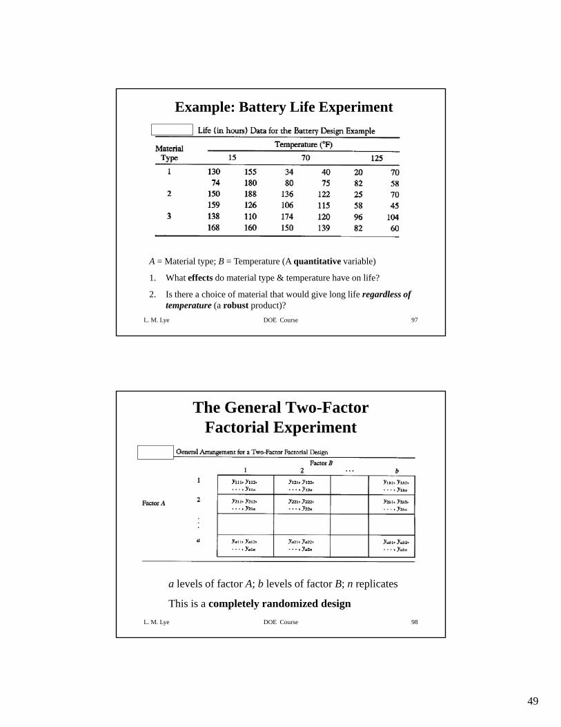
Example: Battery Life Experiment
L. M. Lye DOE Course 97
A = Material type; B = Temperature (A quantitative variable)
1. What effects do material type & temperature have on life?
2. Is there a choice of material that would give long life regardless of temperature (a robust product)?
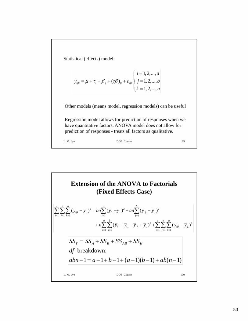
The General Two-Factor Factorial Experiment
L. M. Lye DOE Course 98
a levels of factor A; b levels of factor B; n replicates
This is a completely randomized design
50
Statistical (effects) model:
1, 2,...,i a=⎧⎪
, , ,( ) 1,2,...,
1, 2,...,ijk i j ij ijky j b
k nμ τ β τβ ε
⎧⎪= + + + + =⎨⎪ =⎩
Other models (means model, regression models) can be useful
L. M. Lye DOE Course 99
Regression model allows for prediction of responses when we have quantitative factors. ANOVA model does not allow for prediction of responses - treats all factors as qualitative.
Extension of the ANOVA to Factorials (Fixed Effects Case)
2 2 2( ) ( ) ( )a b n a b
b∑∑∑ ∑ ∑2 2 2... .. ... . . ...
1 1 1 1 1
2 2. .. . . ... .
1 1 1 1 1
( ) ( ) ( )
( ) ( )
ijk i ji j k i j
a b a b n
ij i j ijk iji j i j k
y y bn y y an y y
n y y y y y y
= = = = =
= = = = =
− = − + −
+ − − + + −
∑∑∑ ∑ ∑
∑∑ ∑∑∑
T A B AB ESS SS SS SS SS= + + +
L. M. Lye DOE Course 100
breakdown:1 1 1 ( 1)( 1) ( 1)
dfabn a b a b ab n− = − + − + − − + −
51
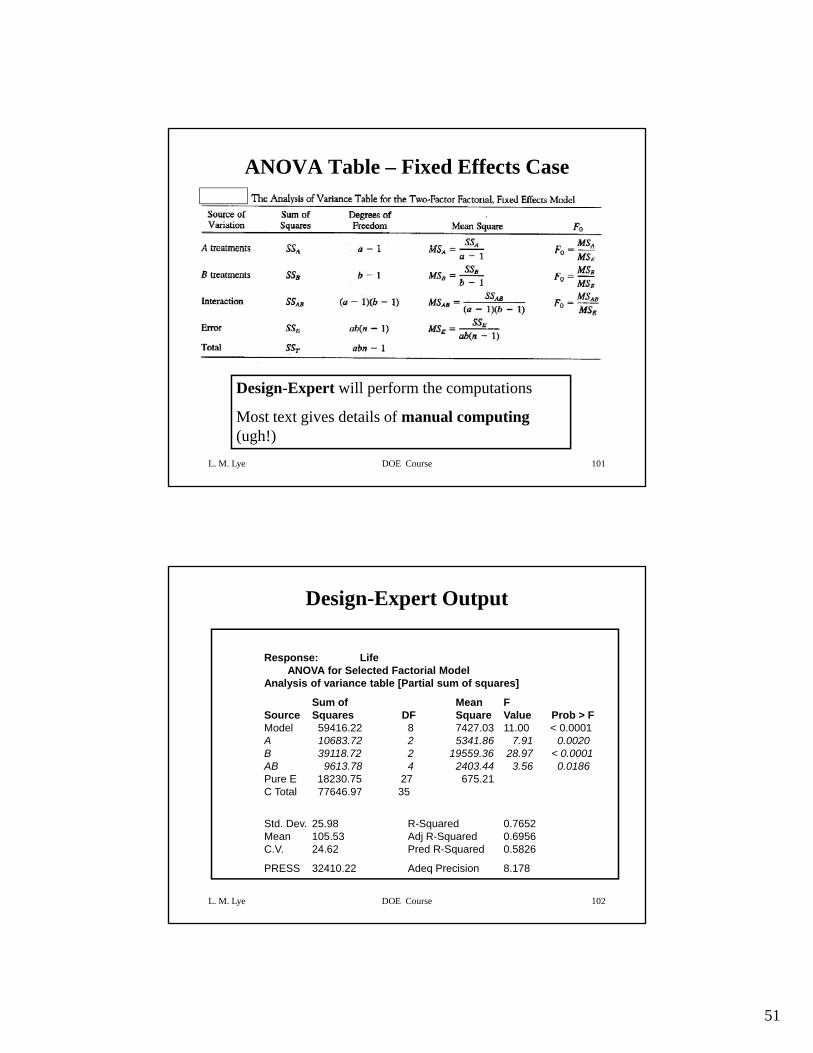
ANOVA Table – Fixed Effects Case
L. M. Lye DOE Course 101
Design-Expert will perform the computations
Most text gives details of manual computing(ugh!)
Design-Expert Output
Response: LifeANOVA for Selected Factorial Model
Analysis of variance table [Partial sum of squares]Analysis of variance table [Partial sum of squares]
Sum of Mean FSource Squares DF Square Value Prob > FModel 59416.22 8 7427.03 11.00 < 0.0001A 10683.72 2 5341.86 7.91 0.0020B 39118.72 2 19559.36 28.97 < 0.0001AB 9613.78 4 2403.44 3.56 0.0186Pure E 18230.75 27 675.21C Total 77646.97 35
L. M. Lye DOE Course 102
Std. Dev. 25.98 R-Squared 0.7652Mean 105.53 Adj R-Squared 0.6956C.V. 24.62 Pred R-Squared 0.5826
PRESS 32410.22 Adeq Precision 8.178
52
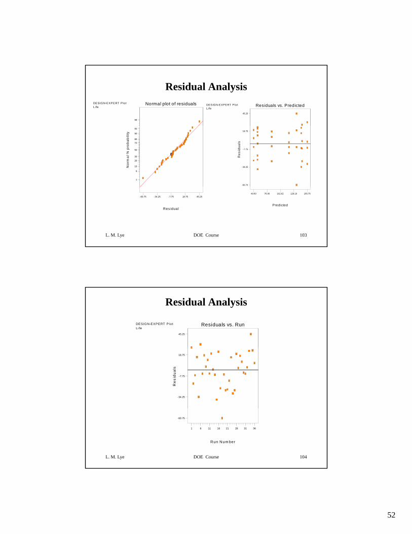
Residual Analysis DESIGN-EXPERT Plo tLi fe
Normal plot of residuals
99
DESIGN-EXPERT PlotL i fe
Residuals vs. Predicted
45.25
Nor
mal
% p
roba
bilit
y
1
5
10
20
30
50
70
80
90
95
Res
idua
ls
-60.75
-34.25
-7.75
18.75
L. M. Lye DOE Course 103
Res idual
-60.75 -34.25 -7.75 18.75 45.25
Predicted
49.50 76.06 102.62 129.19 155.75
Residual Analysis
DESIGN-EXPERT Plo tL i fe
Residuals vs. Run
45.25
Res
idua
ls
-34.25
-7.75
18.75
L. M. Lye DOE Course 104
Run Num ber
-60.75
1 6 11 16 21 26 31 36
53
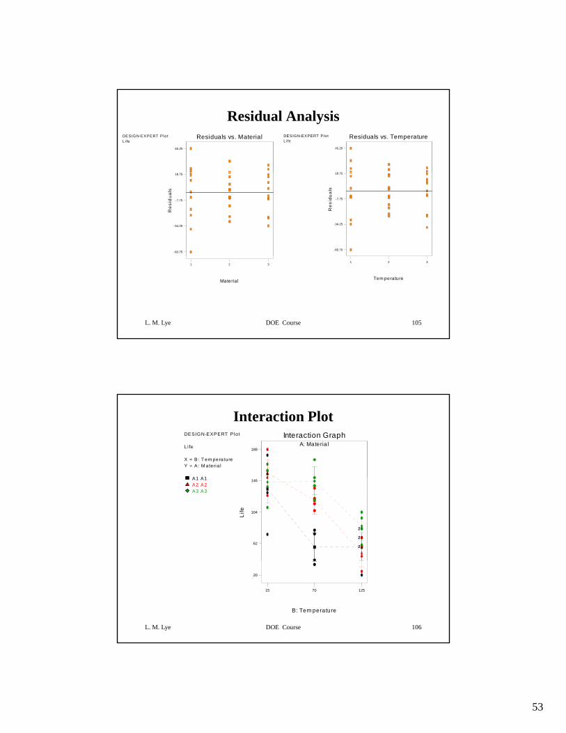
Residual Analysis DESIGN-EXPERT Plo tLi fe
Residuals vs. Material
45.25
DESIGN-EXPERT P lotL i fe
Residuals vs. Temperature
18 75
45.25
Res
idua
ls
-60.75
-34.25
-7.75
18.75
Res
idua
ls
-60.75
-34.25
-7.75
18.75
L. M. Lye DOE Course 105
Material
1 2 3
Tem perature
1 2 3
Interaction Plot DESIGN-EXPERT P lot
L i fe
X = B: T em peratureY = A: M ateria l
A1 A1
A: Materia lInteraction Graph
188
A1 A1A2 A2A3 A3
Life
62
104
146
2
2
22
2
2
L. M. Lye DOE Course 106
B: Tem perature
15 70 125
20
54
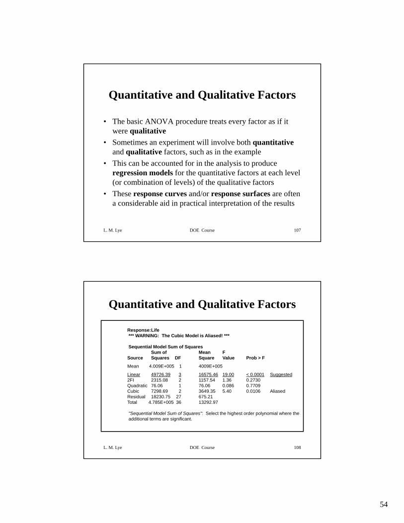
Quantitative and Qualitative Factors
• The basic ANOVA procedure treats every factor as if itThe basic ANOVA procedure treats every factor as if it were qualitative
• Sometimes an experiment will involve both quantitativeand qualitative factors, such as in the example
• This can be accounted for in the analysis to produce regression models for the quantitative factors at each level (or combination of levels) of the qualitative factors
L. M. Lye DOE Course 107
(or combination of levels) of the qualitative factors• These response curves and/or response surfaces are often
a considerable aid in practical interpretation of the results
Quantitative and Qualitative Factors
Response:Life*** WARNING: The Cubic Model is Aliased! ***
Sequential Model Sum of SquaresSum of Mean F
Source Squares DF Square Value Prob > F
Mean 4.009E+005 1 4009E+005
Linear 49726.39 3 16575.46 19.00 < 0.0001 Suggested2FI 2315.08 2 1157.54 1.36 0.2730Quadratic 76.06 1 76.06 0.086 0.7709Cubic 7298.69 2 3649.35 5.40 0.0106 AliasedResidual 18230.75 27 675.21
L. M. Lye DOE Course 108
Total 4.785E+005 36 13292.97
"Sequential Model Sum of Squares": Select the highest order polynomial where theadditional terms are significant.
55
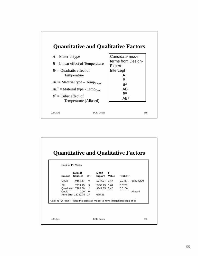
Quantitative and Qualitative FactorsCandidate model t f D i
A = Material typeterms from Design-Expert:Intercept
ABB2
AB
B = Linear effect of Temperature
B2 = Quadratic effect of Temperature
AB = Material type – TempLinear
AB2 = Material type Temp
L. M. Lye DOE Course 109
ABB3
AB2
AB = Material type - TempQuad
B3 = Cubic effect of Temperature (Aliased)
Quantitative and Qualitative Factors
Lack of Fit Tests
Sum of Mean FSource Squares DF Square Value Prob > F
Linear 9689.83 5 1937.97 2.87 0.0333 Suggested
2FI 7374.75 3 2458.25 3.64 0.0252Quadratic 7298.69 2 3649.35 5.40 0.0106Cubic 0.00 0 AliasedPure Error 18230.75 27 675.21
L. M. Lye DOE Course 110
"Lack of Fit Tests": Want the selected model to have insignificant lack-of-fit.
56
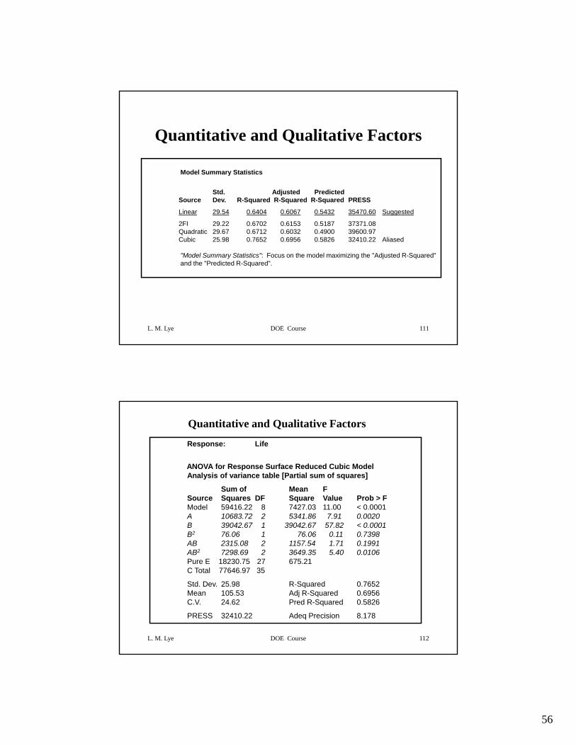
Quantitative and Qualitative Factors
Model Summary Statisticsy
Std. Adjusted PredictedSource Dev. R-Squared R-Squared R-Squared PRESS
Linear 29.54 0.6404 0.6067 0.5432 35470.60 Suggested
2FI 29.22 0.6702 0.6153 0.5187 37371.08Quadratic 29.67 0.6712 0.6032 0.4900 39600.97Cubic 25.98 0.7652 0.6956 0.5826 32410.22 Aliased
"Model Summary Statistics": Focus on the model maximizing the "Adjusted R-Squared"
L. M. Lye DOE Course 111
and the "Predicted R-Squared".
Quantitative and Qualitative Factors
Response: Life
ANOVA for Response Surface Reduced Cubic ModelAnalysis of variance table [Partial sum of squares]
Sum of Mean FSource Squares DF Square Value Prob > FModel 59416.22 8 7427.03 11.00 < 0.0001A 10683.72 2 5341.86 7.91 0.0020B 39042.67 1 39042.67 57.82 < 0.0001B2 76.06 1 76.06 0.11 0.7398AB 2315.08 2 1157.54 1.71 0.1991AB2 7298.69 2 3649.35 5.40 0.0106Pure E 18230.75 27 675.21C Total 77646 97 35
L. M. Lye DOE Course 112
C Total 77646.97 35
Std. Dev. 25.98 R-Squared 0.7652Mean 105.53 Adj R-Squared 0.6956C.V. 24.62 Pred R-Squared 0.5826
PRESS 32410.22 Adeq Precision 8.178
57
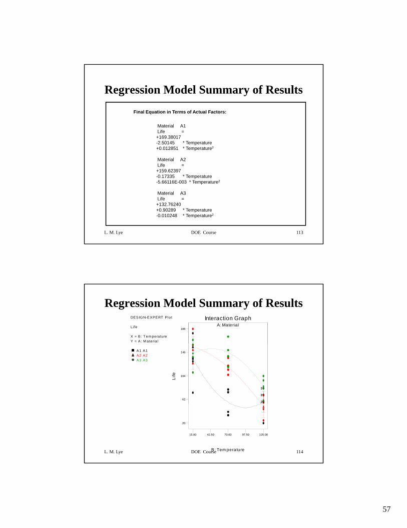
Regression Model Summary of Results
Final Equation in Terms of Actual Factors:
M i l A1Material A1Life =+169.38017-2.50145 * Temperature+0.012851 * Temperature2
Material A2Life =+159.62397-0.17335 * Temperature-5.66116E-003 * Temperature2
L. M. Lye DOE Course 113
p
Material A3Life =+132.76240+0.90289 * Temperature-0.010248 * Temperature2
Regression Model Summary of ResultsDESIGN-EXPERT Plo t
L i fe
X = B: T em peratureY = A: M ateria l
A: MaterialInteraction Graph
188
A1 A1A2 A2A3 A3
Life
62
104
146
2
2
22
2
2
L. M. Lye DOE Course 114B: Tem perature
15.00 42.50 70.00 97.50 125.00
20
58
Factorials with More Than Two Factors
• Basic procedure is similar to the two-factor case;• Basic procedure is similar to the two-factor case; all abc…kn treatment combinations are run in random order
• ANOVA identity is also similar:
T A B AB ACSS SS SS SS SS= + + + + +L L
L. M. Lye DOE Course 115
ABC AB K ESS SS SS+ + + +LL
More than 2 factors• With more than 2 factors, the most useful ,
type of experiment is the 2-level factorial experiment.
• Most efficient design (least runs)• Can add additional levels only if required
L. M. Lye DOE Course 116
• Can be done sequentially• That will be the next topic of discussion