Design and analysis of low frequency strut‐straddling feed arraysfor EVLA reflector antennas

M. Harun1 and S. W. Ellingson1

Received 15 March 2011; revised 18 July 2011; accepted 24 July 2011; published 18 October 2011.

[1] A new feed system is designed for operation below 100 MHz. The only existingsystem on the EVLA operating below 100 MHz is the “4 m” (74 MHz) system whichuses crossed half‐wave dipoles located in front of the Cassegrain subreflector as thefeed. However, the dipole feeds of this system introduce blockage, and a reduction insystem sensitivity (estimated to be ∼6% at 1.4 GHz) is observed at higher frequency bands;hence the dipoles are removed most of the time. An alternative feed concept is thereforeproposed in this paper. The proposed system appears to reduce sensitivity degradation at1.4 GHz by 3% and thus might be permanently mounted. Moreover, the new system hassensitivity comparable to the existing system at frequencies below 100 MHz. The feed forthis system consists of dipoles mounted between the adjacent struts of the reflector and isthus referred to as a strut‐straddling feed array. This design and the analysis methodologyused in this paper should be applicable in meeting the contiguous frequency coveragerequirement (50–470MHz) of the new low frequency system proposed for the EVLA. Also,it may be applied in the modification of other existing large reflector antennas for lowfrequency operation.

Citation: Harun, M., and S. W. Ellingson (2011), Design and analysis of low frequency strut‐straddling feed arrays for EVLAreflector antennas, Radio Sci., 46, RS0M04, doi:10.1029/2011RS004710.

1. Introduction

[2] The Expanded Very Large Array (EVLA) consists of27 Cassegrain reflector antennas on the Plains of SanAgustin, New Mexico. Each reflector antenna is 25 metersin diameter, and has a focal length (f) to diameter (D) ratioof 0.36. An EVLA reflector antenna is shown in Figure 1.The original design included capabilities at four bandscorresponding to wavelengths of 21 cm (≈1.4 GHz), 6 cm(5 GHz), 2 cm (15 GHz), and 1.3 cm (23 GHz) [Napieret al., 1983]. The first low frequency system, operating at90 cm, was installed in 1989. This system employed crosseddipoles mounted in front of the Cassegrain subreflector asthe feed. The success of the 90 cm system led to the con-sideration of a lower‐frequency capability. The “4 m” systemoperating at 74 MHz was thus installed, and is described byKassim et al. [1993, 2007]. The feed for this system alsoconsists of crossed half‐wave dipoles in front of the subre-flector, and yields an aperture efficiency of somewhere in therange 15% [Kassim et al., 1993] to 25% [Kassim et al., 2007].Blockage and scattering from the 4 m system reduces thesensitivity of the 21 cm system by about 6% [Kassim et al.,1993]; thus, the dipoles are not permanently installed andare only intermittently used.

[3] A new “low frequency system” (LFS) with the goal ofcovering 50–470 MHz has been proposed for the EVLA[Ott et al., 2009]. Additional feeds will probably be requiredto accommodate this frequency range. In this paper, wefocus our interest in covering the frequency range below100 MHz. Traditional approaches to feed design for cov-ering large tuning ranges focus on achieving large imped-ance bandwidth which results in large, complex feeds, e.g.,the Eleven feed [Olsson et al., 2006]. However, in the fre-quency regime of our interest, simple dipole‐like antennascan offer large usable bandwidth from a sensitivity perspec-tive. This is because at these frequencies, Galactic noise caneasily dominate over the self‐noise of the electronicsconnected to the antenna. Once the system is Galactic noise‐limited, improving the impedance matching between theantenna and the connected electronics does not significantlyimprove sensitivity [Ellingson, 2005]. As a result, the usablebandwidth for a dipole‐like antenna under these conditionstends to be much larger than its narrow impedancebandwidth. For example, Ellingson et al. [2007] show that a38 MHz resonant dipole with a 300 K front end achievesGalactic noise‐limited sensitivity over the range of 29–47 MHz at least.[4] The notion of low frequency feeds for large reflector

antennas is not new; however prior work did not allowsimultaneous operation with L‐band and higher‐frequencysystems. For example, the 50 MHz system employed on theGMRT employs dipoles as a low frequency feed; this feed isco‐located with the existing 327 MHz feed. However, the50‐ and 327‐MHz dipoles are located above a 3 m × 3 m

1Bradley Department of Electrical and Computer Engineering, VirginiaTech, Blacksburg, Virginia, USA.

Copyright 2011 by the American Geophysical Union.0048‐6604/11/2011RS004710

RADIO SCIENCE, VOL. 46, RS0M04, doi:10.1029/2011RS004710, 2011

RS0M04 1 of 12

square reflector which must be rotated out of position inorder for higher frequencies to be used [Shankar et al.,2009]. A low frequency system employing retractable fol-ded dipole feeds was briefly installed on the WSRT foroperation from 110 to 190 MHz [van der Marel et al.,2005].[5] In this paper, we first characterize the performance of

the existing EVLA 4 m system in the range 50–88 MHz.

Then, in order to resolve the blockage issue associated withthe existing system, we propose a new feed consisting of aring of dipoles mounted between adjacent struts. Thisarrangement is referred to as a strut‐straddling feed array.The motivation behind this design is the fact that, at lowfrequencies, the available power in the volume in front of areflector spreads out from the focal region. As an example,the distribution of power density (co‐pol) in the focal planeof a simple 25 m diameter paraboloidal reflector upon aplane wave incidence at 500 MHz and 50 MHz are shown inFigures 2 and 3, respectively. It can be seen that the avail-able power spreads out significantly as the frequency islowered from 500 MHz to 50 MHz. As a result, even if wemove about 2 m away from the focus, the amount ofavailable power drops only by about half at 50 MHz. Thissuggests the possibility of absorbing an appreciable amountof power by employing an array of feeds away from thefocal region, and appropriately combining the signals fromthese feeds. Based on this philosophy, we show in this paperthat the new system offers sensitivity comparable to theEVLA 4 m system in the frequency regime below 100 MHz,but with reduced blockage (∼3% improvement) at higherfrequency bands.[6] The rest of this paper is organized as follows. Section 2

describes the methodology used to analyze the sensitivity ofa reflector antenna. Sensitivity is expressed in terms of thesystem equivalent flux density (SEFD), which is defined asthe flux spectral density (W m−2 Hz−1) which yields signal‐to‐noise ratio (SNR) of unity at the output of the system.Section 3 describes the electromagnetic modeling of anEVLA reflector antenna required for analysis using the

Figure 1. An EVLA reflector antenna. Image source isNRAO/AUI, P. A. Lofy, Photographer. Available at http://images.nrao.edu/Telescopes/VLA/480.

Figure 2. Distribution of power density in the focal plane of a reflecting paraboloid (D = 25 m,f/D = 0.36) relative to the power density at the focus at 500 MHz.

HARUN AND ELLINGSON: STRUT‐STRADDLING FEED RS0M04RS0M04

2 of 12

method of moments (MoM). The findings of sections 2 and 3are then applied in section 4 to estimate the sensitivity of theexisting EVLA 4 m system. An analysis of sensitivity of theEVLA 4 m system as presented in this section has not beenpreviously reported to the best of our knowledge. Section 5describes the strut‐straddling feed array design, and com-pares the sensitivity and associated blockage of the newsystem with the existing system. Conclusions are summa-rized in section 6.

2. Methodology for Analysis of the Sensitivityof Dipole Arrays Used as a Reflector Feed

[7] The metric used in this paper for evaluating the per-formance of low frequency systems is sensitivity. Sensitivityis expressed in terms of SEFD. SEFD is a useful metric as itincludes the combined effect of the feed antennas and allsources of noise into a single number that is directly relatedto the sensitivity of astronomical observations. A detailedformulation of SEFD for analyzing low frequency systemsis presented in this section. An important aspect of thisformulation is that the correlation of external noise betweenthe array elements is not ignored. The correlation of externalnoise can significantly desensitize the system [Ellingson,2011]. This is more of a concern at low frequencies wherethe external noise can easily dominate the internal noise ofthe system. Therefore, the particular formulation of SEFDpresented in this paper is different from most other for-mulations, and feeds our purpose of evaluating low fre-quency systems. Part of the formulation provided in thissection is given by Ellingson [2011]; however, it is stillpresented here briefly, since some of the intermediate resultsare used for the analysis.

[8] Let E�(t) and E�(t) be the �‐ and �‐polarized com-ponents of the electric field associated with the signal of ourinterest, incident from a direction of {�0, �0}, having unitsof V m−1 Hz−1/2. The direction {�0, �0} will be representedas y0 henceforth. The resulting voltage at the terminals ofthe nth feed antenna, having units of V Hz−1/2, is

xn tð Þ ¼ a�n 0ð ÞE� tð Þ þ a�n 0ð ÞE� tð Þ þ zn tð Þ þ un tð Þ ð1Þ

where an�(y0) and an

�(y0) are the effective lengths, havingunits of meters, associated with the � and � polarizationsrespectively, for the nth feed antenna for a plane waveincident from y0; zn(t) is the contribution from noiseexternal to the system; and un(t) is the contribution fromnoise internal to the system. When the signals from all thefeed antennas are combined, the output can be expressed as

y tð Þ ¼XNn¼1

bnxn tð Þ ð2Þ

where N is the number of feed antennas, and the unitlessbn’s are the combining coefficients. In this paper, we assumeeach dipole is connected to a receive path that is fullycharacterized in terms of its input impedance, RL, and itsinput‐referred noise temperature, Tp. One way this could berealized is to use an “active balun” which presents a dif-ferential input impedance of RL to the dipole, a single‐endedoutput to a coaxial cable, and provides gain sufficient todominate the input‐referred noise temperature. This schemeis described by Ellingson et al. [2007, 2009] and Ellingson[2011]. The beam‐forming coefficients can be implemented

Figure 3. Distribution of power density in the focal plane of a reflecting paraboloid (D = 25 m,f/D = 0.36) relative to the power density at the focus at 50 MHz.

HARUN AND ELLINGSON: STRUT‐STRADDLING FEED RS0M04RS0M04

3 of 12

by varying the length or phase of the cables before an analogcombiner, or the signals from the cables can be digitizedindividually and combined digitally.[9] Assuming root‐mean square voltages, the available

power at the output of the combiner is

Py ¼ y tð Þy* tð Þh iR�10 ð3Þ

where angle brackets denote time domain averaging, aster-isk denotes conjugation and R0 is the impedance lookinginto the system as seen from the terminals across which y(t)is measured. We will now expand equation (3) with theassumptions that the signal of interest, zn(t) and un(t) aremutually uncorrelated for any given n; i.e., for any n and m,

E� tð Þz*n tð ÞD E

¼ E� tð Þz*n tð ÞD E

¼ 0 ð4Þ

E� tð Þu*n tð ÞD E

¼ E� tð Þu*n tð ÞD E

¼ 0 and ð5Þ

zn tð Þu*m tð ÞD E

¼ 0 ð6Þ

The correlation of external noise between antennas is notprecluded by the above assumption since hzn(t)zm* (t)i can be≠0 for n ≠ m. Furthermore no assumption has been madeabout the correlation between E�(t) and E�(t). Upon expandingequation (3) we obtain

PyRo ¼ bHA��bP�� þ bHA��bP�� þ bHA��bP�� þ bHA��bP��

þ bHPzbþ bHPub ð7Þ

where “ H ” denotes the conjugate transpose operator;

b ¼ b1 b2 :: bN½ �T ð8Þ

where superscript T denotes the transpose operator; and

A�� ¼ a*� oð ÞaT� oð Þ P�� ¼ jE� tð Þj2D E

ð9Þ

A�� ¼ a*� oð ÞaT� oð Þ P�� ¼ jE� tð Þj2D E

ð10Þ

A�� ¼ a*� oð ÞaT� oð Þ P�� ¼ E� tð ÞE*� tð ÞD E

ð11Þ

A�� ¼ a*� oð ÞaT� oð Þ P�� ¼ E� tð ÞE*� tð ÞD E

ð12Þ

a� oð Þ ¼ a�1 oð Þ a�2 oð Þ . . . a�N oð Þ� �Tand ð13Þ

a� oð Þ ¼ a�1 oð Þ a�2 oð Þ . . . a�N oð Þh iT

ð14Þ

However, for an unpolarized signal of interest P�� = P�� = 0and P�� = P�� = hS(y)/2, where S(y) is the flux densityassociated with the signal.[10] Pz in equation (7) is a matrix whose (n, m)th element

is hzn*(t)zm(t)i, and Pu is a matrix whose (n, m)th element

is hun*(t)um(t)i. We now find a simple expression for the(n, m)th element of Pz. The power in two polarizations ofthe electric field associated with the unpolarized externalnoise incident from a region of solid angleDW around y canbe expressed as

jDE� ; tð Þj2D E

¼ jDE� ; tð Þj2D E

¼ �

2DS ð Þ ð15Þ

where h is impedance of free space and DS(y) is theassociated flux density having units of W m−2 Hz−1. DS(y)can be obtained from Rayleigh‐Jeans Law:

DS ð Þ ¼ 2k

�2Tb ð ÞDW ð16Þ

where Tb(y) is the brightness temperature in the direction y,and l is wavelength. We can thus model DE�(y, t) andDE�(y, t) as follows:

DE� ; tð Þ ¼ g� ; tð Þffiffiffiffiffiffiffiffiffiffiffiffiffiffiffiffiffiffiffiffiffiffiffiffiffik�

�2Tb ð ÞDW

rð17Þ

DE� ; tð Þ ¼ g� ; tð Þffiffiffiffiffiffiffiffiffiffiffiffiffiffiffiffiffiffiffiffiffiffiffiffiffik�

�2Tb ð ÞDW

rð18Þ

where g�(y, t) and g�(y, t) are Gaussian‐distributed inde-pendent random variables with zero mean and unit variance.Now, in order to obtain zn(t) we sum the contributionsreceived over a sphere:

zn tð Þ ¼X

a�n ð ÞDE� ; tð Þ þ a�n ð ÞDE� ; tð Þ� � ð19Þ

Applying the definition of Pz and exploiting the statisticalproperties of g�(y, t) and g�(y, t) we find

P n;m½ �z ¼ k�

�2

X

a�*n ð Þa�m ð Þ þ a�*n ð Þa�m ð Þh i

Tb ð ÞDW ð20Þ

Returning to equation (7), we obtain the following expres-sion for the signal‐to‐noise ratio (SNR) for an unpolarizedsignal of interest:

SNR ¼ �

2S ð Þ b

H A�� þ A��

� �b

bH Pz þ Puð Þb ð21Þ

The maximum possible SNR is equal to the maximumeigenvalue of Rn

−1Rs [Monzingo and Miller, 1980], where

Rn ¼ Pz þ Pu and ð22Þ

Rs ¼ A��P�� þ A��P�� ð23Þ

The maximum SNR is achieved by selecting b to be theeigenvector corresponding to the maximum eigenvalue ofRn−1Rs. To summarize, the procedure to compute the optimal

beam‐forming cofficients (bn’s) is as follows: (1) computeRs using equations (9), (10) and (23); (2) compute Rn usingequation (22), and (3) compute b = Rn

−1Rs. Note that P�� andP�� may be taken to be unity for simplicity, since thesevalues merely scale b, which has no impact on SNR. Pz in

HARUN AND ELLINGSON: STRUT‐STRADDLING FEED RS0M04RS0M04

4 of 12

equation (22) may be obtained either by direct measurement(using the definition of Pz), or by simulation as implied byequation (20). Similarly, Pu in equation (22) can be obtainedeither by measurement or from advance knowledge of thereceiver temperatures.[11] Regardless of the choice of b, the sensitivity of the

antenna system can now be expressed in terms of SEFD,which is the value of S(y) that gives an SNR of 1; i.e.,

SEFD ¼ 2

�

bH Pz þ Puð ÞbbH A�� þ A��

� �b

ð24Þ

Note that this expression gives SEFD directly in terms offeed element effective lengths (i.e., gains), external andinternal noise powers, and the combining coefficients.

3. Electromagnetic Modeling of an EVLAReflector Antenna

[12] In this section, we describe an electromagnetic modelof an EVLA reflector antenna. In our frequency range ofinterest, the reflector is not very large compared to awavelength, and therefore requires “full‐wave” analysis(e.g., MoM) for accurate results. In this paper, we employ theNEC2 implementation ofMoM [Burke and Poggio, 1981] forthis purpose.[13] The major parts of an EVLA reflector antenna are:

main reflector, subreflector, struts, support wires, subre-flector mount, and high‐frequency feed assembly. Figure 4shows a drawing of these components (minus the mainreflector) along with their dimensions. Study shows that allthese components have impact on the gain and pattern of thereflector antenna [Harun and Ellingson, 2008]. Therefore,an accurate model of an EVLA antenna should include all ofthese components.[14] The main reflector is modeled as a wire grid. The grid

spacing (smallest distance between two parallel wires in thegrid) and the wire radius are selected based on a simpleexperiment. A wire grid model of a flat disk of diameter 25 mis used as a ground plane, and a half‐wave dipole is locatedquarter wavelength (at 74 MHz) above this grid. The gridspacing and wire radius are then varied to achieve a per-formance (gain and pattern) which is comparable to theperformance observed when the grid is replaced by a perfectsolid ground plane. Experiments showed that a wire gridwith grid spacing of 36.5 cm and wire radius of 45 mmachieves this criterion while using a manageable number ofsegments.[15] In the model used in this paper, the main reflector is

centered around the z‐axis of the coordinate system with itscircumference parallel to the xy‐plane, and the prime focuscoincides with the origin of the coordinate system. We willrefer to this coordinate system in the rest of this paper foridentifying different locations in the antenna model. Themain reflector model consists of the wire grid (as determinedin the previous paragraph) paraboloid with f/D = 0.36, andD = 25 m.[16] The subreflector has a diameter of 2.35 m. Its shape is

not known to us in detail; however a drawing of the sub-reflector was made available to us. Using the drawing we

extracted data points along the cross section of the subre-flector and used a polynomial equation to fit the data withina residual (difference between the data point and the pre-dicted value from the polynomial equation) of 0.01l at74 MHz. From this we created a wire grid model for thesubreflector in the same manner as the main reflector. Wedid not use the same grid spacing as the main reflector, asthis spacing is very large with respect to the diameter of thesubreflector, and results in excessively large “quantizationerror” in the rim of the subreflector. Therefore, we used asmaller grid spacing of 12 cm to reduce the error. Also, inthe complete antenna model the subreflector is not sym-metrical about the axis of the reflector; it is slightly tilted.This is because in the actual EVLA antenna the subreflectoris tilted in order to point toward feeds arranged in a ring nearthe vertex of the main reflector.[17] The largest dimension of the cross section of a strut is

40 cm, which at 74 MHz is 0.1l. We could model the strutas a single wire according to the Equal Area Rule[Rubinstein et al., 2005], but in our case the radius of the wirewould be 10 cm, which is larger than l/(20p) at 74 MHz andtherefore not appropriate according to the modeling guide-lines of NEC2. Instead, we model the strut as two wires ofradius 3 cm placed 40 cm apart, with connecting segmentsevery 50 cm.[18] The four support wires are modeled using single wires

of radius 1 cm, having segment lengths ≈ l/10 at 74 MHz.[19] The subreflector mount is modeled as a wire grid

cylinder (visible in Figure 5). The top and bottom surfacesof the cylinder are modeled using concentric rings separatedby a distance of l/10 at 74 MHz. Radial wires with segmentlengths of l/10 are then created to connect the concentricrings. As for the cylindrical surface, two more circular ringsare created in between the top and the bottom surfaces.These rings are then connected to the top and the bottomsurfaces, and to each other using vertical wires of segmentlength l/10.[20] The high‐frequency feed assembly at the center of the

main reflector is modeled as a wire grid rectangular box.The grid spacing and wire radius of this rectangular box isthe same as that used for modeling the main reflector.[21] We modeled the dipoles of the existing 4 m system

using single wires having 11 segments. The radius of eachof the dipoles is 2.38 mm, and the length is selected to be1.94 m to make it resonate at 74 MHz.[22] The wire grid model explained above was developed

so that the total number of segments at 74 MHz is less than11,000 and can fit in 2 GB of RAM. However, the modelmeets the NEC2 modeling guidelines up to 100 MHz.[23] In order to check the validity of the model we analyze

the gain and pattern of the EVLA 4 m system at 74 MHz. Inthis analysis, only one dipole feed is considered at a time.The dipole is located at the image (as reflected by thesubreflector) of the prime focus. The support wires may beoriented in two different ways with respect to a dipole feed,as shown in Figures 5 and 6, and have different impacts onthe gain and the pattern. One of these orientations is whenthe wires are roughly aligned with the dipole; this will bereferred to as the co‐aligned orientation (Figure 5). Theother orientation is when the wires are roughly cross‐alignedwith the dipole; this will be referred to as the cross‐alignedorientation (Figure 6).

HARUN AND ELLINGSON: STRUT‐STRADDLING FEED RS0M04RS0M04

5 of 12

[24] The results of our analysis are shown in Figures 7and 8 for the two possible orientations of the support wires.First, we consider the performance of the dipole which isco‐aligned with the support wires (shown in Figure 7). Notethe gain (G) at 74 MHz is predicted to be 20.4 dB whichcorresponds to an aperture efficiency of 29%. The apertureefficiency, �a is calculated as the ratio of the effectiveaperture, Ae (Ae = Gl2/4p) and the physical aperture (pD2/4)of the antenna. The gain of the cross‐aligned dipole (Figure 8)at 74 MHz is found to be 16.2 dB, i.e., 4 dB worse, corre-sponding to �a = 11%. This is apparently due to an unfavor-able interaction with the support wires in this configuration.This difference between the co‐ and cross‐aligned dipoles has

been observed in practice, but is difficult to quantify (F. N.Owen, National Radio Astronomy Observatory, privatecommunication, September 2010). It is interesting to note thatour estimates of 29% and 11% are consistent with the esti-mates of 25% and 15% reported by Kassim et al. [1993] andKassim et al. [2007], respectively, although it is not clear ifthe latter pertains to different feed dipole orientations, asconsidered here.[25] Also visible in Figures 7 and 8 is the fact that the

pattern of the antenna system has slight asymmetry. This isbecause the subreflector is tilted as described in section 2.[26] The consistency of the simulated results with what is

observed in practice gives us confidence in the model. Using

Figure 4. Detail of an EVLA reflector antenna geometry, showing the subreflector, the subreflectormount, the struts, the support wires and the feed assembly. The drawing is provided by J. Ruff of NRAO.

Figure 5. Orientation of the support wires in the EVLAantenna model with respect to a single co‐aligned dipolefeed.

Figure 6. Orientation of the support wires in the EVLAantenna model with respect to a single cross‐aligned dipolefeed.

HARUN AND ELLINGSON: STRUT‐STRADDLING FEED RS0M04RS0M04

6 of 12

this model the sensitivities of an EVLA antenna for theexisting 4 m system, and for the proposed new system, areanalyzed in sections 4 and 5, respectively.

4. Analysis of Sensitivity of the ExistingEVLA 4 m System

[27] In this section, we estimate the sensitivity of theEVLA 4 m system in terms of SEFD. In order to compute

the effective lengths of the feed dipoles, the completereflector antenna model is illuminated with a �‐polarized1 V/m plane wave incident from some direction y, and theresulting current IL across a series resistance RL at the feedterminals is determined using MoM. a�(y) for the feedantenna is then simply ILRL. The process is repeated for a�‐polarized plane wave and iterated over y.[28] The internal noise covariance matrix Pu is computed

assuming that the internal noise between feed antennas is

Figure 7. Calculated E‐plane co‐pol gain of the EVLA 4 m system for co‐aligned support wires.

Figure 8. Calculated E‐plane co‐pol gain of the EVLA 4 m system for cross‐aligned support wires.

HARUN AND ELLINGSON: STRUT‐STRADDLING FEED RS0M04RS0M04

7 of 12

not correlated, so that Pu becomes a diagonal matrix whosenon‐zero elements are

P n½ �u ¼ kTp;nRL ð25Þ

where k is Boltzmann’s constant (1.38 × 10−23 J/K), and Tp,nis the input‐referred internal noise temperature associatedwith the nth antenna. In this paper, it is assumed that RL =100 W, and Tp,n = Tp = 250 K. These values are selected tobe comparable to existing low frequency telescope systemsthat employ dipole‐like antennas, e.g., the LWA [Ellingsonet al., 2009], as opposed to the actual 4 m system receivertemperature, which is significantly higher.[29] The external noise covariance matrix, Pz is computed

using equation (20), where Tb(y) is obtained using a modelproposed by Ellingson [2005]. In this model Tb(y) is

assumed to be uniform over the sky (� < p/2) and zero for� > p/2. Using this model Tb(y) toward the sky is foundto be 4835 K, 3035 K, 1777 K, and 1142 K at 50 MHz,60 MHz, 74 MHz and 88 MHz respectively. The actualcontributions to system temperature are less due to theimpedance mismatch between the antenna self‐impedanceand RL. This mismatch is automatically taken into account inthe way we determine the effective lengths of the feedantenna. The signals from the two crossed dipoles arecombined to obtain circular polarization.[30] The results of our analysis are shown in Figure 9.

SEFD estimations for the system are calculated only in therange 50‐88 MHz. Due to the presence of interference fromthe FM broadcast band, the range 88–100 MHz is notconsidered in this paper. As can be seen from Figure 9,SEFD increases (i.e., becomes worse) below 70 MHz. Thereason for this is the fact that the impedance mismatch startsto become so bad that the system no longer remainsGalactic‐noise limited, and the internal noise starts to definethe sensitivity. The ratio of Tr{Pz}/Tr{Pu} (where “Tr”denotes the trace operation; i.e., the sum of the diagonalterms.) expresses the degree by which Galactic noise dom-inates the internal noise at the combined output, and isshown in the inset of Figure 9.

5. Strut‐Straddling Feed Array

[31] In this section, we consider the strut‐straddling feedarray. In this arrangement the dipoles are mounted in a ring‐like formation between adjacent struts as shown in Figure 10.The radii of these dipoles are selected to be 4.76mm, and theirlengths are determined to make them resonant at 74 MHz.The radius is increased from that of the existing dipoles(2.38 mm) in order to improve the impedance bandwidth; sothat we can achieve Galactic noise‐limited sensitivity over awider tuning range without making major changes to theshape and size of the feed. The signal path is modeled suchthat the signals from the dipoles and their associated elec-tronics are multiplied by combining coefficients that maxi-mize the SNR, and the products are summed into a single

Figure 9. Estimated SEFD for the existing EVLA 4 msystem. The inset table shows degree of Galactic noisedominance.

Figure 10. Single ring strut‐straddling feed array.

Figure 11. Location selection for mounting strut‐straddlingfeed array based on SEFD at 74 MHz. Dashed line is theSEFD of the existing EVLA 4 m system at 74 MHz.

HARUN AND ELLINGSON: STRUT‐STRADDLING FEED RS0M04RS0M04

8 of 12

output. To properly consider the broadband performance, thecombining coefficients are recomputed at each frequency ofinterest.[32] A key design parameter in this scheme is the location

of the plane in which the ring of dipoles will be located. Weconsidered planes from z = −0.25 m to z = −4.0 m in incre-ments of 0.25 m. The study is limited within these locationsdue to the huge computational burden involved with theanalysis (a single‐frequency simulation requires about 3 hoursin a 2.33 GHz quad‐core processor machine). In each ofthese planes we employed the ring of dipoles, and calculated

the SEFD at 74 MHz. The results are shown in Figure 11.The lowest SEFD at 74 MHz is observed for dipoles in theplane z = −1.0 m at which the SEFD is within 10% of thatfor the existing 4 m system. This location is thereforeselected as the preferred location for mounting a single ringof strut‐straddling dipoles. The second lowest SEFD isobserved at z = −2.25 m, and is comparably low. Thissuggests the possible utility of a second ring of dipoles.[33] The SEFD for the new system with a single ring of

dipoles at z = −1.0 m are estimated and compared with theEVLA 4 m system. The results are shown in Figure 12.

Figure 12. Estimated SEFD for a single ring of strut‐straddling dipoles at z = −1.0 m, and comparisonwith the existing EVLA 4 m system.

Figure 13. Propagation paths in a Cassegrain reflector antenna in transmit mode, corresponding toEVLA operation at wavelengths of 21 cm and below.

HARUN AND ELLINGSON: STRUT‐STRADDLING FEED RS0M04RS0M04

9 of 12

It can be observed that the new system has comparableperformance to the existing system; and in the range 55–65MHzthe new system performs better. At 74 MHz the new systemyields SEFD ≈ 53 kJy whereas the existing system yieldsSEFD ≈ 60 kJy.[34] In order to quantify the blocking by the dipole feeds,

we first identify three different paths of propagation in aCassegrain reflector antenna, corresponding to EVLAoperation at wavelengths of 21 cm or below. This is shownin Figure 13. The first path F ′S is from the secondary focus

to the subreflector. The second path SR is from the sub-reflector to the main reflector. The third path RA is from themain reflector toward the far field. In order to estimate theblockage in the first two paths, the field incident on the mainreflector due to a feed located at the secondary focus iscalculated using MoM. The analysis is performed separatelyfor the cases when blocking dipoles are present at the imageof the prime focus, and when the dipoles are mountedbetween adjacent struts. For both of these cases, the resultingphysical optics currents on the reflector surface are calcu-lated, and then radiated to find the directivity of the system.When the dipoles located at the image of the prime focus arereplaced with a single ring of strut‐straddling dipoles at z =−1.0 m, the effective aperture is seen to increase by 3.7% at1.4 GHz. Therefore, blockage at 1.4 GHz is significantlyreduced in the paths F ′S and SR when the new feed system isemployed.[35] In the above analysis blockage in the path RA is not

considered. In order to quantify blockage in this path at1.4 GHz, we need to compute the fields reflected from themain reflector, upon the excitation of a feed located at thesecondary focus, and the interaction of these fields withthe scattering objects (struts, subreflector, blocking dipoles)present in front of the main reflector. This requires a fullwave analysis at 1.4 GHz, which is not practical. Therefore,it is difficult to accurately quantify blockage in the path RA.However, an approximate study to compare the blockage inthis path due to the strut‐straddling dipoles and the imageprime focus dipoles is possible. In this study, we illuminatethe entire structure in front of the main reflector, but in theabsence of the main reflector, with an uniform plane waveincident from the negative z‐axis, both for the cases whenthe blocking dipoles are present at the image of the primefocus, and when the dipoles are mounted between adjacentstruts. The scattering cross section in the forward direction is

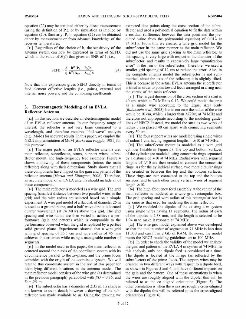
Figure 14. Double ring strut‐straddling feed array.

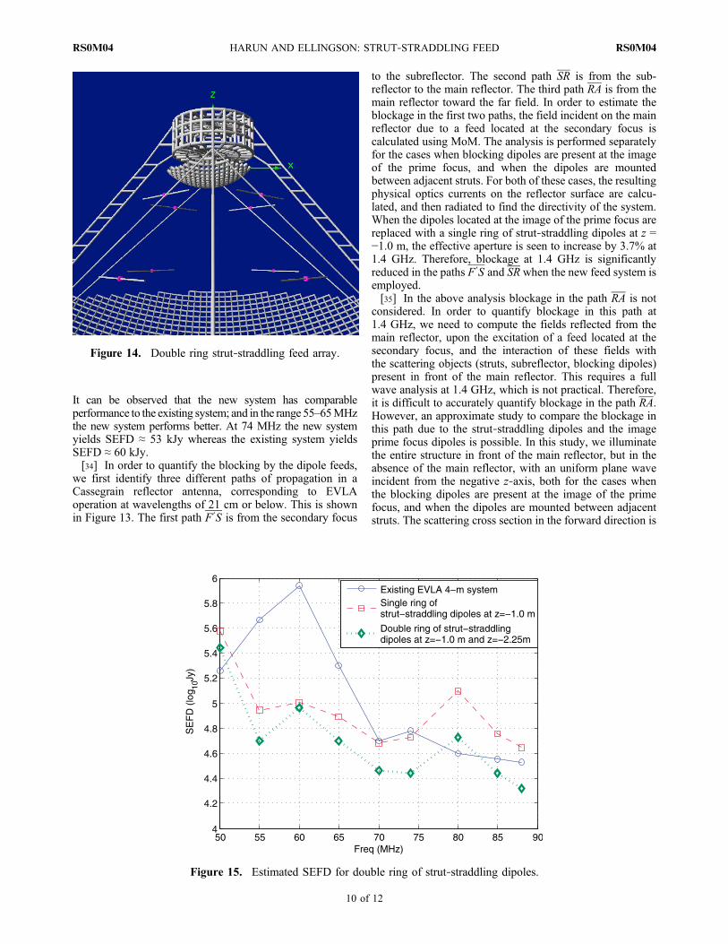
Figure 15. Estimated SEFD for double ring of strut‐straddling dipoles.

HARUN AND ELLINGSON: STRUT‐STRADDLING FEED RS0M04RS0M04

10 of 12

then calculated. It is observed that when the dipoles locatedat the image of the prime focus are replaced with the strut‐straddling dipoles at z = −1.0 m, the scattering cross sectionincreases by about 3%. However, in this case the scatteringcross section is computed assuming an uniform plane wave,whereas in practice a non‐uniform plane wave is producedupon reflection from the main reflector due to the sphericalspreading of the feed pattern incident on it. In fact, thepower density of the field reflected from the reflector sur-face is at least 3% higher along the z‐axis than at thelocation of the strut‐straddling dipoles. The increasedblockage due to increased scattering from the strut‐straddlingdipoles is approximately canceled by the reduced powerdensity of the incident field which they scatter. Thus, bothfeed systems introduce about the same blockage at 1.4 GHzalong the RA path.[36] Taking into account both the F ′SR and RA paths, we

estimate a reduction in blockage from about 6% (as esti-mated by Kassim et al. [1993]) for the existing 4 m systemto about 2.3% at 1.4 GHz using the strut‐straddling system.[37] A possible way to improve the sensitivity obtained

with a single ring of strut‐straddling dipoles without makingblockage worse is to use two rings, as shown in Figure 14.As pointed out earlier, z = −1.0 m and z = −2.25 m appear tobe the suitable choices for the locations of the two rings.Figure 15 shows the results for this arrangement. Again, thecombining coefficients are selected to maximize SNR. Notethat the SEFD for the double ring system is better than theexisting system at all the frequencies except for 50 and80 MHz. Again, in the same manner as described above, theblockage introduced by this system at 1.4 GHz is estimated.There is not any significant increase (less than 0.2%) in

blocking in the path F ′SR when the single ring of dipoles isreplaced by the double ring. Also, in the path RA theincrease in blockage is estimated to be negligible as thescattering cross section in the forward direction for thedouble ring is increased only by 4% from that of the singlering; whereas the incident power density in the location ofthe second ring (z = −2.25 m) is at least 4% less than that atthe location of the first ring (z = −1.0 m).[38] For design optimization purposes, it would be useful

to have a simple rule or guidelines for choosing the locationsfor rings of dipoles. Unfortunately, this does not appear tobe possible, due to the complex interactions between thedipoles and between the dipoles and the dish structure. Atpresent, this optimization appears to be possible only by trialand error.[39] The strut‐straddling feed arrays described above

demonstrated performance comparable to the existing sys-tem, but with reduced blockage. An issue of concern may bethe support structure for the dipoles and the blockageassociated with this support. The dipoles of strut‐straddlingarrays can be easily mounted and supported using non‐conducting rope between the struts. Also, the cables carry-ing the signals from the dipoles can run along these ropes tothe struts and then be brought along the struts to the back ofthe subreflector where they can be combined. In order toestimate the effect of the cables, we did a simple studywhere one end of each of the dipoles is extended to thenearest struts to model the cable, and the blocking in thepath F ′SRA is again computed. It is found that there is nosignificant increase (less than 0.2%) in blockage in the F ′SRpath for extending the dipoles. On the other hand, thescattering cross section in the forward direction is increased

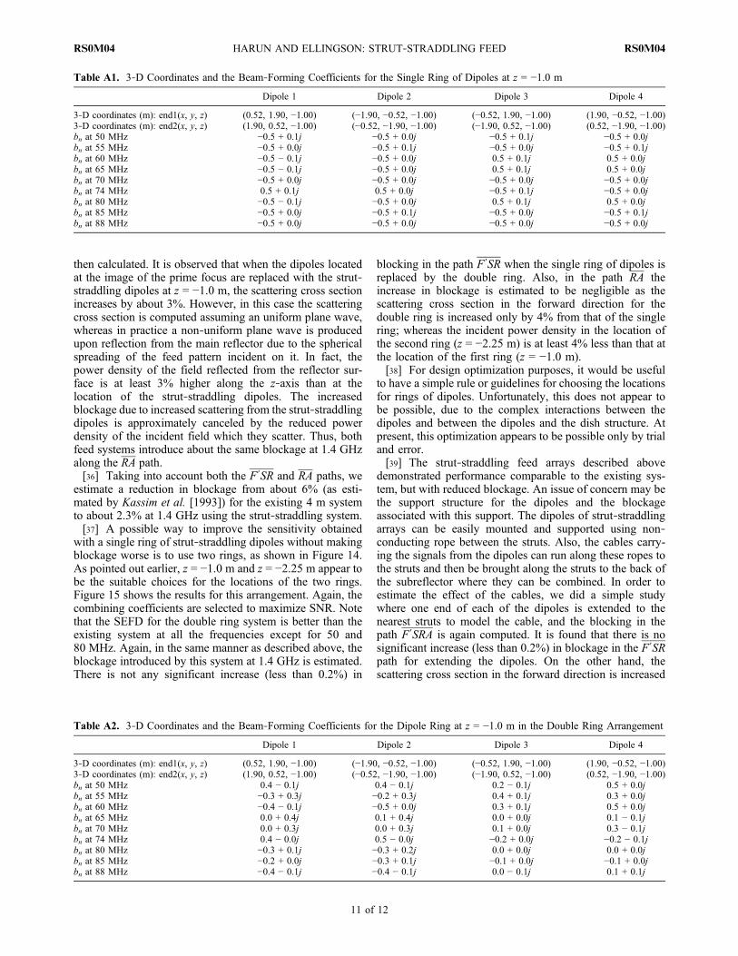
Table A1. 3‐D Coordinates and the Beam‐Forming Coefficients for the Single Ring of Dipoles at z = −1.0 m

Dipole 1 Dipole 2 Dipole 3 Dipole 4

3‐D coordinates (m): end1(x, y, z) (0.52, 1.90, −1.00) (−1.90, −0.52, −1.00) (−0.52, 1.90, −1.00) (1.90, −0.52, −1.00)3‐D coordinates (m): end2(x, y, z) (1.90, 0.52, −1.00) (−0.52, −1.90, −1.00) (−1.90, 0.52, −1.00) (0.52, −1.90, −1.00)bn at 50 MHz −0.5 + 0.1j −0.5 + 0.0j −0.5 + 0.1j −0.5 + 0.0jbn at 55 MHz −0.5 + 0.0j −0.5 + 0.1j −0.5 + 0.0j −0.5 + 0.1jbn at 60 MHz −0.5 − 0.1j −0.5 + 0.0j 0.5 + 0.1j 0.5 + 0.0jbn at 65 MHz −0.5 − 0.1j −0.5 + 0.0j 0.5 + 0.1j 0.5 + 0.0jbn at 70 MHz −0.5 + 0.0j −0.5 + 0.0j −0.5 + 0.0j −0.5 + 0.0jbn at 74 MHz 0.5 + 0.1j 0.5 + 0.0j −0.5 + 0.1j −0.5 + 0.0jbn at 80 MHz −0.5 − 0.1j −0.5 + 0.0j 0.5 + 0.1j 0.5 + 0.0jbn at 85 MHz −0.5 + 0.0j −0.5 + 0.1j −0.5 + 0.0j −0.5 + 0.1jbn at 88 MHz −0.5 + 0.0j −0.5 + 0.0j −0.5 + 0.0j −0.5 + 0.0j

Table A2. 3‐D Coordinates and the Beam‐Forming Coefficients for the Dipole Ring at z = −1.0 m in the Double Ring Arrangement

Dipole 1 Dipole 2 Dipole 3 Dipole 4

3‐D coordinates (m): end1(x, y, z) (0.52, 1.90, −1.00) (−1.90, −0.52, −1.00) (−0.52, 1.90, −1.00) (1.90, −0.52, −1.00)3‐D coordinates (m): end2(x, y, z) (1.90, 0.52, −1.00) (−0.52, −1.90, −1.00) (−1.90, 0.52, −1.00) (0.52, −1.90, −1.00)bn at 50 MHz 0.4 − 0.1j 0.4 − 0.1j 0.2 − 0.1j 0.5 + 0.0jbn at 55 MHz −0.3 + 0.3j −0.2 + 0.3j 0.4 + 0.1j 0.3 + 0.0jbn at 60 MHz −0.4 − 0.1j −0.5 + 0.0j 0.3 + 0.1j 0.5 + 0.0jbn at 65 MHz 0.0 + 0.4j 0.1 + 0.4j 0.0 + 0.0j 0.1 − 0.1jbn at 70 MHz 0.0 + 0.3j 0.0 + 0.3j 0.1 + 0.0j 0.3 − 0.1jbn at 74 MHz 0.4 − 0.0j 0.5 − 0.0j −0.2 + 0.0j −0.2 − 0.1jbn at 80 MHz −0.3 + 0.1j −0.3 + 0.2j 0.0 + 0.0j 0.0 + 0.0jbn at 85 MHz −0.2 + 0.0j −0.3 + 0.1j −0.1 + 0.0j −0.1 + 0.0jbn at 88 MHz −0.4 − 0.1j −0.4 − 0.1j 0.0 − 0.1j 0.1 + 0.1j

HARUN AND ELLINGSON: STRUT‐STRADDLING FEED RS0M04RS0M04

11 of 12

by about 1.5% when the dipoles are extended, and thusmight slightly increase the blockage. Nevertheless, the strut‐straddling dipoles with their supports are still estimated toreduce the blockage at 1.4 GHz relative to the image‐primefocus system.

6. Conclusion

[40] The performance of the existing EVLA 4 m system ischaracterized at frequencies below 100 MHz in terms ofSEFD. In order to overcome the blockage associated withthe existing feed system we proposed strut‐straddling feedarrays. Strut‐straddling feed arrays demonstrated perfor-mance comparable to or better than the existing image primefocus system in the frequency range about 50–90 MHz.Furthermore, our results indicate that this system achieves asignificant reduction in blockage at 1.4 GHz (wavelength of21 cm), possibly facilitating permanent installation.[41] Although the focus of this paper has been the EVLA,

the design technique and analysis methodology describedin this paper should be applicable to other large reflectorantennas as well.[42] The implementation described in this paper produces

a single polarization. Future work includes development ofcombining schemes to obtain dual orthogonal polarizations.

Appendix A: Beam‐Forming Coefficientsand Dipole Locations

[43] The beam‐forming coefficients and the 3‐D spatialcoordinates for the single ring of dipoles at z = −1.0 m aregiven in Table A1. Also, the beam‐forming coefficients andthe 3‐D spatial coordinates for the double ring of dipoles atz = −1.0 m, z = −2.25 m are given in Tables A2 and A3,respectively.

ReferencesBurke, G., and A. Poggio (1981), Numerical Electromagnetics Code (NEC)—Method of Moments, Part III: User’s Guide, Lawrence Livermore Lab,Livermore, Calif.

Ellingson, S. W. (2005), Antennas for the next generation of low‐frequencyradio telescopes, IEEE Trans. Antennas Propag., 53(8), 2480–2489,doi:10.1109/TAP.2005.852281.

Ellingson, S. W. (2011), Sensitivity of antenna arrays for long‐wavelengthradio astronomy, IEEE Trans. Antennas Propag., 59(6), 1855–1863,doi:10.1109/TAP.2011.2122230.

Ellingson, S. W., J. H. Simonetti, and C. D. Patterson (2007), Design andevaluation of an active antenna for a 29–47 MHz radio telescope array,IEEE Trans. Antennas Propag. , 55(3), 826–831, doi:10.1109/TAP.2007.891866.

Ellingson, S. W., et al. (2009), The long wavelength array, Proc. IEEE,97(8), 1421–1430, doi:10.1109/JPROC.2009.2015683.

Harun, M., and S. W. Ellingson (2008), Analysis of a dipole‐fed VLA dishbelow 100 MHz, technical report, Virginia Polytechnic Institute and StateUniversity.

Kassim, N. E., et al. (1993), Subarcminute resolution imaging ofradio sources at 74 MHz with the very large array, Astron. J., 106,2218–2228, doi:10.1086/116795.

Kassim, N. E., et al. (2007), The 74 MHz system on the very large array,Astrophys. J. Suppl. Ser., 172, 686–719, doi:10.1086/519022.

Monzingo, R. A., and T. W. Miller (1980), Introduction to Adaptive Arrays,John Wiley, New York.

Napier, P. J., et al. (1983), The very large array: Design and performance ofa modern synthesis radio telescope, Proc. IEEE, 71(11), 1295–1320,doi:10.1109/PROC.1983.12765.

Olsson, R., et al. (2006), The Eleven antenna: A compact decade bandwidthdual polarized feed for reflector antennas, IEEE Trans. Antennas Propag.,54(2), 368–375, doi:10.1109/TAP.2005.863392.

Ott, J., et al. (2009), Pushing the limits of the EVLA: An enhancement pro-gram for the next decade, Astro2010 activity white paper, Natl. Acad. ofSci., Washington, D. C. [Available at http://sites.nationalacademies.org/BPA/BPA_049855.]

Rubinstein, A., F. Rachidi, and M. Rubinstein (2005), On wire‐grid repre-sentation of solid metallic surfaces, IEEE Trans. Electromagn. Compat.,47(1), 192–195, doi:10.1109/TEMC.2004.838230.

Shankar, N. U., et al. (2009), A 50 MHz system for GMRT, in The Low‐Frequency Radio Universe, edited by D. J. Saikia, D. A. Green, andY. Gupta, Astron. Soc. Pac. Conf. Ser., 407, 393–397.

van der Marel, J., et al. (2005), Low frequency receivers for the WSRT:A window of opportunity, in Proceedings of URSI‐GA ’05, Int. Unionof Radio Sci., New Delhi, India. [Available at http://www.ursi.org/Proceedings/ProcGA05/pdf/J03-P.14(0817).pdf.]

S. W. Ellingson and M. Harun, Bradley Department of Electrical andComputer Engineering, Virginia Tech, 432 Durham, Blacksburg, VA 24060,USA. (ellingson@vt.edu; mharun@vt.edu)

Table A3. 3‐D Coordinates and the Beam‐Forming Coefficients for the Dipole Ring at z = −2.25 m in the Double Ring Arrangement

Dipole 1 Dipole 2 Dipole 3 Dipole 4

3‐D coordinates (m): end1(x, y, z) (1.00, 2.40, −2.25) (−2.40, −1.00,−2.25) (−1.00, 2.40, −2.25) (2.40, −1.00, −2.25)3‐D coordinates (m): end2(x, y, z) (2.40, 1.00, −2.25) (−1.00, −2.40, −2.25) (−2.40, 1.00, −2.25) (1.00, −2.40, −2.25)bn at 50 MHz 0.1 + 0.1j 0.1 + 0.1j 0.5 + 0.0j 0.2 + 0.0jbn at 55 MHz −0.1 − 0.2j −0.1 − 0.3j 0.5 + 0.0j 0.0 + 0.2jbn at 60 MHz −0.1 + 0.0j 0.0 + 0.0j 0.2 + 0.1j 0.0 − 0.1jbn at 65 MHz 0.5 + 0.0j 0.5 + 0.0j 0.4 + 0.0j 0.1 − 0.3jbn at 70 MHz 0.3 − 0.1j 0.2 − 0.2j 0.6 + 0.0j −0.1 − 0.4jbn at 74 MHz −0.3 − 0.1j −0.3 − 0.1j −0.1 − 0.5j −0.1 − 0.1jbn at 80 MHz 0.6 + 0.0j 0.6 + 0.0j 0.1 + 0.1j 0.0 − 0.1jbn at 85 MHz 0.6 + 0.0j 0.6 + 0.0j 0.0 + 0.2j 0.3 − 0.1jbn at 88 MHz 0.5 + 0.0j 0.5 + 0.0j 0.0 + 0.3j −0.1 − 0.1j

HARUN AND ELLINGSON: STRUT‐STRADDLING FEED RS0M04RS0M04

12 of 12