Describing Distributions With

Numbers

Chapter 12

May 1, 2013

What Do We Usually Summarize?

Measures of Center.

Percentiles.

Measures of Spread.

A Summary.

1.0 What Do We Usually Summarize?source: Prof. Morita in STAT 221

(a) Center Value

For one Quantitative Variable

The center of the distribution.``typical value in a certain sense''

(b) Spread of distribution

How variable are the valuesfrom one another?

© Measure how many/whatproportion of values are above/ below a given value.

2.0 Measures of Center

Here are current G.P.A.s of 15 students from one section.

3.2 3.7 3.6 3.7 3.33.3 3.8 3.2 3.0 3.52.5 3.3 3.5 2.3 3.5

2.1 The Arithmetic Mean

The mean x̄ (x-bar) of a set of observations is their average.To find the mean of n observations, add the values and divideby n.

x̄ = sum of observationsn

For the G.P.A. data calculate the arithmetic mean of theG.P.A. scores.

x̄ =3.2 + 3.7 + 3.6 + · · · + 3.5

15,

=49.4

15,

= 3.29.

The mean has the same units as the data points.

2.2 Example

Averages can summarize large quantities of data effectively.

2.3 Example

The figure below shows age-specific average diastolic bloodpressure for men age 20 and over in HANES (2003-2004).True or false? As men age, their diastolic BP increases untilage 45 or so and then decreases. If false, how do you explainthe pattern?

2.4 The Median

The median is the mid-point of the distribution, the numbersuch that (at least) half of the observations are at the medianor bigger and (at least) half are at the median or smaller.

For the G.P.A. data calculate the median of the G.P.A. scores:

1. Order the observations from smallest to largest:

2.3 2.5 3.0 3.2 3.23.3 3.3 3.3 3.5 3.53.5 3.6 3.7 3.7 3.8

2. Find the data point that has at least 7.5 observationsabove and below it.

The median has the same units as the data points.

2.5 Means, Medians and Histograms

1 2 3 4 5 6 71

List: 1, 2, 2, 3

0%

50%

1

2 3 4 5 6 71

List: 1, 2, 2, 5

0%

50%

List: 1, 2, 2, 7

2 4 5 6 7

0%

50%

medianmean

2.6 The Mode

The mode is the most frequently occurring value in the dataset.Here are G.P.A.s of 15 students from one section.

3.2 3.7 3.6 3.7 3.33.3 3.8 3.2 3.0 3.52.5 3.3 3.5 2.3 3.5

What is the mode?The mode has the same units as the data points.

3.0 Percentiles

DefinitionThe cth percentile of a distribution is defined so that (atleast) c% of the observations are at or below it and (at least)(100-c)% of the observations are at or above it.

Ex. SAT Score: If you scored in the 83rd percentile, thismeans?

The median is the 50th percentile of a distribution.

The 25th percentile of a distribution is called the lowerquartile Q1.

The 75th percentile of a distribution is called the upperquartile Q3.

3.1 Calculating Percentiles

Back to the G.P.A.

2.3 2.5 3.0 3.2 3.2

3.3 3.3 3.3 3.5 3.53.5 3.6 3.7 3.7 3.8

Median = 3.3 (shown in box).

Q1 = ?

Q3 = ?

3.2 The Five Number Summary

DefinitionThe five number summary of a distribution consists of thesmallest observation, the first quartile, the median, the thirdquartile, and the largest observation, written in order fromsmallest to largest.

These five numbers offer a complete summary of adistribution.

It is typically represented as a box-and-whisker plot.

3.3 The Box-and-Whisker Plot

X

A central box spans thequartiles.

A line in the box marksthe median. Sometimesthe mean is marked by across.

Lines extend from thebox to the smallest andlargest observation. Orthey can extend to someother percentile (say2.5th and 95th).

3.4 Learning from Box Plotssource: W. Gray

Number of Hurricanes in in wet and dry years in W. Africa

hurr

ican

es

0

2

4

6

8

10

12

14

dry wet

west.africa

xx

Compare the medians.Assess skewness.

Assess spread of middle50% of data.

Does the data supportthe hypothesis that wetyears tend to have morehurricanes?

4.0 Measures of Spread

Range = Maximum - Minimum.

Inter-quartile range (I.Q.R.) = Q3 - Q1.I The I.Q.R. is the range of the middle 50% of a

distribution.I Some people call a data point an outlier if it is more

than 1.5 times I.Q.R below Q1 or above Q3. 1.5I.Q.R. rule

Standard Deviation (S.D.)

DefinitionThe standard deviation measures the average distance(or deviation) of the observations from their arithmetic mean.

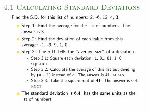
4.1 Calculating Standard Deviations

Find the S.D. for this list of numbers: 2, -6, 12, 4, 3.

Step 1: Find the average for the list of numbers. Theanswer is 3.

Step 2: Find the deviation of each value from thisaverage: -1, -9, 9, 1, 0.

Step 3: The S.D. tells the “average size” of a deviation.I Step 3.1: Square each deviation: 1, 81, 81, 1, 0.

squareI Step 3.2: Calculate the average of this list but dividing

by (n − 1) instead of n: The answer is 41. meanI Step 3.3: Take the square-root of 41. The answer is 6.4.

root

The standard deviation is 6.4. has the same units as thelist of numbers

4.2 Interpreting Standard Deviations

The standard deviation (S.D.) says how far numbers on a listare from their average (or mean). A majority (about 50% ormore) of entries will be somewhere around one S.D. from theaverage. Very few will be more than two or three S.D.s away.

AveAve- 1 S.D Ave+ 1 S.D.

Majority of observations

AveAve-2 S.D.s Ave+ 2 S.D.s

Almost all the observations

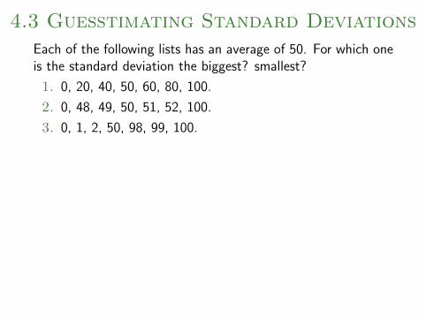
4.3 Guesstimating Standard Deviations

Each of the following lists has an average of 50. For which oneis the standard deviation the biggest? smallest?

1. 0, 20, 40, 50, 60, 80, 100.

2. 0, 48, 49, 50, 51, 52, 100.

3. 0, 1, 2, 50, 98, 99, 100.

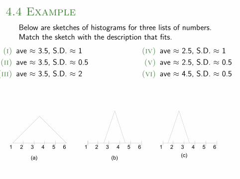
4.4 Example

Below are sketches of histograms for three lists of numbers.Match the sketch with the description that fits.

(i) ave ≈ 3.5, S.D. ≈ 1

(ii) ave ≈ 3.5, S.D. ≈ 0.5

(iii) ave ≈ 3.5, S.D. ≈ 2

(iv) ave ≈ 2.5, S.D. ≈ 1

(v) ave ≈ 2.5, S.D. ≈ 0.5

(vi) ave ≈ 4.5, S.D. ≈ 0.5

1 2 3 4 5 6 1 2 3 4 5 6 1 2 3 4 5 6

(a) (b) (c)

4.5 Example

Household size in the U.S. has a mean of 2.5 peopleapproximately. Which of these numbers would be a goodguess for the standard deviation? 0.14, 1.4 or 2?

4.6 Example

The Public Health Service found that for boys age 11 inHANES2, the average height was 146 cm and the SD was 8cm.

1. One boy was 170cm tall. He was above average bySDs.

2. If a boy was within 2 SDs of average height, the shortesthe could have been is cm and the tallest is cm.

3. Here are the heights of 3 boys: 150cm, 130 cm and165cm. Match the heights with the descriptions. Adescription may be used twice.

unusually short about average unusually tall

4.7 A Quick and Dirty Calculation

Consider a list with only two different numbers, a big oneand a small one. (Each number can be repeated manytimes).

In this case, the S.D. can be estimated using:

(bignumber

− smallnumber

)×√

fraction withbig number

× fraction withsmall number

.

Find the S.D. of the list of numbers: 1, -2, -2.

Find the S.D. of the list of numbers: -1, -1, -1, 1.

Can you use the short cut to calculate the standarddeviation of the list: 1, 2, 3, 4?

4.8 A Summary

To report the average and standard deviation, use thefollowing language:

In our data, the variable name here tends to bearound average here, give or takestandard deviation here.

AdviceUse means and standard deviations to summarize distributionsthat are roughly symmetric and with no outliers. Use the fivenumber summary otherwise.