Derivatives and Risk Management in Energy Markets

MØA-210Bård Misund

Professor of Finance

111

Social Media: LinkedIn, Google Scholar, Twitter, YouTube, Vimeo, FacebookEmployee Pages: UiS (Nor), UiS (Eng), NORCE1, NORCE2Personal Webpages: bardmisund.com, bardmisund.no, UiSResearch: Researchgate, IdeasRePEc, Publons, Orcid, SSRN, Others: Encyclopedia, Cristin1, Cristin2, Brage UiS, Brage USN, Nofima, FFI, SNF, HHUiS WP, Risk NetOp-Eds: Nationen, Fiskeribladet, Nordnorsk Debatt

About the author

Agenda

• Real and financial options in energy markets

• Crude oil– Locational arbitrage– Time arbitrage

• Natural gas– Time arbitrage– Locational spread (LNG, piped gas)– Price arbitrage

• Power– Spark spread

REAL OPTIONS IN THEENERGY INDUSTRY

What is a real option?

• Related to projects

• Investments in Property, buildings, factories and equipment

• Very often there are optionality/flexibility embedded in investmentdecisions

• Very important to identity the flexibility that is embedded in an investment opportunity

• Will increase the value of the project (>0)

Financial vs Real options

• Financial options (financial instruments)– Options on stocks, bonds, commodities, etc..– Traded options

• Real options (projects)– Non-traded options– Embedded options– Most investment projects contain some type of flexibility

(optionality)– Hidden uncertainty– These options can increase the value of a project– Often ignored or valued wrongly– Flexibility has a positive nonzero value that should be

quantified

Flexibility: example

• A company is considering building a new factory for producing a new product. The company has the possibility to terminate the project if it turns out not to be profitable. The company also has the possibility to expand the factory if things turn out better than expected.

Flexibility: example

• A company is considering building a new factory for producing a new product. The company has the possibility to terminate the project if it turns out not to be profitable. The company also has the possibility to expand the factory if things turn out better than expected.

• ” possibility to terminate the project” => optionality

• ” possibility to expand ” => optionality

Types of real options

• Abandonment options• Expansion options• Contraction options• Options to defer• Options to extend

Abandonment options

• This is an option to sell or terminate a project• An american option on the value of the project• The strike price of the option is the liquidation

value for the project minus termination costs

• An abandonment option counteracts the effect of extremely adverse outcomes and increases the value of the option as a whole

Expansion options

• This is an option to do additional investments and increase production once it is profitable to do so

• This is an american option on the value of increased capacity

• The strike price is the cost of increasing the capacity discounted to the exercise date

• The strike price is often dependent on the original investment– Overinvestment => reduced strike price

Contraction options

• This is an option to reduce the size of the operation of the project

• It is an american option on the value of lost capacity

• The strike price is the present value of future saved cash flows, discounted to the exercise date

Options to defer

• One of the most important options a company has is the option to defer a project

• This is an american option on the value of the project

Option to extend

• It is often possible to extend the life time of an asset by paying a fixed sum

• This is a European option on the asset’s future value

Options in the upstream oil and gas business

• The oil industry is characterised by large and long term projects

• Investments in billions dollars• Demanding technology• Investment decisions based on imperfact, little

and uncertain information• Long time horizon (>30 years)• Long lead times (time from the first investment is

carried out to the project generates a positive cash flow)

• Uncertain cash inflow (volatile oil prices)

Options in the upstream oil and gas business

• What can oil and gas companies do to improve the NPV’s of oil and gas projects?

Valuation approach – Decision trees

Uncertainty node

Decisionnode

Real options in downstream energy markets

• In energy markets (unlike financial markets) spread options and other correlation products are very important

• Majority of generation assets can be seen as complex versions of spread options

Real options vs standard NPV analysis

• The traditional approach to valuing an investment project is the net present value method (NPV)

• The NPV of a project is the present value of the incremental cash flow

• The discount rate used to calculate the NPV is a risk adjusted cost of capital, and is selected so that it reflects the risk of the project

Example

• An investment costs 100 MNOK and will last for 5 years

• The expected income from the investment is 25 MNOK per year

• The risk adjusted discount rate is 12%

• The NPV for this cash flow is:

Example

• The negative NPV is an indication that the project will reduce the value of the company from the perspective of the shareholders, and should not be carried out

• A positive NPV project should be initiated since it will increase the value of the company

The value of flexibility

• A problem with the traditional NPV approach is that many projects include options/optionality

• If a project includes one or more forms for flexibility, this is an indication that options are present

• An option value is always positive

• Flexibility therefore has a value/price that needs to be valued

Example: including the value of flexibility

• We can invest in a machine that costs 10 MUSD and can produce 1 product per year for ever

• Each product costs 0.90 MUSD to produce• The price for the product is 0.55 next year, and

increases with 4% per year after that• The risk free interest rate is 5% per year• We can invest in the machine at any time• There is no uncertainty

• What is the most amount of money you are willing to pay for the rights to this project?

Static NPV

• First we examine if it is profitable to invest today:

Static NPV

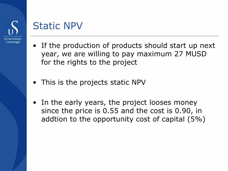
• If the production of products should start up next year, we are willing to pay maximum 27 MUSD for the rights to the project

• This is the projects static NPV

• In the early years, the project looses money since the price is 0.55 and the cost is 0.90, in addtion to the opportunity cost of capital (5%)

Static NPV

• If could therefore be profitable to wait with the start-up of the project, e.g. delay the investment with 5 years. The static NPV is then

• This analysis shows that is better to wait for 5 years instead of investing today

• But how to do this under uncertainty?

Investment under uncertainty

• If we also include the uncertainty in the project’s cash flow, the value of the implied put option will also affect the decision to delay the project

• We will use binomial trees to value the option

• We treat the option as an american option

• We pay the investment cost (=strike price) in order to receive an asset (the npv of future cash flows)

A simple NPV problem

• An analyst is evaluating a project which will geenrate a simple cash flows, X, arriving at time T

• The project’s return, volatility or covariance with the stock market is not directly observable

• The analyst must make some assumptions and simplifications, e.g. look at companies with comparable characteristics (e.g. to calculate the project beta)

A simple NPV problem

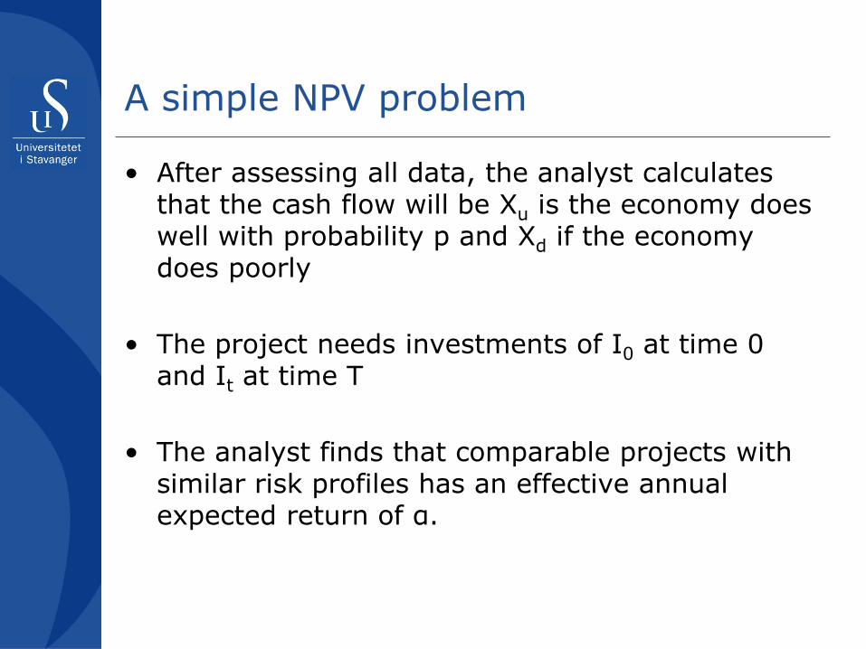
• After assessing all data, the analyst calculates that the cash flow will be Xu is the economy does well with probability p and Xd if the economy does poorly

• The project needs investments of I0 at time 0 and It at time T

• The analyst finds that comparable projects with similar risk profiles has an effective annual expected return of α.

A simple NPV problem

• The value of the project, V is then:

• If the choice is to invest today or never, we will invest in the project if:

Example

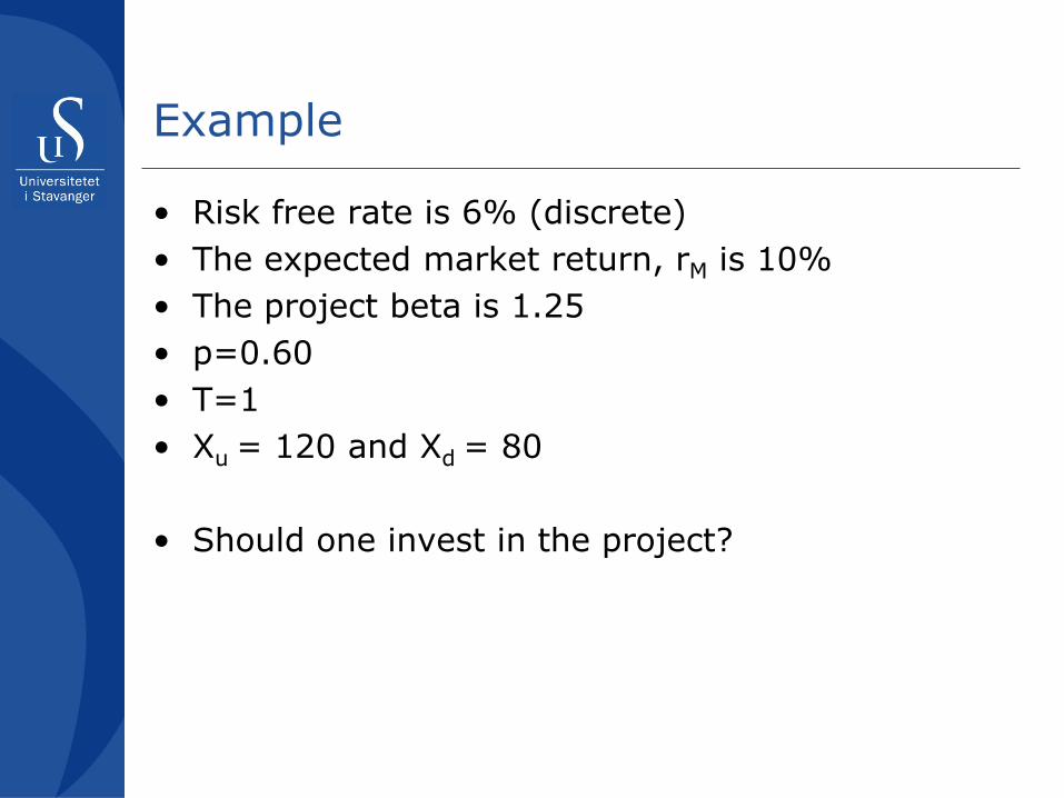
• Risk free rate is 6% (discrete)• The expected market return, rM is 10%• The project beta is 1.25• p=0.60• T=1• Xu = 120 and Xd = 80

• Should one invest in the project?

Example

• First, we calculate the expected return on the project:

• The expected cash flow is:

• The NPV of the project’s cash flows is:

Example

• If I0 = 10 and It is 95, the NPV for the project is

• If we instead assume that the investment at time T, It has some optionaliy, we can try to assess the optionality embedded in the project

Valuing the real options

• To calculate the option value we use binomial trees and risk neutral probabilities (risk neutral valuation)

• We can calculate the risk neutral probabilities for the project with the help of the forward price. Remember that the expected risk neutral price is equal to the forward price

• We have calculated V as the price of an asset that pays a simple cash flow at time T

Valuing the real options

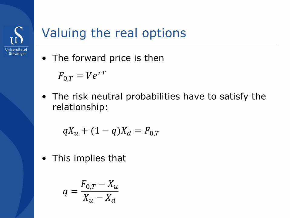
• The forward price is then

• The risk neutral probabilities have to satisfy the relationship:

• This implies that

Valuing the real options

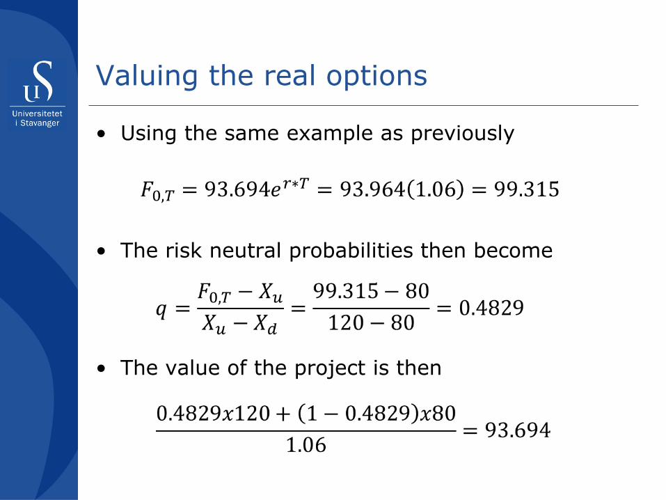
• Using the same example as previously

• The risk neutral probabilities then become

• The value of the project is then

Valuing the real options

• We can now try to calculate the value of the project given that we have a right, but not an obligation to invest at time T

q

1-q

-I0

max(Xu-IT, 0)

max(Xd-IT, 0)

Valuing the real options

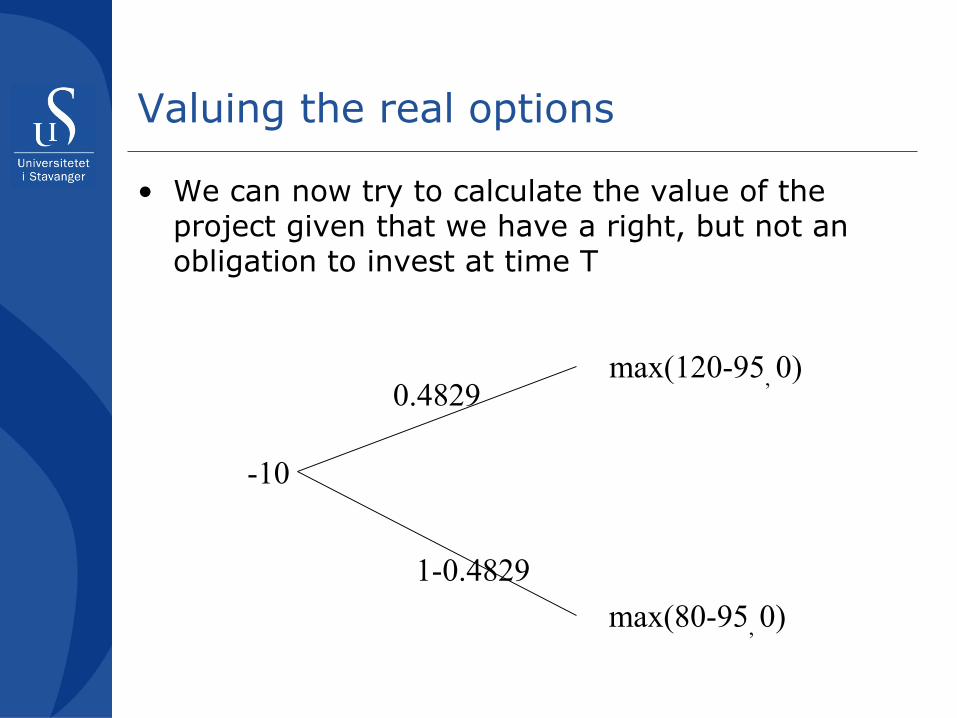
• We can now try to calculate the value of the project given that we have a right, but not an obligation to invest at time T

0.4829

1-0.4829

-10

max(120-95, 0)

max(80-95, 0)

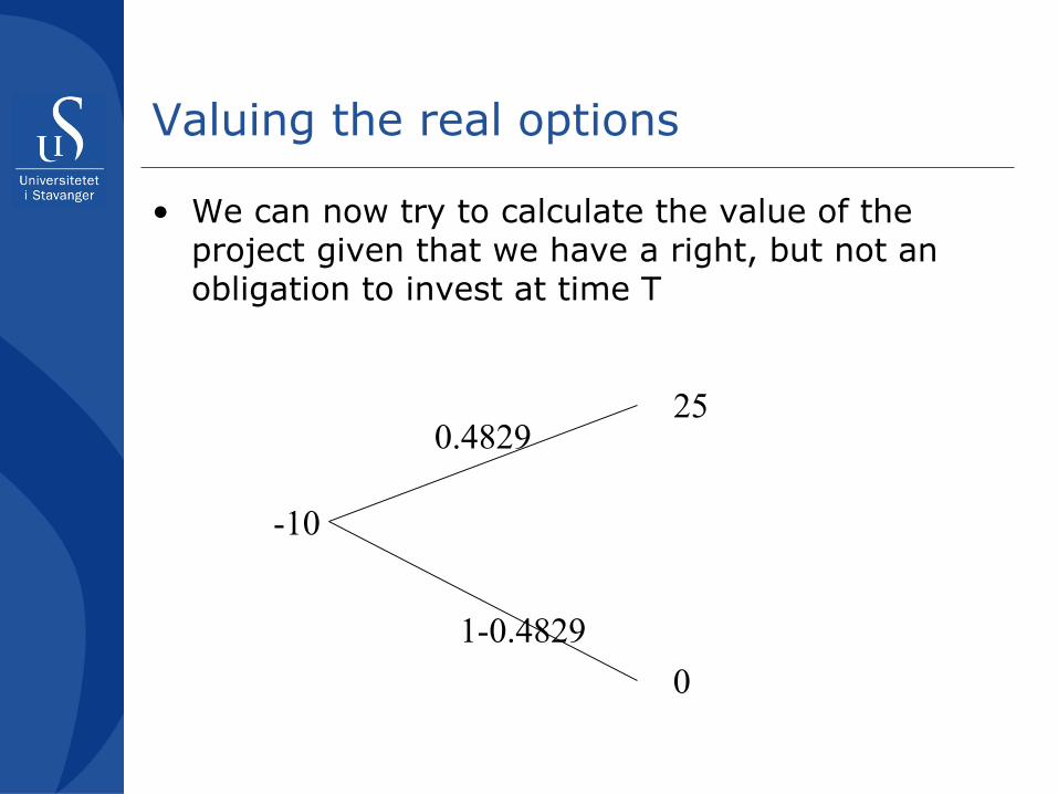
Valuing the real options

• We can now try to calculate the value of the project given that we have a right, but not an obligation to invest at time T

0.4829

1-0.4829

-10

25

0

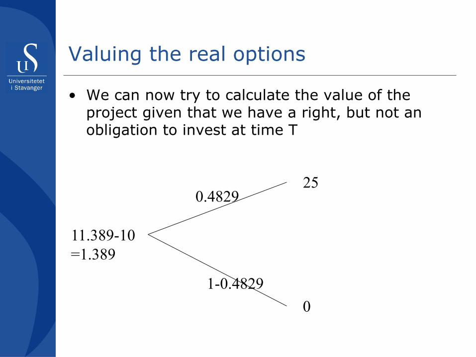
Valuing the real options

• We can now try to calculate the value of the project given that we have a right, but not an obligation to invest at time T

0.4829

1-0.4829

11.389-10=1.389

25

0

Valuation

• If we have risk neutral probabilities and the distribution of the cash flows we can value projects with options and non-linear cash flows

• When we value the options on stocks half the job is already done! The market has valued a present value of the company (=the underlying asset) for us (the market value)

• But when we value options on projects we need to calculate the present value of the project (=the underlying asset)ourselves since this cannot be observed (not market price)

Another example (2-year investment horizon)

• We will now examine when to invest in a risky project

• Equal to an american option: we pay the investment cost (strike) and receive the asset (the present value of the future cash flows)

• The project costs 100 MUSD and generates a perpetual cash flow, 1 year after the investment

• The expect cash flow the first year is 18 MUSD and is expected to grow by 3% per year

• The risk free rate is 7%, the market’s risk premium is 6% and the beta is 1.33

Another example (2-year investment horizon)

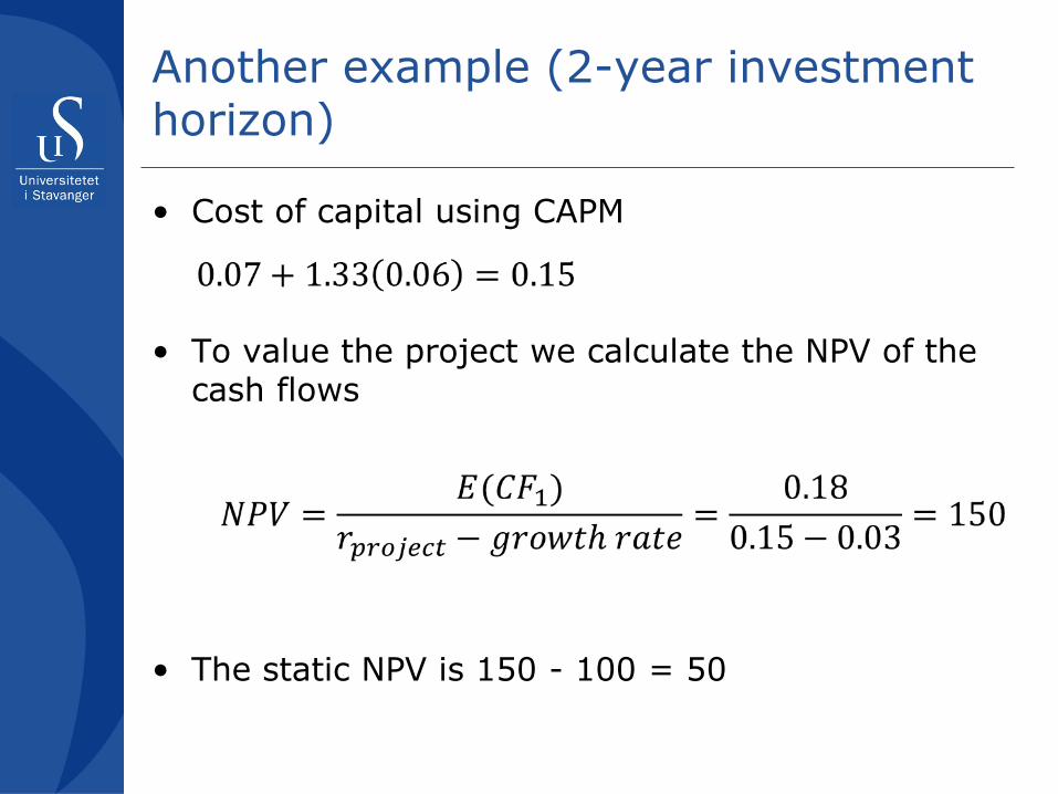
• Cost of capital using CAPM

• To value the project we calculate the NPV of the cash flows

• The static NPV is 150 - 100 = 50

Another example (2-year investment horizon)

• If we assume that we over the coming 2 years have the possibility to decide if we shall accept the project (invest or loose the investment opportunity)

• We need to assess the of waiting

Another example (2-year investment horizon)

• An important question is:

• What is the volatility of the project?• We assume that the volatility is 50%

• We can then use the Cox-Ross-Rubinstein approach to calculate u and d (2-step tree)

Another example (2-year investment horizon)

• Since the cash flows are lognormally distributed with 50% stdev, and the project value is proportional with the cash flows, the value of the project also be lognormally distributed with stdev 50%

150

247.3

91.0

407.7

150

55.2

Another example (2-year investment horizon)

• Since replication of real options is not possible (in the same way as is possible for financial options) the prices are not arbitrage free (ref. principle of no arbitrage)

• Hence, the values are not arbitrage free, but rather fair value estimates

Another example (2-year investment horizon)

• Valuing the option

• The inputs are:– The project’s initial present value, S0=150– The investment cost, X=100– The risk free rate (continuous), r = ln(1.07) =

6.6766%– Volatility, σ = 0.50– Time to maturity, T=2– The dividend is 18/150 (receive cash flow 18 in 1

year given investment), constant. Continuous dividend rate is ln (1.12) = 0.1133

Another example (2-year investment horizon)

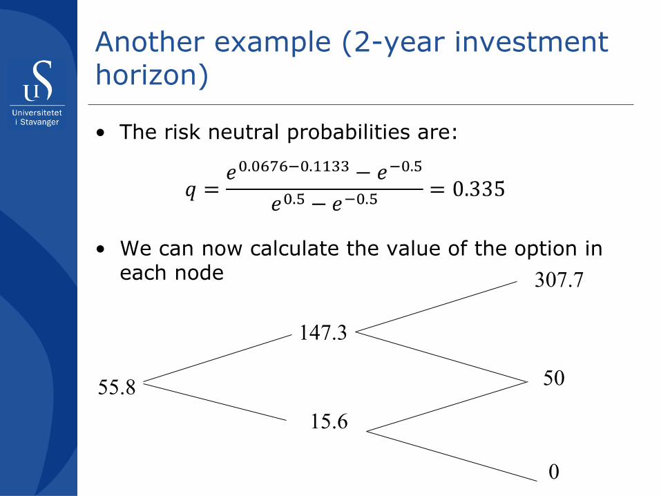
• The risk neutral probabilities are:

• We can now calculate the value of the option in each node

55.8

147.3

15.6

307.7

50

0

Another example (2-year investment horizon)

• The value of the project including the option is 55.8, which is higher than the static value of 50

• The value of the option to postpone the project 2 years is 55.8 – 50 = 5.8 MUSD

Relevant literature• Brooks, C., Prokopczuk, M. and Y. Wu (2013). Commodity futures prices: More evidence on forecast power, risk premia and the theory

of storage. The Quarterly Review of Economics and Finance 53, 73-85.• Brennan, M. (1958). The supply of storage. American Economic Review, 48(1), 50–72.• Brennan, M., & Schwartz, E. (1985). Evaluating natural resource investments. Journal of Business, 58, 135–157.• Fama, E., & French, K. (1987). Commodity futures prices: Some evidence on forecast power, premiums, and the theory of storage.

Journal of Business, 60(1), 55–73.• Pindyck, R. (2001). The dynamics of commodity spot and futures markets: A primer. Energy Journal, 22(3), 1–30.• Asche, F., Misund, B. and A. Oglend (2018). The case and cause of salmon price volatility. Marine Resource Economics 34(1), 23-38.• Misund, B. and R. Nygård (2018). Big Fish: Valuation of the world’s largest salmon farming companies. Marine Resource Economics

33(3), 245-261.• Misund, B. (2018). Volatilitet i laksemarkedet. Samfunnsøkonomen 2:41-54.• Misund, B. (2018). Common and fundamental risk factors in shareholder returns of Norwegian salmon producing companies.• Misund, B. (2018). Valuation of salmon farming companies. Aquaculture Economics & Management 22(1), 94-111.• Misund, B. & A. Oglend (2016). Supply and demand determinants of natural gas price volatility in the U.K.: A vector autoregression

approach. Energy 111, 178-189.• Asche, F., Misund, B. & A. Oglend (2016). Determinants of the futures risk premium in Atlantic salmon markets. Journal of Commodity

Markets, 2(1), 6-17.• Misund, B. & F. Asche (2016). Hedging efficiency of Atlantic salmon futures. Aquaculture Economics & Management 20(4), 368-381.• Asche, F., Misund, B. & A. Oglend (2016). The spot-forward relationship in Atlantic salmon markets. Aquaculture Economics &

Management 20(2), 222-234. • Asche, F., Misund, B. and A. Oglend (2016). Fish Pool Priser – Hva Forteller de oss om fremtidige laksepriser? Norsk Fiskeoppdrett nr.8

2016, p.74-77.• Symeonidis, L., Prokopczuk, M. Brooks, C. and E. Lazar (2012). Futures basis, inventory and commodity price volatility: An empirical

analysis. Economic Modelling 29, 2651-2663.

50