DERIVATIVESDERIVATIVES

3

3.9Linear Approximations

and Differentials

In this section, we will learn about:

Linear approximations and differentials

and their applications.

DERIVATIVES

The idea is that we use the tangent line at

(a, f(a)) as an approximation to the curve

y = f(x) when x is near a.

An equation of this tangent line is y = f(a) + f’(a)(x - a)

LINEAR APPROXIMATIONS

Figure 3.9.1, p. 189

The approximation

f(x) ≈ f(a) + f’(a)(x – a)

is called the linear approximation

or tangent line approximation of f at a.

Equation 1LINEAR APPROXIMATION

The linear function whose graph is

this tangent line, that is,

L(x) = f(a) + f’(a)(x – a)

is called the linearization of f at a.

Equation 2LINEARIZATION

Find the linearization of the function

at a = 1 and use it to

approximate the numbers

Are these approximations overestimates or

underestimates?

( ) 3f x x 3.98 and 4.05

Example 1LINEAR APPROXIMATIONS

The derivative of f(x) = (x + 3)1/2 is:

So, we have f(1) = 2 and f’(1) = ¼.

1/ 212

1'( ) ( 3)

2 3f x x

x

Example 1Solution:

Putting these values into Equation 2,

we see that the linearization is:

14

( ) (1) '(1)( 1)

2 ( 1)

7

4 4

L x f f x

x

x

Example 1Solution:

The corresponding linear approximation is:

(when x is near 1)

In particular, we have:

and

7 0.983.98 1.995

4 47 1.05

4.05 2.01254 4

73

4 4

xx

Example 1Solution:

We see that:

The tangent line approximation is a good

approximation to the given function when x is near 1.

Our approximations are overestimates, because

the tangent line lies

above the curve.

Example 1

Figure 3.9.2, p. 190

Solution:

Of course, a calculator could give us

approximations for

we can compare the estimates from the linear

approximation in Example 1 with the true

values.

3.98 and 4.05

Example 1LINEAR APPROXIMATIONS

Look at the table

and the figure.

The tangent line

approximation gives goodestimates if x is close to 1.

However, the accuracy decreases when x is farther away from 1.

LINEAR APPROXIMATIONS

Figure 3.9.2, p. 190

For what values of x is the linear

approximation accurate

to within 0.5?

What about accuracy to within 0.1?

73

4 4

xx

Example 2LINEAR APPROXIMATIONS

Accuracy to within 0.5 means that

the functions should differ by less than 0.5:

73 0.5

4 4

xx

Example 2Solution:

Equivalently, we could write:

This says that the linear approximation should lie between the curves obtained by shifting the curve

upward and downward by an amount 0.5

73 0.5 3 0.5

4 4

xx x

3y x

Example 2Solution:

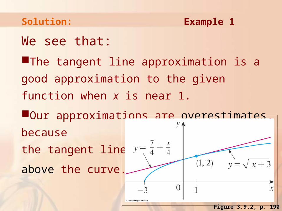
The figure shows the tangent line

intersecting the upper

curve at P

and Q.

(7 ) / 4y x 3 0.5y x

Example 2

Figure 3.9.3, p. 191

Solution:

Thus, we see from the graph

that the approximation

is accurate to within 0.5 when

-2.6 < x < 8.6

We have roundedto be safe.

73

4 4

xx

Example 2

Figure 3.9.3, p. 191

Solution:

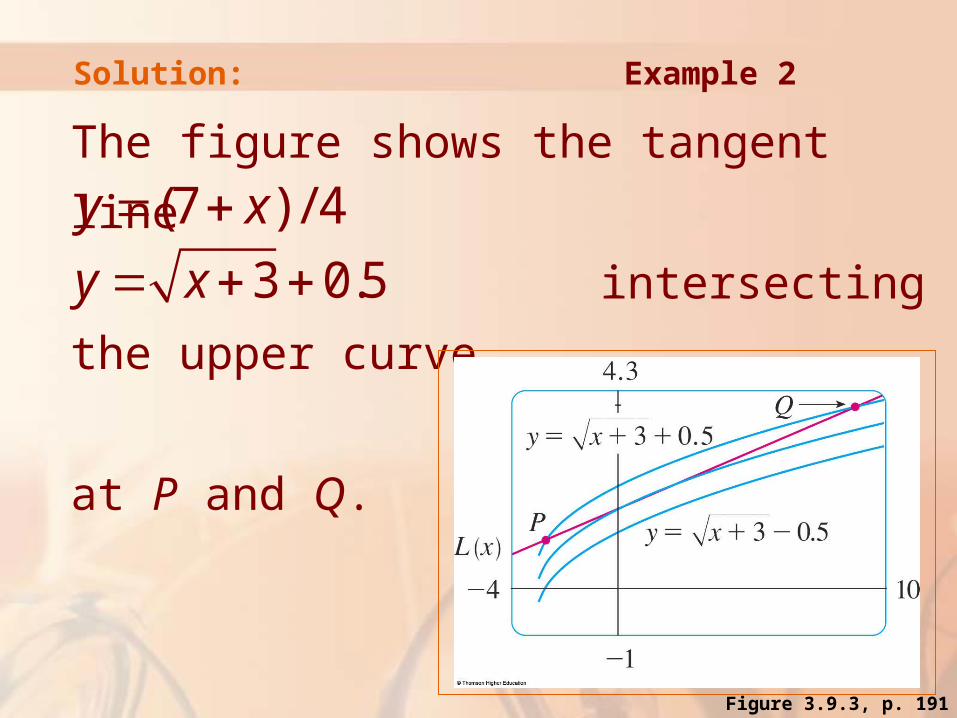
Similarly, from this figure, we see that

the approximation is accurate to within 0.1

when -1.1 < x < 3.9

Example 2

Figure 3.9.4, p. 191

Solution:

Linear approximations are often used

in physics.

In analyzing the consequences of an equation, a physicist sometimes needs to simplify a function by replacing it with its linear approximation.

APPLICATIONS TO PHYSICS

For instance, in deriving a formula for

the period of a pendulum, physics textbooks

obtain the expression aT = -g sin θ for

tangential acceleration.

Then, they replace sin θ by θ with the remark

that sin θ is very close to θ if θ is not too large.

APPLICATIONS TO PHYSICS

You can verify that the linearization of

the function f(x) = sin x at a = 0 is L(x) = x.

So, the linear approximation at 0 is:

sin x ≈ x

APPLICATIONS TO PHYSICS

The ideas behind linear approximations

are sometimes formulated in the

terminology and notation of differentials.

DIFFERENTIALS

If y = f(x), where f is a differentiable

function, then the differential dx

is an independent variable.

That is, dx can be given the value of any real number.

DIFFERENTIALS

The differential dy is then defined in terms

of dx by the equation

dy = f’(x)dx

So, dy is a dependent variable—it depends on the values of x and dx.

If dx is given a specific value and x is taken to be some specific number in the domain of f, then the numerical value of dy is determined.

Equation 3DIFFERENTIALS

The geometric meaning of differentials

is shown here.

Let P(x, f(x)) and Q(x + ∆x, f(x + ∆x)) be points on the graph of f.

Let dx = ∆x.

DIFFERENTIALS

Figure 3.9.5, p. 192

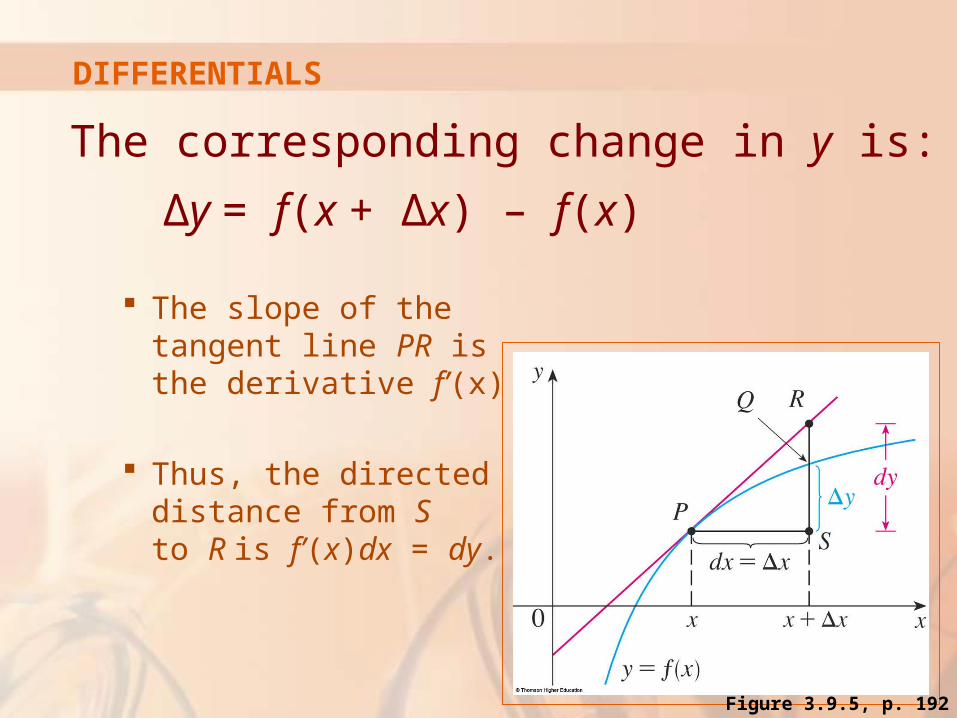
The corresponding change in y is:

∆y = f(x + ∆x) – f(x)

The slope of the tangent line PR is the derivative f’(x).

Thus, the directed distance from S to R is f’(x)dx = dy.

DIFFERENTIALS

Figure 3.9.5, p. 192

Therefore, dy represents the amount that the tangent line

rises or falls (the change in the linearization).

∆y represents the amount

that the curve y = f(x)

rises or falls when x

changes by an amount dx.

DIFFERENTIALS

Figure 3.9.5, p. 192

Compare the values of ∆y and dy

if y = f(x) = x3 + x2 – 2x + 1

and x changes from:

a. 2 to 2.05

b. 2 to 2.01

Example 3DIFFERENTIALS

Figure 3.9.6, p. 192

We have:

f(2) = 23 + 22 – 2(2) + 1 = 9

f(2.05) = (2.05)3 + (2.05)2 – 2(2.05) + 1

= 9.717625

∆y = f(2.05) – f(2) = 0.717625

Example 3 aSolution:

In general,

dy = f’(x)dx = (3x2 + 2x – 2) dx

When x = 2 and dx = ∆x = 0.05,

this becomes:

dy = [3(2)2 + 2(2) – 2]0.05

= 0.7

Example 3 aSolution:

We have:

f(2.01) = (2.01)3 + (2.01)2 – 2(2.01) + 1

= 9.140701

∆y = f(2.01) – f(2) = 0.140701

When dx = ∆x = 0.01,

dy = [3(2)2 + 2(2) – 2]0.01 = 0.14

Example 3 bSolution:

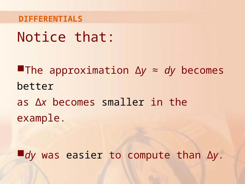
Notice that:

The approximation ∆y ≈ dy becomes better

as ∆x becomes smaller in the example.

dy was easier to compute than ∆y.

DIFFERENTIALS

In the notation of differentials,

the linear approximation can be

written as:

f(a + dx) ≈ f(a) + dy

DIFFERENTIALS

For instance, for the function

in Example 1, we have:

( ) 3f x x

'( )

2 3

dy f x dx

dx

x

DIFFERENTIALS

If a = 1 and dx = ∆x = 0.05, then

and

This is just as we found in Example 1.

0.050.0125

2 1 3dy

4.05 (1.05) (1) 2.0125f f dy

DIFFERENTIALS

The radius of a sphere was measured

and found to be 21 cm with a possible error

in measurement of at most 0.05 cm.

What is the maximum error in using this

value of the radius to compute the volume

of the sphere?

Example 4DIFFERENTIALS

If the radius of the sphere is r, then

its volume is V = 4/3πr3.

If the error in the measured value of r is denoted by dr = ∆r, then the corresponding error in the calculated value of V is ∆V.

Example 4Solution:

This can be approximated by the differential

dV = 4πr2dr

When r = 21 and dr = 0.05, this becomes:

dV = 4π(21)2 0.05 ≈ 277

The maximum error in the calculated volume is about 277 cm3.

Example 4DIFFERENTIALS

Relative error is computed by dividing

the error by the total volume:

Thus, the relative error in the volume is about three times the relative error in the radius.

2

343

43

V dV r dr dr

V V r r

RELATIVE ERROR Note

In the example, the relative error in the radius

is approximately dr/r = 0.05/21 ≈ 0.0024

and it produces a relative error of about 0.007

in the volume.

The errors could also be expressed as percentage errors of 0.24% in the radius and 0.7% in the volume.

NoteRELATIVE ERROR