DEPTH-INTEGRATED, NON-HYDROSTATIC MODEL …nsgl.gso.uri.edu/hawau/hawauy10003.pdf ·...
107
DEPTH-INTEGRATED, NON-HYDROSTATIC MODEL WITH GRID NESTING FOR TSUNAMI GENERATION, PROPAGATION, AND RUNUP A DISSERTATION SUBMITTED TO THE GRADUATE DIVISION OF THE UNIVERSITY OF HAWAI`I AT MĀNOA IN PARTIAL FULFILLMENT OF THE REQUIREMENTS FOR THE DEGREE OF DOCTOR OF PHILOSOPHY IN OCEAN AND RESOURCES ENGINEERING AUGUST 2010 By Yoshiki Yamazaki Dissertation Committee: Kwok Fai Cheung, Chair Gerard J. Fryer Geno Pawlak Ian N. Robertson John C. Wiltshire
Transcript of DEPTH-INTEGRATED, NON-HYDROSTATIC MODEL …nsgl.gso.uri.edu/hawau/hawauy10003.pdf ·...

DEPTH-INTEGRATED, NON-HYDROSTATIC MODEL WITH GRID NESTING FOR TSUNAMI GENERATION, PROPAGATION, AND RUNUP
A DISSERTATION SUBMITTED TO THE GRADUATE DIVISION OF THE UNIVERSITY OF HAWAI`I AT MĀNOA IN PARTIAL FULFILLMENT OF THE
REQUIREMENTS FOR THE DEGREE OF
DOCTOR OF PHILOSOPHY
IN
OCEAN AND RESOURCES ENGINEERING
AUGUST 2010
By
Yoshiki Yamazaki
Dissertation Committee:
Kwok Fai Cheung, Chair Gerard J. Fryer Geno Pawlak
Ian N. Robertson John C. Wiltshire

ii
We certify that we have read this dissertation and that, in our opinion, it is satisfactory in
scope and quality as a dissertation for the degree of Doctor of Philosophy in Ocean and
Resources Engineering.
DISSERTATION COMMITTEE
_________________________________ Chairperson
_________________________________
_________________________________
_________________________________
_________________________________

iii
Copyright © 2010
by
Yoshiki Yamazaki

iv
ACKNOWLEDGEMENTS
I would like to express my deepest appreciation to my advisor Prof. Kwok Fai Cheung
for his guidance, support, and encouragement throughout my graduate studies at the
University of Hawaii. He is the one, who opened the door for my career in ocean
engineering and science, and led and guided me in the very best direction to achieve my
goal. The knowledge and experience I gained from him are valuable and unforgettable.
My special thanks go to my dissertation committee: Dr. Gerard Fryer for his
encouragement and valuable comments on seismological processes associated with
tsunami generation, Prof. Geno Pawlak for providing insights regarding wave dispersion
and seafloor displacement, Prof. Ian Robertson for valuable comments on applications of
tsunami modeling in structural engineering, and Dr. John Wiltshire for his
encouragement and valuable input on geological processes of tropical islands related to
tsunami studies.
I would like to express my warmest and special thanks to George Curtis sensei of the
University of Hawaii at Hilo, who always supported and looked after me during my study
in Hawaii; Prof. Zygmunt Kowalik of the University of Alaska, Fairbanks, who taught
me from the very basics of numerical modeling and provided continuous support through
the model development; and Prof. Chen-Jun Yang of Shanghai Jiao Tong University,
who helped me achieve deep understanding of water wave mechanics. I also would like
to thank Prof. Juan Horrillo, Mr. William Knight, and Prof. Tokihiro Katsui, who kindly
helped me gain my knowledge on numerical modeling. I would like to thank Dr. Darren
Okimoto, who supported me through the University of Hawaii Sea Grant College
Program. Thanks also go to Ms. Edith Katada and Ms. Natalie Nagai, who kindly took
care of the administrative paperwork for me.

v
I would like to thank Prof. Guus Stelling and Dr. Marcelo Zijlema for their valuable input
on the momentum-conserved advection scheme, Dr. Michael Briggs for providing the
recorded data of the conical island experiment, Dr. Masafumi Matsuyama for providing
the input and recorded data of the Monai Valley experiment, Dr. Gavin Hayes for
supplying his latest finite fault solution for the 2009 Samoa Earthquake, and Prof.
Hermann Fritz and Prof. Shunichi Koshimura for providing the recorded runup and
inundation data for the 2009 Samoa Tsunami around Tutuila. I also would like to thank
all those who have helped me achieve in-depth understanding of tsunamis including but
not limited to Prof. Nobuo Shuto, Prof. Charles Mader, Prof. Yoshimitsu Okada, Prof.
Kenji Satake, Prof. Fumihiko Imamura, Prof. Harry Yeh, Dr. Harold Mofjeld, Dr. Vasily
Titov, and Dr. Tatsuo Kuwayama,
My special thanks go to all those who studied and had fun with me for these years, Dr.
Yong Wei, Mr. Volker Roeber, Mr. Alex Sánchez, Ms. Sophie Munger, Ms. Megan Craw,
Mr. Pablo Duarte-Quiroga, Mr. Jacob Tyler, Mr. Yefei Bai, Dr. Liujuan Tang, Dr. Ning
Li, Dr. Jinfeng Zhang, Dr. Xiuying Kang, Mr. Shailesh Namekar, Mr. Justin Goo, Ms.
Shi Shu, Mr. Lei Yan, Dr. Krishnakumar Rajagopalan, Mr. Richard Carter, Mr. Jinghai
Yang, Mr. Suvabrata Das, Mr. Masoud Hayatdavoodi, Mr. Justin Stopa, Mr. Troy
Heitmann, Dr. Liang Ge, Mr. Long Chen, Dr. Yongyan Wu, Dr. Yohei Shinozuka, Mr.
Greg Francis, Mr. Vasco Nunes, Mr. Joji Uchiyama, Ms. Akiko Manabe, and Ms.
Michiyo Tomioka.
Finally, deepest and warmest thanks go to my parents Yoshishige and Haruyo Yamazaki
for their unconditional support and encouragement throughout my life, and to my family,
Yoshiyuki, Toshio, Hisako, Yoshihiko, Masanobu, Minako, Ikuya, and Timothy, who
always share happy moments with me. I dedicate this work to my grandmother, Chiyoko
Yamazaki, who always believes in me and waited for this day to come.
vi
This dissertation is funded by a grant/cooperative agreement from the National Oceanic
and Atmospheric Administration, Project R/IR-2, which is sponsored by the University of
Hawaii Sea Grant College Program, SOEST, under Institutional Grant No.
NA09OAR4170060 from NOAA Office of Sea Grant, Department of Commerce. The
National Tsunami Hazard Mitigation Program, Hawaii State Civil Defense, and Joint
Institute for Marine and Atmospheric Research provided additional support for this study.
UNIHI-SEAGRANT-XD-09-01.

vii
ABSTRACT
This dissertation describes the formulation, verification, and validation of a dispersive
wave model with a shock-capturing scheme, and its implementation for basin-wide
evolution and coastal runup of tsunamis using two-way nested computational grids. The
depth-integrated formulation builds on the nonlinear shallow-water equations and utilizes
a non-hydrostatic pressure term to describe weakly dispersive waves. The semi-implicit,
finite difference solution captures flow discontinuities associated with bores or hydraulic
jumps through a momentum conservation scheme, which also accounts for energy
dissipation in the wave breaking process without the use of an empirical model. An
upwind scheme extrapolates the free surface elevation instead of the flow depth to
provide the flux in the momentum and continuity equations. This eliminates depth
extrapolation errors and greatly improves the model stability, which is essential for
computation of energetic breaking waves and runup.
The vertical velocity term associated with non-hydrostatic pressure also describes
tsunami generation and transfer of kinetic energy due to dynamic seafloor deformation. A
depth-dependent Gaussian function smoothes bathymetric features smaller than the water
depth to improve convergence of the implicit, non-hydrostatic solution. A two-way grid-
nesting scheme utilizes the Dirichlet condition of the non-hydrostatic pressure and both
the velocity and surface elevation at the grid interface to ensure propagation of dispersive
waves and discontinuities through computational grids of different resolution. The inter-
grid boundary can adapt to topographic features to model wave transformation processes
at optimal resolution and computational efficiency.
The computed results show very good agreement with data from previous laboratory
experiments for wave propagation, transformation, breaking, and runup over a wide range

viii
of conditions. The present model is applied to the 2009 Samoa Tsunami for
demonstration and validation. These case studies confirm the validity and effectiveness of
the present modeling approach for tsunami research and impact assessment. Since the
numerical scheme to the momentum and continuity equations remains explicit, the
implicit non-hydrostatic solution is directly applicable to existing nonlinear shallow-
water models.

ix
TABLE OF CONTENTS
ACKNOWLEGEMENTS …………………………………………………………… iv
ABSTRACT ………………………………………………………………………..... vii
LIST OF TABLES …………………………………………………………………... xi
LIST OF FIGURES ………………………………………………………………..... xii
1. INTRODUCTION …………………………………………………………… 1
2. THEORETICAL FORMULATION ………………………………………… 6
2.1 Three-dimensional Governing Equations …………………………………. 6
2.2 Depth-integrated Governing Equations …………………………………… 9
2.3 Linear Dispersion Relation ……………………………………………… 15
3. NUMERICAL FORMULATION …………………………………………… 20
3.1 Hydrostatic Solution in Spherical Grids ………………………………… 21
3.2 Non-hydrostatic Solution in Spherical Grids ……………………………… 26
3.3 Solutions in Cartesian Grids ………………………………………………. 30
4. IMPLEMENTATION FOR TSUNAMI MODELING ……………………… 34
4.1 Wet-dry Moving Boundary Condition …………………………………… 34
4.2 Grid-nesting Scheme ………………………………………………………. 36
4.3 Depth-dependent Smoothing Scheme …………………………………… 39
4.4 NEOWAVE ……………………………………………………………… 41
5. DISPERSION AND NESTED GRIDS ……………………………………… 44
5.1 Solitary Wave Propagation in a Channel ………………………………… 44
5.2 Sinusoidal Wave Propagation over a Bar ………………………………… 48
5.3 N-wave Transformation and Runup ……………………………………… 50
6. WAVE BREAKING AND RUNUP …………………....................................... 56
6.1 Solitary Wave Runup on a Plane Beach ………………………………… 56
6.2 Solitary Wave Runup on a Conical Island ………………………………… 61

x
7. THE 2009 SAMOA TSUNAMI ………………………………………………. 68
7.1 Model Setup ……………………………………………………………… 68
7.2 Tsunami Generation ……………………………………………………… 71
7.3 Surface Elevation and Runup ……………………………………………… 75
8. CONCLUSIONS AND RECOMMENDATIONS ……………………………. 82
REFERENCES ……………………………………………………………………… 86

xi
LIST OF TABLES
Table Page
5.1 Recorded runup for the six trials from Matsuyama and Tanaka (2001) ………. 53

xii
LIST OF FIGURES
Figure Page
2.1 Schematic of the free-surface flow generated by seafloor deformation……….. 6
2.2 Linear dispersion relation……………………………………………………… 18
3.1 Definition sketch of spatial grid……………………………………………… 20
4.1 Schematic of a two-level nested grid system. (a) Nested-gird configuration. …
(b) Close-up view of the inter-grid boundary and data transfer protocol……... 37
4.2 Schematic of two-way grid-nesting and time-integration scheme……………... 38
4.3 Schematic of module structure of NEOWAVE……………………………… 42
5.1 Solitary wave profiles along a channel with constant water depth…………… 45
5.2 Propagation of solitary wave across two levels of nested grids in a channel
of constant depth. ……………………………………………………………. 47
5.3 Definition sketch of wave transformation over a submerged bar. …….
(a) Laboratory setup. (b) Numerical setup……………………………………... 48
5.4 Comparison of computed and measured free surface elevations over and
behind a submerged bar……………………………………………………… 49
5.5 Input data for Monai Valley experiment. (a) Level-1 computational domain.
(b) Initial wave profile…………………………………………….................. 52
5.6 Time series of surface elevation at gauges in Monai Valley experiment.
(a) Comparison of measurements with nested-grid solution. (b) Comparison of
nested and uniform grid solutions……………………………………………… 53
5.7 Runup and Inundation comparisons. (a) Runup. (b) Inundation………………. 54
6.1 Definition sketch of solitary wave runup on a plane beach……………………. 56
6.2 Surface profiles of solitary wave transformation on a 1:19.85 plane beach
with A/h = 0.3…………………………………………………………………... 58

xiii
6.3 Solitary wave runup on a plane beach as a function of incident wave height.
(a) 1/5.67 (Hall and Watts, 1953). (b) 1/15 (Li and Raichlen, 2002). ….
(c) 1/19.85 (Synolakis, 1987)…………………………….…………………… 60
6.4 Schematic sketch of the conical island experiment. (a) Perspective view. ..
(b) Side view (center cross section)……………………………………………. 61
6.5 Wave transformation in front of the conical island. (a) A/h = 0.045. (b) A/h
= 0.096. (c) A/h = 0.181………………………………………………………... 63
6.6 Wave transformation on the leeside of the conical island. (a) A/h = 0.045.
(b) A/h = 0.096. (c) A/h = 0.181……………………………………………… 64
6.7 Time series of surface elevations at gauges around a conical island. (a) A/h
= 0.045. (b) A/h = 0.096. (c) A/h = 0.181………………………………………. 66
6.8 Inundation and runup around a conical island. (a) A/h = 0.045. (b) A/h =
0.096. (c) A/h = 0.181………………………………………………………...... 67
7.1 Bathymetry and topography in the modeled region for the 2009 Samoa
Tsunami. (a) Level-1 computational domain. (b) Close-up view of rupture
configuration and Samoa Islands………………………………………………. 69
7.2 Coverage of levels 2, 3, and 4 computational domain. (a) Original
bathymetry and topography. (b) Smoothed data with depth-dependent
Gaussian function………………………………………………………………. 70
7.3 Schematic of planar fault model……………………………………………….. 72
7.4 Time sequence of rupture and tsunami generation. (a) Slip distribution. .
(b) Sea floor deformation. (c) Surface elevation………………………………. 74
7.5 Maximum surface elevation for the 2009 Samoa Tsunami……………………. 75
7.6 Wave propagation and inundation at inner Pago Pago Harbor………………… 76
7.7 Time series and spectra of surface elevations at water level stations………… 78

xiv
7.8 Detailed bathymetry and resonance modes around Pago Pago Harbor. .
(a) bathymetry. (b) First mode at 18 min. (c) Second mode at 11 min. .
(d) Third mode at 9.6 min……………………………………………………… 79
7.9 Runup and inundation at inner Pago Pago Harbor……………………………... 81

1
CHAPTER 1
INTRODUCTION
Tsunamis generated by earthquakes are typically modeled as shallow-water waves with a
spherical coordinate system for their propagation around the globe. The finite difference
method, owing to its simplicity in formulation and ease of implementation, is widely used
in the solution schemes of the depth-integrated governing equations. These explicit
schemes provide an efficient approach to describe the tsunami evolution process from
generation, propagation, to runup through a series of two-way nested grids (e.g., Liu et al.,
1995b; Goto et al., 1997; Titov and Synolakis, 1998; and Wei et al., 2008). Consistent
with the shallow-water approach, the initial tsunami wave assumes the vertical
component of the seafloor deformation due to earthquake rupture (Kajiura, 1970). This
static sea surface deformation simplifies the tsunami generation mechanism to provide a
practical method for reconstruction of real-field tsunamis. Recent studies, however,
suggest wave dispersion and breaking as well as dynamic seafloor deformation could
have non-negligible effects on the tsunami evolution and runup processes (Ohmachi et al.,
2001; Horrillo et al., 2006; Wei et al., 2006; and Song et al., 2008).
The commonly used finite difference schemes for the nonlinear shallow-water equations
are non-conservative leading to volume loss and energy dissipation as the wave steepness
increases and the flow approaches discontinuous. This turns out to be a crucial modeling
issue when tsunami bores develop nearshore and the results become grid-size dependent.
The finite volume method based on the conservative form of the nonlinear shallow-water
equations captures flow discontinuities and conserves flow volume through a Riemann
solver (e.g., Dodd, 1998; Zhou et al., 2001; Wei et al., 2006; Wu and Cheung, 2008; and
George, 2010). This approach approximates breaking waves as bores or hydraulic jumps
through conservation of momentum and accounts for energy dissipation across flow

2
discontinuities without the use of empirical relations. Stelling and Duinmeijer (2003)
developed an equivalent shock-capturing scheme for finite difference shallow-water
models. This momentum-conserved advection scheme, which is derived from the
conservative formulation of the momentum equations, produces comparable results as a
Riemann solver.
The nonlinear shallow-water equations are hydrostatic and are unable to describe wave
dispersion. Through a classical Boussinesq model, Horrillo et al. (2006) showed wave
dispersion in basin-wide tsunami propagation results in a sequence of trailing waves that
might have significant effects on coastal runup. Boussinesq-type models, however,
involve a complex equation system with high-order dispersive terms that might not be
amenable to the grid-nesting schemes commonly used in tsunami modeling. In contrast,
Casulli (1995) proposed an alternative approach to model dispersive waves that
decomposes the pressure into hydrostatic and non-hydrostatic components. The explicit
hydrostatic solution is determined first and then an implicit solution is obtained for wave
dispersion associated with the non-hydrostatic pressure. Researchers have implemented
this approach in the formulation of full three dimensional, multi-layer three-dimensional,
and depth-integrated two-dimensional models (e.g., Mahadevan et al., 1996a; Casulli and
Stelling, 1998; Stansby and Zhou, 1998; Stelling and Zijlema, 2003; and Walters, 2005).
The dispersive term is described with the first derivative of the non-hydrostatic pressure
in both three-dimensional and two-dimensional models. The depth-integrated governing
equations are relatively simple and analogous to the nonlinear shallow-water equations
with the addition of a vertical momentum equation and non-hydrostatic terms in the
horizontal momentum equations. The depth-integrated, non-hydrostatic models of
Stelling and Zijlema (2003) and Walters (2005) produce comparable or better results in
comparison to the classical Boussinesq equations.

3
Zijlema and Stelling (2008) presented a multi-layer, non-hydrostatic formulation with a
momentum conservation scheme for the advective terms and an upwind approximation in
the continuity equation, and derived semi-implicit schemes for both the hydrostatic and
non-hydrostatic solutions. Their two-layer model can handle wave breaking without the
use of empirical relations for energy dissipation and provide comparable results with
those of extended Boussinesq models (Nwogu, 1993; Madsen et al., 1997; Chen et al.,
2000; and Lynett et al., 2002). Such a non-hydrostatic approach, if builds on existing
nonlinear shallow-water models with explicit schemes (e.g., Shuto and Goto, 1978;
Mader and Curtis, 1991; Kowalik and Murty, 1993; Liu et al., 1995b; Imamura, 1996;
and Titov and Synolakis, 1998), will have greater application in the tsunami research
community. Numerical stability, however, is a critical issue. The difficulty lies in the flux
approximation, in which the velocity and flow depth are evaluated at different locations
in a finite difference scheme. The resulting errors in flux estimations often become the
source of instability. Mader (1988) proposed a unique upwind scheme that extrapolates
the surface elevation instead of the flow depth to determine explicitly the flux in the
continuity equation of a nonlinear shallow-water model. Kowalik et al. (2005)
implemented this upwind flux approximation in their nonlinear shallow-water model and
showed remarkable stability in simulating propagation and runup of the 2004 Indian
Ocean Tsunami on a global scale.
This dissertation integrates the experience from previous works and presents a depth-
integrated non-hydrostatic model capable of handling dispersion as well as flow
discontinuities associated with breaking waves and hydraulic jumps for tsunami modeling.
The formulation, which builds on an explicit scheme of the nonlinear shallow-water
equations, allows a direct implementation of the upwind flux approximation of Mader
(1988) to improve model stability for discontinuous flows. The first-order partial

4
differential equations facilitate the implementation of two-way nested computational
grids for simultaneous computation of basin-wide evolution and coastal runup of
tsunamis. The vertical velocity term associated with the non-hydrostatic pressure also
describes tsunami generation due to seafloor deformation. Recent advances in seismic
inverse algorithms such as Ji et al. (2002) and Honda et al. (2004) allow description of
rise time and rupture propagation over the source area, and provide the time series of
seafloor displacement as input to the non-hydrostatic model. However, dispersive models
based on non-hydrostatic or Boussinesq-type formulations are prone to instabilities
created by localized, steep bottom gradients (Horrillo et al., 2006; and Løvholt and
Perdersen, 2008). A depth-dependent Gaussian function is implemented to allow
smoothing of bathymetric features smaller than the water depth to improve convergence
of the implicit, non-hydrostatic solution.
In this dissertation, Chapter 2 describes the derivation of the depth-integrated non-
hydrostatic equations from the three-dimensional Navier-Stokes equations and the
continuity equation in the spherical coordinate system. Linearization of the governing
equations allows derivation of the dispersion relation for comparison with the exact linear
dispersion relation from Airy wave theory. Chapter 3 introduces the discretization
scheme and provides the numerical formulation for the depth-integrated, non-hydrostatic
equations in both spherical and Cartesian grids. Chapter 4 describes auxiliary, but
important numerical schemes for implementation of the depth-integrated, non-hydrostatic
model in real-field tsunami modeling. These include a wet-dry moving boundary
condition, a two-way grid-nesting scheme, and a depth-dependent bathymetry-smoothing
strategy. In Chapter 5, simulations of solitary wave propagation in a channel, sinusoidal
wave transformation over a submerged bar, and N-wave transformation and runup in the
Monai Valley experiment provide validations of the dispersion characteristics and the

5
grid nesting scheme. Chapter 6 focuses on the validation of the shock-capturing
capability through modeling of solitary wave transformation and runup over a plane
beach and a conical island. These nearshore processes including energetic breaking
waves have been used extensively for validation of nonlinear shallow-water and
Boussinesq-type models, but examinations of depth-integrated non-hydrostatic models in
describing these processes are less immediately evident. Chapter 7 describes a practical
application of the present model to reconstruct the 2009 Samoa Tsunami. The advanced
source mechanisms and well-recorded water-level and runup data allow validation of the
proposed model and method for real-field events. Chapter 8 provides the conclusions of
this study and describes future research directions.
CHAPTER 2
THEORETICAL FORMULATION
This section re-derives the governing equations for non-hydrostatic free surface flows in
the spherical coordinate system from Casulli (1995) and Stelling and Zijlema (2003). The
formulation starts with the three-dimensional governing equations and their depth
integration together with a linear approximation of the non-hydrostatic pressure for
weakly dispersive waves. The explicit use of the vertical velocity allows extension of the
original formulation to include seafloor displacement for modeling of tsunami generation
from earthquake rupture. The linearized, depth-integrated governing equations provide a
theoretical assessment of the dispersion characteristics of the non-hydrostatic formulation
for the first time.
2.1 Three-dimensional Governing Equations
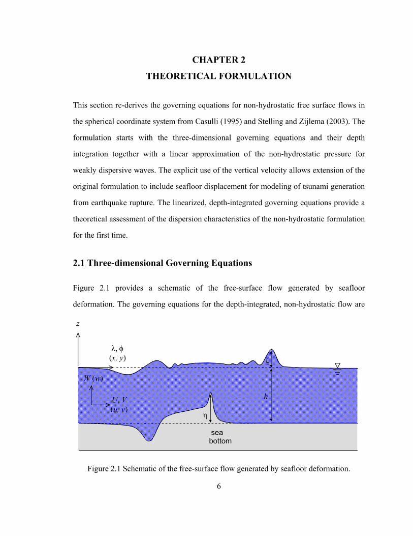
Figure 2.1 provides a schematic of the free-surface flow generated by seafloor
deformation. The governing equations for the depth-integrated, non-hydrostatic flow are
6
η
h
ζ
sea bottom
λ, φ (x, y)
U, V (u, v)
W (w)
z
Figure 2.1 Schematic of the free-surface flow generated by seafloor deformation.

derived in the spherical coordinate system from the three-dimensional Navier-Stokes
equations and the continuity equation. Gill (1982) and Kowalik and Murty (1993)
describe the governing equations for three-dimensional basin-wide ocean circulations in
the spherical coordinates (λ, φ, z) , in which λ is longitude, φ is latitude, and z denotes
distance normal to the earth surface, in the form:
( )φ−φ⎟⎟⎠
⎞⎜⎜⎝
⎛φ
+Ω−∂∂
+φ∂∂
+λ∂∂
φ+
∂∂ cossin
cos2
coswv
Ru
zuwu
Rvu
Ru
tu
λ+λ∂∂
φρ−= Ap
R cos1 (2.1)
φ⎟⎟⎠
⎞⎜⎜⎝
⎛φ
+Ω++∂∂
+φ∂∂
+λ∂∂
φ+
∂∂ sin
cos2
cosu
Ru
Rwv
zvwv
Rvv
Ru
tv
φ+φ∂∂
ρ−= Ap
R1 (2.2)
φ⎟⎟⎠
⎞⎜⎜⎝
⎛φ
+Ω−−∂∂
+φ∂
∂+
λ∂∂
φ+
∂∂ cos
cos2
cos
2
uR
uRv
zwww
Rvw
Ru
tw gA
zp
z −+∂∂
ρ−=
1 (2.3)
( ) 0coscos1
cos1
=∂∂
+φ∂φ∂
φ+
λ∂∂
φ zwv
Ru
R (2.4)
where R is the earth’s radius; (u, v, w) is flow velocity; t is time; Ω is the earth’s angular
velocity; ρ is water density; p is pressure; g is gravitational acceleration; and (Aλ, Aφ, Az)
is the viscous force.. The three-dimensional governing equations fully describe important
physics associated with tsunami modeling, but can be computationally intensive for
practical applications.
Following Casulli (1995), the pressure is decomposed into hydrostatic and non-
hydrostatic components as
( ) qzgp ρ+−ζρ= (2.5)
where q denotes the non-hydrostatic pressure. The z derivative of the hydrostatic pressure
term in (2.3) becomes
7

( )[ ] ( ) ggz
zg=−
ρρ
−=∂−ζρ∂
ρ− 101 (2.6)
With the pressure decomposition, the Navier-Stokes equations (2.1)-(2.3) reduce to the
three-dimensional non-hydrostatic momentum equations as
( )φ−φ⎟⎟⎠
⎞⎜⎜⎝
⎛φ
+Ω−∂∂
+φ∂∂
+λ∂∂
φ+
∂∂ cossin
cos2
coswv
Ru
zuwu
Rvu
Ru
tu
λ+⎟⎠⎞
⎜⎝⎛
λ∂∂
+λ∂ζ∂
φ−= Aq
R cos1 (2.7)
φ⎟⎟⎠
⎞⎜⎜⎝
⎛φ
+Ω++∂∂
+φ∂∂
+λ∂∂
φ+
∂∂ sin
cos2
cosu
Ru
Rwv
zvwv
Rvv
Ru
tv
φ+⎟⎟⎠
⎞⎜⎜⎝
⎛φ∂∂
+φ∂ζ∂
−= AqR1 (2.8)
φ⎟⎟⎠
⎞⎜⎜⎝
⎛φ
+Ω−−∂∂
+φ∂
∂+
λ∂∂
φ+
∂∂ cos
cos2
cos
2
uR
uRv
zwww
Rvw
Ru
tw
zAzq+
∂∂
−= (2.9)
Note the pressure in the vertical momentum equation (2.9) is driven primarily by the non-
hydrostatic components through the vertical velocity. The three-dimensional non-
hydrostatic formulation based on (2.7)-(2.9) and (2.4) has been extensively applied to
modeling of free surface flows involving ocean and coastal circulations (e.g., Mahadevan
et al., 1996a; Casulli and Stelling, 1998; Stansby and Zhou, 1998; and Stelling and
Busnelli, 2001). These models first compute the more stable hydrostatic solution and then
correct the solution with the non-hydrostatic pressure, which is implicitly solved from a
Poisson equation derived from the continuity equation. Mahadevan et al. (1996b) shows
that the pressure decomposition (2.5) in the non-hydrostatic formulation provides a more
stable solution and significantly improves computational efficiency in comparison to a
direct solution of (2.1)-(2.4).
8
9
Even though the pressure decomposition (2.5) improves computational efficiency, the
three-dimensional non-hydrostatic models are still computationally expensive. These
models require a large number of vertical grid cells or layers, restricting the application to
a small area or the computation with coarse resolution. It is practically impossible to
model tsunamis from generation, propagation, to runup with appropriate resolution using
a three-dimensional, non-hydrostatic model.
2.2 Depth-integrated Governing Equations
The earlier three-dimensional models define the non-hydrostatic pressure at the cell-
center, which requires a large number of vertical grid cells to describe its variation.
Stelling and Zijlema (2003) proposed a non-hydrostatic model with multi-layer and
depth-integrated formulations, which take advantage of the Keller box scheme (1971) for
vertical gradient approximation. The Keller box scheme (1971) defines the non-
hydrostatic pressure at cell interfaces to estimate the vertical gradient, and with a few
vertical layers, provides equivalent solutions to those of the three-dimensional non-
hydrostatic and Navier-Stokes models. The non-hydrostatic model can be developed in a
depth-integrated formulation by applying the Keller box scheme as in the multi-layer
formulation. A depth-integrated non-hydrostatic model is much more efficient and
enables modeling of the tsunami evolution processes with desired grid resolution over an
extended region.
The depth-integrated formulation is derived from the three dimensional, non-hydrostatic
governing equations (2.7)-(2.9) and (2.4). The boundary conditions at the free surface and
seafloor facilitate the formulation of the depth-integrated governing equations through the
Keller box scheme (1971). The flow depth is the distance between the two boundaries
defined as

D = ζ + (h – η) (2.10)
where ζ is the surface elevation measured from the still-water level, h is the water depth
defined at the still water level, and η is the seafloor displacement. Material derivatives of
the surface elevation and water depth give rise to the kinematic free surface and seafloor
boundary conditions as
φ∂ζ∂
+λ∂ζ∂
φ+
∂ζ∂
=Rv
Ru
tw
cos at z = ζ (2.11)
( ) ( )φ∂η−∂
−λ∂η−∂
φ−
∂η∂
=h
Rvh
Ru
tw
cos at z = – h+η (2.12)
Both the hydrostatic and non-hydrostatic pressure terms vanish at z = ζ to provide the
dynamic free surface boundary condition.
Tsunamis are long waves with weak dispersion characteristics. The vertical velocity w
generally follows a linear distribution between the seafloor and the free surface. The
Coriolis effects, the viscous dissipation, and the variation of the horizontal velocity in the
vertical direction are negligible in tsunami propagation. The kinematic boundary
conditions (2.11) and (2.12) are simplified to
φ∂ζ∂
+λ∂ζ∂
φ+
∂ζ∂
=RV
RU
tw
cos at z = ζ (2.13)
( ) ( )φ∂η−∂
−λ∂η−∂
φ−
∂η∂
=h
RVh
RU
tw
cos at z = – h+η (2.14)
where U and V are depth-averaged velocity components in the λ and φ directions, and the
vertical momentum equation (2.9) reduces to
tw∂∂
zq∂∂
−= (2.15)
10

Depth integration of (2.7), (2.8), (2.15), and (2.4) taking into account of the kinematic
boundary conditions (2.13) and (2.14) provides
λ∂ζ∂
φ−=φ⎟⎟
⎠
⎞⎜⎜⎝
⎛φ
+Ω−φ∂
∂+
λ∂∂
φ+
∂∂
cossin
cos2
cos RgV
RUU
RVU
RU
tU
DVUUfzdq
DR h
22
cos1 +
−λ∂∂
φ− ∫
ζ
η+−
(2.16)
φ∂ζ∂
−=φ⎟⎟⎠
⎞⎜⎜⎝
⎛φ
+Ω+φ∂
∂+
λ∂∂
φ+
∂∂
RgU
RUV
RVV
RU
tV sin
cos2
cos
DVUVfzdq
DR h
221 +−
φ∂∂
− ∫ζ
η+−
(2.17)
=∂∂
tW zd
zq
D h∫ζ
η+− ∂∂
−1 (2.18)
( ) ( ) ( ) 0coscos1
cos1
=φ∂φ∂
φ+
λ∂∂
φ+
∂η−ζ∂ DV
RUD
Rt (2.19)
where W is the depth-averaged velocity component in the z direction; f is a dimensionless
friction factor given in terms of Manning’s relative roughness coefficient n as
312
Dgnf = (2.20)
Standard hydraulic texts such as Chow (1959) and Chaudhry (1993) provide the Manning
coefficient as a function of materials and surface conditions, while Bretschneider et al.
(1986) determined typical values of the coefficient for tropical island terrain and
vegetation through measurements of wind profiles.
The momentum equations (2.16)-(2.18) contain integrals of the non-hydrostatic pressure
and the way they are evaluated will influence the dispersion characteristics of the
11

resulting governing equations. The non-hydrostatic pressure term in (2.16) can be derived
through the Leibniz rule of integration:
( )λ∂
η+−∂−
λ∂ζ∂
+λ∂∂
=λ∂∂
η+−ζ
ζ
η+−
ζ
η+−∫∫
hqqzdqzqd hhh
(2.21)
where qζ and q–h+b, are non-hydrostatic pressure at the free surface and seafloor,
respectively. The integration of non-hydrostatic pressure on the left hand side of (2.21) is
approximated as
⎥⎦
⎤⎢⎣
⎡⎟⎟⎠
⎞⎜⎜⎝
⎛ +λ∂∂
≈λ∂∂ η+−ζ
ζ
η+−∫ 2
h
h
qqDzqd (2.22)
Using (2.21) and (2.22), the non-hydrostatic pressure term in (2.16) can be rewritten in
the form:
( )λ∂
η+−ζ∂+
λ∂∂
=λ∂∂
η+−η+−
ζ
η+−∫
hqq
zdqh
h
h 21
21 (2.23)
The same procedure gives the non-hydrostatic pressure term in the φ-momentum equation
(2.17) as
( )φ∂
η+−ζ∂+
φ∂
∂=
φ∂∂
η+−η+−
ζ
η+−∫
hqq
zdqh
h
h 21
21 (2.24)
Note that qζ = 0 since the total pressure vanishes at the free surface. The vertical
momentum equation (2.18) can be simplified as
tW∂∂
Dq h η+−= (2.25)
The non-hydrostatic pressure in (2.23), (2.24), and (2.25) are now expressed in terms of
q–h+b defined on the seafloor.
Substitution of the non-hydrostatic pressure terms (2.23) and (2.24) into the horizontal
momentum equations (2.16) and (2.17) and the simplification of the z momentum
12

equation from (2.25), along with the continuity equation (2.19), give rise to the depth-
integrated, non-hydrostatic governing equations:
λ∂ζ∂
φ−=φ⎟⎟
⎠
⎞⎜⎜⎝
⎛φ
+Ω−φ∂
∂+
λ∂∂
φ+
∂∂
cossin
cos2
cos RgV
RUU
RVU
RU
tU
( )D
VUUfhDR
qqR
22
cos21
cos1
21 +
−λ∂
η+−ζ∂φ
−λ∂∂
φ− (2.26)
φ∂ζ∂
−=φ⎟⎟⎠
⎞⎜⎜⎝
⎛φ
+Ω+φ∂
∂+
λ∂∂
φ+
∂∂
RgU
RUV
RVV
RU
tV sin
cos2
cos
( )D
VUVfhDRqq
R
22
211
21 +
−φ∂
η+−ζ∂−
φ∂∂
− (2.27)
Dq
tW
=∂∂ (2.28)
( ) ( ) ( ) 0coscos1
cos1
=φ∂φ∂
φ+
λ∂∂
φ+
∂η−ζ∂ DV
RUD
Rt (2.29)
where q is now defined as the non-hydrostatic pressure at the seafloor. Because of the
assumption of a linear distribution for w, the vertical velocity is simply
2η+−ζ += hww
W (2.30)
which is the average value of w at the free surface and the seafloor given respectively in
(2.13) and (2.14). Except for the addition of the vertical momentum equation and the
non-hydrostatic pressure terms in the horizontal momentum equations, the governing
equations have the same structure as the nonlinear shallow-water equations. This
formulation allows a straightforward extension of existing nonlinear shallow-water
models for non-hydrostatic flows.
13

The governing equations in the spherical coordinate system (λ, φ) can be transformed into
the Cartesian system (x, y) for a relatively small region, where effects of the earth’s
curvature is insignificant. The distance in the x and y directions becomes
φλ= cosRx , (2.31) φ= Ry
The Coriolis terms in the horizontal momentum equations (2.26) and (2.27) vanish
0sincos
2 =φ⎟⎟⎠
⎞⎜⎜⎝
⎛φ
+Ω VR
U , 0sincos
2 =φ⎟⎟⎠
⎞⎜⎜⎝
⎛φ
+Ω UR
U (2.32)
Since the scale does not taper off in the north-south direction, we can simply set φ = 0.
These modifications provide the governing equations in the Cartesian coordinate system
in the form:
yUV
xUU
tU
∂∂
+∂∂
+∂∂
xg∂ζ∂
−=xq∂∂
−21 ( )
xh
Dq
∂η+−ζ∂
−21
DVUUf
22 +− (2.33)
yVV
xVU
tV
∂∂
+∂∂
+∂∂
yg∂ζ∂
−= yq∂∂
−21 ( )
yh
Dq
∂η+−ζ∂
−21
DVUVf
22 +− (2.34)
tW∂∂
Dq
= (2.35)
( ) ( ) ( ) 0=∂
∂+
∂∂
+∂
η−ζ∂y
VDx
UDt
(2.36)
where U and V are now the depth-averaged velocity components in the x and y directions.
The non-hydrostatic pressure is expressed in terms of the vertical acceleration through the
momentum equation (2.35). The kinematic boundary conditions (2.13) and (2.14)
describe the average vertical velocity in (2.35) as functions of U, V, ζ, and η to close the
depth-integrated governing equations for non-hydrostatic flows.
The advantage of the depth-integrated non-hydrostatic formulation is the form of the
dispersive terms, which are only the first derivative of the non-hydrostatic pressure. This
14

can be achieved because the non-hydrostatic pressure directly relates to the vertical
acceleration. On the other hand, the dispersive terms in Boussinesq-type equations are
expressed in term of the horizontal velocity, which requires additional temporal and
spatial differentiation to relate to the non-hydrostatic pressure.
2.3 Linear Dispersion Relation
The depth-integrated non-hydrostatic equations describe wave dispersion through the
non-hydrostatic pressure and vertical velocity. Although the basic assumptions are
consistent with those in the classical Boussinesq equations of Peregrine (1967), the
dispersion characteristics might differ due to the variables employed and truncation of
terms in the derivation of the governing equations. This section derives the linear
dispersion relation for the depth-integrated non-hydrostatic equations for direct
comparison with those from the classical Boussinesq equations and Airy wave theory.
Although the non-hydrostatic and the Boussinesq equations are nonlinear, the comparison
of their linear dispersion characteristics provides a baseline for assessment.
The first step is to derive a linearized version of the depth-integrated, non-hydrostatic
governing equations. After dropping the nonlinear terms and setting η = 0, the governing
equations in the x direction from (2.33) to (2.36) become
021
21
=∂∂
−∂∂
+∂ζ∂
+∂∂
xh
hq
xq
xg
tU (2.37)
02
=−⎟⎟⎠
⎞⎜⎜⎝
⎛ +
∂∂ −ζ
hqww
th (2.38)
0=∂∂
+∂ζ∂
xUh
t (2.39)
15

The one-dimensional kinematic conditions on the free surface and the seafloor, with the
vertical variation of the horizontal velocity neglected and η = 0, become
xU
tw
∂ζ∂
+∂ζ∂
=ζ (2.40)
xhUw h ∂∂
−=− (2.41)
The non-hydrostatic pressure q in terms of ζ and U can be obtained from the vertical
momentum equation (2.38) by substitution of the kinematic boundary conditions (2.40)
and (2.41) as
2
2
21
thq∂ζ∂
=xt
hU∂∂ζ∂
+2
21 ( )
xh
tUh
∂−ζ∂
∂∂
+21 (2.42)
The x-derivative of q is expanded by the chain rule as
=∂∂
xq
2
2
21
txh∂ζ∂
∂∂
xth
∂∂ζ∂
+ 2
3
21
xtx
Uh∂∂ζ∂
∂∂
+2
21
xtU
xh
∂∂ζ∂
∂∂
+2
21
2
3
21
xthU
∂∂ζ∂
+
( )
xh
tU
xh
∂−ζ∂
∂∂
∂∂
+21 ( )
xh
xtUh
∂−ζ∂
∂∂∂
+21 ( )
2
2
21
xh
tUh
∂−ζ∂
∂∂
+ (2.43)
Substituting (2.42) and (2.43) into the horizontal momentum equation (2.37), we have the
horizontal momentum equation in terms of ζ and U as
tU∂∂
xg∂ζ∂
+xt
h∂∂ζ∂
+ 2
3
41
xtU
xhh
∂∂∂
∂∂
−2
41
tU
xhh∂∂
∂∂
− 2
2
41 0
41
2
2
=∂ζ∂
∂∂
−tx
h (2.44)
The non-hydrostatic pressure and vertical velocity are now expressed by a third-order
derivative of the surface elevation and three additional terms related to the depth gradient.
The exact linear dispersion relation from Airy wave theory is for constant water depth.
The Boussinesq-type equations were initially derived for constant water depth (Peregrine,
16

1967; and Madsen et al., 1991). To provide a direct comparison, the depth-gradient terms
in (2.44) are dropped. The resulting governing equations for constant water depth become
tU∂∂
xg∂ζ∂
+ 041
2
3
=∂∂ζ∂
+xt
h (2.45)
0=∂∂
+∂ζ∂
xUh
t (2.46)
Following Madsen et al. (1991) and Nwogu (1993), the linear dispersive relation is
derived by considering a system small amplitude periodic waves in the form:
( ctxkie −ζ=ζ 0)
)
(2.47)
( ctxkieUU −= 0 (2.48)
where k and c denote the wave number and celerity. Substituting (2.47) and (2.48) into
the linearized depth-integrated, non-hydrostatic equation (2.45) and (2.46) yields the
dispersion relation:
2
2
)(411 kh
ghc+
= (2.49)
The linear dispersion relation from the classical Boussinesq equations of Peregrine (1967)
is given by
2
2
)(311 kh
ghc+
= (2.50)
The exact linear dispersion relation of Airy wave theory is in the form:
khkhghc )tanh(2 = (2.51)
17

Figure 2.2 Linear dispersion relation. - - - -, exact solution; -⋅-⋅-⋅-, classical Boussinesq equation of Peregrine (1967); ⎯⎯ (red), depth-integrated, non-hydrostatic equations.
Figure 2.2 compares the linear dispersion relations (2.49) and (2.50) with the exact
relation (2.51). The applicable range of a model is up to an error of 5% in the linear
dispersion relation according to Madsen et al. (1991). Within the intermediate water
depth π/10 < kh < π, the dispersion relation of the depth-integrated non-hydrostatic
equations has an error less than 5%. The classical Boussinesq equation of Peregrine
(1967) has an error of 5% at kh = 1.35 and a maximum of 20% within the intermediate
depth range. This provides a theoretical proof of the observations by Stelling and Zijlema
(2003) and Walters (2005) that their non-hydrostatic models produce better dispersion
characteristics than the classical Boussinesq equations.
To gain understanding of the dispersion characteristics between the non-hydrostatic and
the Boussinesq equations, the momentum equation (2.45) is rewritten with the continuity
equation (2.46) to express the dispersive term as a function of the horizontal velocity.
After dropping the bottom-gradient term, we have
18

xg
tU
∂ζ∂
+∂∂
⎟⎟⎠
⎞⎜⎜⎝
⎛∂∂
∂∂∂
−tx
Ux
h2
2
41 0= (2.52)
This has the same form as the momentum equation of the linearized classical Boussinesq
equations as
xg
tU
∂ζ∂
+∂∂
⎟⎟⎠
⎞⎜⎜⎝
⎛∂∂
∂∂∂
−tx
Ux
h2
2
31 0= (2.53)
The only difference is in the coefficient of the linear dispersive term that mirrors the
respective linear dispersion relations (2.49) and (2.50). The major difference between the
two approaches is the use of the irrotational flow condition in the classical Boussinesq
equations to express the vertical velocity in terms of the horizontal velocity. This
introduces an additional depth-integration step in the derivation of the classical
Boussinesq equations. The depth-integrated, non-hydrostatic formulation, on the other
hands, utilizes an approximated vertical momentum equation to account for vertical
velocity effects, which are weakly coupled with the horizontal velocity through the
governing equations. When the vertical velocity variation over a water column deviates
from the long-wave assumptions, the additional integration in the classical Boussinesq
equations could amplify the error through the horizontal velocity, which is the primary
variable in the physical problem. This is reflected in the comparison of the dispersion
relations in Figure 2.2.
19

CHAPTER 3
NUMERICAL FORMULATION
The numerical formulation includes the solution schemes for the hydrostatic and non-
hydrostatic components of the governing equations in both the spherical and Cartesian
grid systems. The finite difference scheme utilizes the upwind flux approximation of
Mader (1988) in the continuity equation as well as the calculation of the advective terms
in the horizontal momentum equations. Figure 3.1 shows the space-staggered grid for the
computation. The model calculates the horizontal velocity components U and V at the cell
interface and the free surface elevation ζ, the non-hydrostatic pressure q, and the vertical
velocity W at the cell center, where the water depth h is defined.
20
λ (x)
φ (y)
j –1 j j +1
k –1
k +1
k Uj,k Vj,k
ζ j,k
Figure 3.1 Definition sketch of spatial grid.

3.1 Hydrostatic Solution in Spherical Grids
The hydrostatic model utilizes an explicit scheme for the solution. Integration of the
continuity equation (2.29) provides an update of the surface elevation at the center of cell
(j, k) in terms of the fluxes, FLX and FLY, along the longitude and latitude at the cell
interfaces as
( )k
kjkjmkj
mkj
mkj
mkj R
FLXFLXt
φλΔ
−Δ−η−η+ζ=ζ +++
cos,,1
,1
,,1
,
( ) ( )
k
kkjkkj
RFLYFLY
tφφΔ
φΔ+φ−φΔ+φΔ− −−
cos2cos2cos 11,, (3.1)
where m denotes the time step, Δt the time step size, and Δ λ and Δφ the respective grid
sizes. The upwind scheme gives the flux terms as
( ) ( )2
,,,1,11,,
1,1
1,
mkjkj
mkjkjm
kjm
kjmn
mkj
mpkj
hhUUUFLX
η−+η−+ζ+ζ= −−++
−+ (3.2a)
( ) ( )2
1,1,,,1,1,
1,
1,
mkjkj
mkjkjm
kjm
kjm
nm
kjmpkj
hhVVVFLY +++
+++ η−+η−
+ζ+ζ= (3.2b)
in which
2,,
mkj
mkjm
p
UUU
+= ,
2,,
mkj
mkjm
n
UUU
−= ;
2,,mkj
mkjm
p
VVV
+= ,
2,,mkj
mkjm
n
VVV
−= (3.3)
The upwind flux approximation (3.2) extrapolates the surface elevation from the upwind
cell, while the water depth takes on the average value from the two adjacent cells (Mader,
1988). This represents a departure from most existing shallow-water models that
extrapolate the flow depth instead (Kowalik and Murty, 1993; and Titov and Synolakis,
1998). In these models, the flux is determined with a second-order scheme
( ) ( )2
,,,,1,1,11,,
mkjkj
mkj
mkjkj
mkjm
kjkj
hhUFLX
η−+ζ+η−+ζ= −−−+ (3.4a)
21

( ) ( )2
1,1,1,,,,1,,
mkjkj
mkj
mkjkj
mkjm
kjkj
hhVFLY ++++ η−+ζ+η−+ζ
= (3.4b)
This approach uses average values of the surface elevations and water depths from
adjacent cells to determine the flux and is equivalent to the flux-based formulation of the
nonlinear shallow-water equations (e.g., Shuto and Goto, 1978; Liu et al., 1995b; and
Imamura, 1996).
The horizontal momentum equations provide the velocity components U and V at (m+1)
in (3.2) for the update of the surface elevation in (3.1). In the spatial discretization, the
average values of U and V are used in the horizontal momentum equations. These
average velocity components are defined by
( mkj
mkj
mkj
mkj
mkjy UUUUU 1,1,1,1,, 4
1++++ +++= ) (3.5)
( mkj
mkj
mkj
mkj
mkjx VVVVV 1,1,1,1,, 4
1−−−− +++= ) (3.6)
Integration of the λ and φ-momentum equations (2.26) and (2.27), with the non-
hydrostatic terms omitted, provides the hydrostatic solution for the horizontal velocity
( )mkj
mkj
k
mkj
mkj R
tgUU ,1,,1
, cos~
−+ ζ−ζ
φλΔΔ
−= km
kjxk
mkj V
RU
t φ⎟⎟⎠
⎞⎜⎜⎝
⎛
φ+ΩΔ+ sin
cos2 ,
,
( ) ( )mkj
mkj
mn
k
mkj
mkj
mp
k
UUUR
tUUUR
t,,1,1, coscos
−φλΔ
Δ−−
φλΔΔ
− +−
( ) ( )mkj
mkj
mnx
mkj
mkj
mpx UUV
RtUUV
Rt
,1,1,, −φΔ
Δ−−
φΔΔ
− +−
( ) ( )( )3
4
,,1
2
,2
,,2
mkj
mkj
mkjx
mkj
mkj
DD
VUtUgn
+
+Δ−
−
(3.7)
22

( )mkj
mkj
mkj
mkj R
tgVV ,1,,1
,~ ζ−ζ
φΔΔ
−= ++
( ) ( )2sin2cos
2,
, φΔ+φ⎟⎟
⎠
⎞
⎜⎜
⎝
⎛
φΔ+φ+ΩΔ− k
mkjy
k
mkjy
UR
Ut
( ) ( ) ( ) ( )mkj
mkj
mny
k
mkj
mkj
mpy
k
VVUR
tVVUR
t,,1,1, 2cos2cos
−φΔ+φλΔ
Δ−−
φΔ+φλΔΔ
− +−
( ) ( )mkj
mkj
mn
mkj
mkj
mp VVV
RtVVV
Rt
,1,1,, −φΔ
Δ−−
φΔΔ
− +−
( ) ( )( )3
4
1,,
2,
2
,,2
mkj
mkj
mkj
mkjy
mkj
DD
VUtVgn
++
+Δ− (3.8)
where the subscripts p and n indicates upwind and downwind approximations of the
advective speeds.
Most nonlinear shallow-water models, which use the advective speeds from (3.3) in the
momentum equations, cannot capture flow discontinuities associated with breaking
waves or hydraulic jumps. Stelling and Duinmeijer (2003) derived an alternative
discretization of the advective speeds that conserves energy or momentum across flow
discontinuities. Momentum conservation provides a better description of bores or
hydraulic jumps that mimic breaking waves in depth-integrated flows. This is also
consistent with the finite volume method with a Riemann solver (e.g., Wei et al., 2006;
Wu and Cheung, 2008; and George, 2010). We adapt the momentum-conserved
advection scheme from Stelling and Duinmeijer (2003) with the present upwind flux
approach to provide the advective speeds as
⎪⎪
⎩
⎪⎪
⎨
⎧
=
≠+
=
0if0
0if2
ˆˆ
,
,,,
mkj
mkj
m
kjpm
kjp
mp
U
UUU
U ,
⎪⎪
⎩
⎪⎪
⎨
⎧
=
≠−
=
0if0
0if2
ˆˆ
,
,
,,
mkj
mkj
mkjn
mkjn
mn
U
UUU
U (3.9a)
23

⎪⎪
⎩
⎪⎪
⎨
⎧
=
≠+
=
0if0
0if2
ˆˆ
,
,,,
mkj
mkj
m
kjpm
kjp
mp
V
VVV
V ,
⎪⎪
⎩
⎪⎪
⎨
⎧
=
≠−
=
0if0
0if2
ˆˆ
,
,
,,
mkj
mkj
mkjn
mkjn
mn
V
VVV
V (3.9b)
in which
mkj
mkj
mkjpm
kjp DDFLU
U,,1
,
,
2ˆ+
=−
, mkjnU ,
ˆm
kjm
kj
mkjn
DDFLU
,,1
,2+
=−
(3.10a)
mkj
mkj
mkjpm
kjp DDFLV
V1,,
,
,
2ˆ++
= , mkjnV ,
ˆm
kjm
kj
mkjn
DDFLV
1,,
,2
++= (3.10b)
where the flux for a positive flow ( ) is given by 0, >mkjU
( )
⎪⎪⎪⎪
⎩
⎪⎪⎪⎪
⎨
⎧
<<+
≥<ζ+η−+
>⎟⎟⎠
⎞⎜⎜⎝
⎛ ζ+ζ+η−
+
=
−−−
−−−−−−
−−−
−−−
mkj
mkj
mkj
mkj
mkjm
kj
mkj
mkj
mkj
mkj
mkjkj
mkj
mkj
mkj
mkj
mkjm
kjkj
mkj
mkj
mkjp
UUUDD
U
UUUhUU
UhUU
FLU
,1,,1,,1
,
,1,,1,1,1,1,,1
,1,1,2
,1,1,,1
,
and0if2
and0if2
0 if22
(3.11a)
and the flux for a negative flow ( ) is 0, <mkjU
( )
⎪⎪⎪⎪
⎩
⎪⎪⎪⎪
⎨
⎧
<>+
≥>ζ+η−+
<⎟⎟⎠
⎞⎜⎜⎝
⎛ ζ+ζ+η−
+
=
++−
+++
+++
mkj
mkj
mkj
mkj
mkjm
kj
mkj
mkj
mkj
mkj
mkjkj
mkj
mkj
mkj
mkj
mkjm
kjkj
mkj
mkj
mkjn
UUUDD
U
UUUhUU
UhUU
FLU
,1,,1,,1
,
,1,,1,,,,1,
,1,1,
,,,1,
,
and0if2
and0if2
0 if22
(3.11b)
Similarly, the flux for is given by 0, >mkjV
24

( )
⎪⎪⎪⎪
⎩
⎪⎪⎪⎪
⎨
⎧
<<+
≥<ζ+η−+
>⎟⎟⎠
⎞⎜⎜⎝
⎛ ζ+ζ+η−
+
=
−−+
−−−
−−−
mkj
mkj
mkj
mkj
mkjm
kj
mkj
mkj
mkj
mkj
mkjkj
mkj
mkj
mkj
mkj
mkjm
kjkj
mkj
mkj
mkjp
VVVDD
V
VVVhVV
VhVV
FLV
1,,1,1,,
,
1,,1,,,,,1,
1,,1,
,,,1,
,
and0if2
and0if2
0if22
(3.11c)
and the flux for is 0, <mkjV
( )
⎪⎪⎪⎪
⎩
⎪⎪⎪⎪
⎨
⎧
<>+
≥>ζ+η−+
<⎟⎟⎠
⎞⎜⎜⎝
⎛ ζ+ζ+η−
+
=
+++
++++++
+++
+++
mkj
mkj
mkj
mkj
mkjm
kj
mkj
mkj
mkj
mkj
mkjkj
mkj
mkj
mkj
mkj
mkjm
kjkj
mkj
mkj
mkjn
VVVDD
V
VVVhVV
VhVV
FLV
1,,1,1,,
,
1,,1,1,1,1,1,,
1,2,1,
1,1,1,,
,
and0if2
and0if2
0 if22
(3.11d)
The advective speeds pyU , nyU , pxV , and nxV in (3.7) and (3.8) can be obtained from
(3.9) to (3.11) with average values of Uj,k and Vj,k in the form of (3.5) and (3.6) as well as
the average values of ζj,k and hj,k calculated in the same way. This completes the
numerical formulation for the nonlinear shallow-water equations in describing
hydrostatic flows.
In comparison, Stelling and Duinmeijer (2003) derived the momentum-conserved
advection approximation from the conservative form of the nonlinear shallow-water
equations. The resulting momentum equations are the same as the non-conservative form
with the exception of the advective speeds, which are given by
mkj
mkj
mkjm
kjp DDFLUU
,,1
,1
,
2ˆ+
=−
− , mkjnU ,
ˆm
kjm
kj
mkj
DDFLU
,,1
,2+
=−
(3.12)
The flux at the cell center is obtained from
25

2,1,
,
mkj
mkjm
kjFLUFLU
FLU ++= (3.13)
where
( ) ( )[ ] 0for0for0for
,max,min ,
,
,
,,1,,1,
,,
,1,
,
=<>
⎪⎩
⎪⎨
⎧
+ζζ=
−−
−
mkj
mkj
mkj
kjkjm
kjm
kjm
kj
mkj
mkj
mkj
mkj
mkj
UUU
hhUDUDU
FLU (3.14)
Note that the averaged fluxes m
kjFLU ,1− and m
kjFLU , in (3.12) are equivalent to
and in (3.11a) and (3.11b) of the present scheme. Their upwind scheme (3.14)
extrapolates the flow depth and calculates the average flux
mkjpFLU ,
mkjnFLU ,
mkjFLU , at the cell center from
the interface values through (3.13). In contrast, the present approach extrapolates the
surface elevation at the cell interface and directly calculates the fluxes and
at the cell center from (3.11a) and (3.11b). With the water depth defined at the
cell center, any discontinuity is due entirely to the surface elevation. The present upwind
scheme avoids errors from depth extrapolation and most importantly improves the
capability to capture flow discontinuities. This becomes essential when the topography is
irregular and wave breaking is energetic.
mkjp ,FLU
mkjn ,FLU
3.2 Non-hydrostatic Solution in Spherical Grids
This section describes the development of the non-hydrostatic solution from the nonlinear
shallow-water results as well as the bottom pressure and vertical velocity terms neglected
in the hydrostatic formulation. Integration of the non-hydrostatic terms in the horizontal
momentum equations completes the update of the horizontal velocity from (3.7) and (3.8)
( ) ( )2cos2cos
~ 1,1
1,
1,1
1,
,1
,1
,
+−
++−
+++ −
φλΔΔ
−+
φλΔΔ
−=m
kjm
kj
k
mkj
mkj
kjk
mkj
mkj
qqR
tqqA
RtUU (3.15)
( ) ( )22
~ 1,
11,
1,
11,
,1
,1
,
+++
+++++ −
φΔΔ
−+
φΔΔ
−=m
kjm
kjm
kjm
kjkj
mkj
mkj
qqR
tqqB
RtVV (3.16)
26

where
( ) ( )( )m
kjm
kj
mkjkj
mkj
mkjkj
mkj
kj DDhh
A,1,
,1,1,1,,,,
−
−−−
+
η+−ζ−η+−ζ= (3.17a)
( ) ( )( )m
kjm
kj
mkjkj
mkj
mkjkj
mkj
kj DDhh
B1,,
,,,1,1,1,,
+
+++
+
η+−ζ−η+−ζ= (3.17b)
Discretization of the vertical momentum equation (2.28) gives the vertical velocity at the
free surface as
( ) 1,
,,
1,,
1,
2 +++ Δ+−−= m
kjmkj
mkjb
mkjb
mkjs
mkjs q
Dtwwww (3.18)
The vertical velocity at the seafloor is evaluated from the boundary condition (2.14) as
tw
mkj
mkjm
kjb Δ
η−η=
++ ,
1,1
,
( ) ( ) ( ) ( )k
mkjkj
mkjkjm
nzk
mkjkj
mkjkjm
pz Rhh
UR
hhU
φλΔ
η−−η−−
φλΔ
η−−η−− ++−−
coscos,,,1,1,1,1,,
( ) ( ) ( ) ( )φΔ
η−−η−−
φΔ
η−−η−− ++−−
Rhh
VR
hhV
mkjkj
mkjkjm
nz
mkjkj
mkjkjm
pz,,1,1,1,1,,, (3.19)
in which
2,,
mkjz
mkjzm
pz
UUU
+= ,
2,,
mkjz
mkjzm
nz
UUU
−= ;
2,,
mkjz
mkjzm
pz
VVV
+= ,
2,,
mkjz
mkjzm
nz
VVV
−= (3.20)
where
2,1,
,
mkj
mkjm
kjz
UUU ++
= , 2
1,,,
mkj
mkjm
kjz
VVV −+
= (3.21)
The horizontal velocity components and the vertical velocity at the free surface are now
expressed in terms of the non-hydrostatic pressure.
27

Analogous to the solution of the three-dimensional governing equations, the non-
hydrostatic pressure is calculated implicitly using the continuity equation (2.4)
discretized in the form
1,+mkjq
( ) ( )0
cos2cos2cos
cos ,
1,
1,1
11,
1,
1,
1,1 =
−+
φφΔ
φΔ+φ−φΔ+φ+
φλΔ
− ++−
+−
++++
mkj
mkjb
mkjs
k
kmkjk
mkj
k
mkj
mkj
D
wwR
VVR
UU
(3.22)
Substitution of (3.15), (3.16) and (3.18) into the continuity equation (3.22) gives a linear
system of Poisson-type equations at each cell
kjm
kjkjm
kjkjm
kjkjm
kjkjm
kjkj QCqPCqPTqPBqPRqPL ,1
,,1
1,,1
1,,1,1,
1,1, =++++ ++
++−
++
+− (3.23)
where the coefficients are
( )( )kj
kkj A
RtPL ,22, 1
2cos1
+−λΔ
Δφ
=
( )( )kj
kkj A
RtPR ,122, 1
2cos1
+−−λΔ
Δφ
=
( )( )
( )1,21
, 12cos
2cos−
− +−φΔ
Δφ
φΔ+φ= kj
k
kkj B
RtPB
( )( )
( )kjk
kkj B
RtPT ,2, 1
2cos2cos
−−φΔ
ΔφφΔ+φ
=
( )( ) ( )[ ]kjkj
kkj AA
RtPC ,1,22, 11
2cos1
+−++λΔ
Δφ
=
( )
( ) ( ) ( ) ( )[ ]2cos12cos12cos
11,1,2 φΔ+φ−+φΔ+φ+
φΔΔ
φ+ −− kkjkkj
k
BBR
t
2, )(
2m
kjDtΔ
+ (3.24)
and the forcing term is
28

( ) ( )k
kmkjk
mkj
k
mkj
mkj
kj RVV
RUU
QφφΔ
φΔ+φ−φΔ+φ−
φλΔ
−−= −
+−
++++
cos2cos~2cos~
cos
~~1
11,
1,
1,
1,1
,
mkj
mkjb
mkjb
mkjs
Dwww
,
1,,, 2 +−+
− (3.25)
Assembly of (3.23) at all grid cells gives rise to a matrix equation in the form of
[ ] QqP = (3.26)
which provides the non-hydrostatic pressure at each time step. The Poisson-type equation
(3.23) defines the physics of the non-hydrostatic processes through the non-dimensional
parameters, Ajk, and Bjk, and the forcing term Qj,k, which describe the seafloor, free-
surface, and velocity gradients in the generation and modification of dispersive waves.
The vertical component of the flow, important for sustaining dispersive processes, is
imparted through the bottom and surface slopes in terms of the horizontal flow
components from the boundary conditions (2.13) and (2.14). As the ocean bottom and
surface gradients start to change abruptly at shelf breaks and around steep seamounts and
canyons, the coefficients Ajk and Bjk may strongly influence the solution process. The
equation type may even change in the runup calculation as the water depth hj,k varies
from positive to negative across the waterline and the values of Ajk and Bjk can be greater
than unity. The matrix equation (3.26), in which the matrix [P] is non-symmetric, can be
solved by the strongly implicit procedure (SIP) of Stone (1968).
At each time step, the computation starts with the calculation of the hydrostatic solution
of the horizontal velocities using (3.7) and (3.8). The non-hydrostatic pressure is then
calculated using (3.26) and the horizontal velocities are updated with (3.15) and (3.16) to
account for the non-hydrostatic effects. The computation for the non-hydrostatic solution
is complete with the calculation of the surface elevation as well as the free surface and
the bottom vertical velocities from (3.1), (3.18) and (3.19), respectively.
29

3.3. Solutions in Cartesian Grids
The numerical formulation in the Cartesian coordinate system can be obtained from the
discretized form of the coordinate transformation in (2.31) and (2.32). The grid spacing in
the x and y directions becomes
kRx φλΔ=Δ cos , φΔ=Δ Ry (3.27)
The Coriolis terms in horizontal momentum equations (3.7) and (3.8) vanish for
modeling of a small coastal region or a laboratory experiment
0sincos
2 ,, =φ⎟
⎟⎠
⎞⎜⎜⎝
⎛
φ+Ω k
mkjx
k
mkj V
RU
(3.28a)
( ) ( ) 02sin2cos
2,
, =φΔ+φ⎟⎟
⎠
⎞
⎜⎜
⎝
⎛
φΔ+φ+Ω k
mkjy
k
mkjy
UR
U (3.28b)
The explicit time integration of the depth-integrated continuity equation becomes
( ) ( )yFLYFLY
tx
FLXFLXt kjkjkjkjm
kjm
kj Δ
−Δ−
Δ
−Δ−ζ=ζ −++ 1,,,,1
,1
, (3.29)
where the flux terms are estimated from (3.2). The integration of the hydrostatic terms in
the momentum equations gives
( ) ( ) ( mkj
mkj
mn
mkj
mkj
mp
mkj
mkj
mkj
mkj UUU
xtUUU
xt
xtgUU ,,1,1,,1,,
1,
~−
Δ)Δ
−−ΔΔ
−ζ−ζΔΔ
−= +−−+
( ) ( )mkj
mkj
mnx
mkj
mkj
mpx UUV
ytUUV
yt
,1,1,, −ΔΔ
−−ΔΔ
− +−
( ) ( )
( )34
,,1
2
,2
,,2
mkj
mkj
mkjx
mkj
mkj
DD
VUtUgn
+
+Δ−
−
(3.30)
30

( ) ( ) ( )mkj
mkj
mny
mkj
mkj
mpy
mkj
mkj
mkj
mkj VVU
xtVVU
xt
ytgVV ,,1,1,,1,,
1,
~ −ΔΔ
−−ΔΔ
−ζ−ζΔΔ
−= +−++
( ) ( )mkj
mkj
mn
mkj
mkj
mp VVV
ytVVV
yt
,1,1,, −ΔΔ
−−ΔΔ
− +−
( ) ( )
( )34
1,,
2,
2
,,2
mkj
mkj
mkj
mkjy
mkj
DD
VUtVgn
++
+Δ− (3.31)
The momentum-conserved advection scheme (3.9)-(3.11) provides the advective speeds
to handle flow discontinuities.
The time integration of the non-hydrostatic terms in the horizontal momentum equations
becomes
( ) ( )22
~ 1,1
1,
1,1
1,
,1
,1
,
+−
++−
+++ −
ΔΔ
−+
ΔΔ
−=m
kjm
kjm
kjm
kjkj
mkj
mkj
qqxtqq
AxtUU (3.32)
( ) ( )22
~ 1,
11,
1,
11,
,1
,1
,
+++
+++++ −
ΔΔ
−+
ΔΔ
−=m
kjm
kjm
kjm
kjkj
mkj
mkj
qqytqq
BytVV (3.33)
where
( ) (( )
)m
kjm
kj
kjm
kjkjm
kjkj DD
hhA
,1,
,1,1,,,
−
−−
+
−ζ−−ζ= ,
( ) ( )( )m
kjm
kj
kjm
kjkjm
kjkj DD
hhB
1,,
,,1,1,,
+
++
+
−ζ−−ζ= (3.34)
The free surface and seafloor vertical velocities are given by
( ) 1,
,,
1,,
1,
2 +++ Δ+−−= m
kjmkj
mkjb
mkjb
mkjs
mkjs q
Dtwwww (3.35)
xhh
Uxhh
Uw kjkjmnz
kjkjmpz
mkjb Δ
−−
Δ
−−= +−+ ,,1,1,1
, yhh
Vyhh
V kjkjmnz
kjkjmpz Δ
−−
Δ
−− +− ,1,1,, (3.36)
where the advective speeds are given by (3.20) and (3.21). The horizontal velocity and
the free surface vertical velocity, which are expressed in terms of the non-hydrostatic
31

pressure in (3.32) (3.33) and (3.35), update the hydrostatic solution to account for wave
dispersion effects.
The non-hydrostatic pressure is calculated implicitly using the three-dimensional
continuity equation (2.4) along with the coordinate transformation (2.31) and discretized
in the form:
1,+mkjq
0,
1,
1,
11,
1,
1,
1,1 =
−+
Δ−
+Δ− +++
−+++
+m
kj
mkjb
mkjs
mkj
mkj
mkj
mkj
Dww
yVV
xUU
(3.37)
The linear system of Poisson-type equations (3.23) is obtained by substitution of (3.32),
(3.33) and (3.35) into the continuity equation (3.37). The resulting coefficients and the
forcing term in the Cartesian grid are
( kjkj A )xtPL ,2, 1
2+−
ΔΔ
=
( )kjkj AxtPR ,12, 1
2 +−−ΔΔ
=
( )1,2, 12 −+−ΔΔ
= kjkj BytPB
( )kjkj BytPT ,2, 1
2−−
ΔΔ
=
( ) ( )[ ] ( ) ( )[ ] 2,
,1,2,1,2, )(211
211
2 mkj
kjkjkjkjkj DtBB
ytAA
xtPC Δ
+−++ΔΔ
+−++ΔΔ
= −+ (3.38)
yVV
xUU
Qmkj
mkj
mkj
mkj
kj Δ
−−
Δ
−−=
+−
++++
11,
1,
1,
1,1
,
~~~~
mkj
mkjb
mkjb
mkjs
D
www
,
1,,, 2 +−+
− (3.39)
The solution procedure is identical to that followed for the spherical coordinate system.
The computation starts with the hydrostatic solution of the horizontal velocities using
(3.30) and (3.31). The matrix equation (3.26) with the coefficients and forcing term from
(3.38) and (3.39) provides non-hydrostatic pressure and (3.32) and (3.33) updates the
32

33
horizontal velocity to account for the non-hydrostatic effects. The non-hydrostatic
solution is complete with the calculation of the surface elevation and the vertical
velocities from (3.29), (3.35), and (3.36).

34
CHAPTER 4
IMPLEMENTATION FOR TSUNAMI MODELING
The depth-integrated, non-hydrostatic model provides a general framework to describe
dispersion and breaking of ocean waves over variable bottom. This section discusses its
implementation with a wet-dry moving boundary condition, a two-way grid-nesting
scheme, and a bathymetry-smoothing strategy for modeling of the tsunami evolution
processes from generation to runup. The wet-dry moving boundary condition tracks the
interface between water and dry land to model the runup and drawdown processes at the
coast. The proposed two-way, grid-nesting scheme utilizes a flexible indexing system
that enables adaptation of inter-grid boundaries to topographic features for optimal
resolution and computational efficiency. The smoothing scheme generalizes the stability
requirements of Horrillo et al. (2006) to remove small-scale bathymetric features in
relation to the water depth that cannot be resolved by non-hydrostatic or Boussinesq-type
models.
4.1 Wet-Dry Moving Boundary Condition
For inundation or runup calculations, special numerical treatments are necessary to
describe the moving waterline in the swash zone. The present non-hydrostatic model
tracks the interface between wet and dry cells using the approach of Kowalik and Murty
(1993), which was originally developed for hydrostatic flow. The basic idea is to
extrapolate the numerical solution from the wet region onto the beach. The non-
hydrostatic pressure is set to be zero at the wet cells along the wet-dry interface to
conform to the physical problem and to improve stability of the scheme.

The moving waterline scheme provides an update of the wet-dry interface as well as the
associated flow depth and velocity at the beginning of every time step. A marker
first updates the wet-dry status of each cell based on the flow depth and surface
elevation. If the flow depth
mkjCELL ,
,mj kD is positive, the cell is under water and , and
if
1, =mkjCELL
,mj kD
CELL
is zero or negative, the cell is dry and . This captures the retreat of the
waterline in an ebb flow. The surface elevation along the interface then determines any
advancement of the waterline. For flows in the positive λ or x direction, if is dry
and is wet, is reevaluated as
0, =mkjCELL
mkjCELL ,
mkj ,1−
mkj ,CELL
mkjCELL , = 1 (wet) if kj
mkj h ,,1 −>ζ −
mkjCELL , = 0 (dry) if kj
mkj h ,,1 −≤ζ −
If becomes wet, the scheme assigns the flow depth and velocity at the cell as mkjCELL ,
kjm
kjm
kj hD ,,1, +ζ= − , , 1m m
,j k jU U −= k
The marker is then updated for flows in the negative direction. The same
procedures are implemented in the φ or y direction to complete the wet-dry status of the
cell. If water flows into a new wet cell from multiple directions, the flow depth is
averaged.
mkjCELL ,
Once the wet-dry cell interface is open by setting , the flow depth 1, =mkjCELL ,
mj kD and
velocity ( ,mj kU , ) are assigned to the new wet cell to complete the update of the wet-
dry interface at time step m. The surface elevation and the flow velocity (
mkjV ,
1,+ζmkj
1,
mj kU + ,
) over the computational domain are obtained from integration of the momentum
and continuity equations along with the implicit solution of the non-hydrostatic pressure
as outlined in Sections 3.1 and 3.2. The moving waterline scheme is then repeated to
update the wet-dry interface at the beginning of the (m+1) time step. This approach
1,+m
kjV
35

36
remains stable and robust for the non-hydrostatic flows without artificial dissipation
mechanisms.
4.2 Grid-nesting Scheme
Most grid-nesting schemes for hydrostatic models use a system of rectangular grids with
the fluxes as input variables to a fine inner grid and the surface elevation as output to the
outer grid (e.g., Liu et al., 1995b; Goto et al., 1997; Wei et al., 2003; Yamazaki et al.,
2006; and Sánchez and Cheung, 2007). A non-hydrostatic model needs to input the
velocity, surface elevation as well as the non-hydrostatic pressure to ensure propagation
of breaking and dispersion waves across inter-grid boundaries. Linear interpolation of
these quantities from the outer grid along the inter-grid boundary provides the input to the
inner grid. Figure 4.1 illustrates the grid setup and data transfer in the two-way nesting
scheme. The outer and inner grids align at the cell centers, where they share the same
water depth. The scheme allows the flexibility to define the inter-grid boundaries at any
location within the inner grid network analogous to the quadtree and adaptive grids (e.g.,
Park and Borthwick, 2001; Liang et al., 2008; and George, 2010). The surface elevation
and non-hydrostatic pressure are input at the cell centers as indicated by the red dots.
While the tangential component of the velocity is applied along the inter-grid boundary,
the normal component is applied on the inboard side of the boundary cells as indicated by
the red dashes. Existing grid-nesting schemes, which only input the normal velocity,
cannot handle propagation of discontinuities and Coriolis effects across inter-grid
boundaries.
Figure 4.2 shows a schematic of the solution procedure with the two-way grid-nesting
scheme. The time step Δt1 at the outer grid must be divisible by the inner-grid time step
Δt2. The calculation begins at time t with the complete solutions at both the outer and

λ (x)
φ (y)
(a)
(b)
Figure 4.1 Schematic of a two-level nested grid system. (a) Nested-gird configuration. (b) Close-up view of the inter-grid boundary and data transfer protocol.
37

inner grids. The time-integration procedure provides the solution over the outer grid at
(t + Δt1). Linear interpolation of the horizontal velocity, surface elevation, and non-
hydrostatic pressure in time and space provides the input boundary conditions to the inner
grid. The time-integration procedure then computes the inner grid solution at Δt2
increments until (t + Δt1). The hydrostatic solution is computed explicitly from the input
surface elevation and horizontal velocity components. The non-hydrostatic solution is
implicit and requires reorganization of the matrix equation (3.26) for the input boundary
conditions. The simple dispersive terms with first-order derivatives allows
implementation of the Dirichlet condition to enable wave dispersion across inter-grid
boundaries. After the computation in the inner grid reaches (t + Δt1), the surface elevation
38
STEP 1 STEP 2
STEP 4
STEP 3
STEP 6
STEP 5
Level-1 Grid
Level-2 Grid
t t +Δt1
t +Δt2 t +2Δt2
t +Δt1
.
.
.
Figure 4.2 Schematic of two-way grid-nesting and time-integration scheme.

at the outer grid is then updated with the average value from the overlapping inner grid
cells to complete the procedure. This feedback mechanism is similar to the grid-nesting
scheme of Goto et al. (1997) for hydrostatic models.
The implementation of the Dirichlet boundary condition requires modification of the
Poisson-type equation (3.23) at the cells along the inter-grid boundary. For example, if
the non-hydrostatic pressure is input from the left (west), the corresponding pressure term
becomes part of the forcing on the right hand side as
1,1,,
1,,
11,,
11,,
1,1,
+−
+++
+−
++ −=+++ m
kjkjkjm
kjkjm
kjkjm
kjkjm
kjkj qPLQqPCqPTqPBqPR (4.1)
Similarly, if the non-hydrostatic pressure is defined at the bottom (south), (3.23) becomes
11,,,
1,,
11,,
1,1,
1,1,
+−
+++
++
+− −=+++ m
kjkjkjm
kjkjm
kjkjm
kjkjm
kjkj qPBQqPCqPTqPRqPL (4.2)
When the non-hydrostatic pressure is input from the left (west) and bottom (south), the
Dirichlet boundary condition gives rise to
11,,
1,1,,
1,,
11,,
1,1,
+−
+−
+++
++ −−=++ m
kjkjm
kjkjkjm
kjkjm
kjkjm
kjkj qPBqPLQqPCqPTqPR (4.3)
Similar equations can be defined for cells with input from the right (east) and top (north).
This approach allows implementation of the Dirichlet boundary condition along irregular
inter-grid boundaries to construct the matrix equation (3.26), from which the non-
hydrostatic pressure in the inner grid can be determined.
4.3 Depth-dependent Smoothing Scheme
The present depth-integrated, non-hydrostatic model is generally stable in practical
applications. The implicit solver for the non-hydrostatic pressure, however, does not
always converge when applied to small bathymetric features in relation to the water depth.
Horrillo et al. (2006) discussed similar convergence issues with the dispersive term in the
classical Boussinesq model and derived the stability condition Δx > 1.5h from their
39

numerical formulation. Løvholt and Pederson (2008) also showed Boussinesq-type
models are prone to instability over localized, steep bottom gradients at high-resolution
computations. They pointed out that the instability is probably due to the dispersive term.
If the instability is inherent in the theoretical formulation, it is difficult to resolve the
issue through refinements of numerical schemes. Smoothing of the bathymetry appears to
be a typical solution to stability problems associated with Boussinesq-type models, even
though Plant et al. (2009) pointed out such numerical treatment might alter wave fields in
the near-shore region.
Preliminary numerical tests have shown the present model could maintain stability with
properly selected grid sizes in relation to the water depth. Such an approach, however, is
not feasible for abrupt bathymetric changes over deep trenches and volcanic seamounts in
the open ocean. A depth-dependent Gaussian function is considered here to resolve
stability issues arising from small bathymetric features in deep water and to minimize
unnecessary alternations of the bathymetry in near-shore waters. The smoothing scheme
has a variable search diameter in terms of the water depth h j,k as
kjkj hD ,, α=Δ (4.4)
where α > 1.5 in accordance to the stability criterion of Horrillo et al. (2006). In the
implementation, the smoothed water depth is given by
∑ ∑+
−=
+
−=
=2
2~
~,~2
2~
~,~,
nj
njj
kjo
nk
nkkkjkj hwh (4.5)
where is a weight function, is the original bathymetry at ( ), and n is the
number of grid cells within the search diameter ΔDj,k. The weight function is expressed as kjw ~,~ kjoh ~,~ kj ~,~
1
2
2ˆ
ˆ,ˆ
2
2ˆ
~,~~,~
−+
−=
+
−= ⎟⎟⎟
⎠
⎞
⎜⎜⎜
⎝
⎛= ∑ ∑
nj
njjkj
nk
nkkkjkj GGw (4.6)
40

in which the Gaussian function is defined as
)2
exp(22
,
2~,~
2,
~,~
kj
kj
kjkj D
r
DG
Δ−
Δπ= (4.7)
where is the distance between the points (kjr ~,~ kj ~,~ ) and (j, k). This scheme smoothes
features with characteristic dimensions less than αh to accommodate smaller
computational grid cells.
In addition, the present model allows the use of a series of nested grids over complex
bathymetry and topography. The grid resolution changes abruptly from one level to the
next. The resolution of the relief data, however, needs to transition gradually across inter-
grid boundaries since interpolated data at different gird resolution could have noticeable
discrepancies leading to instabilities in the nesting scheme. The time-stepping scheme
integrates the solution at the outer and inner grids separately and passes information at
the inter-grid boundary through interpolation. We interpolate the outer grid bathymetry at
the inner grid cells adjacent to the inter-grid boundary and gradually transition the
resolution of the bathymetry to that of the inner grid over a distance equal to two outer
grid cells. This procedure becomes imperative in coastal water when the inter-grid
boundary intersects the coastlines and interpolation of flow parameters occurs across the
wet-dry boundary.
4.4 NEOWAVE
The non-hydrostatic formulation with dynamic seafloor deformation, the momentum-
conserved advection scheme improved by the upwind flux approximation, as well as the
grid-nesting scheme are implemented in the finite difference, nonlinear shallow-water
model of Kowalik et al. (2005) for tsunami modeling. The resulting program,
NEOWAVE (Non-hydrostatic Evolution of Ocean WAVE), is written with a modular
41

structure in FORTRAN 90 for serial computation. The code is based on the spherical
coordinate system for basin–wide applications. The coordinate transformation with (3.27)
and (3.28) allows applications with regional coastal problems as well as laboratory
experiments in Cartesian grids. The model currently can accommodate up to five levels
of nested grids in either coordinate system. This provides a systematic application
environment for a range of problems using one single model package.
The modular structure of NEOWAVE allows selection from a variety of numerical
schemes in building a hydrostatic or non-hydrostatic model for a specific application.
Figure 4.3 shows the options in NEOWAVE. All the options are available in both the
non-hydrostatic and hydrostatic modules. The fluxes in the continuity equation can be
computed using the upwind scheme (3.2) or the second-order scheme (3.4). The
Advective Speed solvers for Horizontal Momentum Equations
Flux solvers for Continuity equations
• Upwind Flux scheme (3.2) • Second-order scheme (3.4)
42
Figure 4.3 Schematic of module structure of NEOWAVE.
• Momentum-Conserved Advection with Upwind Flux scheme (Shock Capturing) (3.9) - (3.11) • Momentum-Conserved Advection of Stelling and Duinmeijer (2003) (Shock Capturing) (3.12) - (3.14) • Non-conservative Advection (No Shock Capturing) (3.3)
NEOWAVE
Non-hydrostatic solution (Dispersive) (3.1) -(3.26): Spherical (3.29)-(3.39): Cartesian
Hydrostatic solution (Non-Dispersive) || Shallow-water solution
(3.1) -(3.8) : Spherical (3.29)-(3.31): Cartesian

43
advective speed in the horizontal momentum equations can be solved with the
momentum-conserved advection scheme with the upwind flux approximation (3.9)-(3.11),
the momentum-conserved advection scheme (3.12)-(3.14) of Stelling and Duinmeijer
(2003), or the standard non-conservative scheme (3.3). The effect of wave dispersion can
be investigated through comparison of non-hydrostatic and hydrostatic solutions. The
effect of wave breaking and bore development can be examined by comparing the
solutions with and without the momentum-conserved advection scheme. These
functionalities in the model package allow investigation of various numerical schemes in
describing specific flow physics.
NEOWAVE is becoming a community model with multiple developers and users around
the world. The development work and model update are coordinated at the Department of
Ocean and Resources Engineering, University of Hawaii. The source code and manual
are available to the public for non-commercial use.

44
CHAPTER 5
DISPERSION AND NESTED GRIDS
This section verifies the capability of NEOWAVE in describing dispersive waves and
their propagation through a nested grid system. A series of numerical experiments
involving solitary wave propagation in a channel, sinusoidal wave transformation over a
submerged bar, and N-wave transformation and runup over realistic bathymetry provide
an assessment of the wave dispersion characteristics and verification of the grid–nesting
scheme. In addition, the effectiveness of the upwind flux scheme is examined in the
sinusoidal wave transformation experiment.
5.1 Solitary Wave Propagation in a Channel
The propagation of a solitary wave in uniform water depth represents a delicate balance
between nonlinear steepening and dispersive spreading. This is also an analytical solution
of the classical Boussinesq equations that all advanced dispersive wave models must be
able to describe. As a result, the numerical experiment of solitary wave propagation in a
channel of constant depth has been a standard test for dispersive wave models (e.g.,
Stelling and Zijlema, 2003; Walters, 2005; and Roeber et al., 2010). The numerical
solution should maintain the solitary waveform and celerity through propagation in an
inviscid fluid.
The first numerical experiment involves a 2500-m long and 10-m deep channel with
radiation conditions at both ends. The initial condition corresponds to a 2-m high solitary
wave at x = 100 m. The computation uses Δx = Δy = 1.0 m, Δt = 0.05 sec, and a
Manning’s roughness coefficient n = 0.0 for the inviscid flow. Figure 5.1 shows the
initial solitary wave and the computed waveforms along the channel at 5, 60, 120, and
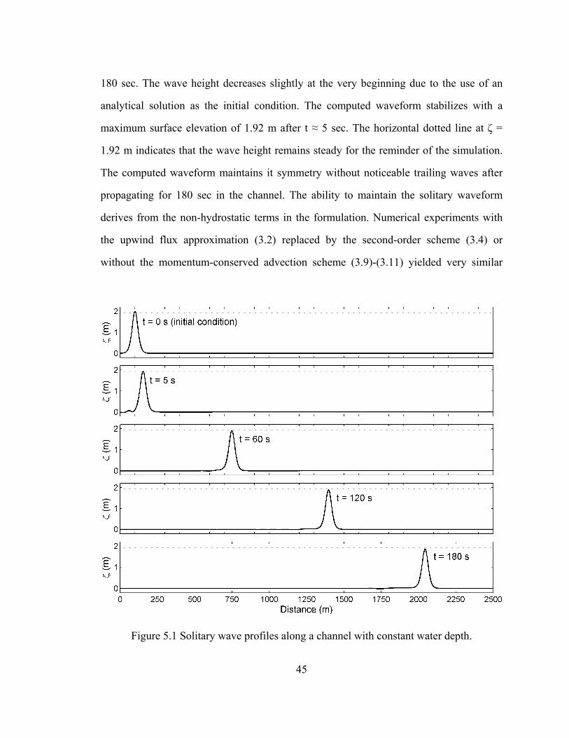
180 sec. The wave height decreases slightly at the very beginning due to the use of an
analytical solution as the initial condition. The computed waveform stabilizes with a
maximum surface elevation of 1.92 m after t ≈ 5 sec. The horizontal dotted line at ζ =
1.92 m indicates that the wave height remains steady for the reminder of the simulation.
The computed waveform maintains it symmetry without noticeable trailing waves after
propagating for 180 sec in the channel. The ability to maintain the solitary waveform
derives from the non-hydrostatic terms in the formulation. Numerical experiments with
the upwind flux approximation (3.2) replaced by the second-order scheme (3.4) or
without the momentum-conserved advection scheme (3.9)-(3.11) yielded very similar
Figure 5.1 Solitary wave profiles along a channel with constant water depth.
45

46
results, which are not presented here for brevity. Refinement of the computational grid,
however, diminished the initial reduction of the wave height, confirming that as a
numerical artifact.
The numerical experiment of solitary wave propagation also provides a critical test for
the grid-nesting scheme. The model must accurately transfer the flow kinematics and
non-hydrostatic pressure and balance the nonlinear and dispersive effects across nested
grids of different resolution to maintain the solitary waveform. In the second numerical
experiment, a solitary wave propagates in a 45 m long, 25 m wide, and 0.5 m deep
channel with two levels of nested grids. The initial conditions correspond to a 0.05-m
high solitary wave at x = 7.5 m. Figure 5.2 shows a sequence of the computed waveforms
in their original resolution as the solitary wave propagates through the inner grid. The
numerical experiment uses 20-cm resolution for the level-1 outer grid and 4-cm for the
level-2 inner grid. The inner grid configuration allows testing of solitary wave
propagation at different directions with respect to the inter-grid boundary. The solitary
wave enters the level-2 grid around t = 2.5 sec and leaves at 15.0 sec. Even though the
inter-grid boundary is set oblique to the wave direction, the solitary wave passes through
the nested-grid smoothly with invisible surface disturbance and leaves no residual
oscillation near the inter-grid boundary, thereby verifying the capability of the grid-
nesting scheme for dispersive wave propagation.

Figure 5.2 Propagation of solitary wave across two levels of nested grids in a channel of constant depth. Dark blue indicates the level-1 grid and light blue denotes the level-2 grid results.
47

5.2 Sinusoidal Wave Propagation over a Bar
Beji and Battjes (1993) and Luth et al. (1994) conducted a laboratory experiment to
examine sinusoidal wave propagation over a submerged bar. Figure 5.3(a) shows the
experiment setup in a 37.7-m long, 0.8-m wide, and 0.75-m high wave flume. A
hydraulically driven, piston-type wave generator is located at the left side of the flume
and a 1:25 plane beach with coarse material is placed at the right side to serve as a wave
absorber. The submerged trapezoidal bar is 0.3 m high with front slope of 1:20 and lee
slope of 1:10. The computational domain in Figure 5.3(b) is 35 m long and 0.4 m deep
and is discretized with Δx = Δy = 1.25 cm and Δt = 0.01 sec. Surface roughness is
unimportant in this experiment and a Manning’s coefficient n = 0.0 is used. We consider
the test case with 1-cm incident wave amplitude and 2.02-sec wave period that
(a) 4 5 6 7 8 9 10 11
h= 40 cm
1:20 1:10 1:25
h= 10 cm
Wave absorber
35 m
6 m 6 m 2 m 3 m 2 m 16 m
(b) 4 5 6 7 8 9 10 11
Figure 5.3 Definition sketch of wave transformation over a submerged bar. (a) Laboratory setup. (b) Numerical setup. , gauge locations.
48

corresponds to the water depth parameter kh = 0.67. The incident sinusoidal waves are
generated at the left boundary and the radiation boundary condition is imposed on the
right. The free surface elevations are output at eight gauge locations over and behind in
accordance to the laboratory experiment.
Figure 5.4 shows the computed and recorded waveforms at the eight gauges. The
measured data at gauge 4 provides a reference for adjustment of the timing of computed
waveforms. The present model with either the upwind flux approximation (3.2) or the
Figure 5.4 Comparison of computed and measured free surface elevations over and behind a submerged bar. , laboratory data of Beji and Battjes (1993); ⎯⎯ (red), non-hydrostatic model with upwind flux scheme; - - - - (blue), second order scheme.
49

50
second-order scheme (3.4) in the continuity equation reproduces the wave transformation
at gauge 4 over the front slope and at gauge 5 immediately behind the front slope. The
computed results maintain good agreement with the laboratory data at gauges 6 to 8 over
the crest and the lee slope, where the waveform undergoes significant transformation
with high frequency dispersion. Noticeable discrepancies arise between the computed and
recorded waveforms over the flat bottom behind the bar, where the laboratory data from
gauges 9 to 11 shows evidence of super-harmonics around 1 sec and 0.67 sec periods,
which correspond to kh = 1.7 and 3.6, respectively. The third-order waves with kh = 3.6
behind the bar are the source of dispersion errors as inferred from Figure 2.2.
Overall, the upwind flux approximation (3.2) and the second-order scheme (3.4) in the
present model provide the same or slightly better results compared to Stelling and
Zijlema (2003) and Walters (2005). The present and previously computed waveforms are
almost identical, when the depth-integrated models are within the applicable range of the
non-hydrostatic approximation. The high-frequency waves behind the bar exceed the
applicable range of a weakly dispersive model. Under these critical conditions, the
second-order scheme provides larger wave amplitudes, which can be seen at gauges 7 to
10, especially at gauge 9. This alludes to the importance of the upwind flux
approximation in maintaining numerical stability of the model especially when
implemented outside its applicable range.
5.3 N-wave Transformation and Runup
Matsuyama and Tanaka (2001) conducted a laboratory study at the Central Research
Institute for Electric Power Industry (CRIEPI) to investigate the nearshore wave
dynamics of the 1993 Hokkaido Nansei-Oki Tsunami. Eyewitness reported initial
withdraw of the water followed by a large tsunami wave at the coast causing 31.7 m of

51
runup near Monai Valley, Japan. Such observations fit the description of the leading-
depression N-wave, which is often used in laboratory studies of tsunami impact close to
the source. The CRIEPI wave flume is 205 m long, 3.4 m wide, and 6 m high with
reflective sidewalls and a hydraulic, piston-type wave maker capable of generating N-
waves. The 1:400-scale coastal relief model around Monai Valley was constructed of
painted plywood and installed approximately 140 m from the wave generator. The initial
N-wave was relatively long with a very gentle profile and dispersed into a series of short-
period waves over the coastal relief model in the experiment. The measured water level
data and runup from the experiment allow validation of the present grid-nesting scheme
in describing generation of dispersive waves across inter-grid boundaries.
The grid-nesting scheme describes wave dynamics at resolution compatible with the
physical process and spatial scale for optimization of computational efficiency. Figure
5.5(a) shows the numerical experiment setup over the 5.475-m long and 3.4-m wide relief
model at 1.4 cm resolution (5.6 m full scale). The level-1 grid covers the entire panel at
2.5 cm resolution (10 m full scale) and the level-2 grid at 1.25-cm resolution (5 m full
scale) provides a more detailed description of the nearshore wave processes in the
outlined area from Monai Valley to the 0.035-m (14-m full scale) depth contour. A
Manning’s coefficient n = 0.012 describes the surface roughness of the painted plywood
model (Chaudhry, 1993). Figure 5.5(b) shows the input N-wave profile at the left
boundary with 0.135 m (54 m full scale) water depth. The incident waves shoal over a
plane slope before refracting and diffracting around a small island on a shallow bank.
Figure 5.6(a) shows very good agreement of the computed surface elevations with the
laboratory measurements at three gauges behind the island. The model reproduces the
small-amplitude dispersive waves generated by reflection from the coast with a minor

Figure 5.5 Input data for Monai Valley experiment. (a) Level-1 computational domain. (b) Initial wave profile. , gauge locations; ⎯⎯, Level-2 computational domain; ⎯⎯ (black), topography contours at 0.0125-m intervals; - - - - (grey), bathymetry contours at 0.0125-m intervals; ⎯⎯, initial profile.
phase lag, but the results are better than those from the extended Boussinesq model of
Nwogu (2008) in dispersive wave estimation. We recomputed the results with a uniform
grid at the same 1.25-cm resolution (5 m full scale) as the level-2 nested grid over the
entire domain and obtained almost identical results as shown in Figure 5.6(b).
52

Figure 5.6 Time series of surface elevation at gauges in Monai Valley experiment. (a) Comparison of measurements with nested-grid solution. (b) Comparison of nested and uniform grid solutions. ⎯⎯ (black), laboratory data of Matsuyama and Tanaka (2001); ⎯⎯ (red), grid-nesting solution; - - - - (blue), uniform grid solution.
Table 5.1. Recorded runup for the six trials from Matsuyama and Tanaka (2001).
Trial No. Maximum y = 2.2062 m y = 2.32 m
Rmax (cm) (Full scale in m) R (cm) (Full scale in m) R (cm) (Full scale in m)
209_105 8.75 (35.0) 5.25 (21.0) 5.25 (21.0) 209_106 9.00 (36.0) 5.75 (23.0) 5.50 (22.0) 209_107 8.00 (32.0) 5.50 (22.0) 5.50 (22.0) 210_101 9.00 (36.0) 6.50 (26.0) 5.75 (23.0) 210_102 10.00 (40.0) 6.75 (27.0) 5.75 (23.0) 210_103 9.00 (36.0) 6.50 (26.0) 5.75 (23.0)
mean 8.97 (35.8) 6.04 (24.2) 5.58 (22.3)
53
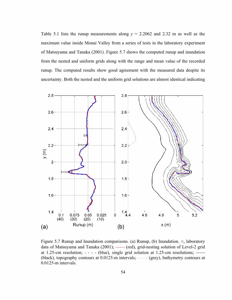
Table 5.1 lists the runup measurements along y = 2.2062 and 2.32 m as well as the
maximum value inside Monai Valley from a series of tests in the laboratory experiment
of Matsuyama and Tanaka (2001). Figure 5.7 shows the computed runup and inundation
from the nested and uniform grids along with the range and mean value of the recorded
runup. The computed results show good agreement with the measured data despite its
uncertainty. Both the nested and the uniform grid solutions are almost identical indicating
Figure 5.7 Runup and Inundation comparisons. (a) Runup, (b) Inundation. , laboratory data of Matsuyama and Tanaka (2001); ⎯⎯ (red), grid-nesting solution of Level-2 grid at 1.25-cm resolution; - - - - (blue), single grid solution at 1.25-cm resolutions; ⎯⎯ (black), topography contours at 0.0125-m intervals; - - - - (grey), bathymetry contours at 0.0125-m intervals.
54

55
the proposed grid-nesting scheme appropriately transfers information across the inter-grid
boundary and provide results of the same accuracy as the uniform grid solution. The
minor discrepancies near the inter-grid boundaries are due to transition of the bathymetry
from the outer to the inner grid. Comparisons of the surface elevation, runup, and
inundation from the Moani Valley experiment verify the proposed gird-nesting scheme in
handling dispersive wave and runup processes over complex nearshore bathymetry and
topography.

CHAPTER 6
WAVE BREAKING AND RUNUP
NEOWAVE uses a momentum conservation scheme to model wave breaking as bores or
hydraulic jumps without the use of artificial dissipation models. The scheme, which does
not require calibration, accounts for energy dissipation across flow discontinuities. The
benchmark laboratory experiments of solitary wave transformation over a plane beach
and a conical island involve energetic breaking waves in the runup and drawdown
processes. Numerical experiments of these tests provide a systematic examination of the
model performance with and without the momentum conservation scheme.
6.1 Solitary Wave Runup on a Plane Beach
Hall and Watts (1953), Li and Raichlen (2002), and Synolakis (1987) conducted series of
laboratory experiments for solitary wave transformation and runup on a plane beach.
These experiments, which cover a wide range of non-breaking and breaking waves, have
become an accepted test case for validation of runup models (Titov and Synolakis, 1995;
Lynett et al., 2002; Li and Raichlen, 2002; Wei et al., 2006; and Roeber et al., 2010).
Figure 6.1 provides a schematic of the experiments with A indicating the incident solitary
56
A
h
L / 2
R
β
Figure 6.1 Definition sketch of solitary wave runup on a plane beach.

wave height, β the beach slope, and R the runup. Following Titov and Synolakis (1995),
the solitary wave is initially at a half wavelength from the toe of the beach in the
numerical experiment. The approximate wavelength of a solitary wave is give by
⎟⎟⎠
⎞⎜⎜⎝
⎛=
05.01harccos2
kL (6.1)
in which the wave number 33 / 4k A= h . In the numerical experiment, we use Δx/h =
0.125 and a Courant number Cr = 0.2. Surface roughness becomes important for runup
over gentle slopes and a Manning’s coefficient n = 0.01 describes the surface condition of
the smooth glass beach in the laboratory experiments (Chaudhry, 1993).
Titov and Synolakis (1995) presented a series of surface profiles with a beach slope of
1:19.85 and solitary wave heights of up to A/h = 0.3. Initial testing with this experiment
reiterates and furthers the findings from the experiments of sinusoidal wave
transformation in Section 5.2. The upwind flux approximation of the surface elevation is
essential in maintaining stability of the depth-integrated non-hydrostatic model,
especially when flow discontinuities associated with breaking waves and hydraulic jumps
develop. The second-order scheme produces spurious waves near the discontinuity that
lead to development of instabilities in most of the tests. As a result, this test case uses the
upwind flux approximation in the model and examines the treatment of the advective
terms in the momentum equations by presenting results with and without the momentum-
conserved advection approximation (3.9)-(3.11). When this scheme is off, the advective
terms are computed directly from (3.3).
Figure 6.2 shows a comparison of the measured profiles with the two sets of numerical
results for the test case with the solitary wave height A/h = 0.3. The laboratory data shows
wave breaking between t(g/h)½ = 20 and 25 as the solitary wave reaches the beach and
development of a hydraulic jump at t(g/h)½ = 50 when the water recedes from the beach.
57

Figure 6.2 Surface profiles of a solitary wave transformation on a 1:19.85 plane beach with A/h = 0.3. , laboratory data of Titov and Synolakis (1995); ⎯⎯ (red), non-hydrostatic model with momentum-conserved advection; - - - - (blue), without momentum-conserved advection.
Both numerical solutions show very good agreement with the laboratory data as the
solitary wave shoals to its maximum height at t(g/h)½ = 20. The momentum-conserved
advection scheme reproduces the subsequent wave breaking without the use of
predefined criteria and matches the surface elevation and runup on the beach. Without the
momentum-conserved advection, the model cannot reproduce the surface profile at
58

59
t(g/h)½ = 25 immediately after wave breaking and underestimates the surface elevation on
the beach and eventually the runup. Both solutions describe the surface elevation
reasonably well during the drawdown process. A minor discrepancy on the location of the
hydraulic jump occurs around the peak of the return flow at t(g/h)½ = 55. The finite
volume model of Wei et al. (2006) also produces a similar discrepancy with the
laboratory data. This may be attributed to the three-dimensional flow structure that is not
amenable to depth-integrated solutions. The agreement resumes as the speed of the return
flow decreases demonstrating the resilience of the model.
Figure 6.3 shows the computed and measured runup R/h as a function of the solitary
wave height A/h for beach slopes of 1:5.67, 1:15, and 1:19.85. The measured data shows
a bilinear distribution with the two branches representing the non-breaking and breaking
regimes separated by a transition. Figure 6.3(a) shows good agreement of the two
solutions with the laboratory data for non-breaking and breaking wave runup on the
1:5.67 slope. This steep slope most likely produces surging wave breakers that are
amenable to non-hydrostatic models without special treatments to the momentum
equations. Wave breaking becomes more energetic and the resulting surface elevation
becomes discontinuous as the beach slope decreases. In Figure 6.3(b) and 6.3(c), the
computed runup from the momentum-conserved advection approximation shows
excellent agreement with the laboratory data for both non-breaking and breaking waves.
Without the momentum-conserved advection, the solution reproduces the runup in the
non-breaking and transition regimes, but underestimates the measured runup for breaking
waves with A/h > 0.1. This shows that implementation of the momentum-conserved
advection scheme in a non-hydrostatic model can capture discontinuous flows associated
with energetic wave breaking and describe the subsequent runup on the beach without an
empirical dissipation term.

Figure 6.3 Solitary wave runup on a plane beach as a function of incident wave height. (a) 1/5.67 (Hall and Watts, 1953). (b) 1/15 (Li and Raichlen, 2002). (c) 1/19.85 (Synolakis, 1987). , laboratory data; ⎯⎯ (red), non-hydrostatic model with momentum-conserved advection; - - - - (blue), without momentum-conserved advection.
60

6.2 Solitary Wave Runup on a Conical Island
Briggs et al. (1995) conducted a large-scale laboratory experiment to investigate solitary
wave runup on a conical island. The collected data has become a standard for validation
of runup models (Liu et al., 1995a; Titov and Synolakis, 1998; Chen et al., 2000; Lynett
et al., 2002; and Wei et al., 2006). Figure 6.4 shows a schematic of the experiment. The
basin is 25 m by 30 m. The circular island has the shape of a truncated cone with
diameters of 7.2 m at the base and 2.2 m at the crest. The island is 0.625 m high and has a
side slope of 1:4. The surface of the island and basin has a smooth concrete finish. A
27.4-m long directional spectral wave maker, which consists of 61 paddles, generates
solitary waves for the experiment. Wave absorbers at the three sidewalls reduce reflection
in the basin.
(a)
30 m
25 m
180º
90º
0º
C B
9 16
22
270º 6
A
2
13 m
15 m
(
61
Figure 6.4 Schematic sketch of the conical island experiment. (a) Perspective view. (b) Side view (center cross section). , gauge locations.
A B C 6 9 22 30.5 cm
1.1 m b) 3.6 m 2
32.0 cm

62
The experiment covers the water depths h = 0.32 and 0.42 m and the solitary wave
heights A/h = 0.05, 0.1 and 0.2. The present study considers the smaller water depth h =
0.32 m, which provides a more critical test case for the non-hydrostatic model. In the
computation, the solitary wave is generated from the left boundary with the measured
initial wave heights of A/h = 0.045, 0.096, and 0.181. These measured wave heights,
instead of the target wave heights A/h = 0.05, 0.1, and 0.2 in the laboratory experiment,
better represent the recorded data at gauge 2 and thus the incident wave conditions to the
conical island. The radiation condition is imposed at the lateral boundaries to model the
effects of the wave absorbers. We use Δx = Δy = 5 cm, Δt = 0.01 sec, and a Manning’s
roughness coefficient n = 0.016 for the smooth concrete finish according to Chaudhry
(1993). Since wave breaking occurred during the laboratory experiment, we use the
upwind flux approximation in the computation to model the processes.
The solution obtained with the momentum-conserved advection scheme provides an
illustration of the solitary wave transformation around the conical island. Figure 6.5
shows the results when the wave reaches the maximum elevation on the front face of the
island and 2 sec afterward. Because the celerity increases with the wave height, the
arrival time of the solitary wave is about 1.4 sec apart for the wave height range
considered. The three test cases show similar wave processes despite the difference in
amplitude. The results show refraction and trapping of the solitary wave over the island
slope. The left panels of Figure 6.6 shows the trapped waves from the two sides
superpose with the diffracted wave on the leeside of the island. Wave breaking occurs
locally for A/h = 0.096 and everywhere around the island for A/h = 0.181 according to
Titov and Synolakis (1998). This reduces the subsequent runup on the leeside of the
island. The right panels shows the free surface 2 sec later when the trapped waves have
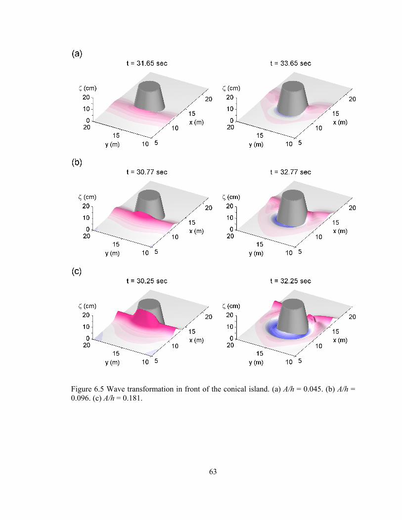
Figure 6.5 Wave transformation in front of the conical island. (a) A/h = 0.045. (b) A/h = 0.096. (c) A/h = 0.181.
63

Figure 6.6 Wave transformation on the leeside of the conical island. (a) A/h = 0.045. (b) A/h = 0.096. (c) A/h = 0.181.
64

65
passed each other and continue to wrap around to the front. Munger and Cheung (2008)
reported similar trapped waves around the Hawaiian Islands generated by the 2006 Kuril
Islands Tsunami.
The free surface is rather smooth with indistinguishable frequency dispersion before the
wave wraps around the island. As the solitary wave travels down the basin, high-
frequency dispersive waves become evident around the island especially on the leeside.
The test case with A/h = 0.181 provides a vivid depiction of the generation and
propagation of the dispersive waves. Figures 6.5(c) and 6.6(c) show the generation of the
first group of dispersive waves as the trapped waves wrap around the island and collide
on the leeside. After the collision, the second group of dispersive waves is generated due
to energy leakage from the two trapped waves that continue to wrap around to the front.
The interaction of the first and second groups of dispersive waves generates a mesh-like
wave pattern behind the island. These high-frequency dispersive waves provide an
explanation for the 3 to 5-min edge waves recorded on the south shore of Oahu after the
2006 Kuril Islands Tsunami that a nonlinear shallow-water model cannot reproduce even
with a 10-m computational grid (Bricker et al., 2007).
A number of gauges recorded the transformation of the solitary wave around the conical
island. Figure 6.7 shows the time series of the solutions with and without the momentum-
conserved advection scheme and the measured free surface elevations at selected gauges.
With reference to Figure 6.4, gauges 2 and 6 are located in front of the island and 9, 16,
and 22 are placed just outside the still waterline around the island. These gauges provide
sufficient coverage of the representative wave conditions in the experiment. The
measured data at gauge 2 provides a reference for adjustment of the timing of the
computed waveforms. Both solutions show excellent agreement with the measured time

Figure 6.7 Time series of surface elevations at gauges around a conical island. (a) A/h = 0.045. (b) A/h = 0.096. (c) A/h = 0.181. , laboratory data from Briggs et al. (1995); ⎯⎯ (red), non-hydrostatic with momentum-conserved advection; - - - - (blue), without momentum-conserved advection.
series including the depression following the leading wave that was not adequately
reproduced in previous studies. The momentum-conserved advection scheme reasonably
describes the phase of the peak, but slightly overestimates the leading wave amplitude at
gauges 9 and 22 as the wave height increases. Without the momentum conservation, the
model generally reproduces the leading wave amplitude except at gauge 22 with A/h =
0.181, where the model fails to fully capture the energetic breaking wave on the leeside
of the island. This reiterates the importance of the momentum-conserved advection
scheme in capturing breaking waves.
66

Figure 6.8 shows comparisons of the measured and computed inundation and runup
around the conical island. Both solutions are almost identical and show good agreement
with the laboratory data. The momentum-conserved advection produces better
estimations at the lee flank of island around 90º ~ 160º, where the runup is lowest. For
the results presented in Figures 6.7 and 6.8, both solutions are comparable or slightly
better than the extended Boussinesq solutions of Chen et al. (2000) and Lynett et al.
(2002) that use empirical relations with adjustable coefficients to describe wave breaking.
Most of the previous studies neglected friction in this numerical experiment (Liu et al.,
1995a; Titov and Synolakis, 1998; Chen et al., 2000; and Lynett et al., 2002). A test of
the model with n = 0.0 gave very similar results as n = 0.016. As pointed out in Liu et al.
(1995a), the computed results are not sensitive to the surface roughness coefficient due to
the steep 1:4 slope of the conical island. The overall agreement between the computed
results and laboratory data indicates the capability of the present model to estimate wave
transformation, breaking, and inundation in the two horizontal dimensions.
Figure 6.8 Inundation and runup around a conical island. (a) A/h = 0.045. (b) A/h = 0.096. (c) A/h = 0.181. , laboratory data from Briggs et al. (1995); ⎯⎯ (red), non-hydrostatic model with momentum-conserved advection; - - - - (blue), without momentum-conserved advection.
67
68
CHAPTER 7
THE 2009 SAMOA TSUNAMI
The objective behind the development of NEOWAVE is to have a model that can
describe the tsunami evolution process from generation, propagation to runup with due
consideration to dynamic seafloor deformation, wave dispersion, wave breaking, and
bore propagation at appropriate resolution. The 2009 Samoa Tsunami affected regions
with steep and irregular offshore bathymetry as well as extended shallow fringing reefs.
The well-recorded event provides a critical test case to validate NEOWAVE for real-field
tsunami modeling.
7.1. Model Setup
The Samoa earthquake occurred near the Tonga trench on 29 September 2009 at 17:48:10
UTC. The US Geological Survey (USGS) determined the epicenter at 15.509°S
172.034°W and estimated the moment magnitude Mw of 8.1. Figure 7.1 shows the
rupture configuration and the locations of the water-level stations in the region. The main
energy of the resulting tsunami propagated toward Tonga and American Samoa. The tide
gauge in Pago Pago Harbor, Tutuila (American Samoa), and the DART buoys 51425,
51426, and 54401 surrounding the rupture area recorded clear signals of the tsunami. The
tsunami arrived at mid tide and produced maximum runup of 17.6 m and detrimental
impact on Tutuila. The rugged, volcanic island sits on a shallow shelf of less than 100 m
deep covered by mesophotic corals (Bare et al., 2010). The insular slope is steep with
gradients up to 1:2 on the west side and drops off abruptly to over 3000 m depth in the
surrounding ocean. Several field survey teams recorded and documented the tsunami
runup and inundation around Tutuila and provided useful data for model validation (Fritz
et al., 2009; Koshimura et al., 2009; and Jaffe et al., 2010).

Figure 7.1 Bathymetry and topography in the modeled region for the 2009 Samoa Tsunami. (a) Level-1 computational domain. (b) Close-up view of rupture configuration and Samoa Islands. ·········, rupture area; (red), epicenter; (white), water-level stations.
We reconstruct the 2009 Samoa Tsunami from its generation at the earthquake source to
runup at Pago Pago Harbor with four levels of nested grids. Figure 7.1(a) shows the
coverage of the level-1 grid, which spreads across the south-central Pacific at 1-min (≈
1800-m) resolution. An open boundary condition allows radiation of tsunami waves away
from the domain. Figure 7.2 shows the original and the smoothed bathymetry at the next
three levels. The level-2 grid covers American Samoa down to the 4000-m depth contour
at 7.5-sec (≈ 225-m) resolution to capture wave transformation around the island group.
The level-3 grid resolves the shelf and steep bathymetry down to the 1500-m depth
contour around Tutuila at 1.5 sec (~ 45 m) and provides a transition to the level-4 grid,
which covers Pago Pago Harbor at 0.3 sec (~9 m) resolution for computation of
inundation as well as tide gauge signals. A Manning’s coefficient n = 0.035 describes the
69

Figure 7.2 Coverage of levels 2, 3, and 4 computational domain. (a) Original bathymetry and topography. (b) Smoothed data with depth-dependent Gaussian function. , Pago Pago tide station.
surface roughness in the near-shore seabed with fringing reefs according to Bretschneider
et al. (1986). The momentum-conserved advection scheme is used at the level-4 grid,
where flow discontinuities associated with wave breaking and bore formation would
otherwise cause volume loss and numerical dissipation.
70

71
The digital elevation model is derived from a blended dataset of multiple sources. The
0.5-min (≈ 900-m) General Bathymetric Chart of the Oceans (GEBCO) from the British
Oceanographic Data Centre (BODC) provides the bathymetry for Pacific Ocean. The
Coastal Relief Model from National Geophysical Data Center (NGDC) covers the
American Samoa region and Tutuila at 3 and 0.3333 sec (~90 and 10 m) resolution
respectively. Embedded in the NGDC dataset are multibeam and satellite measurements
around Tutuila and high-resolution LiDAR (Light Detection and Ranging) survey data at
Pago Pago Harbor. We have converted the datasets to reference the WGS 84 datum and
the mean-sea level (MSL). The Generic Mapping Tools (GMT) interpolates the data to
produce the computational grids. The original data in Figure 7.2(a) shows fine details of
the seafloor. Smoothing of the bathymetry data is sometime necessary to ensure a
converging solution from the non-hydrostatic model. Figure 7.2(b) shows the processed
data with the depth-dependent Gaussian function. The proposed scheme removes fine
features in deep water that should have little effect on tsunami propagation, but retains
the near-shore details important for inundation computation.
7.2 Tsunami Generation
The present non-hydrostatic model utilizes the vertical velocity to describe dispersive
waves. This also facilitates modeling of tsunami generation through dynamic deformation
of the seafloor due to earthquake rupture. USGS analyzed the rupture processes of the
2009 Samoa Earthquake using the finite fault inverse algorithm of Ji et al. (2002) and
estimated the fault parameters such as depth, orientation, and slip over 420 subfaults of 6
km by 6 km each. The analysis provides the rupture initiation time and rise time for 249
subfaults with seismic moment of over 1025 dyne-cm.
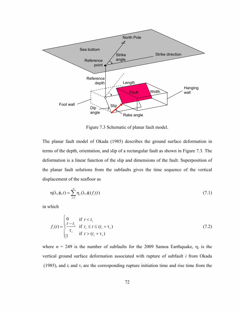
Reference point
Slip
North Pole
Strike angle
Reference depth Length
Rake angle
Dip angle
Strike direction
Width
Sea bottom
Hanging wall
Foot wall
Fault
Figure 7.3 Schematic of planar fault model.
The planar fault model of Okada (1985) describes the ground surface deformation in
terms of the depth, orientation, and slip of a rectangular fault as shown in Figure 7.3. The
deformation is a linear function of the slip and dimensions of the fault. Superposition of
the planar fault solutions from the subfaults gives the time sequence of the vertical
displacement of the seafloor as
∑=
φλη=φληn
iii tft
1)(),(),,( (7.1)
in which
)(if)(if
if
1
0)(
ii
iii
i
i
ii
ttttt
tttt
tfτ+>
τ+≤≤<
⎪⎪⎩
⎪⎪⎨
⎧
τ−
= (7.2)
where n = 249 is the number of subfaults for the 2009 Samoa Earthquake, ηi is the
vertical ground surface deformation associated with rupture of subfault i from Okada
(1985), and ti and τi are the corresponding rupture initiation time and rise time from the
72

73
USGS finite fault solution. The source time function (7.2) defines a linear motion of the
slip at each subfault to approximate the rupture process (Irikura, 1983).
The USGS finite fault solution shows an average rise time of 3.4 sec for the subfault
movement and a rupture duration of 94 sec for the entire event. Figure 7.4 shows the
rupture, seafloor deformation, and free surface elevation during the tsunami generation
process. The rupture starts at the epicenter located on the north side of the fault and
propagates toward south. Despite the granularity of the finite fault model, the seafloor
deformation is rather continuous due to the depth of the fault below the ground surface.
The generation of tsunami waves from the seafloor deformation occurs simultaneously
with the propagation of the energy away from the source. In addition, the present
approach transfers both the kinetic and potential energy from the seafloor to the water.
This results in different seafloor deformation and surface wave patterns in contrast to the
static deformation approach. The earthquake releases most of the energy in 30 sec and the
subsequent rupture has minimal effect on the seafloor deformation. By the end of the
rupture at t = 94 sec, the tsunami has propagated over a considerable distance with a
leading depression toward the Samoa Islands.

Figure 7.4 Time sequence of rupture and tsunami generation. (a) Slip distribution. (b) Sea floor deformation. (c) Surface elevation. ⎯⎯, uplift contours at 0.2-m intervals; - - - -, subsidence contours at 1.0-m intervals.
74

7.3 Surface Elevation and Runup
Tsunami energy propagation is directional with the majority perpendicular to the fault-
line. Figure 7.5 shows the tsunami wave amplitude over South Central Pacific with a
maximum value of 1.8 m over the deep ocean. The main energy propagates toward Tonga
in the west and American Samoa in the east with significant impacts to Tutuila, where the
tide gauge in Pago Pago Harbor recorded a strong signal of the tsunami. The three DART
buoys, which are located off the main energy beams, also recorded clear signals.
Figure 7.5 Maximum surface elevation for the 2009 Samoa Tsunami. (white), water level stations; (red), epicenter of the 2009 Samoa Earthquake; ·········, rupture area.
75

Figure 7.6 Wave propagation and inundation at inner Pago Pago Harbor. ⎯⎯ (black), coastline; ⎯⎯ (grey), contours at 2.5-m intervals.
Pago Pago Harbor is an L-shape embayment with fringing reefs along its shores. The
reefs converge at the west end of the harbor forming an extended shallow flat favorable
to bore or hydraulic jump formation (Roeber et al., 2010). The water over the 1000-m
long reef flat is approximately 10 m deep and the depth increases to 30 m over a distance
76

77
of 500 m from the reef edge. Figure 7.6 shows a series of the computed surface elevation
in the inner harbor that corroborates witness accounts during the first wave (Koshimura et
al., 2009). The water begins to withdraw approximately 20 min after the earthquake
exposing the shallow reef flats along the shores. The first positive wave, which arrives
shortly afterward, reaches a surface elevation of 2 m in the inner harbor and floods the
low-lying coastal areas on the north and south sides. The wave develops a sharp surface
gradient over the reef flat around t = 26 min and transforms into a surge as it hits dry land
reaching a maximum elevation of 8.14 m and producing extensive damage in the area. A
hydraulic jump develops at the reef edge around t = 31.0 min as the floodwater returns to
the harbor. The wave retreats faster than the receding floodwater resulting in
accumulation of water on land and a waterfall over the reef edge until the next wave
arrives.
Figure 7.7 shows a comparison of the recorded and computed waveforms and spectra at
the Pago Pago tide gauge and the three DART buoys. The computed results show good
agreement of the arrival time, amplitude, and frequency content with the measurements.
The model reproduces the initial negative wave at the tide gauge and captures the distinct
11 and 18-min oscillations at Pago Pago Harbor. Some discrepancies of the initial
waveforms are evident at the DART buoys. The model over-estimates the amplitude of
the leading depression at DART 51425 and cannot reproduce the polarity at DART
51426 and 54401. However, the amplitude recorded at these buoys is less than 4% of the
1.8-m maximum amplitude in the open ocean to the east of the source. The error might be
attributed to the details of the source mechanism or the assumed location and predefined
strike and dip angles of fault in the USGS finite fault solution that become noticeable off
the main energy beams. The overall source mechanism is deemed accurate as it
reproduces the observations and strong tsunami signals at Pago Pago Harbor. In fact, the

model results at DART 51426 and 54401 reproduce the high-amplitude reflected waves
from Tutuila arriving at 1.6 hours and 3.2 hours after the earthquake.
Pago Pago Harbor is 50 m deep, while the 100-m deep outside embayment is sheltered by
barrier reefs along the edge of the insular shelf as shown in Figure 7.8(a). The
configuration of the harbor and embayment is prone to trapping of long waves and the
two distinct peaks in the amplitude spectrum are indicative of resonance. Following the
method of Munger and Cheung (2008) based on Fast Fourier Transform, we extract the
Figure 7.7 Time series and spectra of surface elevations at water level stations. ⎯⎯ (black), recorded data; ⎯⎯ (red), computed data.
78

Figure 7.8 Detailed bathymetry and resonance modes around Pago Pago Harbor. (a) bathymetry. (b) First mode at 18 min. (c) Second mode at 11 min. (d) Third mode at 9.6 min. ⎯⎯ (grey), depth contours at 25-m intervals; - - - - (grey), depth contours at 500-m intervals.
79

80
oscillation modes of the modeled tsunami waves. The spectral analysis depicts three
resonance modes at 9.7, 11, and 18 min period in Pago Pago Harbor that are plotted in
Figure 7.8. The first resonance at 18 min extends from the embayment into Pago Pago
Harbor. The resonance mode shows a node along the edge of the insular shelf and an
antinode at the tip of the harbor. The second resonance mode at 11 min covers the same
region with two nodes located at the harbor entrance and the edge of the insular shelf.
The third mode at 9.7 min, with a relatively lower energy level in this event, has an
additional node in the outside embayment. The combined effect of the first two resonance
modes provides an explanation for the significant inundation and property damage
despite the well-sheltered location of the harbor.
The results presented so far have been based on the smoothed bathymetry in Figure 7.2
(b). We compute the runup and inundation at level 4 with both the smoothed and original
bathymetry to assess the effectiveness of the depth-dependent smoothing scheme. Figure
7.9 compares the computed runup and inundation around Pago Pago Harbor with the
measurements from Fritz et al. (2009) and Koshimura et al. (2009). The two sets of
computed runup results are almost identical thereby verifying the proposed smoothing
scheme that serves to improve model convergence without appreciable alteration of the
model results. The smoothing of the bathymetry results in a 10% reduction of the number
of iterations in the non-hydrostatic solver that is relatively minor because of the lack of
small-scale, steep bottom features in the level-4 grid. In some situations, smoothing is
necessary to obtain converging non-hydrostatic solutions. The model reproduces the
overall pattern of the runup along the shorelines. The minor discrepancies between the
computed results and measurements are primarily due to errors in topographic data and
the difficulties in modeling inundation in the built environment around Pago Pago Harbor.
The large runup at the tip and low values in the outer harbor show strong correlation with

the three resonance modes. Such oscillation patterns also provide an explanation of the
local amplification and the disparate property damage along the coastlines of Tutuila.
Figure 7.9 Runup and inundation at inner Pago Pago Harbor. ⎯⎯ (white), recorded inundation; (white): recorded runup; (blue): recorded flow depth plus land elevation; ⎯⎯ (red), solution with smoothed bathymetry; - - - - (blue), solution with non-smoothed bathymetry; ⎯⎯ (black), coastline; ⎯⎯ (grey), depth contours at 10-m intervals; - - - - (black), computed runup projection.
81

82
CHAPTER 8
CONCLUSIONS AND RECOMMENDATIONS
This dissertation has demonstrated the versatility and robustness of a depth-integrated,
non-hydrostatic model for tsunami research and impact assessment. The key feature in
the formulation is the decomposition of the pressure into hydrostatic and non-hydrostatic
components and the introduction of a linear vertical velocity in conjunction with the non-
hydrostatic pressure. This allows modeling of dynamic seafloor deformation in tsunami
generation and wave dispersion effects during the evolution processes. The hydrostatic
component is equivalent to a nonlinear shallow-water model with an explicit scheme. An
implicit scheme provides the non-hydrostatic pressure through the three-dimensional
continuity equation. The semi-implicit, finite difference model describes flow
discontinuities associated with breaking waves and bore development using the
momentum-conserved advection scheme. An upwind flux scheme extrapolates the free
surface elevation instead of the flow depth in the computation of the continuity equation
and the momentum-conserved advection to improve model stability. A depth-dependent
Gaussian function improves the convergent rate in the implicit solution of the non-
hydrostatic pressure.
The lower-order spatial derivatives in the governing equations allow implementation of a
grid-nesting scheme for the shock-capturing, dispersive model. A two-way nesting
scheme exchanges the horizontal velocity, surface elevation, and non-hydrostatic
pressure between an inner and an outer grid at every outer grid time step. The use of both
the velocity and surface elevation in the nesting scheme is necessary to implement the
momentum-conserved advection scheme as well as the upwind flux scheme across the
inter-grid boundaries. A Dirichlet boundary condition for the non-hydrostatic pressure
ensures wave dispersion is continuous across the inter-grid boundaries. This nested-grid

83
enables the use of non-rectangular computational domains that can adapt to bathymetric
contours and features for optimization of computational time. The model in the spherical
coordinate system accounts for the earth’s curvature in basin-wide tsunami propagation
and yet is flexible enough to describe detailed wave transformation and runup at a coastal
region.
The present depth-integrated dispersive model shows better dispersion characteristics in
comparison to the classical Boussinesq equations. Numerical experiments of solitary
wave propagation in a channel, sinusoidal wave transformation over a submerged bar,
and N-wave transformation and runup in Monai Valley verify the dispersion
characteristics and the grid-nesting scheme. The momentum-conserved advection scheme
captures flow discontinuities associated with breaking waves as bores and hydraulic
jumps and reproduces the results in the plane-beach and conical island runup experiments.
The model can describe wave breaking over steep slope, but underestimates the runup on
gentle slope without the momentum-conserved advection, when breaking becomes more
energetic. The present model provides comparable results with existing depth-integrated
non-hydrostatic models in wave propagation and transformation, and similar or slightly
better estimates than extended Boussinesq models in wave transformation and runup in
the test cases considered. The upwind flux approximation in the continuity equation has
little effect on wave propagation, while it is essential in providing stable solutions
especially when energetic wave breaking occurs.
The present model is applied to reconstruct the 2009 Samoa Tsunami from the USGS
finite fault solution. The model reproduces resonance and flow discontinuities and
provides an explanation of the observed tsunami behaviors and impacts in Pago Pago
Harbor. The computed surface elevations at the DART buoys and the Pago Pago Harbor
tide gauge as well as the runup around the harbor show very good agreement with

84
recorded data. The computed results with and without smoothing of the bathymetry are
indistinguishable demonstrating the effectiveness of the proposed smoothing scheme with
the depth-dependent Gaussian function.
Numerical models for tsunami flood hazards need to deal with wave dispersion in basin-
wide propagation as well as flow discontinuities due to wave breaking nearshore, but at
the same time, must be articulate, stable in dealing with flows over complex topography
and efficient for large computational problems. The shock-capturing, non-hydrostatic
model with the grid-nesting scheme appears to satisfy these requirements for practical
application. The computing time depends on the grid size and number of iterations in the
non-hydrostatic solver. For the results presented in this dissertation, the computing time
is about 1.5 to 3.5 times in comparison to the hydrostatic solution. The turn-around time
can be reduced through parallel computing. The model results are very stable and do not
show any spurious oscillations even with the most energetic wave breaking conditions.
Among the existing dispersive models, the present model utilizes the simplest dispersive
term, which is only the first derivative of the non-hydrostatic pressure. This would be one
reason for the stability achieved by the present model. The use of the upwind flux
approximation of the surface elevation in the continuity and momentum equations further
improves the model stability and becomes essential with wave breaking.
The work described in this dissertation has developed an alternative direction in tsunami
modeling with ample opportunities for further research and development. These include
enhancement of the dispersion characteristics for modeling of coastal processes,
parallelization of NEOWAVE for improvement of computational efficiency, extension of
the dynamic seafloor deformation to include horizontal movement, coupling with a three-
dimensional hydrodynamics model for landslide-generated tsunamis, and coupling with
spectral wave models for storm surge prediction. Future applications include tsunami
85
inundation mapping for Hawaii including the Northwest Hawaiian Islands, American
Samoa, the US Gulf coasts, Puerto Rico, and Chile, paleotsunami modeling and impact
assessment for Western Samoa, as well as storm surge modeling for Hawaii and the US
east coast. The present theoretical and numerical formulations, which build on the
nonlinear shallow-water equations, can be implemented in most commonly used long-
wave models to describe generation, dispersion, breaking, and runup of tsunami waves.

86
REFERENCES
Bare, A.Y., Grimshaw, K.L., Rooney, J.J., Sabater, M.G., Fenner, D. and Carroll, B.
(2010). Mesophotic communities of the insular shelf at Tutuila, American Samoa,
Coral Reefs, 29(2), 369-377.
Beji, S., and Battjes, J.A. (1993). Experimental investigation of wave propagation over a
bar. Coastal Engineering, 19(1-2), 151-162.
Bretschneider, C.L., Krock, H.J., Nakazaki, E., and Casciano, F.M. (1986). Roughness of
Typical Hawaiian Terrain for Tsunami Run-up Calculations: A User’s Manual. J.K.K.
Look Laboratory Report, University of Hawaii, Honolulu, Hawaii.
Bricker, J.D., Munger, S., Pequignet, C., Wells, J.R., Pawlak, G., and Cheung, K.F.
(2007). ADCP observations of edge waves off Oahu in the wake of the November
2006 Kuril Island Tsunami. Geophysical Research Letters, 34(23), L23617, doi:
10.1029/2007GL032015.
Briggs, M.J., Synolakis, C.E., Harkins, G.S., and Green, D.R. (1995). Laboratory
experiments of tsunami runup on a circular island. Pure and Applied Geophysics,
144(3/4), 569-593.
Casulli, V. (1995). Recent developments in semi-implicit numerical methods for free
surface hydrodynamics. In Proceedings of the Second International Conference on
Hydroschience and Engineering, Vol.2 Part B, Advances in Hydro Science and
Engineering, Tsinghua University Press, Beijing, pp. 2174-2181.
Casulli, V., and Stelling, G.S. (1998). Numerical simulation of 3D quasi-hydrostatic,
free-surface flows. Journal of Hydraulic Engineering, 124(7), 678-686.
Chen, Q., Kirby, J.T., Dalrymple, R.A., Kennedy, A.B., and Chawla, A. (2000).
Boussinesq modeling of wave transformation, breaking, and runup. II: 2D. Journal of
Waterway, Port, Coastal, and Ocean Engineering, 126(1), 48-56.

87
Chow, V.T. (1959). Open-Channel Hydraulic. McGraw-Hill Co., New York, 680 p.
Chaudhry, M.H. (1993). Open-Channel Flow. Prentice-Hall Inc., Englewood Cliffs, New
Jersey, 483 p.
Dodd, N. (1998). Numerical model of wave run-up, overtopping, and regeneration.
Journal of Waterway, Port, Coastal and Ocean Engineering, 124(2), 73-81.
Fritz, H.M., Borrero, J.C., Okal, E.A., Synolakis, C.E., Weiss, R., Jaffe, B.E., Lynett, P.J.,
Titov, V.V., Foteinis, S., Chan, I.-C., and Liu, P.L.-F. (2009) Reconnaissance survey
of the 29 September 2009 tsunami on Tutuila Island, American Samoa. EOS
Transactions of the American Geophysical Union, 90(52), Fall Meeting Supplemental
Abstract U23F-04.
George, D.L. (2010). Adaptive finite volume methods with well-balanced Riemann
solvers for modeling floods in rugged terrain: Application to the Malpasset dam-
break flood (France, 1959). International Journal for Numerical Methods in Fluids,
DOI:10.1002/fld.2298, in press.
Gill, A.L. (1982). Atmosphere-Ocean Dynamics. Academic Press, London, 662 p.
Goto, C., Ogawa, Y., Shuto, N., and Imamura, F. (1997). IUGG/IOC Time Project:
Numerical Method of Tsunami Simulation with the Leap-Frog Scheme, Manuals and
Guides No. 35, Intergovernmental Oceanographic Commission of UNESCO, Paris.
Hall, J.V., and Watts, J.W. (1953). Laboratory investigation of the vertical rise of solitary
waves on impermeable slopes. Technical Memo No. 33, Beach Erosion Board, US
Army Corps of Engineers, March 1953.
Honda, R., Soi, S., Morioka, N., Sekiguchi, H., Kunugi, T., and Fujiwara, H. (2004).
Ground motion and rupture process of the 2003 Tokachi-oki earthquake obtained by
strong motion data of K-NET and KiK-net. Earth Planets Space, 56(3), 317-322.
Horrillo, J.J., Kowalik, Z., and Shigihara, Y. (2006). Wave dispersion study in the Indian
Ocean tsunami of December 26, 2004. Marine Geodesy, 29(1), 149-166.

88
Imamura, F. (1996). Review of tsunami simulation with a finite difference method. In
Long-Wave Runup Models, Yeh, H., Liu P.L.F., and Synolakis, C. (eds). World
Scientific, Singapore, pp. 25-42.
Irikura, K. (1983). Semi-empirical estimation of strong ground motions during large
earthquakes. Bulletin of the Disaster Prevention Research Institute, 33(298) 63-104.
Jaffe, B.E., Gelfenbaum, G., Buckley, M.L., Watt, S., Apotsos, A., Stevens, A.W., and
Richmond, B.M. (2010). The limit of inundation of the September 29, 2009, tsunami
on Tutuila, American Samoa: U.S. Geological Survey Open-File Report 2010-1018.
Ji, C., Wald, D.J., and Helmberger, D.V. (2002). Source description of the 1999 Hector
Mine, California, Earthquake, Part I: Wavelet domain inversion theory and resolution
analysis. Bulletin of the Seismological Society of America, 92(4), 1192-1207.
Kajiura, K. (1970). Tsunami source, energy and the directivity of wave radiation. Bulletin
of Earthquake Research Institute, 48, 835-869.
Keller, H.B. (1971). A new difference scheme for parabolic problems. In: Numerical
solutions of partial differential equations, II (Hubbard, B. ed.), Academic Press, New
York, pp. 327-350.
Koshimura, S., Nishimura, Y., Nakamura, Y., Namegaya, Y., Fryer, G.J., Akapo, A.,
Kong, L.S., and Vargo, D. (2009) Field survey of the 2009 tsunami in American
Samoa. EOS Transactions of the American Geophysical Union, 90(52), Fall Meeting
Supplemental Abstruct U23F-07.
Kowalik, Z., Knight, W., Logan, T., and Whitmore, P. (2005). Numerical modeling of the
global tsunami: Indonesian Tsunami of 26 December 2004. Science of Tsunami
Hazards, 23(1), 40-56.
Kowalik, Z. and Murty, T.S. (1993). Numerical Modeling of Ocean Dynamics. World
Scientific, Singapore, 481 p.

89
Li, Y., and Raichlen, F. (2002). Non-breaking and breaking solitary wave run-up. Journal
of Fluid Mechanics, 456, 295-318.
Liang, Q., Du, G., Hall, J.W., and Borthwick, A.G.L. (2008). Flood inundation modeling
with an adaptive quadtree grid shallow water equation solver. Journal of Waterway,
Port, Coastal and Ocean Engineering, 134(11), 1603-1610.
Liu, P.L.F., Cho, Y.S., Briggs, M.J., Kânoğlu, U., and Synolakis, C.E. (1995a). Runup of
solitary wave on a circular island. Journal of Fluid Mechanics, 302, 259-285.
Liu, P.L.F., Cho, Y.S., Yoon, S.B. and Seo, S.N. (1995b). Numerical simulations of the
1960 Chilean Tsunami propagation and inundation at Hilo, Hawaii. In Tsunami:
Progress in Prediction, Disaster Prevention and Warning, Tsuchiya, Y., and Shuto,
N. (eds). Kluwer Academic Publishers, Netherlands, pp. 99-116.
Løvholt, F., and Pederson, G. (2008). Instabilities of Boussinesq models in non-uniform
depth. International Journal for Numerical Methods in Fluids, 61(6), 606-637.
Luth, H.R., Klopman, G., and Kitou, N. (1994) Project 13G: Kinematics of waves
breaking partially on an offshore bar; LDV measurements for waves with and without
a net onshore current. Technical Report H1573, Delft Hydraulics, March 1994.
Lynett, P.J., Wu, T.R., and Liu, P.L.F. (2002). Modeling wave runup with depth-
integrated equations. Coastal Engineering, 46(2), 89-107.
Mader, C.L. (1988). Numerical Modeling of Water Waves. University of California Press,
California, 206 p.
Mader, C.L. and Curtis, G. (1991). Modeling Hilo, Hawaii tsunami inundation. Science
of Tsunami Hazards, 9(1), 85-94.
Madsen, P.A., Murray, R., and Sørensen, O.R. (1991). A new form of the boussinesq
equations with improved linear dispersion characteristics. Coastal Engineering, 15(4),
371-388.

90
Madsen, P.A., Sørensen, O.R., and Schäffer, H.A. (1997). Surf zone dynamics simulated
by a Boussinesq type model. Part I. Model description and cross-shore motion of
regular waves. Coastal Engineering, 32(4), 255-287.
Mahadevan, A., Oliger, J., and Street, R.L. (1996a). A Non-hydrostatic Mesoscale Ocean
Model, Part 1: Well-posedness and Scaling. Journal of Physical Oceanography, 26(9),
1168-1880.
Mahadevan, A., Oliger, J., and Street, R.L. (1996b). A Non-hydrostatic Mesoscale Ocean
Model, Part 2: Numerical Implementation. Journal of Physical Oceanography, 26(9),
1181-1900.
Matsuyama, M., and Tanaka, H. (2001). An experimental study of the highest run-up
height in the 1993 Hokkaido Nansei-oki earthquake tsunami. In Proceedings of the
International Tsunami Symposium 2001, Seattle, Washington, pp. 879-889.
Munger, S., and Cheung, K.F. (2008). Resonance in Hawaii waters from the 2006 Kuril
Islands Tsunami. Geophysical Research Letters, 35(7), L07605, doi: 10.1029/2007
GL032843.
Nwogu, O. (1993). Alternative form of Boussinesq equations for nearshore wave
propagation. Journal of Waterway, Port, Coastal, and Ocean Engineering, 119(6), 618-
638.
Nwogu, O. (2008). Boussinesq modeling of landslide-generated waves and tsunami
runup. In Advanced Numerical Models for Simulating Tsunami Waves and Runup,
Liu P.L.F., Yeh, H., and Synolakis, C. (eds). World Scientific, Singapore, pp. 273-
277.
Ohmachi, T., Tsukiyama, H., and Matsumoto, H. (2001). Simulation of tsunami induced
by dynamic displacement of seabed due to seismic faulting. Bulletin of the
Seismological Society of America, 91(6), 1898-1909.
91
Okada, Y. (1985). Surface deformation due to shear and tensile faults in a half space.
Bulletin of the Seismological Society of America, 75(4), 1135-1154.
Park, K.-Y., and Borthwick, A.G.L. (2001). Quadtree grid numerical model of nearshore
wave-current interaction. Coastal Engineering, 42(3), 219-239.
Peregrine, D.H. (1967). Long waves on a beach. Journal of Fluid Mechanics, 27(4), 815-
827.
Plant, N.G., Edwards, K.L., Kaihatu, J.M., Veeramony, J., Hsu, L., and Holland, K.T.
(2009). The effect of bathymetry filtering on nearshore process model results. Coastal
Engineering, 56(4), 484-493.
Roeber, V., Cheung, K.W., and Kobayashi, M.H. (2010). Shock-capturing Boussinesq\-
type model for nearshore wave processes. Coastal Engineering, 57(4), 407-423.
Sánchez, A. and Cheung, K.F. (2007). Tsunami forecast using an adaptive inverse
algorithm for the Peru-Chile subduction zone. Geophysical Research Letters, 34(13),
L13605, doi: 10.1029/2007GL030158.
Shuto, N., and Goto, C. (1978). Numerical simulation of tsunami run-up. Coastal
Engineering of Japan, 21(1), 13-20.
Song, Y.T., Fu, L.-L., Zlotnicki, V., Ji, C., Hjorleifsdottir, V., Shum, C. K., and Yi, Y.
(2008). The role of horizontal impulses of the faulting continental slope in generating
the 26 December 2004 tsunami. Ocean Modelling, 20(4), 362-379.
Stansby, P.K. and Zhou, J.G. (1998). Shallow-water flow solver with non-hydrostatic
pressure: 2D vertical plane problems. International Journal for Numerical Methods in
Fluids, 28(3), 541-563.
Stelling, G.S. and Busnelli, M.M. (2001). Numerical simulation of the vertical structure
of discontinuous flows. International Journal for Numerical Methods in Fluids, 37(1),
23-43.

92
Stelling, G.S. and Duinmeijer, S.P.A. (2003). A staggered conservative scheme for every
Froude number in rapidly varied shallow water flows. International Journal for
Numerical Methods in Fluids, 43(12), 1329-1354.
Stelling, G.S. and Zijlema, M. (2003). An accurate and efficient finite-difference
algorithm for non-hydrostatic free-surface flow with application to wave propagation.
International Journal for Numerical Methods in Fluids, 43(1), 1-23.
Stone, H.L. (1968). Iterative solution of implicit approximations of multidimensional
partial differential equations. SIAM (Society for Industrial and Applied mathematics)
Journal on Numerical Analysis, 5(3), 530-558.
Synolakis, C.E. (1987). The runup of solitary waves. Journal of Fluid Mechanics, 185,
523-545.
Titov, V.V., and Synolakis, C.E. (1995). Modeling of breaking and nonbreaking long-
wave evolution and runup using VTCS-2. Journal of Waterway, Port, Coastal, and
Ocean Engineering, 121(6), 308-316.
Titov, V.V. and Synolakis, C.E. (1998). Numerical modeling of tidal wave runup.
Journal of Waterway, Port, Coastal, and Ocean Engineering, 124(4), 157-171.
Walters, R.A. (2005) A semi-implicit finite element model for non-hydrostatic
(dispersive) surface waves. International Journal for Numerical Methods in Fluids,
49(7), 721-737.
Wei, Y., Bernard, E.N., Tang, L., Weiss, R., Titov, V.V., Moore, C., Spillane, M.,
Hopkins, M., Kânoğlu, U. (2008). Real-time experimental forecast of the Peruvian
tsunami of August 2007 for U.S. coastlines. Geophysical Research Letters, 35(4),
L04609, doi:10.1029/2007GL032250.
Wei, Y., Cheung, K.F., Curtis, G.D., and McCreery, C.S. (2003). Inverse algorithm for
tsunami forecasts. Journal of Waterway, Port, Coastal, and Ocean Engineering,
129(2), 60-69.

93
Wei, Y., Mao, X.Z., and Cheung, K.F. (2006). Well-balanced finite volume model for
long-wave runup. Journal of Waterway, Port, Coastal, and Ocean Engineering, 132(2),
114-124.
Wu, Y.Y. and Cheung, K.F. (2008). Explicit solution to the exact Riemann problem and
application in nonlinear shallow-water equations. International Journal for
Numerical Methods in Fluids, 57(11), 1649-1668.
Yamazaki, Y., Wei, Y., Cheung, K.F., and Curtis, G.D. (2006). Forecast of tsunamis
generated at the Japan-Kuril-Kamchatka source region. Natural Hazards, 38(3), 411-
435.
Zhou, J.G., Causon, D.M., Mingham, C.G., and Ingram, D.M. (2001). The surface
gradient method for the treatment of source terms in the shallow-water equations.
Journal of Computational Physics, 168(1), 1-25.
Zijlema, M. and Stelling, G.S. (2008). Efficient computation of surf zone waves using the
nonlinear shallow water equations with non-hydrostatic pressure. Coastal
Engineering, 55(10), 780-790.