Depth Estimation by Fusing Stereo and Wireless Sensor Locations

Technical Report: alg04-005 December 12, 2004 David Scherba, [email protected] Peter Bajcsy, [email protected]

Automated Learning Group National Center for Supercomputing Applications 605 East Springfield Avenue, Champaign, IL 61820 Depth Estimation by Fusing Stereo and Wireless Sensor Locations

Abstract We present a novel application of wireless sensor networks to calibrate depth maps obtained through stereopsis. The motivation of our work is to increase the accuracy of 3D information obtained from (a) wireless sensor networks using localization, and (b) camera pairs using stereopsis. The goal of this report is not only to overview the current wireless sensor localization and stereopsis techniques, but also to summarize the challenges we have faced in terms of automation and accuracy of depth estimation by fusing stereo depth maps and wireless sensor locations. In our work, we use Crossbow, Inc., wireless “smart” sensors and a Canon digital camera to obtain experimental data. We perform a variety of experiments to assess accuracy of depth estimations using localization and steropsis. Finally, we include our quantitative and qualitative results obtained by fusing stereo and wireless sensor locations.

1. Introduction

The problem of 3-D information recovery has been addressed in the past by many researchers in the computer vision, machine vision and signal/image processing communities [1], [2], [3], and in the wireless communication community [21], [24], [26], [27]. The motivation for obtaining 3-D information often comes from applications that require object identification, recognition and modeling. There is an abundance of research and industrial use of 3-D information for (1) designing autonomous vehicle movement (collision avoidance and path planning), (2) performing teleoperation of vehicles (industrial robots, space rowers, aircrafts, and cars), (3) determining medical diagnosis with non-invasive methods (MRI, CT, X-Ray, ultrasound), (4) modeling urban sites for military or communication purposes, and (5) developing augmented reality for training and telepresence. The problem of 3-D information recovery is difficult regardless of whether it addresses static or dynamic object location estimation. In the past, the problem of depth recovery was approached, for example, (a) by vision techniques referred to as shape from cues [4] where cues can include stereo, motion, shading, etc…, and (b) by communication

Depth Estimation By Fusing Stereo and Wireless Sensor Locations

Scherba and Bajcsy | Automated Learning Group, NCSA 2

techniques frequently referred to as location sensing (radio or ultrasound time-of-flight lateration or signal strength analysis [5]). Although the vision and location sensing techniques have been proposed, very few methods are robust and accurate enough to be used in real-time applications. It is well known that many of the depth estimation algorithms are computationally expensive with limited robustness and accuracy in most unconstrained real-life applications. The need for improved robustness and accuracy of depth estimation motivated our work on stereo and wireless sensor location fusion. The first component of our fusion system is a pair of visible spectrum cameras. Contrary to wireless sensor networks (WSNs), cameras are viewed as traditional sensors and have proven to be reliable, relatively inexpensive, and suitable for collecting a dense set of measurements (a raster image) from their environment. Many techniques have been developed in the past two decades that can extract shape information from images and video [1]. For example, Pankati and Jain in [4] cover extracting shape from multiple cues. Many applications of computational stereopsis exist including object recognition, room geometry determination for robot path planning, extraction of land elevation from aerial photographs, and investigations into the human visual system brain [3]. In our work, we will focus on stereopsis using two images to derive a depth map. A short overview of stereopsis techniques is provided in Section 2. The second component of our fusion system is a set of wireless sensors forming a network. WSNs are quickly becoming a major area of research. Based on the popular press [6], WSNs are considered to be a disruptive technology capable of enabling pervasive computing on scales and in places that have been previously off-limits. Although the state-of-the art sensors have a way to go before becoming like “smart dust”, wireless sensor prototypes are sufficiently inexpensive and powerful to become of interest to many researchers from multiple application domains. Novel wireless sensors are often built using Micro-Electro-Mechanical Systems (MEMS). They are often denoted as “smart” because of their computing, storage, and communication components. Sensor networks add the possibility of collecting many measurements including light luminance, temperature, sound, acceleration, magnetic field, “weather variables,” etc… In our work, we use the sensor capability to record sound with a microphone and broadcast sound with a speaker. We use the time-of-flight approach to perform sensor localization. A short overview of sensor localization is provided in Section 3. This report tackles the novel problem of data fusion between traditional sensors, specifically visible spectrum cameras, and WSNs. Solving the problem of combining sensor locations with a depth map derived using stereopsis allows us to do, (1) depth map calibration, or (2) sensor location calibration. Here, we address the former by first fitting a known 3-D surface to a set of known sensor locations. We then compute the calibration model parameters (scale and offset) through minimizing the squared error between the calibrated surface and known-good measurements. A flowchart depicting the entire process from raw data to a calibrated depth map is shown in Figure 1. This report summarizes our preliminary results obtained with synthetic and measured data along with details of a sample implementation using the Crossbow MICA2 motes [7], TinyOS [8], and Image to Knowledge (I2K) [9] .



Figure 1: Flowchart of Sensor Fusion



In section 2, the problem of computational stereopsis (stereo) is posed. Section 3 addresses the problem of sensor localization, namely how a network of sensors can “figure out where it is.” Section 4 presents the data fusion problem. It focuses specifically on the problem of how one can reconcile a [scaled] depth map (from section 2) and sensor localization information (from section 3) into a unified view of the subject relative to a reference. Conclusions follow in section 5, followed by references in section 6.

2. Computational Stereopsis

2.1 Problem Statement

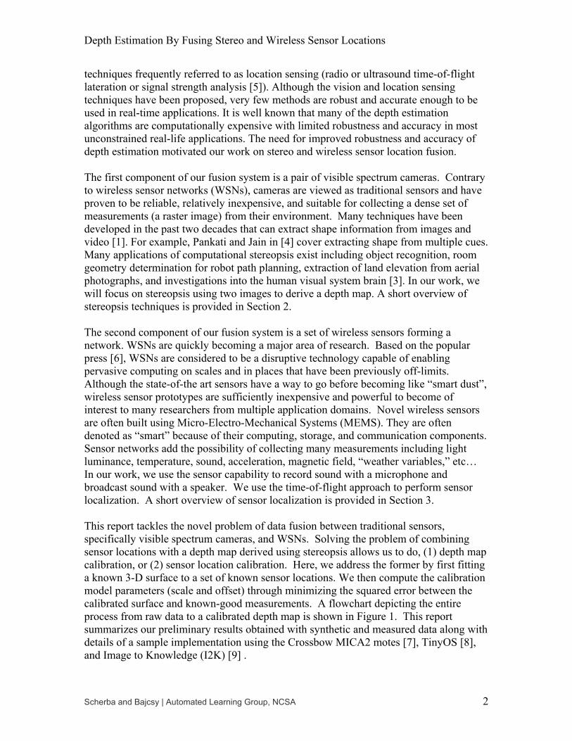
Stereopsis is the construction of three-dimensional geometry given multiple views of a scene as in [10], [11], [12]. Computational stereopsis is the science of using computers to perform stereopsis. Figure 2 shows a generalized stereopsis configuration. The cone on the checkerboard pattern represents a scene. Points C1, C2, and C3 represent optical centers of three [pinhole] cameras. I1, I2, and I3 represent the image planes of these cameras: the inputs to a stereopsis algorithm. In the general case, the stereopsis problem can be posed as the reconstruction of the scene geometry given the two-dimensional data (images) I1, I2, I3, …, In.

Figure 2: Generalized Stereopsis Configuration from [10].

2.2 Stereopsis with Two Images

A simplification of the general stereopsis configuration is the case with two images at a time (i.e. the number of input images n defined in section 2.1 is 2). As it is readily apparent from Figure 2, the 3-D reconstruction of a scene point is straight forward given matching points on the images. The scene point can be calculated as the intersection of



the two lines passing through the matched points and the optical centers. With known camera parameters, this setup reduces computational stereopsis to a problem of image matching. Some stereo image matching techniques are described in more detail in section 2.4. A natural question to ask is: “What can be determined if camera parameters are unknown?” The reference to camera parameters includes both intrinsic (e.g., lens distortions) and extrinsic (e.g., camera position) parameters. The intrinsic parameters are usually estimated from specification sheets provided by camera manufactures while the extrinsic parameters are controlled during the image acquisition, for example, by using stereo-rigs [11]. In this report, we do not consider the case of unknown intrinsic parameters and we deal with the case of unknown extrinsic parameters only. Unknown extrinsic parameters naturally occur when using images taken from unknown scene positions. Not having to rely on “stereo rigs” or precisely placed cameras is important in the “real world” as existing cameras are not likely to be of this type or need to be mobile (e.g. security cameras). It is well known that without extrinsic parameters, stereopsis can still extract 3-D geometry, albeit not to scale [12].

2.3 Stereo Rectification

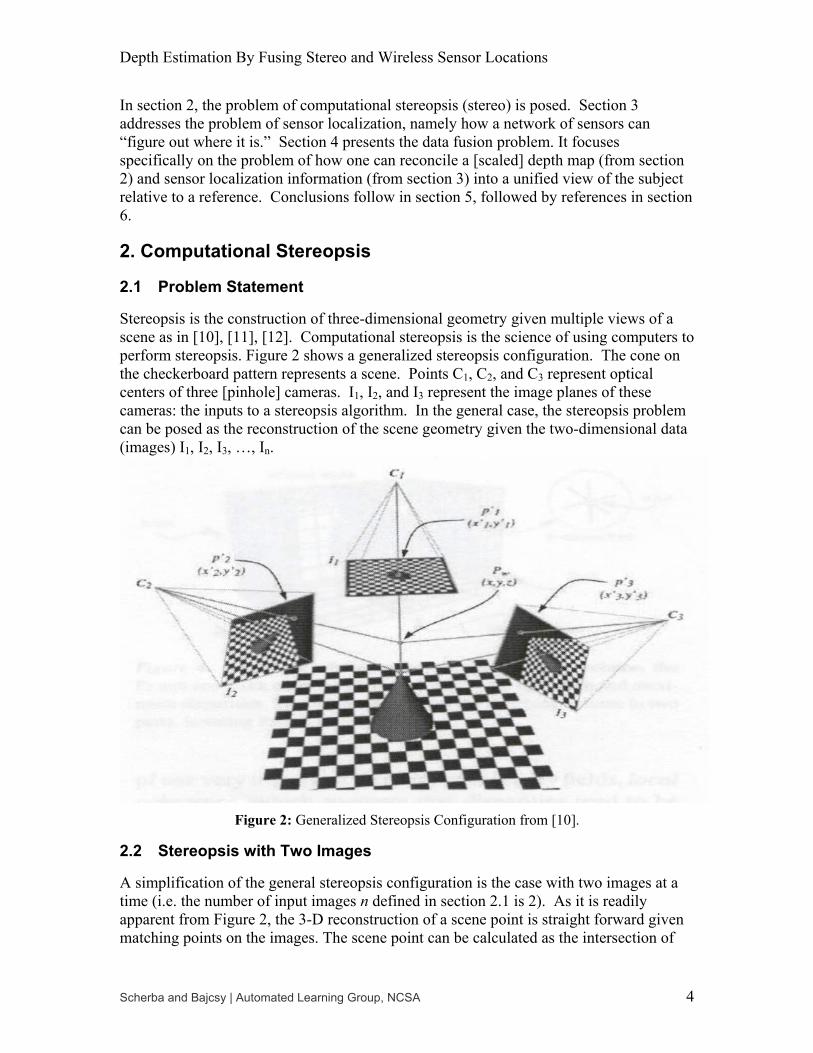
In this section, we focus on the special case of stereopsis without knowledge of extrinsic camera parameters. In this case, it is useful to perform “stereo rectification” on the images prior to attempting image matching. Stereo rectification is a process which aligns one of the images (taken to be the right image of a stereo pair in this report) such that matching points in the resulting images are on the same “scanline” (row or y-coordinate). The resulting images form a “rectified stereo pair” that corresponds to a configuration with cameras displaced purely horizontally from each other (see Figure 3).

Figure 3: Stereo Rectification

Stereo rectification serves two main purposes. First, it simplifies the geometry of the stereopsis problem tremendously. In the rectified images, everything can be expressed in terms of “disparity,” namely the distance between pixels in one image and the matching pixels in the other image (Figure 4). In general, each image point may have a unique disparity associated with it which is inversely proportional to the depth of that image

Rectified Image Plane

Rectified Image Plane

Actual Image Plane Actual Image

Plane



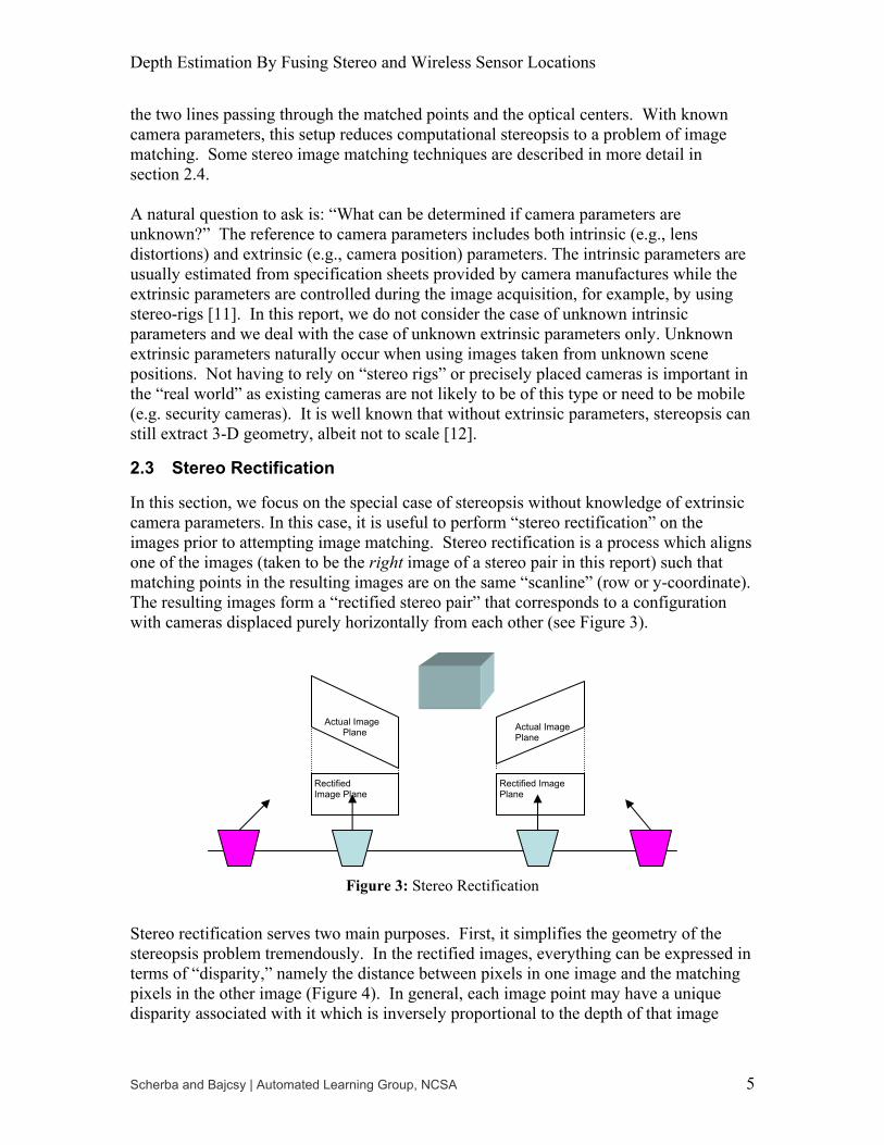
point in the scene. The second, and perhaps more important, purpose of stereo rectification is that the image matching task is simplified by using rectified images. If the rectification is successful, then the correct match for any pixel in an image would be found along the same scanline in the other image, and hence reduce a two-dimensional search per pixel to a one-dimensional search. This would only be useful if the rectification procedure is computationally faster than the difference between image matching using a two dimensional search and image matching using one dimensional search. We believe this to be the case.

Figure 4: Definition of Disparity

We decided to follow the approach proposed by Hartley in [13] and implement the algorithm as one of the Image To Knowledge (I2K) software tools [9]. Hartley’s technique allows us to find a “matched pair” of rectifying homographies (perspective projections), such that the epipole of the right image is mapped to infinity and epipolar lines in both images are equal. Isgro and Trucco describe an implementation of Hartley’s approach in [14]. Instead of finding and mapping the epipole manually (as Hartley suggests), Isgro and Trucco recognize that the fundamental matrix from a rectified pair of images is:

−=010100

000F

They then propose using pairs of matched image points to numerically compute the homographies using the Levenberg-Marquardt [15], [16] and standard linear least-squares algorithms. The former is used to minimize the following cost function:

( )[ ]∑=

=N

ii

ti pFHpHHHF

1

2

112221 ),(

The latter is used to minimize:

( ) ( )[ ]∑=

−N

ixixi pHpH

1

22211

d d'

'disparity dd −=



Minimizing this equation ensures that the rectified x-coordinates of the images are not displaced “too much” (i.e. that the image will not be ripped apart by the first constraint). Any pair of homographies satisfying these equations is sufficient, but we choose a pair of homographies so that H2 is constrained to be a rigid transformation about a point in space. To rectify an image pair, we just reproject the second (“right”) image using:

221

12 pHHp −=′ We have implemented this approach in the Image to Knowledge StereoRectify tool accessible through the Stereo Tool from the main menu (see the documentation on Stereo in [9]). Matching image points are currently specified by hand, as automatic image point/feature matching is another area of research beyond the scope of this report.

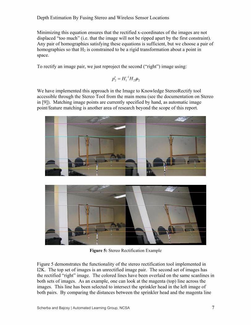
Figure 5: Stereo Rectification Example

Figure 5 demonstrates the functionality of the stereo rectification tool implemented in I2K. The top set of images is an unrectified image pair. The second set of images has the rectified “right” image. The colored lines have been overlaid on the same scanlines in both sets of images. As an example, one can look at the magenta (top) line across the images. This line has been selected to intersect the sprinkler head in the left image of both pairs. By comparing the distances between the sprinkler head and the magenta line



in the right images, one can obtain better understanding of what the stereo rectification algorithm accomplishes. A practical problem in the stereo rectification algorithm implementation is its sensitivity to the trivial solution of zero. The Levenberg-Marquardt numerical technique that is used is akin to a sophisticated gradient descent. A local minimum is desired, but the global minimum of zero is easily reached and has strong influence in practice. The rectified image displayed above, although improved in some ways, exhibits some behavior which can be attributed to this problem. Visibly, the column on the left side of the image is skewed in the rectified image more than one would expect for a simple, horizontal camera translation (the model that the rectified image pair should mirror). This, in turn, can mislead the image matching techniques discussed in section 2.4. Robust, automatic stereo rectification, although it would be useful, still appears to be a hard problem worthy of additional research. For the short-term, we decided on using image pairs which have already been rectified in order to mitigate the effects of stereo rectification problems.

2.4 Traditional Approaches to Stereo Matching

There are two predominant approaches to the stereo matching problem: correlation, and graph cuts. In both cases, the main obstacles to successful stereo matching are scene occlusions and mismatches. Correlation matching is simple in theory and can be described as follows. For each pixel in the left image, find a matching pixel along the same scanline in the right image by comparing two windows centered on the selected pixels using a correlation metric [17] . This scheme can be modified by (a) using adaptive windows, further limiting the search space along the scanline, or (b) doing the search in a multiscale fashion [18]. These modifications generally aim to increase the speed or robustness of the match. See section 2.5 for details on the modifications implemented to the correlation algorithm used in I2K. The main disadvantage of correlation matching is that every pixel fends for itself. This generally leads to good matches along each scanline, but can lead to inter-scanline discrepancies and errors (e.g. jagged edges of objects). Graph cut matching is similar to correlation matching in that a similar distance metric is used to decide what a good match is. Unlike correlation matching, graph cut techniques look to minimize global “costs” and can therefore penalize inter-scanline discrepancies. Briefly, graph cut methods formulate the stereo matching problem as a graph theoretic maximum flow problem. Solving the flow problem (using a known algorithm such as Edmunds-Karp [19]) also gives a depth map solution that minimizes a global cost given a penalty weight. The advantage to graph cut techniques is that they have produced one of the best computational stereopsis results to date [20]. The disadvantage of graph cut algorithms is their computational complexity: they are time-consuming relative to correlation (e.g. an execution can take many minutes for a single stereo pair). The problem of occlusions arises from regions of the stereo pair that are absent from either image. The algorithm for stereo matching cannot a priori determine occluding regions, so matching errors are highly likely in these regions. There has been



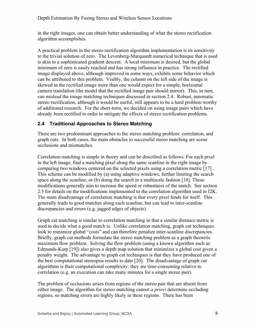
considerable research towards identifying and handling occluding regions [17], but these discussions are beyond the scope of this report. A simple strategy to detecting any occluding regions is to run stereo matching twice, the first time searching for matches to the left image and the second time searching for matches to the right image. If the two runs agree on disparities, the result is kept. If the two runs disagree on disparities, the result is thrown out and considered to be in an occluding region. Stereo mismatches can also occur when the image matching is not a one-to-one problem. This is very likely to happen if the scene does not contain any visually salient features (it could be called a visually “boring” scene), namely scenes which have wide areas with absolutely no details to match against (e.g. a white wall with even lighting), or scenes with man-made objects exhibiting regular patterns (e.g. textured areas, or similar features like the windows on a skyscraper in Figure 6). In all of the preceding cases, a small distance between [image matching] windows can mistakenly be classified as an incorrect match. A large number of incorrect matches will generally produce useless output. Using techniques discussed above to reduce the search space can help eliminate the effects of “boring” scenes. Similarly, global techniques, such as stereo using graph cuts, will avoid these problems. Global techniques would converge on a global minimum to promote the correct matches if given enough context. Other than these techniques, there is little that can be done algorithmically. One technique that does work in practice is to introduce texture into a scene (e.g. with large amounts of newspaper, or similar non-regular textures). We have used this method in some of our experiments with favorable results.

Figure 6: A hard-to-match object due to repetitive similar features (windows).

2.5 Stereo Matching in I2K

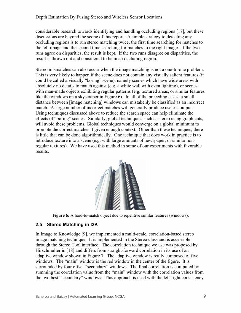
In Image to Knowledge [9], we implemented a multi-scale, correlation-based stereo image matching technique. It is implemented in the Stereo class and is accessible through the Stereo Tool interface. The correlation technique we use was proposed by Hirschmuller in [18] and differs from straight-forward correlation in its use of an adaptive window shown in Figure 7. The adaptive window is really composed of five windows. The “main” window is the red window in the center of the figure. It is surrounded by four offset “secondary” windows. The final correlation is computed by summing the correlation value from the “main” window with the correlation values from the two best “secondary” windows. This approach is used with the left-right consistency



check described in section 2.4 to identify occluded regions. All together, this algorithm corresponds with steps 1 through 4 of Hirschmuller’s algorithm in [18]. As shown in [18] and [20], this algorithm performs fairly well when compared with other stereo algorithms, especially those based on correlation, on reference stereo pairs. This algorithm is also termed as “real-time” in [18] and [20], although it is not in our implementation. The graph-cut algorithms, while producing higher quality results, are much harder to implement and have long running times. We did not use them in this report because of these reasons.

Figure 7: Adaptive Correlation Window

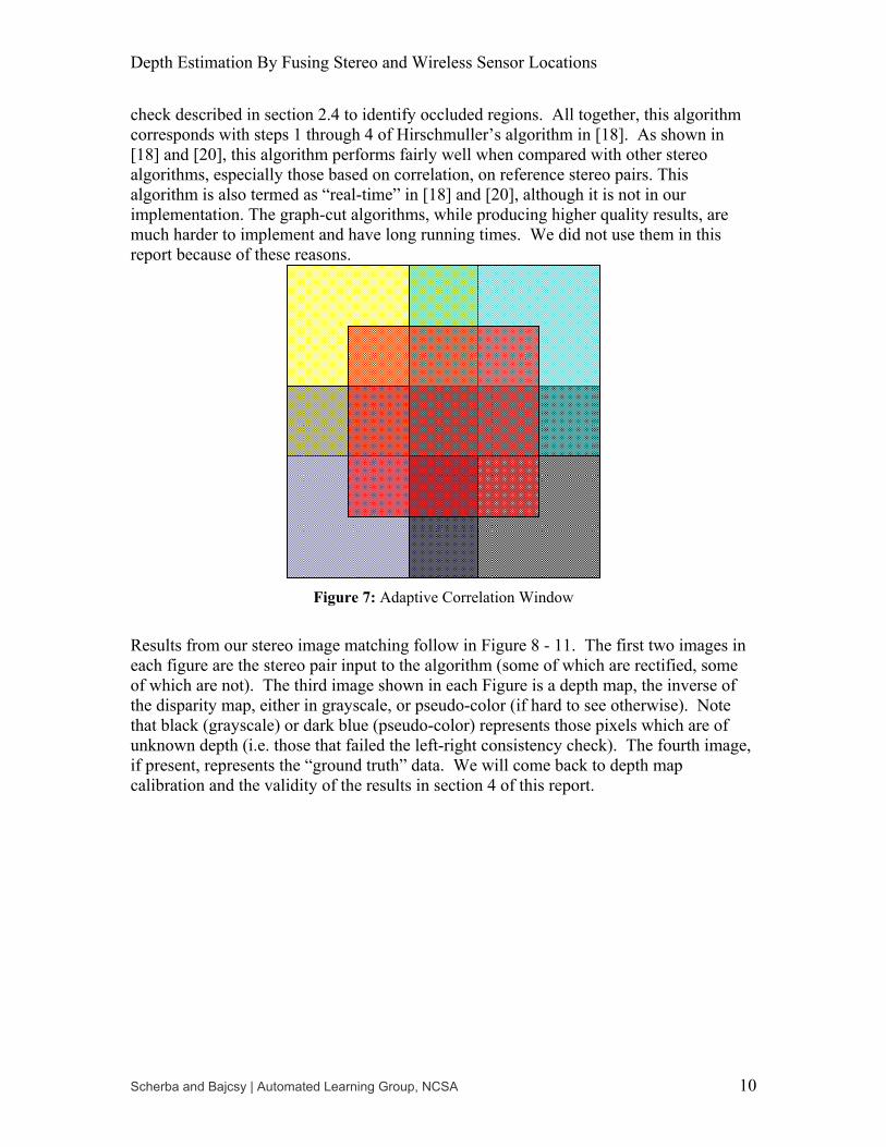
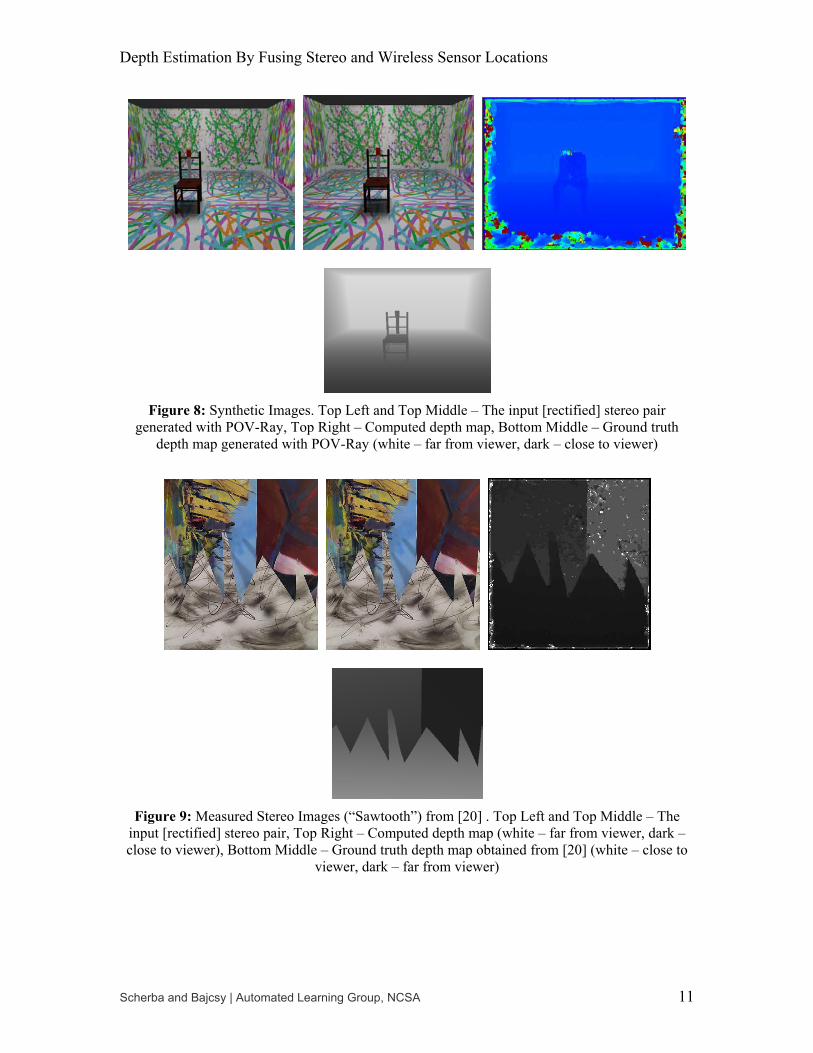
Results from our stereo image matching follow in Figure 8 - 11. The first two images in each figure are the stereo pair input to the algorithm (some of which are rectified, some of which are not). The third image shown in each Figure is a depth map, the inverse of the disparity map, either in grayscale, or pseudo-color (if hard to see otherwise). Note that black (grayscale) or dark blue (pseudo-color) represents those pixels which are of unknown depth (i.e. those that failed the left-right consistency check). The fourth image, if present, represents the “ground truth” data. We will come back to depth map calibration and the validity of the results in section 4 of this report.



Figure 8: Synthetic Images. Top Left and Top Middle – The input [rectified] stereo pair

generated with POV-Ray, Top Right – Computed depth map, Bottom Middle – Ground truth depth map generated with POV-Ray (white – far from viewer, dark – close to viewer)

Figure 9: Measured Stereo Images (“Sawtooth”) from [20] . Top Left and Top Middle – The

input [rectified] stereo pair, Top Right – Computed depth map (white – far from viewer, dark – close to viewer), Bottom Middle – Ground truth depth map obtained from [20] (white – close to

viewer, dark – far from viewer)



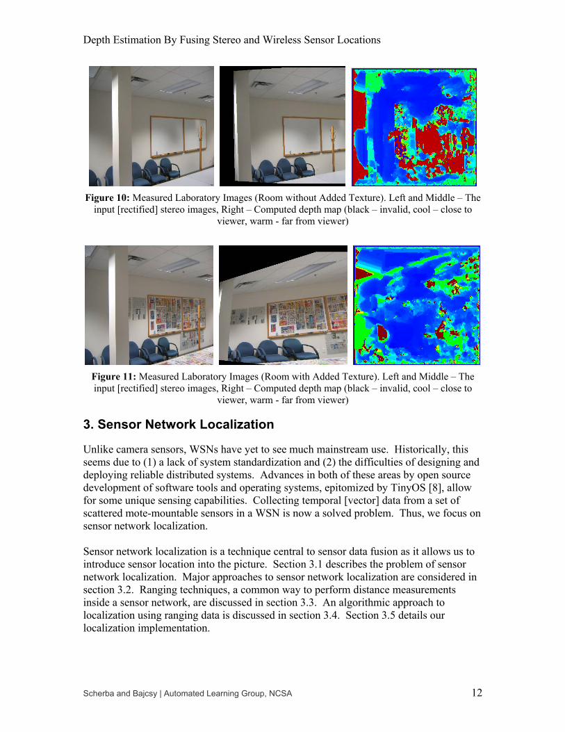
Figure 10: Measured Laboratory Images (Room without Added Texture). Left and Middle – The

input [rectified] stereo images, Right – Computed depth map (black – invalid, cool – close to viewer, warm - far from viewer)

Figure 11: Measured Laboratory Images (Room with Added Texture). Left and Middle – The input [rectified] stereo images, Right – Computed depth map (black – invalid, cool – close to

viewer, warm - far from viewer)

3. Sensor Network Localization

Unlike camera sensors, WSNs have yet to see much mainstream use. Historically, this seems due to (1) a lack of system standardization and (2) the difficulties of designing and deploying reliable distributed systems. Advances in both of these areas by open source development of software tools and operating systems, epitomized by TinyOS [8], allow for some unique sensing capabilities. Collecting temporal [vector] data from a set of scattered mote-mountable sensors in a WSN is now a solved problem. Thus, we focus on sensor network localization. Sensor network localization is a technique central to sensor data fusion as it allows us to introduce sensor location into the picture. Section 3.1 describes the problem of sensor network localization. Major approaches to sensor network localization are considered in section 3.2. Ranging techniques, a common way to perform distance measurements inside a sensor network, are discussed in section 3.3. An algorithmic approach to localization using ranging data is discussed in section 3.4. Section 3.5 details our localization implementation.




Sensor network localization is the problem of finding out the locations of all sensors in the network. Depending on the application, the localization problem can take many forms. For instance, in MIT’s Cricket application [21] localization is used to identify the room (or part of a room) that some sensor is in. This can be used for (a) service discovery, (b) enabling functionality (e.g. environmental control), or (c) providing functionality based on the high-level location of the device. For the applications we consider in this report, we are interested in knowing the coordinates of the sensors in space relative to a coordinate system defined by the position of one of our stereo cameras. In our implementation, the global coordinate system is centered on the left stereo camera.

3.2 Approaches to Sensor Network Localization

There are two major approaches to sensor network localization. The first approach relies on existing localization infrastructure, such as GPS. In this scenario, each mote in the network carries a GPS receiver [22]. The mote’s GPS receiver receives satellite broadcasts in order to find its global coordinates (i.e. latitude and longitude). The motes then convert these global coordinates into local coordinates relative to a chosen coordinate system. The major advantage of this localization system is that it is based on very solid technology. Current consumer GPS receivers [23] can provide an accurate measurement to within 5m using differential GPS techniques. The cons of this approach are cost, power consumption, fine-grained accuracy and areas not covered by GPS. The cost primary derives from the GPS receiver and antenna. These costs will presumably drop over time, but not relative to the cost of MEMS sensors. The power consumption comes from the radio (and currently an additional processor) that is needed to receive the GPS signal. Since a GPS receiver needs to be active (powered) for a bit while locating and tracking satellites, this is not a battery-friendly operation. There are many areas that do not receive a GPS signal, notably almost any indoor location. Finally, 5m accuracy may be fine on a global-level, but is not very useful on a laboratory-scale. Other localization techniques that rely on infrastructure exist (e.g. triangulation from cell phone towers, beacons similar to those used in MIT’s Cricket, etc…) and have similar tradeoffs. The second approach to sensor network localization does not rely on external infrastructure. Instead, motes in the network attempt to locate themselves relative to neighboring motes. This “relative localization” can be done in a number of ways. One straight-forward way is ranging, namely using a technique to find the Euclidean distance between two motes. In this report, we focus on the relative localization approach.

3.3 Ranging

3.3.1 Ranging Techniques

There are a number of ways to perform ranging as it is summarized in [5]. The most common [active] techniques are direct measurement, phase-based techniques, and techniques based on time of flight (ToF). Direct measurements are useful in static sensor



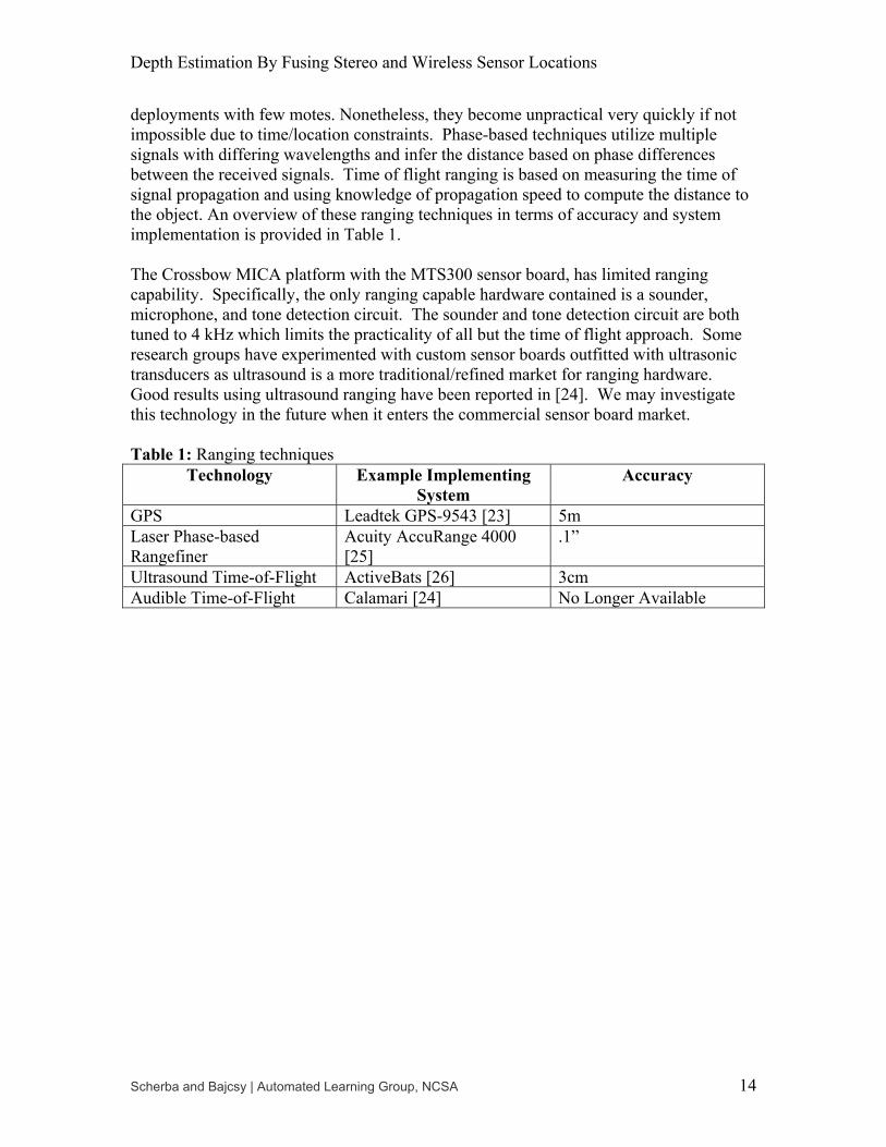
deployments with few motes. Nonetheless, they become unpractical very quickly if not impossible due to time/location constraints. Phase-based techniques utilize multiple signals with differing wavelengths and infer the distance based on phase differences between the received signals. Time of flight ranging is based on measuring the time of signal propagation and using knowledge of propagation speed to compute the distance to the object. An overview of these ranging techniques in terms of accuracy and system implementation is provided in Table 1. The Crossbow MICA platform with the MTS300 sensor board, has limited ranging capability. Specifically, the only ranging capable hardware contained is a sounder, microphone, and tone detection circuit. The sounder and tone detection circuit are both tuned to 4 kHz which limits the practicality of all but the time of flight approach. Some research groups have experimented with custom sensor boards outfitted with ultrasonic transducers as ultrasound is a more traditional/refined market for ranging hardware. Good results using ultrasound ranging have been reported in [24]. We may investigate this technology in the future when it enters the commercial sensor board market. Table 1: Ranging techniques

Technology Example Implementing System

Accuracy

GPS Leadtek GPS-9543 [23] 5m Laser Phase-based Rangefiner

Acuity AccuRange 4000 [25]

.1”

Ultrasound Time-of-Flight ActiveBats [26] 3cm Audible Time-of-Flight Calamari [24] No Longer Available



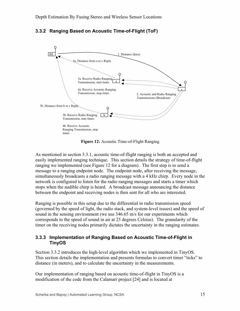
3.3.2 Ranging Based on Acoustic Time-of-Flight (ToF)

Figure 12: Acoustic Time-of-Flight Ranging

As mentioned in section 3.3.1, acoustic time-of-flight ranging is both an accepted and easily implemented ranging technique. This section details the strategy of time-of-flight ranging we implemented (see Figure 12 for a diagram). The first step is to send a message to a ranging endpoint node. The endpoint node, after receiving the message, simultaneously broadcasts a radio ranging message with a 4 kHz chirp. Every node in the network is configured to listen for the radio ranging messages and starts a timer which stops when the audible chirp is heard. A broadcast message announcing the distance between the endpoint and receiving nodes is then sent for all who are interested. Ranging is possible in this setup due to the differential in radio transmission speed (governed by the speed of light, the radio stack, and system-level issues) and the speed of sound in the sensing environment (we use 346.65 m/s for our experiments which corresponds to the speed of sound in air at 25 degrees Celsius). The granularity of the timer on the receiving nodes primarily dictates the uncertainty in the ranging estimates.

3.3.3 Implementation of Ranging Based on Acoustic Time-of-Flight in TinyOS

Section 3.3.2 introduces the high-level algorithm which we implemented in TinyOS. This section details the implementation and presents formulas to convert timer “ticks” to distance (in meters), and to calculate the uncertainty in the measurements. Our implementation of ranging based on acoustic time-of-flight in TinyOS is a modification of the code from the Calamari project [24] and is located at

1. Distance Query

3b. Receive Radio Ranging Transmission, start timer. 4b. Receive Acoustic Ranging Transmission, stop timer.

BS

3a. Receive Radio Ranging Transmission, start timer. 4a. Receive Acoustic Ranging Transmission, stop timer.

2. Acoustic and Radio Ranging Transmissions (Broadcast)

5a. Distance from a to c Reply

5b. Distance from b to c Reply

a

b

c



projects/ncsa/d2k/modules/projects/dscherba/tinyos-1.x/contrib/calamari. The released Calamari code was designed for ultrasonic sensors using the MICA platform, not the MICA2. We modified the code to use the piezo-electric buzzer, microphone, and tone-detection circuit present on the MTS300 (basicsb) sensor board. We kept the timer granularity at the default 1/1024s (approximately 1 millisecond).

3.4 Algorithmic Approaches

As mentioned in section 3.1, the goal of localization is to find coordinates of sensors in a given coordinate system. This section addresses the problem of converting ranging data, as collected by techniques discussed in section 3.3, into localization information. This problem is not always solvable, but the pathologic cases tend not to appear in practice [27]. The authors of the technical report [27] frame the problem in a graph theoretic manner. Let each mote be a node, and let the average ranging distance between motes be the undirected edge lengths. If a three dimensional embedding of the above graph exists and is globally rigid, we have a valid solution to the localization problem. The approach suggested in [27] to find such a solution has two steps: first the graph is “unfolded,” then an iterative, mass and spring graph relaxation technique is used. The “resting lengths” of the springs are the ranging distances, so the solution will even handle errors in ranging by converging to a “minimum energy” configuration.

3.5 Localization Results

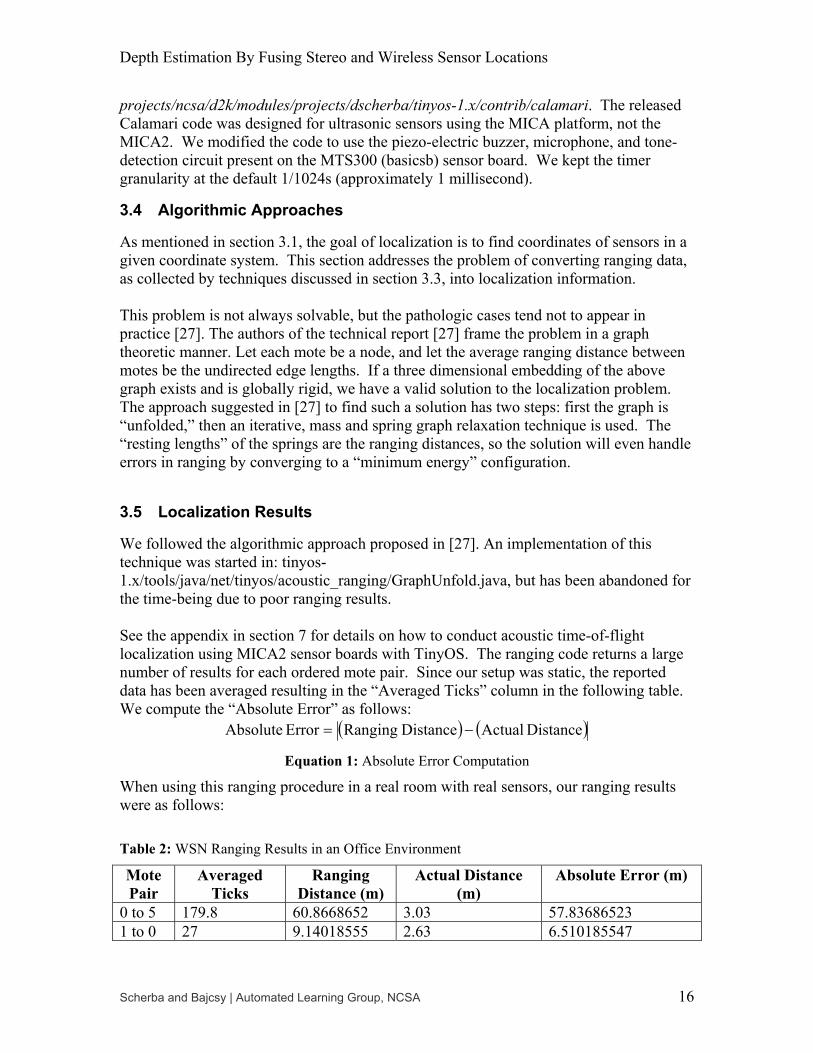
We followed the algorithmic approach proposed in [27]. An implementation of this technique was started in: tinyos-1.x/tools/java/net/tinyos/acoustic_ranging/GraphUnfold.java, but has been abandoned for the time-being due to poor ranging results. See the appendix in section 7 for details on how to conduct acoustic time-of-flight localization using MICA2 sensor boards with TinyOS. The ranging code returns a large number of results for each ordered mote pair. Since our setup was static, the reported data has been averaged resulting in the “Averaged Ticks” column in the following table. We compute the “Absolute Error” as follows:

( ) ( )Distance ActualDistance RangingError Absolute −=

Equation 1: Absolute Error Computation

When using this ranging procedure in a real room with real sensors, our ranging results were as follows: Table 2: WSN Ranging Results in an Office Environment

Mote Pair

Averaged Ticks

Ranging Distance (m)

Actual Distance (m)

Absolute Error (m)

0 to 5 179.8 60.8668652 3.03 57.83686523 1 to 0 27 9.14018555 2.63 6.510185547



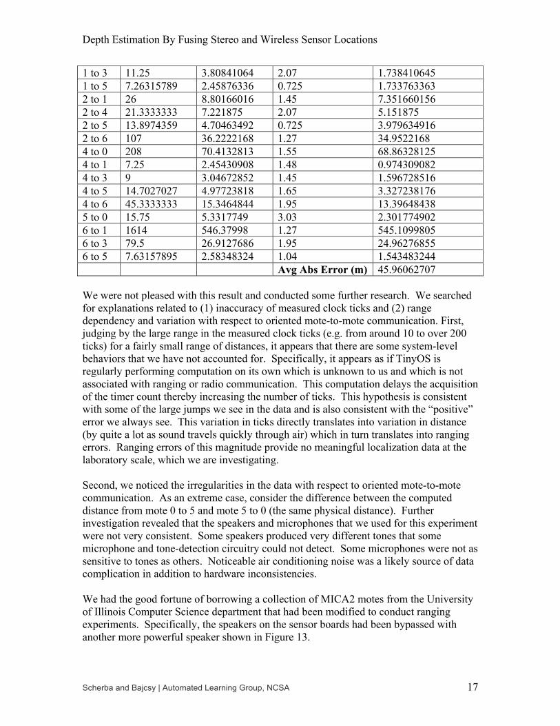
1 to 3 11.25 3.80841064 2.07 1.738410645 1 to 5 7.26315789 2.45876336 0.725 1.733763363 2 to 1 26 8.80166016 1.45 7.351660156 2 to 4 21.3333333 7.221875 2.07 5.151875 2 to 5 13.8974359 4.70463492 0.725 3.979634916 2 to 6 107 36.2222168 1.27 34.9522168 4 to 0 208 70.4132813 1.55 68.86328125 4 to 1 7.25 2.45430908 1.48 0.974309082 4 to 3 9 3.04672852 1.45 1.596728516 4 to 5 14.7027027 4.97723818 1.65 3.327238176 4 to 6 45.3333333 15.3464844 1.95 13.39648438 5 to 0 15.75 5.3317749 3.03 2.301774902 6 to 1 1614 546.37998 1.27 545.1099805 6 to 3 79.5 26.9127686 1.95 24.96276855 6 to 5 7.63157895 2.58348324 1.04 1.543483244 Avg Abs Error (m) 45.96062707 We were not pleased with this result and conducted some further research. We searched for explanations related to (1) inaccuracy of measured clock ticks and (2) range dependency and variation with respect to oriented mote-to-mote communication. First, judging by the large range in the measured clock ticks (e.g. from around 10 to over 200 ticks) for a fairly small range of distances, it appears that there are some system-level behaviors that we have not accounted for. Specifically, it appears as if TinyOS is regularly performing computation on its own which is unknown to us and which is not associated with ranging or radio communication. This computation delays the acquisition of the timer count thereby increasing the number of ticks. This hypothesis is consistent with some of the large jumps we see in the data and is also consistent with the “positive” error we always see. This variation in ticks directly translates into variation in distance (by quite a lot as sound travels quickly through air) which in turn translates into ranging errors. Ranging errors of this magnitude provide no meaningful localization data at the laboratory scale, which we are investigating. Second, we noticed the irregularities in the data with respect to oriented mote-to-mote communication. As an extreme case, consider the difference between the computed distance from mote 0 to 5 and mote 5 to 0 (the same physical distance). Further investigation revealed that the speakers and microphones that we used for this experiment were not very consistent. Some speakers produced very different tones that some microphone and tone-detection circuitry could not detect. Some microphones were not as sensitive to tones as others. Noticeable air conditioning noise was a likely source of data complication in addition to hardware inconsistencies. We had the good fortune of borrowing a collection of MICA2 motes from the University of Illinois Computer Science department that had been modified to conduct ranging experiments. Specifically, the speakers on the sensor boards had been bypassed with another more powerful speaker shown in Figure 13.



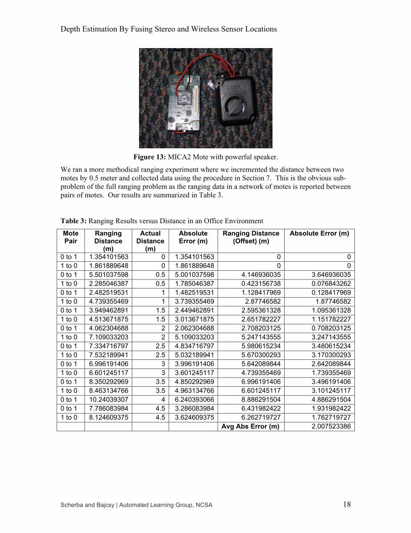
Figure 13: MICA2 Mote with powerful speaker.

We ran a more methodical ranging experiment where we incremented the distance between two motes by 0.5 meter and collected data using the procedure in Section 7. This is the obvious sub-problem of the full ranging problem as the ranging data in a network of motes is reported between pairs of motes. Our results are summarized in Table 3.

Table 3: Ranging Results versus Distance in an Office Environment

Mote Pair

Ranging Distance

(m)

Actual Distance

(m)

Absolute Error (m)

Ranging Distance (Offset) (m)

Absolute Error (m)

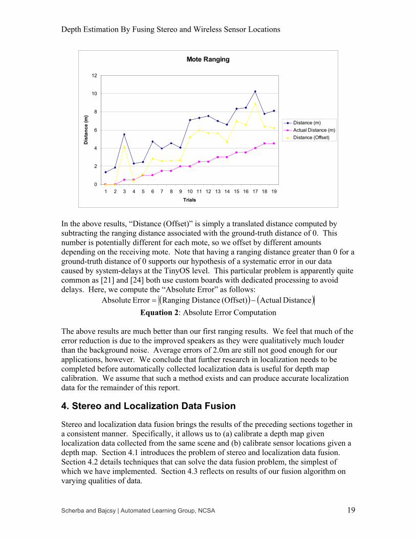
0 to 1 1.354101563 0 1.354101563 0 01 to 0 1.861889648 0 1.861889648 0 00 to 1 5.501037598 0.5 5.001037598 4.146936035 3.6469360351 to 0 2.285046387 0.5 1.785046387 0.423156738 0.0768432620 to 1 2.482519531 1 1.482519531 1.128417969 0.1284179691 to 0 4.739355469 1 3.739355469 2.87746582 1.877465820 to 1 3.949462891 1.5 2.449462891 2.595361328 1.0953613281 to 0 4.513671875 1.5 3.013671875 2.651782227 1.1517822270 to 1 4.062304688 2 2.062304688 2.708203125 0.7082031251 to 0 7.109033203 2 5.109033203 5.247143555 3.2471435550 to 1 7.334716797 2.5 4.834716797 5.980615234 3.4806152341 to 0 7.532189941 2.5 5.032189941 5.670300293 3.1703002930 to 1 6.996191406 3 3.996191406 5.642089844 2.6420898441 to 0 6.601245117 3 3.601245117 4.739355469 1.7393554690 to 1 8.350292969 3.5 4.850292969 6.996191406 3.4961914061 to 0 8.463134766 3.5 4.963134766 6.601245117 3.1012451170 to 1 10.24039307 4 6.240393066 8.886291504 4.8862915040 to 1 7.786083984 4.5 3.286083984 6.431982422 1.9319824221 to 0 8.124609375 4.5 3.624609375 6.262719727 1.762719727 Avg Abs Error (m) 2.007523386



Mote Ranging

0

2

4

6

8

10

12

1 2 3 4 5 6 7 8 9 10 11 12 13 14 15 16 17 18 19

Trials

Dis

tanc

e (m

)

Distance (m)Actual Distance (m)Distance (Offset)

In the above results, “Distance (Offset)” is simply a translated distance computed by subtracting the ranging distance associated with the ground-truth distance of 0. This number is potentially different for each mote, so we offset by different amounts depending on the receiving mote. Note that having a ranging distance greater than 0 for a ground-truth distance of 0 supports our hypothesis of a systematic error in our data caused by system-delays at the TinyOS level. This particular problem is apparently quite common as [21] and [24] both use custom boards with dedicated processing to avoid delays. Here, we compute the “Absolute Error” as follows:

( ) ( )Distance Actual(Offset) Distance RangingError Absolute −= Equation 2: Absolute Error Computation

The above results are much better than our first ranging results. We feel that much of the error reduction is due to the improved speakers as they were qualitatively much louder than the background noise. Average errors of 2.0m are still not good enough for our applications, however. We conclude that further research in localization needs to be completed before automatically collected localization data is useful for depth map calibration. We assume that such a method exists and can produce accurate localization data for the remainder of this report.

4. Stereo and Localization Data Fusion

Stereo and localization data fusion brings the results of the preceding sections together in a consistent manner. Specifically, it allows us to (a) calibrate a depth map given localization data collected from the same scene and (b) calibrate sensor locations given a depth map. Section 4.1 introduces the problem of stereo and localization data fusion. Section 4.2 details techniques that can solve the data fusion problem, the simplest of which we have implemented. Section 4.3 reflects on results of our fusion algorithm on varying qualities of data.




In this report, we formulate the stereo and localization data fusion problem as the problem of calibrating the depth map (obtained through computational stereopsis) using the localization data (obtained from the wireless sensor network). Theoretically, the depth map is correct up to a scaling factor, so the problem reduces to the problem of calculating the scaling factor. We look at solving the [more general] problem of a scaling factor and an offset. The offset can presumably handle some systematic errors that we have unknowingly introduced by our techniques. In summary, Equation 3 defines the depth map calibration relation.

βα += mapdepth zz calibmapdepth

Equation 3: Depth Map Calibration Relation

4.2 Proposed Approach

The primary challenge in the data fusion problem is the registration of the depth map image with the wireless sensor locations. We are looking for depth map image locations where a sensor lies. This could be viewed as a matching problem assuming that a sensor shape or its intensity profile is uniquely defined with respect to all other scene objects. We have considered two approaches to this registration problem.

In the first approach, a user manually specifies the correspondences (as we have done above for the stereo rectification problem). This consists of manually identifying pixels in the depth map (or the corresponding left stereo image) of a known sensor ID. If the localization step is completed successfully, knowing the sensor ID is equivalent to knowing the depth coordinate of the sensor, calib

mapdepthzz =sensor .

In the second approach, one can place sensors on visible planar surfaces in a sufficiently dense fashion. By incorporating the spatial arrangement of sensors, we can automate parts of the calibration as described in the following procedure. The sensor locations in a depth map image coordinate system are manually selected, and the calibration program fits the sensor locations to a plane in the 3-D “world” coordinate system. This plane is used for depth map calibration since in the “camera” coordinate system, the image points corresponding to the sensors will also form a plane. The depth map calibration is based on the fact that all sensor locations relative to an arbitrary point taken to be the “left” camera, in our setup, are known to be within scale, offset, and rotational factors (i.e. five degrees of freedom). In this work, we use the second approach for fusing stereo and wireless sensor locations. In general, one would desire to identify a large plane, both in terms of sensors falling on it, and in percentage of image covered. Techniques for finding a planar subset in a collection of 3-D points exist in the literature, for instance in [28]. We avoided this problem by manually selecting points from the stereo pair that lie on a plane in a world coordinate system defined by the left camera.



We continue by finding the parameters of the plane in 3-D that fits the sensor ”world” coordinate locations using a linear least squares approach and minimizing the squared error in z (the axis perpendicular to the image plane). We fit the plane

0=+−+ dzbyax to the sensor real-world coordinate locations. Using the computed plane parameters (a, b, d) we then make the substitution for calib

mapdepthz using Equation 3 and solve (in a linear least squares fashion) the resulting problem over all known points to obtain α and β. At this point the depth map can be calibrated and the results compared against what is known.

4.3 Experimental Results

Section 4.2 covered the implementation of the fusion algorithm used in Image to Knowledge. Section 4.3.1 covers the details of our evaluation methodology for this algorithm. The quantitative results from our experiments are reported in section 4.3.2.

4.3.1 Methodology for Accuracy Evaluations

Ultimately, we measure our fusion performance by the accuracy of the resulting depth map relative to a ground truth depth map. In practice, the ground truth depth map is generally not available, or is very difficult to obtain. The situation is a bit different in our experimental setup as we have the ability to acquire ground truth measurements. We conducted experiments with theoretical/synthesized stereo pairs and actual/measured stereo pairs. In the synthetic image case (e.g. Figure 8), we can generate a dense, theoretically correct depth map. In the real-world cases, we do not have the luxury of a dense depth map and must resort to a relatively small set of points at hand-verified distances. Another issue is the error metric for comparing ground truth depth maps with estimated depth maps. We consider two error metrics: (a) the average absolute distance error for each pixel/hand-verified point, and (b) the average absolute distance error as a percentage of maximum measured range in the image. Both values decrease with more accurate calibration (fusion) and are asymptotically optimal (zero). The accuracy evaluation methodology for each set of input images is outlined next.

4.3.1.1 Methodology for Synthetic Images

1. Create a synthetic stereo pair 2. Compute a theoretical depth map based on the geometry of the scene1 3. Compute an uncalibrated depth map mapdepthz from a stereo pair of images using

the I2K Stereo tool. 4. Using four points from step 2 that fall in a plane, calibrate the depth map from

step 3 using the I2K Stereo tool to obtain calibmapdepthz based on Equation 3

5. Compute the average absolute distance error using all image points (perhaps excluding a border of a given width)2

1 One way to do this if using a ray tracer like POVRay is by texturing the entire scene with an “ambient” colormap linearly changing from black to white and centered at the camera



6. Compute the average absolute distance percentage of maximum measured range. The maximum distance of the points from step 2 is “Max Range” and we use:

%100Range)(Max

Error) Dist. Abs. (Avg. RangeMax of %Error ⋅=

4.3.1.2 Methodology for Real Images 1. Take a stereo pair of a real scene 2. Record manually distance measurements to N points (N>4) in the scene. Four of

these points will be used for calibration and should lie in a plane. One point should represent the maximum range of the image (used in step 6)

3. Compute an uncalibrated depth map mapdepthz from a stereo pair of images using the I2K Stereo tool.

4. Using the four points from step 2, calibrate the depth map to obtain calibmapdepthz based

on Equation 3 5. Compute the average absolute distance error using all points from step 2:

∑∈

−=Points

)()(1Error Dist. Abs. Avg.i

actualcalib

mapdepth izizN

6. Compute the average absolute distance percentage of maximum measured range. The maximum distance of the points from step 2 is “Max Range” and we use:

%100Range)(Max

Error) Dist. Abs. (Avg. RangeMax of %Error ⋅=

4.3.2 Results

We performed a number of different experiments in order to evaluate quantitatively the accuracy of results as a function of scene texture and calibration model complexity. Specifically, we conducted experiments that change the amount of texture in the scene (which affects the quality of the stereo output). We also include results which have been calibrated using only “scaled” depth maps (assuming 0=β ). We observed that the calibration results under the assumption of 0=β led to smaller error in some cases, seemingly due to the sensitivity of calibration to the quality of the plane fit.

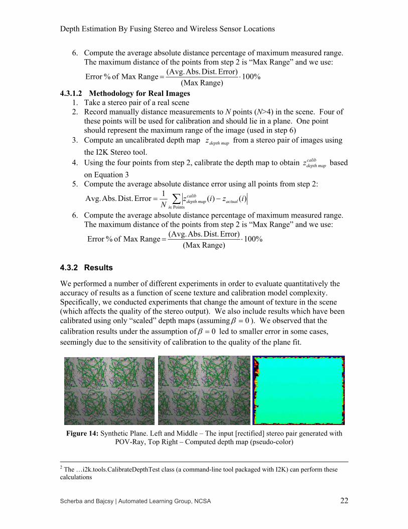
Figure 14: Synthetic Plane. Left and Middle – The input [rectified] stereo pair generated with

POV-Ray, Top Right – Computed depth map (pseudo-color)

2 The …i2k.tools.CalibrateDepthTest class (a command-line tool packaged with I2K) can perform these calculations



As an algorithm test, we generated a synthetic stereo pair (Figure 14) consisting of a single plane perpendicular to the camera (e.g. a normal pointing along the z-axis). We fitted a plane to four image points, as before, and verified that the fitted plane had a normal along the z-axis regardless of the specific implementation of a stereo method. The scale and offset factors differed, however, leading to differing errors in the calibrated depth map. Our results (excluding a border of width 100 pixels) are summarized in Table 4. Table 4: Results obtained for a synthetic stereo pair consisting of a single plane perpendicular to the camera. Number of

Points Scale α

Offset β

Avg. Absolute

Dist. Error

Maximum Image Range

Error % of Max Range

Scale Only

57408 .616 N/A 0.512 12 4.26%

Scale and Offset

57408 -.702 19.925 0.054 12 0.45%

During testing with real stereo pairs, the phenomenon of near-zero scaling factors occurred numerous times, creating very large calibration errors. We feel this arises due to overfitting of our calibration points. The errors in the chosen points allow for a local minimum “fit” that is just their average (i.e. purely an offset), rather than a purely scaled, or mixed solution that approaches the global minimum error. Theory predicts that scaling is the only operation needed to achieve the global minimum, so incorporating this a priori knowledge into the fitting step is the “correct” thing to do. In real and synthetic stereo pairs, this is not always true, possibly due to unknown systematic errors. Fortunately, both “scaling” and “scaling and offsetting” result in empirically similar numbers, suggesting that either choice will work. We present both figures in our calibration results:



Table 5: Calibration Evaluations

Stereo Pair Number of Points

Avg. Absolute

Dist. Error 0,0 ≠≠ βα

Avg. Absolute

Dist. Error (“scaled only” or

0=β )

Maximum Image Range

Error % of Max Range (Scale and

Offset/Scale)

Synthetic 17808 7.664 2.731 12 63.8% 22.76%

Untextured Room

15 1.771m 2.546m 7.7m 23% 33.1%

Textured Room

15 1.269m 1.412m 7.7m 16.5% 11.8%

Interestingly, we find that performance with measured images is better than performance with synthetic images in terms of distance accuracy as a percentage of maximum image range, a useful measure of calibration accuracy. We attribute this to the simplicity of our synthetic scene compared with the complexity of the actual room. In the actual room, especially in the textured case, there are more unique “textures” that the stereo algorithm can match against resulting in a better depth map. Similarly, performance is better in the textured room than in the untextured room for the same reason. Another reason for the difference between the synthetic and measured performance is due to the density of ground truth points. In the actual room, we measured only certain, “easily identifiable” points, while in the synthetic scene we knew 3-D locations of all image points. We do not have data on how these range estimates compare with range estimates obtained with calibrated cameras (i.e. when the intrinsic and extrinsic parameters of both cameras are known). We leave this comparison as an area for future research.

5. Conclusion

We presented the results of a preliminary study about depth estimation by fusing stereo and wireless sensor locations. Depth map calibration is one possible application of such fusion. For this application to become feasible, more research needs to be done on the underlying problems, especially on algorithms that do not require human intervention. On the infrastructural level, accurate ranging in wireless sensor networks remains a problem. Some of this may be alleviated with future commercial developments (and related software), such as ultrasound boards. On the algorithmic level, robust techniques for matching image points need to be explored. While this is a largely solved problem in the computational stereopsis domain, it remains a problem for those cases where image coordinates corresponding to sensors must be found. These points are critical in the calibration step, but have been manually specified in this report. Once these problems have been solved, this application may become very useful as it does not require the use of precise cameras or calibrated stereo rigs. As wireless sensor networks and pervasive



computing take off and become a commercial reality, this capability can be the underlying layer of high-level recognition and response mechanisms: one piece of a “smarter” world.



6. References

[1] H. Wechsler, Computational Vision, Boston: Academic Press, 1990.

[2] P. Dario, M. Bergamasco, A. Bicchi, and A. Fiorillo, “Multiple Sensing for Dexterous End Effectors,” Robots with Redundancy: Design, Sensing and Control, A.K. Bajcsy, ed., Berlin: Springer Verlag, 1992.

[3] D. Marr, Vision, San Francisco: W.H. Freeman, 1982.

[4] S. Pankanti and A.K. Jain, “Integrating Vision Modules: Stereo, Shading, Grouping, and Line Labeling,” PAMI, Vol. 17, Num. 9, Sep. 1995, pp 831-842.

[5] J. Hightower and G. Borriello, “Location Systems for Ubiquitous Computing,” IEEE Computer, Vol. 34, Num. 8, Aug. 2001, pp. 57-66.

[6] W. Roush, A.M. Goho, E. Scigliano, D. Talbot, M.M. Waldrop, G.T. Huang, P. Fairley, E. Jonietz, and H. Brody, “10 Emerging Technologies,” Technology Review, Vol. 106, No. 1, 2003, pp 33-46.

[7] Crossbow Technologies, Inc., “MPR400 MICA2 Datasheet,” Aug. 2004; http://www.xbow.com/Products/Product_pdf_files/Wireless_pdf/ 6020-0042-05_A_MICA2.pdf.

[8] UC Berkeley, “TinyOS Community Forum,” Aug. 2004; http://www.tinyos.net/.

[9] P. Bajcsy et. al. “I2K – Image to Knowledge,” Software documentation, ALG, NCSA, UIUC, Aug. 2004; http://alg.ncsa.uiuc.edu/do/tools/i2k/.

[10] S. Roy, “Stereo Without Epipolar Lines: A Maximum-Flow Formulation,” International Journal of Computer Vision, Vol 34, No. 2/3, 1999, pp 147-161.

[11] R. Sara, “Accurate Natural Surface Reconstruction from Polynocular Stereo” in Confluence of Computer Vision and Computer Graphics, Ed. A. Leonardis, et al, Boston: Kluwer Academic Publishers, 1999.

[12] U. Dhond and J.K. Aggarwal, "Structure from Stereo--A Review," IEEE Transactions of Systems, Man, and Cybernetics, Vol. 19, No. 6, Nov 1989, pp 1489-1510.

[13] R.I. Hartley, “Theory and Practice of Projective Rectification,” International Journal of Computer Vision, Vol. 35, No. 2, 1999, pp 115-127.

[14] F. Isgro and E. Trucco, “Projective Rectification without Epipolar Geometry,” Computer Vision and Pattern Recognition (CVPR), Vol. 1, June 1999, pp 94-99.

[15] W.H. Press, S.A. Teukolsky, W.T. Vetterling, and B.P. Flannery, Numerical Recipes in C: The Art of Scientific Computing, Cambridge University Press, 1992.



[16] J.P. Lewis, “LM.java (Levenberg-Marquardt),” Aug. 2004; http://www.idiom.com/~zilla/Computer/Javanumeric/LM.java.

[17] M.Z. Brown, D. Burschka and G.D. Hager, “Advances in Computational Stereo,” IEEE Transactions on Pattern Analysis and Machine Intelligence (PAMI), Vol. 25, No. 8, Aug. 2003, pp 993-1008.

[18] H. Hirschnuller, “Improvements in Real-Time Correlation-Based Stereo Vision,” IEEE Workshop on Stereo and Multi-Baseline Vision, Kauai, Hawaii, Dec. 2001, pp 141-148.

[19] T.H. Cormen, C.E. Leiserson, and R.L. Rivest, Introduction to Algorithms, The MIT Press, 1990.

[20] D. Scharstein and R. Szeliski, “Middlebury Stereo Vision Page,” Aug. 2004; http://cat.middlebury.edu/stereo/.

[21] Network and Mobile Systems Group, CSAIL, MIT, “The Cricket Indoor Location System,” Aug. 2004; http://nms.lcs.mit.edu/projects/cricket/.

[22] Crossbow Technologies, Inc., “MTS400/MTS420 DataSheet,” Aug. 2004; http://www.xbow.com/Products/Product_pdf_files/Wireless_pdf/ 6020-0053-01_B_MTS400-420.pdf.

[23] Leadtek Research, Inc., “GPS-9543 Datasheet,” Aug. 2004; http://www.leadtek.com/datasheet/gps-oem-module.pdf.

[24] K. Whitehouse and X. Jiang, “Calamari: A Localization System for Sensor Networks,” Aug. 2004; http://www.cs.berkeley.edu/~kamin/calamari/.

[25] Schmitt Measurement Systems, Inc., “Acuity AR4000 Datasheet,” Aug. 2004; http://www.acuityresearch.com/pdf/ar4000-data-sheet.pdf.

[26] AT&T Laboratories Cambridge, “The Bat Ultrasonic Location System,” Aug. 2004; http://www.uk.research.att.com/bat/.

[27] N.B. Priyantha, H. Balakrishnan, E. Demaine, and S. Teller, “Anchor-Free Distributed Localization in Sensor Networks,” Tech Report 892, Laboratory for Computer Science, MIT, 2003.

[28] K. Okada, S. Kagami, M. Inaba, and H. Inoue, “Plane Segment Finder: Algorithm, Implementation and Applications,” Proceedings IEEE International Conference on Robotics & Automation, Seoul, Korea, May. 2001, pp 2120 – 2125.

[29] M. Bergamasco, P. Dario, A. Bicchi, and G. Buttazzo, “Multi Sensor Integration for Fine Manipulation,” Highly Redundant Sensing in Robotic Systems, J.T. Tou, ed., J.G. Balchen, ed., NATO-ASI Series F: Computer and Systems Sciences, Berlin: Springer Verlag, Vol. 58, 1990, pp 55-66.



7. Appendix A: Acoustic Time-of-Flight Ranging

This appendix describes the procedure for conducting time-of-flight ranging using the modified Calamari code. A working knowledge of TinyOS and sensor hardware is assumed and can be gained through the material at [8]. The required hardware for acoustic time-of-flight ranging is fairly minimal:

• Base station (with mote) • PC with Java to connect with base station • MICA2 motes (one for each node including the origin) • “basicsb” sensor boards with microphones and sounders for each node

Programming the motes is also straight-forward. Note that the Active Message group (used in TinyOS communication) is 0xdd in the Calamari-derived code. 0x7d is the default group for TinyOS, so you will need to adjust the TOSBase build process to listen for this group. This can be done with the following addition to TOSBase/Makefile: DEFAULT_LOCAL_GROUP=0xdd The preceding addition should be made before any “include” lines to ensure that it will work. To program the motes, do the following (path names relative to the TinyOS root directory in the CVS code archive, namely projects/ncsa/d2k/modules/projects/dscherba/tinyos-1.x):

1. Program the base station with apps/TOSBase 2. Program all of the nodes with:

contrib/calamari/micaRangingApp/TransceiverApp.nc using unique numeric identifiers

At this point, the motes can be turned on and deployed. To start the ranging, run the tools.java.net.tinyos.acoustic_ranging.acoustic_ranging Java class. This code will dump its output (with the raw ranging results in ticks) into a file named “moteMap.out” in the current directory. This file is actually a serialized class that can be used as input to other analysis programs. With time we hope to make this interface more transparent and suitable for input into non-specialized tools (i.e. a text or XML file).

Depth Estimation by Fusing Stereo and Wireless Sensor Locations

Documents

Transcript of Depth Estimation by Fusing Stereo and Wireless Sensor Locations