Deposition fluxes of terpenes over grassland

I. Bamberger,1 L. Hörtnagl,2 T. M. Ruuskanen,1,3 R. Schnitzhofer,1,4 M. Müller,1

M. Graus,1,5,6 T. Karl,1,7 G. Wohlfahrt,2 and A. Hansel1

Received 9 December 2010; revised 23 May 2011; accepted 3 June 2011; published 27 July 2011.

[1] Eddy covariance flux measurements were carried out for two subsequentvegetation periods above a temperate mountain grassland in an alpine valley using aproton‐transfer‐reaction‐mass spectrometer (PTR‐MS) and a PTR time‐of‐flight‐massspectrometer (PTR‐TOF). In 2008 and during the first half of the vegetation period 2009the volume mixing ratios (VMRs) for the sum of monoterpenes (MTs) were typically wellbelow 1 ppbv and neither MT emission nor deposition was observed. After a hailstorm inJuly 2009 an order of magnitude higher amount of terpenes was transported to the sitefrom nearby coniferous forests causing elevated VMRs. As a consequence, depositionfluxes of terpenes to the grassland, which continued over a time period of several weekswithout significant reemission, were observed. For days without precipitation thedeposition occurred at velocities close to the aerodynamic limit. In addition tomonoterpene uptake, deposition fluxes of the sum of sesquiterpenes (SQTs) and the sum ofoxygenated terpenes (OTs) were detected. Considering an entire growing season for thegrassland (i.e., 1 April to 1 November 2009), the cumulative carbon deposition ofmonoterpenes reached 276 mg C m−2. This is comparable to the net carbon emissionof methanol (329 mg C m−2), which is the dominant nonmethane volatile organiccompound (VOC) emitted from this site, during the same time period. It is suggestedthat deposition of monoterpenes to terrestrial ecosystems could play a more significantrole in the reactive carbon budget than previously assumed.

Citation: Bamberger, I., L. Hörtnagl, T.M. Ruuskanen, R. Schnitzhofer, M. Müller, M. Graus, T. Karl, G.Wohlfahrt, and A. Hansel(2011), Deposition fluxes of terpenes over grassland, J. Geophys. Res., 116, D14305, doi:10.1029/2010JD015457.

1. Introduction

[2] VOCs are involved in the production of troposphericozone [Atkinson, 2000] and the formation of secondary organicaerosols [Hallquist et al., 2009]. Biogenic VOCs (BVOCs)contribute up to 90 percent to the global emissions of VOCs[Guenther et al., 1995]. Uncertainties in both, emission anddeposition models of BVOCs affect the accuracy regardingthe estimation of global VOC budgets, climate modeling, andthe reactive carbon budget and call for detailed studies of theVOC exchange between the biosphere and the atmosphere.[3] Historically, studies have sought to quantify the dom-

inant compounds emitted from different ecosystems, e.g.,

terpenes from forested sites [Rinne et al., 2007; Spirig et al.,2005] and methanol from grassland [Bamberger et al., 2010;Brunner et al., 2007;Kirstine et al., 1998]. Terpene emissionsby trees are known to be controlled by light (formation byenzymatic reactions), and/or temperature (release from stor-age pools) depending on the tree species [Niinemets et al.,2004]. Furthermore, environmental stress, like the damageof coniferous tree needles (e.g., by strong wind, hail, insects,etc.), triggers the release of terpenes to the atmosphere[Loreto et al., 2000]. Light and temperature‐driven algo-rithms [Guenther et al., 1993] are used to predict terpeneemissions from vegetation in ecosystem models [Baldocchiet al., 1999; Potter et al., 2001]. Although temperature‐and light‐dependent emissions of terpenes from the biosphereare relatively well explored (compared to other VOCs) thereare still controversies how reliable these algorithms are, aswell as how to predict emissions in response to stress [Groteand Niinemets, 2008]. Because of a limited amount of data,stress induced emissions in response to extreme environ-mental conditions or physical damage of trees are not yetincluded in ecosystem‐scale emission models [Arneth andNiinemets, 2010].[4] Compared to plant emissions, the knowledge about

uptake of VOCs to the vegetation is very limited. Depositioncan either take place via precipitation (wet deposition) or bytransport to the ground by air motions (dry deposition) [Wesely

1Institute of Ion Physics and Applied Physics, University of Innsbruck,Innsbruck, Austria.

2Institute of Ecology, University of Innsbruck, Innsbruck, Austria.3Division of Atmospheric Sciences, Department of Physics, University

of Helsinki, Finland.4Ionicon Analytik, Innsbruck, Austria.5Now at Chemical Sciences Division, Earth SystemResearch Laboratory,

NOAA, Boulder, Colorado, USA.6Now at Cooperative Institute for Research in Environmental Sciences,

University of Colorado at Boulder, Boulder, Colorado, USA.7Also at Earth Systems Laboratory, National Center for Atmospheric

Research, Boulder, Colorado, USA.

Copyright 2011 by the American Geophysical Union.0148‐0227/11/2010JD015457

JOURNAL OF GEOPHYSICAL RESEARCH, VOL. 116, D14305, doi:10.1029/2010JD015457, 2011

D14305 1 of 13

and Hicks, 2000]. Models to estimate dry deposition areparameterized using concentration measurements and deposi-tion velocities which are calculated from resistancemodels thatare based on meteorological conditions and surface properties[Hicks et al., 1987]. The performance of these models for lessexplored compounds (e.g., BVOCs) is weak, especially overcomplex terrain [Wesely and Hicks, 2000], and it is thusuncertain to which extent deposition processes play a roleunder field conditions for individual compounds. Accordingto Fick’s law of diffusion, the VOC exchange between bio-sphere and atmosphere should be bidirectional depending onthe concentration gradient between ambient air and the leafinterior. For some oxygenated species like acetaldehyde,which exhibit a compensation point, i.e., an ambient volumemixing ratio (VMR) at which emission turns to deposition[Kesselmeier, 2001], bidirectional fluxes are well established[Jardine et al., 2008]. In a laboratory experiment also depo-sition of nonoxygenated VOCs (terpenes) to plants wasobserved [Noe et al., 2008]. An experiment with birch seed-lings growing intermixed with Rhododendron tomentosumgave strong evidence for the possibility of the absorbance andre‐release of biogenic terpenes to neighboring plants[Himanen et al., 2010]. In general, BVOC exchange is knownto be compound specific [Kesselmeier and Staudt, 1999].It is therefore likely that ecosystems not emitting certaincompounds may nevertheless act as sinks for these species.Possibly, the relatively larger uncertainty in biospheric sinksas opposed to sources of VOCs may be responsible foracknowledged shortcomings in atmospheric VOC budgets[Goldstein and Galbally, 2007].[5] The objective of the present paper is to raise the

awareness in the scientific community about the larger thanexpected role of biospheric VOC sinks through the process ofdry deposition to ecosystems that are either emitting or notemitting these compounds. To this end we report eddycovariance monoterpene (MT), sesquiterpene (SQT) andoxygenated terpene (OT) deposition flux measurements to amountain grassland in Austria that were conducted during a“natural experiment,” that is a sudden increase in ambientterpene volume mixing ratios in the aftermath of a hailstormthat caused large terpene emissions from surroundingwounded coniferous trees.

2. Experimental

2.1. Study Site

[6] The study site is located at an elevation of 970 m abovesea level in the middle of a flat valley bottom close to thevillage of Neustift, Tyrol, Austria (47°07′N, 11°19′E). Thevegetation at the intensively managed grassland site consistsof a few graminoid (20–40%) and forb (60–80%) plant spe-cies. At the valley slopes coniferous forest, in particularNorway spruce (Picea abies), is the dominant type of vege-tation. The thermally induced valley wind system at the siteand the management of the grassland are described byBamberger et al. [2010].Wohlfahrt et al. [2008] characterizein detail the vegetation, soil and climate of the study site.The meadow was cut three times each year, during 2009 on4 June, on 5August and on 21 September (in 2008 on 10 June,on 10 August and on 29 September). In autumn (19 October2009 and end of October 2008) the grassland was fertilizedwith organic manure. Eddy covariance fluxes using a PTR‐

MS and a PTR‐TOF were measured covering a hailstormevent on the 16 July 2009 allowing for the investigation ofthe subsequent increase of terpenoid concentrations and thedeposition of these compounds to the measurement site. Theoverall rainfall in the time period after the hailstorm (16 Julyuntil 1 August 2009) was 46 mm, the average air temperaturewas 16.0°C and growth of the vegetation increased the greenarea index (determined according to the study by Wohlfahrtet al. [2001]) from 5.6 m2 m−2 to 6.6 m2 m−2. Vegetationperiods (April‐October) 2008 and 2009 were warmer anddrier as compared to the long‐term average (11.3°C and620 mm). However, considering the period since 2001 (whenmeasurements at this site began), temperatures were onlyslightly warmer (13.5°C, 2009) and colder (12.6°C, 2008) ascompared to the 2001–2009 average of 13.0°C and rainfallwas only slightly below the 2001–2009 average of 488 mm(444 mm and 433 mm in 2008 and in 2009, respectively).

2.2. Instrumentation

[7] A sonic anemometer (R3IA, Gill Instruments,Lymington, U.K.) was used to measure the 3D wind com-ponents and the speed of sound at 20 Hz using a PC runningthe EddyMeas software (O. Kolle, MPI Jena, Germany).Volume mixing ratios of different VOCs were quantifiedusing a conventional PTR‐MS and a PTR‐TOF simulta-neously each running on a separate PC. The internal clocksof all three PCs were synchronized using the network timeprotocol (NTP, Meinberg, Germany). The sample air wastaken from the inlet (2.4 m above ground 0.1 m below thecenter of the sonic anemometer) and guided to the inlets ofboth instruments through a single 12 m Teflon® tube (innerdiameter 3.9 mm) at a constant flow rate of 9 SLPM(standard liter per minute) in a setup similar to Figure 2 ofBamberger et al. [2010]. To avoid condensation, the inletline was heated to 35°C. During 2009 both PTR instrumentswere operated at E/N ratios of 130 Td with 2.3 mbar and600 V drift tube pressure/voltage; the drift tube temperatureswere stabilized to 50°C. Settings for the PTR‐MS (2.15 mbarand 550 V) and the inlet line temperature (40°C) differedslightly during 2008. The working principle of the PTR‐MSis explained by Hansel et al. [1995] and Lindinger et al.[1998]. A detailed description and characterization of thePTR‐TOF are given byGraus et al. [2010]. To determine theinstrumental backgrounds (zero calibration), a home‐builtcatalytic converter (housing is stainless steel; catalyst isEnviCat®VOC 5538, Süd‐Chemie AG, Germany) heated to350°C was continuously flushed with 0.5 SLPM of ambientair. Zero calibrations for the PTR‐MSwere performed duringthe last 5 min of every half hour period, for the PTR‐TOFevery 7 h for 25 min. The sensitivities of the instruments weredetermined by a standard addition of a multicomponent gasstandard (Apel Riemer Inc., United States) to VOC‐free airfrom the catalytic converter to create concentration levels inthe low ppbv range. An automated routine calibrated thePTR‐MS every 50 h using four different concentration steps(1 ppbv, 2.5 ppbv, 5 ppbv and 7.5 ppbv) during 2009, typicalcalibration factors achieved for methanol (m/z 33, CH4OH

+)and a‐pinene (m/z 137, C10H16‐H

+), were 12 ncps ppbv−1

and 5 ncps ppbv−1, respectively. In 2008 the instrument wascalibrated once per week using the same concentration steps.For the PTR‐TOF, sensitivity calibrations were performedtwo to three times a week using the same gas standard and

BAMBERGER ET AL.: DEPOSITION FLUXES OF TERPENES OVER GRASS D14305D14305

2 of 13

dilution procedure. A detailed description of the instrumentoperation, including mass scale calibration and data postprocessing, is given by Müller et al. [2010]. Typical sensi-tivities for the compounds analyzed by the PTR‐TOF were10.5 ncps ppbv−1 for a‐pinene which was used to calibratethe sum of monoterpenes (m/z 137.133, C10H16‐H

+), for thesum of sesquiterpenes 10.2 ncps ppbv−1 and for the sum ofoxygenated monoterpenes 28.1 ncps ppbv−1. OTs (m/z153.1278, C10OH16‐H

+) or SQTs (m/z 205.1945, C15H24‐H+) were not included in the gas standard, therefore thesensitivity of OTs was estimated using the sensitivity ofhexanone (the heaviest oxygenated compound in the stan-dard with reliable calibration values), the sensitivity ofSQTs was calculated using average fragmentation patterns(60% ± 30% remained on the parent ion) for six differentsesquiterpenes (farnesene, a‐humulene, (−)‐isolongifolene,(−)‐longifolene, (−)‐a‐cedrene and trans‐caryophylene)and the sensitivity of 1, 3, 5 triisopropylbenzene.[8] The PTR‐TOF was set to an extraction rate of

33.3 kHz and to a mass range up to m/z 315. Coaddition of3333 extractions to individual full mass spectra results in10 Hz VOC data. The PTR‐MS measured 12 preselectedmass channels, including m/z 33 (methanol) and m/z 137(sum of monoterpenes), with a dwell time of 0.2 s or lessand a repetition rate of 2.3 s during 2009. In 2008 the dwelltime for methanol was set to 0.5 s and the repetition rateswere slightly longer (up to 3.0 s).

2.3. Flux Calculation and Quality Control

[9] Fluxes from the PTR‐TOF data were calculated usingthe eddy covariance method [Baldocchi et al., 1988], fromthe PTR‐MS data using the virtual disjunct eddy covariance(vDEC) method [Karl et al., 2002], based on the covariancebetween fluctuating parts of the vertical wind speed andVOC concentrations. For the PTR‐MS, the covariancebetween VOC concentrations and vertical wind speed wascalculated by down sampling the 20 Hz wind data to therepeat rate of the PTR‐MS (2.3–3 s), i.e., wind velocitieswere used only for those times when VOC concentrationswere available. For the PTR‐TOF, the wind data were downsampled to the 10 Hz VOC time series. A detaileddescription of the flux calculation procedures is given byBamberger et al. [2010] in case of the PTR‐MS data, and byRuuskanen et al. [2011], in case of the PTR‐TOF data, andis thus not reiterated here. In Appendix A we presentcomplementary information regarding the flux calculationand quality control methodology pertaining to this particularstudy: examples for the lag time determination using themaximum cross‐correlation method (Figure A1), a cospec-tral analysis (Figure A2), and estimates of the random fluxuncertainty (Figure A3). While positive fluxes represent anet transport of VOCs from the ecosystem to the atmosphere(emission), negative fluxes indicate a net transport to thesurface (deposition).[10] Half‐hourly PTR‐MS flux data were quality con-

trolled in an automated fashion by removing time periodswith the third rotation angle exceeding ±10° [McMillen,1988], the flux stationarity test or the deviation of theintegral similarity characteristics exceeding 60% [Foken andWichura, 1996], the maximum of the footprint function[Hsieh et al., 2000] outside the site boundaries [Novicket al., 2004]. Further 30 min flux periods with a back-

ground signal (averaged over 30 min) higher than theambient VOC concentrations, a significant background driftand/or VOC sensitivities below 1 ncps ppbv−1 were rejected[Bamberger et al., 2010]. For PTR‐TOF fluxes the half‐hourly periods had to pass the above mentioned footprintand stationarity tests and in addition a visual rating of thecovariance peaks following Ruuskanen et al. [2011] exem-plified in Appendix A (Figure A1). For the calculation ofcumulative fluxes and 24 h averages data gaps which did notexceed 2 h were filled with linearly interpolated values.[11] A comparison of daytime 12 hourly average MT

fluxes calculated with the eddy covariance method using thePTR‐TOF data and the vDEC method using the PTR‐MSdata shows good correspondence (slope of 1.08 ± 0.07;y intercept of −0.19 ± 0.18, R2 = 0.85; Figure B1), similar toa comparison of both methods presented by Müller et al.[2010] for half‐hourly methanol fluxes.

2.4. Calculation of Deposition Velocities

[12] The concept of dry deposition is discussed exten-sively in several review articles, one of the most recent byWesely and Hicks [2000]. Briefly, the deposition velocityvd of a compound i is defined by concentration Ci and fluxFi of the selected compound according to

vid ¼ �Fi

Ci: ð1Þ

For gases it can be expressed as a series of three resistancesRa, Rb

i and Rci :

vid ¼ 1

Ra þ Rib þ Ri

c

: ð2Þ

Ra, the aerodynamic resistance, is dependent on aerody-namic conditions and independent of the compound i. Rb

i ,the quasi‐laminar boundary layer resistance, changes withthe diffusivity of the compound and is responsible for thetransfer through a thin air layer around the surface. The thirdresistance Rc

i , surface or canopy resistance, is the sum ofseveral resistances in series (e.g., stomatal and mesophyllresistance) and in parallel (e.g., stomatal and cuticularresistance) and includes stomatal and nonstomatal compo-nents (e.g., to vegetation and soil surfaces), responsible forthe transfer to the vegetation. While there are well estab-lished models to calculate Ra and Rb

i [Hicks et al., 1987], itis considerably more difficult to find an appropriateexpression for Rc

i .[13] An upper limit for the deposition velocity vd,max

i canbe estimated from

vid;max ¼1

Ra þ Rib

ð3Þ

The aerodynamic resistance and the quasi‐laminar boundarylayer resistance for deriving this quantity were calculatedaccording to Monteith and Unsworth [1990].

3. Results and Discussion

3.1. Deposition Fluxes of Monoterpenes

[14] Figure 1 shows 24 h average flux and volume mixingratio values for MTs (m/z 137) measured by the PTR‐MS

BAMBERGER ET AL.: DEPOSITION FLUXES OF TERPENES OVER GRASS D14305D14305

3 of 13

above the investigated grassland during 2008 and 2009.During typical (growing) conditions the grassland was nei-ther a source nor a significant sink for monoterpenes and thecorresponding MT VMRs were well below 1 ppbv duringmost days. However, on days when exceptionally highVMRs of MTs were observed in the air, the grassland actedas a sink for monoterpenes. Starting on 16 July 2009 thevolume mixing ratios of MTs were strongly enhanced (up to7.5 ppbv) compared to the months before. Loreto et al.[2000] showed that wounding of the storage pools in pineneedles triggers large emissions of monoterpenes. Theobserved high VMRs were most likely a consequence of ahailstorm in the late afternoon of the 16 July which may havedamaged needles, small twigs, and branches of the conifers onthe mountain slopes in the surrounding area. High monoter-pene levels after severe hailstorms were also observed overa ponderosa pine forest at Manitou Forest Observatory,Colorado (unpublished results from the BEACHON ROCScampaign, 2010). We thus propose that for our study site in

Stubai valley the wounded conifers may have acted as asource and released significant amounts of monoterpenes tothe atmosphere, which would explain the elevated terpeneVMRs after the hailstorm. Significant MT deposition fluxeson the order of 3.55 nmol m−2 s−1 averaged over 24 h indicatethat the grassland acted as a net sink for monoterpenes duringthis period. VMRs and deposition fluxes remained elevatedcompared to undisturbed conditions (both 2008 and 2009) forseveral weeks. Further evidence for the key role of theenhanced ambient MT VMRs in changing MT flux directionfrom near‐neutral to deposition is presented in Figure 2,which shows bin‐averaged diurnal courses of MT VMRs,MT fluxes along with the combined aerodynamic/quasi‐laminar boundary layer and surface conductance for 2 weekperiods before and after the hailstorm. While the com-bined aerodynamic/quasi‐laminar boundary layer and sur-face conductance did not differ significantly before and afterthe hailstorm, MT VMRs were clearly enhanced after thehailstorm and, in particular during daytime, correlated with

Figure 1. Time series of 24 h average fluxes and volumemixing ratios of the sumofmonoterpenes (m/z 137)measured with the proton‐transfer‐reaction‐mass spectrometer (PTR‐MS) for (top) 2008 and (bottom) 2009.Solid dark blue squares (flux) and red triangles (volume mixing ratios (VMR)) represent 90% data coverage,while open light blue squares (flux) and orange triangles (VMR) represent 20–90%data coverage. Percent datacoverage stands for the percentage of the total half‐hourly periods per day which contributed to the 24 h aver-aging process after applying the quality control. The vertical lines represent dates of cutting (10 June 2008,10 August 2008 and 29 September 2008, 4 June 2009, 5 August 2009, 21 September 2009) and fertilization(19 October 2009), and the green vertical line represents the date of the hailstorm.

BAMBERGER ET AL.: DEPOSITION FLUXES OF TERPENES OVER GRASS D14305D14305

4 of 13

corresponding MT deposition fluxes. Note that, as shown inFigure A3, random MT flux uncertainties are comparable fordeposition and emission fluxes.[15] To our knowledge, this is the first time that signifi-

cant monoterpene deposition fluxes have been demonstratedunder field conditions. Noe et al. [2008] demonstrated thecapacity of nonemitting species to take up monoterpenes (inthat case limonene) at the leaf level in a laboratory experi-ment. The uptake rates for limonene (per unit leaf area)measured during this laboratory experiment ranged from0.9 nmol m−2 s−1 up to 6 nmol m−2 s−1, depending on themeasured plant species. On the basis of a ground area basisthe maximum uptake rates quantified for the sum ofmonoterpenes over the grassland in Stubai valley werearound −22 nmol m−2 s−1 (the minus indicates net uptake

instead of emission). Considering the green area index forthe grassland, which increased from 5.6 m2 m−2 to 6.6 m2

m−2 during the period of interest, the measured peakdeposition values ranged between 3.3 nmol m−2 s−1 and3.9 nmol m−2 s−1 on a green area basis, which compareswell with the range of values reported by Noe et al. [2008].Himanen et al. [2010] found further evidence for an uptakeand rerelease of terpenes by nonemitting plants that growintermixed with emitting species in a natural environment.Further work is required to quantify the contribution of var-ious sinks, e.g., stomatal uptake, chemical losses or scav-enging to the soil, to the deposition ofmonoterpenes observedin this study.[16] The scatterplot between 12 h daytime averages of

VMRs and deposition fluxes for 2009 (Figure 3) exhibits

Figure 2. Mean diurnal cycles of (top left) PTR‐MS monoterpene fluxes, (bottom left) PTR‐MS volumemixing ratios, (top right) surface conductance, and (bottom right) combined aerodynamic/quasi‐laminarboundary layer conductance with corresponding standard deviations for 2 week periods before (red sym-bols and lines) and after the hailstorm (blue symbols and lines).

BAMBERGER ET AL.: DEPOSITION FLUXES OF TERPENES OVER GRASS D14305D14305

5 of 13

a strong correlation (R2 = 0.83) for VMRs which exceed0.30 ppbv (averaged over daytime hours: 06:00–18:00 LT(Central European Time)). For low VMRs (Figure 3, graycircles) fluxes scatter around zero. For sufficientlyhigh VMRs, however, deposition fluxes of monoterpenesfollow a regression line with a slope of −1.51 and any intercept of 0.51 (gray circles, were excluded from theregression analysis). Because of the heteroscedasticity of thedata a weighted linear least square fit was applied forregression analysis. The result suggests that the exposure ofgrassland to high VMRs of terpenes results in a correspond-ing uptake. Although grassland does not emit monoterpenesduring undisturbed conditions, it shows a concentration(similar to a compensation point) where an uptake of mono-terpenes initiates. The causes for the nonzero y intercept ofthe linear regression are unknown at present.[17] It is well‐known that some oxygenated compounds,

e.g., acetaldehyde, exhibit a compensation point and can beemitted by or deposited to vegetation depending on ambientconcentrations [Kesselmeier, 2001]. Terpene compounds, sofar, have only been linked to emission fluxes [Kesselmeierand Staudt, 1999]. Forests emit large quantities of mono-terpenes. For example average daytime monoterpene emis-sions of 2.2 nmol m−2 s−1 were reported for a mixeddeciduous forest [Spirig et al., 2005]. During warm days,Grabmer et al. [2004] reported monoterpene emission fluxesup to 2.5 nmol m−2 s−1 over a Norway Spruce forest usingthe relaxed eddy covariance method. Over Scots pine forestaverage daily emissions of 0.90 nmol m−2 s−1 were recordedfor monoterpenes [Rinne et al., 2007].

3.2. Deposition Velocities

[18] Figure 4 shows the time series of half‐hourlymonoterpene fluxes and VMRs (Figure 4, top), measureddeposition velocities (vd,MTs) (equation (1)) compared tomaximal deposition velocities vd,max (calculated accordingto equation (3)) (Figure 4, middle), and horizontal windspeeds including directions and air temperature (Figure 4,bottom). The temporal behavior of monoterpene VMRs andfluxes (Figure 4, top) can be explained by precipitation, airtemperatures and wind directions (Figure 4, bottom).[19] The observed deposition velocities (Figure 4, middle)

were surprisingly high with values close to the aerodynamiclimit. Deposition velocities above the aerodynamic limitwere rarely observed, but if, they occurred typically duringwet conditions. Given the large random variability of MTflux measurements (Figure A3) and the systematic uncer-tainty of models used to simulate the combined aerodynamicand quasi‐boundary layer conductance [Liu et al., 2007], weconclude that MT deposition velocities were larger thanpreviously assumed, which is corroborated by the study ofKarl et al. [2010] for oxygenated VOCs. Since we observeddeposition maxima during daytime, when the boundarylayer is well mixed, it is unlikely that horizontal advectionmay have violated the assumptions of the eddy covariancemethod.[20] After a cold, rainy period on 17 and 18 July 2009

VMRs and deposition fluxes of MTs were approachingalmost zero. During the following days temperatures wererising slowly and monoterpene VMRs and deposition fluxes

Figure 3. Scatterplot between 12 h daytime average values (06:00–18:00 Central European Time; exclu-sive of cutting dates) of fluxes and volume mixing ratios of monoterpenes including a fitting line valid forsufficiently high VMRs. A weighted linear least squares fit was chosen because of the heteroscedasticityof the data. Points at low VMRs (<0.30 ppbv) are shown in the figure (gray circles) but not included in thefit. If 12 h averages of VMRs exceed 0.30 ppbv (black cross), the deposition fluxes follow a regressionline of y = −1.51x + 0.51 (R2 = 0.83).

BAMBERGER ET AL.: DEPOSITION FLUXES OF TERPENES OVER GRASS D14305D14305

6 of 13

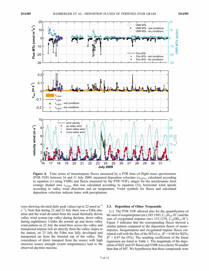
were showing elevated daily peak values (up to 22 nmol m−2

s−1). Note that during 22 and 23 July there was a Föhn situ-ation and the wind deviated from the usual thermally drivenvalley wind system (up valley during daytime, down valleyduring nighttimes). Unlike the normal up and down valleywind pattern on 22 July the wind blew across the valley andtransported terpene rich air directly from the valley slopes tothe station, on 23 July the Föhn was fully developed andtransported air from the forested top of the valley. Thecoincidence of direct transport from the source with highemission source strength (warm temperatures) lead to theobserved daytime maxima.

3.3. Deposition of Other Terpenoids

[21] The PTR‐TOF allowed also for the quantification ofthe sum of sesquiterpenes (m/z 205.1945, C15H24‐H

+) and thesum of oxygenated terpenes (m/z 153.1278, C10OH16‐H

+).Figure 5 indicates that the corresponding fluxes showed asimilar pattern compared to the deposition fluxes of mono-terpenes. Sesquiterpene and oxygenated terpene fluxes cor-related well with the flux of theMTs (i.e., R2 = 0.80 for SQTs;R2 = 0.87 for OTs). The resulting coefficients of the linearregression are listed in Table 1. The magnitude of the depo-sition of SQT andOT fluxes andVMRwas a factor 50 smallerthan that of MT. We hypothesize that these compounds were

Figure 4. Time series of monoterpene fluxes measured by a PTR time‐of‐flight‐mass spectrometer(PTR‐TOF) between 16 and 31 July 2009, measured deposition velocities (vd,MTs, calculated accordingto equation (1) using VMRs and fluxes measured by the PTR‐TOF), ranges for the aerodynamic limit(orange shaded area vd,max that was calculated according to equation (3)), horizontal wind speedsaccording to valley wind directions and air temperature. Violet symbols for fluxes and calculateddeposition velocities indicate times with precipitation.

BAMBERGER ET AL.: DEPOSITION FLUXES OF TERPENES OVER GRASS D14305D14305

7 of 13

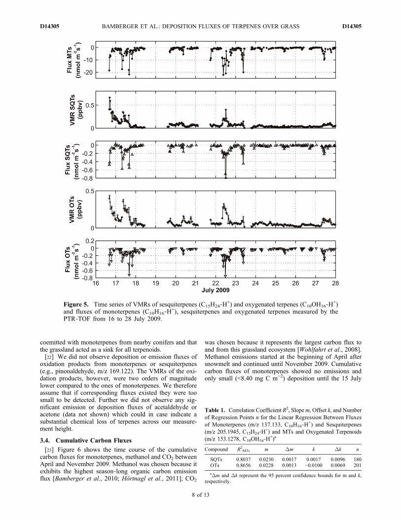
coemitted with monoterpenes from nearby conifers and thatthe grassland acted as a sink for all terpenoids.[22] We did not observe deposition or emission fluxes of

oxidation products from monoterpenes or sesquiterpenes(e.g., pinonaldehyde, m/z 169.122). The VMRs of the oxi-dation products, however, were two orders of magnitudelower compared to the ones of monoterpenes. We thereforeassume that if corresponding fluxes existed they were toosmall to be detected. Further we did not observe any sig-nificant emission or deposition fluxes of acetaldehyde oracetone (data not shown) which could in case indicate asubstantial chemical loss of terpenes across our measure-ment height.

3.4. Cumulative Carbon Fluxes

[23] Figure 6 shows the time course of the cumulativecarbon fluxes for monoterpenes, methanol and CO2 betweenApril and November 2009. Methanol was chosen because itexhibits the highest season‐long organic carbon emissionflux [Bamberger et al., 2010; Hörtnagl et al., 2011]; CO2

was chosen because it represents the largest carbon flux toand from this grassland ecosystem [Wohlfahrt et al., 2008].Methanol emissions started at the beginning of April aftersnowmelt and continued until November 2009. Cumulativecarbon fluxes of monoterpenes showed no emissions andonly small (<8.40 mg C m−2) deposition until the 15 July

Figure 5. Time series of VMRs of sesquiterpenes (C15H24‐H+) and oxygenated terpenes (C10OH16‐H

+)and fluxes of monoterpenes (C10H16‐H

+), sesquiterpenes and oxygenated terpenes measured by thePTR‐TOF from 16 to 28 July 2009.

Table 1. Correlation Coefficient R2, Slopem, Offset k, and Numberof Regression Points n for the Linear Regression Between Fluxesof Monoterpenes (m/z 137.133, C10H16‐H

+) and Sesquiterpenes(m/z 205.1945, C15H24‐H

+) and MTs and Oxygenated Terpenoids(m/z 153.1278, C10OH16‐H

+)a

Compound R2MTs m Dm k Dk n

SQTs 0.8037 0.0230 0.0017 0.0017 0.0096 180OTs 0.8656 0.0228 0.0013 −0.0100 0.0069 201

aDm and Dk represent the 95 percent confidence bounds for m and k,respectively.

BAMBERGER ET AL.: DEPOSITION FLUXES OF TERPENES OVER GRASS D14305D14305

8 of 13

2009 when the onset of the high monoterpene uptake (16 July)was most likely triggered by the above mentioned hailstormwhich damaged needles and twigs of the nearby coniferousforest and elevated the valley VMRs by an order of magnitude.Starting from that point of time cumulative monoterpenedeposition fluxes increased significantly and flattened out onlyslowly before they reached a constant level in October 2009.During periods of cutting and fertilization the methanol curveexhibited abrupt increases because of bursts of emissions fromdamaged vegetation; CO2 fluxes showed a reversal fromuptake to emission and back to uptake which is characteristicfor vegetation recovery after cutting [Wohlfahrt et al., 2008].[24] From April to November 2009, the total amount of

carbon deposited to this grassland in form of monoterpeneswas 276 mg C m−2. This is comparable to the net carbonemissions of methanol (329 mg C m−2, including cutting andfertilization) during the same time period. The net CO2 car-bon uptake over this meadow within the mentioned period oftime was 289 g C m−2. Assuming that during the periodsbetween January and April and November until December nonotable uptake or emission of monoterpenes took place themeasured monoterpene deposition of 0.28 g C m−2 yr−1 isremarkably high when compared to global terpene emissionestimates from forested areas. For example, emission esti-mates for monoterpenes for different temperate forest envir-onments range between 0.42 g C m−2 yr−1 and 0.92 g C m−2

yr−1 [Guenther et al., 1995]. Naik et al. [2004] reported

average emissions of 1.66 g C m−2 yr−1 for temperate ever-green conifer forest and 0.73 g C m−2 yr−1 for temperatedeciduous forest.[25] Goldstein and Galbally [2007] proposed that large

fractions of the emitted BVOCs are removed from theatmosphere by the production of SOA. Our results, however,suggest that gas phase deposition processes could play a moresignificant role than heretofore supposed.

4. Summary and Conclusions

[26] Over a time period of two subsequent years fluxes ofthe sum of monoterpenes were measured above a grasslandin an alpine valley using a PTR‐MS. Fluxes were evaluatedby means of the disjunct eddy covariance method. Withinthe frame of a four month campaign during the second yeara PTR‐TOF was additionally deployed at the field site tostudy complete mass spectra at 10 Hz time resolution forsesquiterpene and oxygenated terpenoid fluxes.[27] VMR measurements suggest that coniferous trees can

emit monoterpenes in large quantities in response to ‘natural’stress conditions (e.g., after a hailstorm) and that, on a localscale, volume mixing ratios can be as large as several ppbv inthe atmosphere. As a consequence of the enhanced volumemixing ratios in the air significant deposition of mono-terpenes to grassland was observed. Deposition of sesqui-terpenes and oxygenated terpenes to the grassland site was

Figure 6. Cumulative carbon fluxes of monoterpenes, methanol, and CO2 calculated from the PTR‐MSand infrared gas analyzer data (gaps shorter or equal to 2 h were filled with interpolated values) for thetime period from 1 April until 1 November 2009. The vertical lines represent the dates of cutting (4 June2009, 5 August 2009, and 21 September 2009) and fertilization (19 October 2009).

BAMBERGER ET AL.: DEPOSITION FLUXES OF TERPENES OVER GRASS D14305D14305

9 of 13

highly correlated with the observed monoterpene fluxes.During dry daytime conditions the observed depositionvelocities were, with values close to the aerodynamic limitcalculated from dry deposition theory, remarkably high. Theuptake of terpenes by grassland lasted for several weekswithout observed reemission. Cumulative carbon depositionfluxes of monoterpenes over grassland can reach the samerange as net carbon emissions of methanol, the dominantBVOC emitted by grasslands.Moreover, the carbon uptake ofmonoterpenes by the grassland reached values which are inthe same order of magnitude as carbon emissions of mono-terpenes by forested areas used in global emission estimates.[28] Our measurements suggest that deposition processes

of monoterpenes could play a more significant role in thereactive carbon budget than previously assumed. Thebroader implications of this study are that bidirectional VOCexchange may occur for many, if not all, compounds. In thelight of our study it may thus be worthwhile to change theterminology from the commonly used VOC emissions toVOC exchange. Finally, our findings should be incorporatedinto models which simulate the exchange of VOC across theecosystem‐atmosphere boundary.

Appendix A: Cross‐Correlation Analysis,Cospectra, and Random Flux Uncertainty

[29] The time shift between the vertical wind velocity andthe monoterpene time series (due to the residence time in thetubing, diverging computer clocks, etc.) was determined bysearching for the maximum/minimum cross correlation in agiven time window. For the PTR‐TOF data this approach wasfurther used to apply a quality rating following Ruuskanenet al. [2011]: Fluxes with a clearly visible covariance maxi-mum or minimum were rated class 1; fluxes with a recog-nizable but uncertain (in peak position) maximum orminimum were rated class 2 (recognizable peak); all otherhalf‐hourly periods were rated class 3 and excluded from theanalysis. Examples for these three quality classes are shownin Figure A1.[30] A cospectral analysis of an exemplary half‐hourly

period (Figure A2) shows that MT cospectra measured withthe PTR‐MS and PTR‐TOF exhibit similar cospectral den-sity at low and intermediate frequencies as compared to

sensible heat cospectra and correspond reasonably well withthe site‐specific cospectral reference model [Wohlfahrtet al., 2005]. Note that the PTR‐MS and PTR‐TOF MTcospectra are characterized by a lower Nyquist frequency ascompared to the sensible heat cospectra, which are acquiredby the sonic anemometer at 20 Hz, due repetition rates of2.3–3 s and 0.1 s, respectively. Because of the disjunctsampling with the PTR‐MS MT cospectra are in additionnoisier [Hörtnagl et al., 2010]. Figure A2 also shows asimulated reference cospectrum that has been attenuated bya series of transfer functions accounting for both low‐ andhigh‐pass filtering of MT fluxes [Bamberger et al., 2010].PTR‐TOF cospectra nicely overlap with the attenuatedmodel cospectrum at higher frequencies, confirming theapproach of accounting for frequency loss [Bambergeret al., 2010]. More than 50% of the MT fluxes were cor-rected with frequency response correction factors of 1.06 orless, 90% with 1.12 or less.[31] The random MT flux uncertainty was calculated

based on measurements under similar environmental con-ditions during adjacent days a suggested by Hollinger andRichardson [2005] using two years of PTR‐MS and twomonths of PTR‐TOF data. Similar environmental conditionswere defined as differences in environmental conditions atthe same time of day between two adjacent days of lessthan: 100 mmol m−2 s−1 incident photosynthetically activeradiation, 2°C air temperature, 1°C soil temperature, 10%relative humidity, 1 m s−1 horizontal wind speed, 0.1 ppbvambient MT mixing ratios. As shown in Figure A3 PTR‐MSflux uncertainties were similar in magnitude for depositionand emission fluxes. As discussed by Hörtnagl et al. [2010],disjunct sampling causes an increase in the random fluxuncertainty, which can be seen for MT deposition fluxes inthe comparison to the fluxes calculated from the 10 HzPTR‐TOF data.

Appendix B: Comparison of Monoterpene Fluxes

[32] Figure B1 shows a comparison between the 12 h day-time monoterpene fluxes calculated from PTR‐MS data andthe corresponding fluxes calculated from the PTR‐TOF data.It can be seen that the PTR‐TOF fluxes tend to be highercompared to the PTR‐MS fluxes but show the same pattern. A

Figure A1. Example for covariance peaks which were rated as (left) class 1, (middle) class 2 and (right)class 3. The black dots represent the measurement points, and the red line is a smoothed line after theapplication of a moving average filter.

BAMBERGER ET AL.: DEPOSITION FLUXES OF TERPENES OVER GRASS D14305D14305

10 of 13

Figure A3. Random MT flux uncertainty for PTR‐MS (solid red circles) and PTR‐TOF (open greencircles) measurements determined according to the method of Hollinger and Richardson [2005]. Datahave been binned into classes of equal size; error bars represent ±1 standard deviation. A double‐linearrelationship with a common y intercept was fit to the PTR‐MS data: y = 0.51x + 0.07 (emission), y =−0.58x + 0.07 (deposition), R2 = 0.92. For the PTR‐TOF data not enough emission fluxes were capturedso that flux uncertainties have been calculated only for deposition fluxes (y = −0.46x + 0.04, R2 = 0.93).

Figure A2. Comparison of exemplary cospectra for the sensible heat (blue dots) and MT (red trianglesfor the PTR‐MS and black triangles for the PTR‐TOF) flux together with the cospectral referencemodel (solid line) [Wohlfahrt et al., 2005] and the reference model attenuated by a series of transferfunctions which account for low‐ and high‐pass filtering of the MT flux (dashed line). Cospectra havebeen obtained on 22 July 2009 09:00–09:30 under the following conditions: average horizontal windspeed, 0.2 m s−1; Monin‐Obukov stability parameter, −0.1. Note the lower Nyquist frequency for thePTR‐MS and PTR‐TOF MT cospectra due repetition rates of 2.3–3 s and 10 Hz compared to the 20 Hzof the sonic anemometer.

BAMBERGER ET AL.: DEPOSITION FLUXES OF TERPENES OVER GRASS D14305D14305

11 of 13

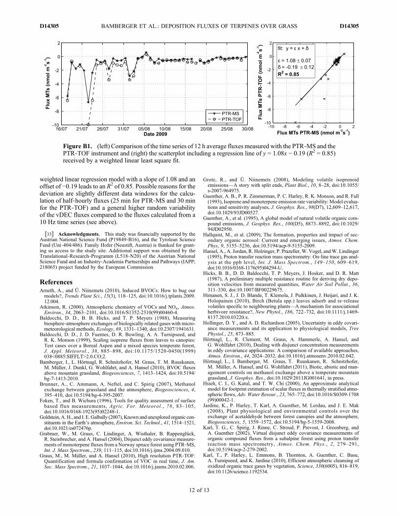
weighted linear regression model with a slope of 1.08 and anoffset of −0.19 leads to an R2 of 0.85. Possible reasons for thedeviation are slightly different data windows for the calcu-lation of half‐hourly fluxes (25 min for PTR‐MS and 30 minfor the PTR‐TOF) and a general higher random variabilityof the vDEC fluxes compared to the fluxes calculated from a10 Hz time series (see above).

[33] Acknowledgments. This study was financially supported by theAustrian National Science Fund (P19849‐B16), and the Tyrolean ScienceFund (Uni‐404/486). Family Hofer (Neustift, Austria) is thanked for grant-ing us access to the study site. Additional support was obtained by theTranslational‐Research‐Programm (L518‐N20) of the Austrian NationalScience Fund and an Industry‐Academia Partnerships and Pathways (IAPP;218065) project funded by the European Commission.

ReferencesArneth, A., and Ü. Niinemets (2010), Induced BVOCs: How to bug ourmodels?, Trends Plant Sci., 15(3), 118–125, doi:10.1016/j.tplants.2009.12.004.

Atkinson, R. (2000), Atmospheric chemistry of VOCs and NOx, Atmos.Environ., 34, 2063–2101, doi:10.1016/S1352-2310(99)00460-4.

Baldocchi, D. D., B. B. Hicks, and T. P. Meyers (1988), Measuringbiosphere‐atmosphere exchanges of biologically related gases with micro-meteorological methods, Ecology, 69, 1331–1340, doi:10.2307/1941631.

Baldocchi, D. D., J. D. Fuentes, D. R. Bowling, A. A. Turnipseed, andR. K. Monson (1999), Scaling isoprene fluxes from leaves to canopies:Test cases over a Boreal Aspen and a mixed species temperate forest,J. Appl. Meteorol., 38, 885–898, doi:10.1175/1520-0450(1999)038<0885:SIFFLT>2.0.CO;2.

Bamberger, I., L. Hörtnagl, R. Schnitzhofer, M. Graus, T. M. Ruuskanen,M. Müller, J. Dunkl, G. Wohlfahrt, and A. Hansel (2010), BVOC fluxesabove mountain grassland, Biogeosciences, 7, 1413–1424, doi:10.5194/bg-7-1413-2010.

Brunner, A., C. Ammann, A. Neftel, and C. Spirig (2007), Methanolexchange between grassland and the atmosphere, Biogeosciences, 4,395–410, doi:10.5194/bg-4-395-2007.

Foken, T., and B. Wichura (1996), Tools for quality assessment of surfacebased flux measurements, Agric. For. Meteorol., 78 , 83–105,doi:10.1016/0168-1923(95)02248-1.

Goldstein,A.H., and I. E. Galbally (2007), Known and unexplored organic con-stituents in the Earth’s atmosphere, Environ. Sci. Technol., 41, 1514–1521,doi:10.1021/es072476p.

Grabmer, W., M. Graus, C. Lindinger, A. Wisthaler, B. Rappenglück,R. Steinbrecher, and A. Hansel (2004), Disjunct eddy covariance measure-ments of monoterpene fluxes from a Norway spruce forest using PTR‐MS,Int. J. Mass Spectrom., 239, 111–115, doi:10.1016/j.ijms.2004.09.010.

Graus, M., M. Müller, and A. Hansel (2010), High resolution PTR‐TOF:Quantification and formula confirmation of VOC in real time, J. Am.Soc. Mass Spectrom., 21, 1037–1044, doi:10.1016/j.jasms.2010.02.006.

Grote, R., and Ü. Niinemets (2008), Modeling volatile isoprenoidemissions—A story with split ends, Plant Biol., 10, 8–28, doi:10.1055/s-2007-964975.

Guenther, A. B., P. R. Zimmerman, P. C. Harley, R. K. Monson, and R. Fall(1993), Isoprene andmonoterpene emission rate variability:Model evalua-tions and sensitivity analyses, J. Geophys. Res., 98(D7), 12,609–12,617,doi:10.1029/93JD00527.

Guenther, A., et al. (1995), A global model of natural volatile organic com-pound emissions, J. Geophys. Res., 100(D5), 8873–8892, doi:10.1029/94JD02950.

Hallquist, M., et al. (2009), The formation, properties and impact of sec-ondary organic aerosol: Current and emerging issues, Atmos. Chem.Phys, 9, 5155–5236, doi:10.5194/acp-9-5155-2009.

Hansel, A., A. Jordan, R. Holzinger, P. Prazeller, W. Vogel, andW. Lindinger(1995), Proton transfer reaction mass spectrometry: On‐line trace gas anal-ysis at the ppb level, Int. J. Mass Spectrom., 149–150, 609–619,doi:10.1016/0168-1176(95)04294-U.

Hicks, B. B., D. D. Baldocchi, T. P. Meyers, J. Hosker, and D. R. Matt(1987), A preliminary multiple resistance routine for deriving dry depo-sition velocities from measured quantities, Water Air Soil Pollut., 36,311–330, doi:10.1007/BF00229675.

Himanen, S. J., J. D. Blande, T. Klemola, J. Pulkkinen, J. Heijari, and J. K.Holopainen (2010), Birch (Betula spp.) leaves adsorb and re‐releasevolatiles specific to neighbouring plants—A mechanism for associationalherbivore resistance?, New Phytol., 186, 722–732, doi:10.1111/j.1469-8137.2010.03220.x.

Hollinger, D. Y., and A. D. Richardson (2005), Uncertainty in eddy covari-ance measurements and its application to physiological models, TreePhysiol., 25, 873–885.

Hörtnagl, L., R. Clement, M. Graus, A. Hammerle, A. Hansel, andG. Wohlfahrt (2010), Dealing with disjunct concentration measurementsin eddy covariance applications: A comparison of available approaches,Atmos. Environ., 44, 2024–2032, doi:10.1016/j.atmosenv.2010.02.042.

Hörtnagl, L., I. Bamberger, M. Graus, T. Ruuskanen, R. Schnitzhofer,M. Müller, A. Hansel, and G. Wohlfahrt (2011), Biotic, abiotic and man-agement controls on methanol exchange above a temperate mountaingrassland, J. Geophys. Res., doi:10.1029/2011JG001641, in press.

Hsieh, C. I., G. Katul, and T. W. Chi (2000), An approximate analyticalmodel for footprint estimation of scalar fluxes in thermally stratified atmo-spheric flows, Adv. Water Resour., 23, 765–772, doi:10.1016/S0309-1708(99)00042-1.

Jardine, K., P. Harley, T. Karl, A. Guenther, M. Lerdau, and J. E. Mak(2008), Plant physiological and environmental controls over theexchange of acetaldehyde between forest canopies and the atmosphere,Biogeosciences, 5, 1559–1572, doi:10.5194/bg-5-1559-2008.

Karl, T. G., C. Spirig, J. Rinne, C. Stroud, P. Prevost, J. Greenberg, andA. Guenther (2002), Virtual disjunct eddy covariance measurements oforganic compound fluxes from a subalpine forest using proton transferreaction mass spectrometry, Atmos. Chem. Phys., 2, 279–291,doi:10.5194/acp-2-279-2002.

Karl, T., P. Harley, L. Emmons, B. Thornton, A. Guenther, C. Basu,A. Turnipseed, and K. Jardine (2010), Efficient atmospheric cleansing ofoxidized organic trace gases by vegetation, Science, 330(6005), 816–819,doi:10.1126/science.1192534.

Figure B1. (left) Comparison of the time series of 12 h average fluxes measured with the PTR‐MS and thePTR‐TOF instrument and (right) the scatterplot including a regression line of y = 1.08x − 0.19 (R2 = 0.85)received by a weighted linear least square fit.

BAMBERGER ET AL.: DEPOSITION FLUXES OF TERPENES OVER GRASS D14305D14305

12 of 13

Kesselmeier, J. (2001), Exchange of short‐chain oxygenated volatileorganic compounds (VOCs) between plants and the atmosphere: A com-pilation of field and laboratory studies, J. Atmos. Chem., 39, 219–233,doi:10.1023/A:1010632302076.

Kesselmeier, J., and M. Staudt (1999), Biogenic volatile organic compounds(VOC): An overview on emission, physiology and ecology, J. Atmos.Chem., 33, 23–88, doi:10.1023/A:1006127516791.

Kirstine, W., I. Galbally, Y. Ye, and M. Hooper (1998), Emissions ofvolatile organic compounds (primarily oxygenated species) from pasture,J. Geophys. Res., 103(D9), 10,605–10,619, doi:10.1029/97JD03753.

Lindinger, W., A. Hansel, and A. Jordan (1998), On‐line monitoring ofvolatile organic compounds at pptv levels by means of proton‐transfer‐reaction mass spectrometry (PTR‐MS) medical applications, food controland environmental research, Int. J. Mass Spectrom., 173, 191–241,doi:10.1016/S0168-1176(97)00281-4.

Liu, S., L. Lu, D. Mao, and J. Lia (2007), Evaluating parameterizations ofaerodynamic resistance to heat transfer using field measurements,Hydrol. Earth Syst. Sci., 11, 769–783, doi:10.5194/hess-11-769-2007.

Loreto, F., P. Nascetti, A. Graverini, and M. Mannozzi (2000), Emissionand content of monoterpenes in intact and wounded needles of the Med-iterranean Pine, Pinus pinea, Funct. Ecol., 14, 589–595, doi:10.1046/j.1365-2435.2000.t01-1-00457.x.

McMillen, R. T. (1988), An eddy correlation technique with extendedapplicability to non‐simple terrain, Boundary Layer Meteorol., 43,231–245, doi:10.1007/BF00128405.

Monteith, J. L., and M. H. Unsworth (1990), Principles of EnvironmentalPhysics, 2nd ed., 291 pp., Edward Arnold, New York.

Müller, M., et al. (2010), First eddy covariance flux measurements byPTR‐TOF, Atmos. Meas. Tech., 3, 387–395, doi:10.5194/amt-3-387-2010.

Naik, V., C. Delire, and D. J. Wuebbles (2004), Sensitivity of globalbiogenic isoprenoid emissions to climate variability and atmosphericCO2, J. Geophys. Res., 109, D06301, doi:10.1029/2003JD004236.

Niinemets, Ü., F. Loreto, and M. Reichstein (2004), Physiological andphysicochemical controls on foliar volatile organic compound emissions,Trends Plant Sci., 9(4), 180–186, doi:10.1016/j.tplants.2004.02.006.

Noe, S. M., L. Copolovici, Ü. Niinemets, and E. Vaino (2008), Foliar lim-onene uptake scales positively with leaf lipid content: “Non‐emitting”species absorb and release monoterpenes, Plant Biol., 10, 129–137,doi:10.1055/s-2007-965239.

Novick, K. A., P. C. Stoy, G. G. Katul, D. S. Ellsworth, M. B. S. Siqueira,J. Juang, and R. Oren (2004), Carbon dioxide and water vapor exchangein a warm temperate grassland, Oecologia, 138, 259–274, doi:10.1007/s00442-003-1388-z.

Potter, C. S., S. E. Alexander, J. C. Coughlan, and S. A. Klooster (2001),Modeling biogenic emissions of isoprene: Exploration of model drivers,

climate control algorithms, and use of global satellite observations,Atmos. Environ., 35, 6151–6165, doi:10.1016/S1352-2310(01)00390-9.

Rinne, J., R. Taipale, T. Markkanen, T. M. Ruuskanen, H. Hellén, M. K.Kajos, T. Vesala, and M. Kulmala (2007), Hydrocarbon fluxes above aScots pine forest canopy: Measurements and modeling, Atmos. Chem.Phys., 7, 3361–3372, doi:10.5194/acp-7-3361-2007.

Ruuskanen, T.M.,M.Müller, R. Schnitzhofer, T. Karl,M.Graus, I. Bamberger,L. Hörtnagl, F. Brilli, G. Wohlfahrt, and A. Hansel (2011), Eddy covarianceVOC emission and deposition fluxes above grassland using PTR‐TOF,Atmos. Chem. Phys., 11, 611–625, doi:10.5194/acp-11-611-2011.

Spirig, C., A. Neftel, C. Ammann, J. Dommen, W. Grabmer, A. Thielmann,A. Schaub, J. Beauchamp, A. Wisthaler, and A. Hansel (2005), Eddycovariance flux measurements of biogenic VOCs during ECHO 2003using proton transfer reaction mass spectrometry, Atmos. Chem. Phys.,5, 465–481, doi:10.5194/acp-5-465-2005.

Wesely,M.L., andB.B.Hicks (2000), A reviewof the current status of knowl-edge on dry deposition, Atmos. Environ., 34, 2261–2282, doi:10.1016/S1352-2310(99)00467-7.

Wohlfahrt, G., S. Sapinsky, U. Tappeiner, and A. Cernusca (2001), Estima-tion of plant area index of grasslands from measurements of canopy radi-ation profiles, Agric. For. Meteorol., 109, 1–12, doi:10.1016/S0168-1923(01)00259-3.

Wohlfahrt, G., C. Anfang, M. Bahn, A. Haslwanter, C. Newesely,M. Schmitt, M. Drösler, J. Pfadenhauer, and A. Cernusca (2005), Quanti-fying nighttime ecosystem respiration of a meadow using eddy covariance,chambers and modelling, Agric. For. Meteorol., 128, 141–162,doi:10.1016/j.agrformet.2004.11.003.

Wohlfahrt, G., A. Hammerle, A. Haslwanter, M. Bahn, U. Tappeiner, andA. Cernusca (2008), Seasonal and inter‐annual variability of the net eco-system CO2 exchange of a temperate mountain grassland: Effects ofweather and management, J. Geophys. Res., 113, D08110, doi:10.1029/2007JD009286.

I. Bamberger, A. Hansel,M.Müller, T.M. Ruuskanen, and R. Schnitzhofer,Institute of Ion Physics and Applied Physics, University of Innsbruck,Technikerstraße 25, A‐6020 Innsbruck, Austria. (armin.hansel@uibk.ac.at)M. Graus, Chemical Sciences Division, Earth System Research Laboratory,

NOAA, 325 Broadway, Boulder, CO 80305‐3337, USA.L.Hörtnagl andG.Wohlfahrt, Institute of Ecology,University of Innsbruck,

Sternwartestraße 15, A‐6020 Innsbruck, Austria.T. Karl, Earth Systems Laboratory, NCAR, PO Box 3000, Boulder, CO

80307, USA.

BAMBERGER ET AL.: DEPOSITION FLUXES OF TERPENES OVER GRASS D14305D14305

13 of 13