ARTICLE IN PRESS

Neurocomputing 72 (2009) 2682–2692

Contents lists available at ScienceDirect

Neurocomputing

0925-23

doi:10.1

� Corr

E-m

journal homepage: www.elsevier.com/locate/neucom

Dependent component analysis for blind restoration of images degraded byturbulent atmosphere

Qian Du a,�, Ivica Kopriva b

a Department of Electrical and Computer Engineering, Mississippi State University, Mississippi State, MS 39762, USAb Division of Laser and Atomic Research and Development, Rudjer Boskovic Institute, Bijenicka cesta 54, PO Box 180, 10002 Zagreb, Croatia

a r t i c l e i n f o

Article history:

Received 31 March 2008

Received in revised form

29 August 2008

Accepted 28 September 2008

Communicated by S. Choipaper, we propose to apply the concept of dependent component analysis (DCA), which can relax the

Available online 1 November 2008

Keywords:

Atmospheric turbulence

Image restoration

Independent component analysis

Dependent component analysis

12/$ - see front matter & 2008 Elsevier B.V. A

016/j.neucom.2008.09.012

esponding author. Tel.: 662 325 2035; fax: 66

ail address: du@ece.msstate.edu (Q. Du).

a b s t r a c t

In our previous research, we applied independent component analysis (ICA) for the restoration of image

sequences degraded by atmospheric turbulence. The original high-resolution image and turbulent

sources were considered independent sources from which the degraded image is composed of. Although

the result was promising, the assumption of source independence may not be true in practice. In this

independence assumption, to image restoration. In addition, the restored image can be further

enhanced by employing a recently developed Gabor-filter-bank-based single channel blind image

deconvolution algorithm. Both simulated and real data experiments demonstrate that DCA outperforms

ICA, resulting in the flexibility in the use of adjacent image frames. The contribution of this research is to

convert the original multi-frame blind deconvolution problem into blind source separation problem

without the assumption on source independence; as a result, there is no a priori information, such as

sensor bandwidth, point-spread-function, or statistics of source images, that is required.

& 2008 Elsevier B.V. All rights reserved.

1. Introduction

Atmospheric turbulence is an inevitable problem in long-distance ground-based and space-based imaging. The opticaleffects of atmospheric turbulence arise from random inhomo-geneities in the temperature distribution of the atmosphere.A consequence of these temperature inhomogeneities is non-stationary random distribution of the refraction index of theatmosphere [30]. Atmospheric turbulence can make distantobjects being viewed through a sensor (e.g., a digital camera orvideo recorder) to appear blurred. Also, the time-varying nature ofthe turbulence can make the appearance of objects to wave in aslow quasi-periodic fashion. When a target is small and moving,its actual location becomes very difficult to estimate. Thisphenomenon greatly hinders accurate target detection, tracking,classification, and identification.

Numerous methods have been developed to mitigate theatmospheric turbulence effects. Three broad classes of techniquesused to correct turbulence effects are: (1) pure post-processingtechniques, which use specialized image processing algorithms;(2) adaptive optics techniques, which afford a mechanical meansof sensing and correcting for turbulence effects; and (3) hybrid

ll rights reserved.

2 325 2298.

methods, which combine the elements of post-processing tech-niques and adaptive optics techniques. Each of these techniqueshas performance limitation as well as hardware and softwarerequirements. In our research, due to its low cost, we focus on thedevelopment of pure post-processing techniques to correctatmospheric turbulence. Quite a few algorithms in this aspecthave been developed in the past 20 years. These algorithms fallinto two major categories: those adopting explicit or implicit waysto measure the perturbations induced on the wavefront by theatmosphere, and those using no wavefront information toconstruct the underlying image formation characteristics of theatmosphere. Wavefront reference algorithms include the guides(natural or artificial) and deconvolution from optical measure-ments of the wavefront entering the telescope, while reference-less algorithms do not need such guides. In our research, we areinterested in the no-reference techniques because no opticalmeasurements are required. This also makes real-time or near-real-time implementation possible and simple for many nationaldefense-related applications.

Current image restoration techniques for atmospheric turbu-lence correction employ the well-known linear image formationmodel g(x,y) ¼ h(x,y)*s(x,y), where the degraded image g(x,y) isobtained by convolving the original high-resolution image s(x,y)with the point-spread-function (PSF) h(x,y) (i.e., PSF modelsthe degradation caused by atmospheric turbulence) [27]. Due tothe space- and time-varying nature of atmospheric turbulence,

ARTICLE IN PRESS

Q. Du, I. Kopriva / Neurocomputing 72 (2009) 2682–2692 2683

the PSF should be changed with pixel location (x,y) and time t.However, for the purpose of simplicity and mathematical tract-ability, most techniques assume that PSF is unchanged with spaceand time. In other words, they are space- and time-invariantrestoration approaches.

To relax the unrealistic assumption of a space- and time-invariant PSF, we introduced the blind source separation (BSS)technique to achieve the restoration of image sequences [22].Instead of using the linear convolutive degradation model andestimating the PSF, we considered each spatial turbulence patternas one physical source, the original high-resolution image of theobject as another source, and then the degraded low-resolutionimage was the result from the linear combination of these sources.This leads to the model at the component level written as

gðx; y; tnÞ ¼XMm¼1

anmðDtnÞsmðx; y; t0Þ (1)

where contributions from the high-resolution object image andthe individual turbulence patterns {Sm}m ¼ 1

M between time tn andthe reference time t0, i.e. Dtn ¼ tn�t0, are contained in theunknown mixing matrix coefficients anm, which depend on somephysical constants [22]. The component level model (1) can begeneralized to a multi-frame model in a matrix form as

G ¼ AS (2)

where GARN� T is a matrix of the blurred image frames with eachrow representing a blurred image frame, AARN�M is an unknownbasis or mixing matrix, and SARN� T is a matrix of the sourceimages. Here, N represents the number of frames whereas eachframe is treated as one measurement, M denotes the number ofsource images, and T ¼ P�Q stands for the number of pixels ineach image (P and Q are image spatial dimensions). It is assumedthat each image frame has been transformed into a vector by arow or column stacking procedure. It is also assumed that motioneffects, if present, are compensated in advance.

Intuitively, the more sources associated with the turbulencephenomenon are included, the better quality of the restoredimage is expected. The reason is that turbulence effects aresubtracted from the degraded images in the linear demixingprocess. Thus, the overall number of sources, M, is set to equal theoverall number of frames (i.e. measurements). This is then in theagreement with the known fact that the quality of a restoredimage in multi-frame image restoration generally is increasedwhen the number of frames is increased.

BSS can be applied on (2) to extract the high-resolution objectimage without the prior knowledge or estimation of PSF. The mostsuccessful solution of the BSS problem is achieved throughindependent component analysis (ICA). It solves the BSS problemby imposing a constraint on extracted sources to be non-Gaussian(at most one source is allowed to be Gaussian) and statisticallyindependent from each other [16]. One of popular ICA algorithms,referred to as Joint Approximate Dia-gonalization of Eigenma-trices (JADE), was adopted due to its robustness, wherein thestatistical dependence among data samples was measured by thefourth-order cross-cumulants [5].

However, it has been argued that the assumption of sourceindependence may not be true in many situations. For instance,the atmospheric turbulence components may be correlatedspatially and temporally. Sources may be at least partiallystatistically dependent due to the fact that multi-frame imagemodel adopted in [22] and used herein assumes all the sources areemitted from the same space-time location (x, y, t0). Thus, in thispaper, we will propose the use of dependent component analysis(DCA) for image restoration, which does not require sourcesto be independent. Both simulated and real data experiments

demonstrate that DCA outperforms ICA under this circumstance.In addition, DCA can be employed to further sharpen the restoredimage to achieve super-resolution.

In summary, the contribution of this research is to convert theoriginal multi-frame blind deconvolution problem into BSSproblem without the assumption on source independence; as aresult, no a priori information or assumption on sensor band-width, PSF, or statistics of source images is required.

2. Derivation of DCA algorithms

Few papers in the literature discuss the problem of DCA [1].Here we adopt some previous studies conducted in [18,21]. Thebasic idea behind DCA is to find a transform T that can improvethe statistical independence between the sources but leave thebasis matrix unchanged, i.e.,

TðGÞ ¼ TðASÞ ffi ATðSÞ (3)

Because the sources after this transformation will be lessstatistically dependent, any standard ICA algorithm, such as JADE,derived for the original BSS problem can be used to learn the basismatrix A. Once the basis matrix A is estimated, the sources S canbe recovered by applying the pseudo-inverse of A on the multi-frame image G in (2).

Examples of linear transforms that possess such a requiredinvariance property and generate less dependent sources include:(1) highpass filtering, (2) innovation, and (3) wavelet transforms.

2.1. Highpass filtering (HP)

A highpass filter, such as the Butterworth highpass filter, isapplied to preprocess the observed signals G, followed by astandard ICA algorithm, such as JADE, on the filtered data in orderto learn the mixing matrix A. This is motivated by the fact thathighpass filtered signals are usually more independent thanoriginal signals that include low frequency components. Mean-while, this approach is computationally very efficient, making itattractive for DCA problems with statistically dependent sources.In this case, the transform T in Eq. (3) is the HP operator that canbe seen as a special case of the filter bank approach [6,36].

2.2. Innovation (IN)

Another computationally efficient approach is based on the useof innovation. The arguments for using innovation are that theyare usually more independent from each other and more non-Gaussian than original processes [13]. The innovation process isreferred to as prediction error [26], which is defined as

emðrÞ ¼ smðrÞ �Xl

i¼1

bismðr � iÞ; m ¼ 1; . . . ;M (4)

where sm(r�i) is the i-th sample of a source process sm(r) atlocation (r�i) and b’s are prediction coefficients. em(r) representsthe new information that sm(r) has but is not contained in the pastl samples. It is proved in [13] that if G and S follow the linearmixture model (2) their innovation processes EG and ES (in matrixform) follow the same model as well, i.e.,

EG ¼ AES (5)

In this case, the transform T in Eq. (3) is the linear predictionoperator. Temporal decorrelation-based preprocessing algorithm[15] can be seen as an extension of the presented innovation-based DCA algorithm. It is the same as the presented method

ARTICLE IN PRESS

Q. Du, I. Kopriva / Neurocomputing 72 (2009) 2682–26922684

when the model is linear but the algorithm in [15] works in thecase of post-nonlinear mixture as well.

2.3. Sub-band decomposition independent component

analysis (SDICA)

The SDICA approach assumes that wideband source signals canbe dependent but some of their narrowband sub-components areless dependent [6,36]. Thus, SDICA extends applicability ofstandard ICA through the relaxation of the independenceassumption. In this case, the transform T in Eq. (3) is any kindof filter-bank-like transform used to implement the sub-banddecomposition scheme.

A wavelet transform-based approach to SDICA was developedin [21,19] to obtain adaptive sub-band decomposition of widebandsignals through a computationally efficient implementation in aform of iterative filter bank. Computationally efficient smallcumulant-based approximation of mutual information is usedfor automated selection of the sub-band with the least-dependentcomponents, to which an ICA algorithm is applied. The potentialdisadvantage of this approach is high-computational complexity if2D wavelet transform is used for image decomposition. Hence, areformulation can be accomplished based on dual tree complexwavelets [20]. Dual tree complex wavelets are approximatelycomputationally as efficient as decimated wavelet packets but asaccurate as the shift-invariant wavelet packet approach [17,33].

3. Algorithms for comparison

Other BSS approaches that can deal with statisticallydependent sources include: independent subspace analysis (ISA)[4,14], nonnegative matrix and tensor factorization (NMF/NTF)[24,7–9], and the blind Richardson–Lucy (BRL) algorithm[29,25,10,2], which are used for comparison purpose in this paper.They are briefly described as follows.

3.1. Independent subspace analysis

ISA assumes that the source signal space is composed of anumber of subspaces. Signals contained in the same subspace aremutually dependent while signals contained in different sub-spaces are independent. When each subspace contains onecomponent only, the ISA becomes ICA. The practical difficultywith the ISA approach is in choosing a scheme necessary topartition the source signal space into the subspaces with therequired property. For instance, it is not obvious how to choosethe number of subspaces as well as the number of signalscontained in each subspace.

In the multi-frame blind deconvolution problem treated in thispaper we decompose the signal space into two subspaces:one that contains one image representing an approximation ofthe object and the other that contains images related to theturbulence patterns. Here, we present in the sequel briefderivation of the ISA algorithm [14], which is based on theconcept of multi-dimensional ICA [4] that follows the same modelin (2). It is assumed that components {Sm}m ¼ 1

M are divided into K

tuples where components contained in the same tuple aredependent and components contained in different tuples areindependent (in other words, tuples correspond to subspaces). Itis also assumed in [14] that the joint probability density function(PDF) of a particular subspace is spherically symmetric; hence, itcan be expressed as the sum of squares of fsk

i gdk

i¼1, where k denotesthe subspace index and dk denotes the dimension of the kthsubspace such that

Pk ¼ 1

K dk ¼ M. It is further assumed sparse

representation, which may be in agreement with data representa-tion adopted in our approach due to the fact that turbulencepatterns are expected to be sparse. Under these assumptions thefollowing gradient update for de-mixing matrix W is obtained(i.e., WGES)

DwmðtÞ / �zðtÞsmðtÞX

i2SkðmÞ

ðsiðtÞÞ2

0@

1A�1=2

m ¼ 1; :::;M (6)

where k(m) denotes the index of the subspace to which wm

belongs and z denotes the whitened data (whitening is applied todata matrix in ISA in the same way as in standard ICA) [12].

3.2. Nonnegative matrix and tensor factorization

Unlike ICA, NMF/NTF algorithms do not impose statisticalindependence or non-Gaussianity requirements on the sources.NMF/NTF algorithms may yield physically useful solutions byimposing the non-negativity, sparseness or smoothness con-straints on the sources [24,7–9]. In [24], the NMF algorithm wasfirst derived to minimize two cost functions: the squaredEuclidean distance and the Kullback–Leibler divergence. Using agradient descent approach the resulting multiplicative algorithmsconverged very slowly. In addition, the lack of additionalconstraints prevents NMF algorithms [24] from yielding a uniquedecomposition. Generalization of the NMF algorithms [24]has been done in [7–9]. The gradient-based NMF algorithmwith a sparseness constraint being incorporated into the costfunction leads to the regularized alternating least-square (RALS)algorithm [7]

DðGkASÞ ¼1

2kG� ASk2 þ aSFSðSÞ þ aAFAðAÞ (7)

where the regularization terms aS and aA enforce sparse solutionsfor A and S, respectively. If constraints are chosen as [FS(S)]ij ¼ 1/2sij

2 and [FA(A)]ij ¼ 1/2aij2, the regularization terms help regular-

ize the pseudo-inverse when the normal matrices ATA and SST areill-conditioned. Assume rSD(GJAS) ¼ 0 and rAD(GJAS) ¼ 0 forpositive entries in A and S, which occurs at stationary points. Then

Sðkþ1Þ¼maxf�; ðAT Aþ aðkÞS Þ

þAT GgjA¼AðkÞ

Aðkþ1Þ¼maxf�;GST

ðSSTþ aðkÞA Þ

þgjS¼Sðkþ1Þ (8)

where k denotes iteration index, ()+ is Moore–Penrose inverse, ande is a small constant (10�9) to enforce positive entries. Regular-ization terms help avoid local minima and are implemented asaA(k) ¼ aS(k) ¼ a0exp(�k/t) (in the experiments a0 ¼ 20 andt ¼ 10). We employ constraints if there is a priori informationabout the sparseness of either A or S; otherwise, we set bothregularization terms to zero. This algorithm is referred to as theNMF algorithm in this paper.

Extension of this approach, known as local ALS, to 3D tensorfactorization is given in [8], which is referred to as the NTFalgorithm in this paper. In this case, G and S in model (2) become3D tensors: GAR0+

N� P�Q and SAR0+M� P�Q. Unlike a majority of NTF/

NMF algorithms that estimate the source matrix/tensor globally,the local ALS algorithm [8] performs it at the source level

fsm ¼ ½aTmGðmÞ � aðmÞs �þg

Mm¼1

A ¼ ½A� ðAS� GÞSTðSSTþ lIMÞ

�1�þ (9)

where IM is an M�M identity matrix, as(m) is a sparseness

constraint that regulates sparseness of the mth source, am

represents the mth column of A , G(m)¼ G�

Pjamajsj, and

[x]+ ¼ max{e,x} (e.g., x ¼ 10�16). Regularization constant lchanges as a function of the iteration index as lk ¼ l0exp(�k/t)

ARTICLE IN PRESS

Q. Du, I. Kopriva / Neurocomputing 72 (2009) 2682–2692 2685

(with l0 ¼ 100 and t ¼ 0.02 in the experiments). Note thatsparseness constraint as

(m) imposed on source tensors affectsthe final result (as

(m)¼ 0.05 in the experiment).

3.3. BRL algorithm

BRL algorithm [29,25] was originally derived for non-blindsingle frame deconvolution of astronomical images. It has beenlater formulated in [10] for blind deconvolution, and thenmodified by an iterative restoration algorithm in [2]. To brieflyintroduce BRL algorithm we need to write a single frame image gn,nA{1,y,N}, in the lexicographical notation:

gn ¼ Hs (10)

where gn,sAR0+PQ,HAR0+

PQ� PQ (BRL needs to employ a PSF functionwhose matrix version is H). The observed image vector gn and theoriginal image vector s are obtained by a stacking procedure.The matrix H is a block-Toeplitz matrix [23]. It absorbs itself intothe blurring kernel h(x,y) by assuming that at least its size isknown. The block-Toeplitz structure of H can be furtherapproximated by a block-circular structure. This approximationintroduces small degradations at image boundaries, but enablesthe expression of Eq. (10) with the circular convolution. Thealgorithm can be implemented in the block adaptive fashion

HðkÞ

iþ1 ¼ ½ðsðk�1ÞÞTðg+ðH

k

i sðk�1ÞÞÞ�H

ðkÞ

i

sðkÞiþ1 ¼ ½s

ðkÞi � ðH

ðkÞTðg+ðHðkÞs

ðkÞi ÞÞÞ� (11)

where � denotes component-wise multiplication, + denotescomponent-wise division, i and k are internal and main iterationindices, respectively. Note that although H is blindly estimatedfrom the observed image, its size must be either known orestimated a priori.

4. DCA for single image enhancement

After a high-resolution frame is reconstructed, its quality canbe further improved using a sharpening approach in a post-processing step. In general, it is difficult to conduct imagesharpening based on a single-frame image only, due to the lackof additional information. It is easier if more observations areavailable about the scene, and image details can be extracted fromthese observations. Here, we investigate a single-frame multi-channel image enhancement approach [19]. A 2D Gabor filterbank can be employed to realize multi-channel filtering, con-sidered as multiple observations for ICA or DCA [19]. After themulti-channel version of the original image is generated, an ICA orDCA algorithm can be applied to extract an enhanced image. Themulti-channel linear mixture model of an observed image, in theform of (2), has in [19] been obtained under a special assumptionthat source signals are the original high-resolution source imageand its higher order spatial derivatives. Note that this special classof sources is mutually statistically dependent, [28], DCA algorithmis a better choice than an ICA algorithm to fulfill imageenhancement.

5. No-reference image quality assessment

In order to objectively evaluate image quality after restoration,automatic assessment is needed. When desired high-resolutionimage is available, quality assessment can simply be achieved bycomparing the restored image with desired image using a certaincriterion, such as signal-to-noise ratio (SNR). However, in manypractical situations the desired image is not available. Thus,

quality assessment becomes ‘‘no-reference’’. Here we introducetwo ‘‘no-reference’’ metrics: the area under the magnitude of theone-dimensional (1D) the Fourier transform along a chosen line inthe image and the Laplacian operator.

The power spectrum-based image quality metric has beenproposed in [11,32] due to the invariance of power spectra ofarbitrary scenes. It has been proposed as a substitute for thesubjective image assessment in situations when naturally occur-ring targets are not available and when re-imaging of the samescene for comparison purpose (via mean square error) is notpossible. Most importantly the power spectrum metric can beeasily incorporated into a human visual system model [11,32]. Inthis paper, instead of calculating power spectrum-based imagequality metric in an absolute sense, we compare 1D powerspectrums of images restored by various algorithms. When thepower spectrum is normalized to unit gain at the DC component,the area under it corresponds to the level of details contained inthe image

PSA ¼XOo¼0

jFðoÞjjFð0Þj

(12)

where O corresponds with half of the sampling frequency and|F(o)| represents magnitude of the discrete Fourier transform(DFT) of a chosen line in the image. An image with better qualityof restored details should have a larger PSA.

The Laplacian operator is an approximation to the secondderivative of brightness I(x,y) in direction x and y, can be applied

r2Iðx; yÞ ¼qI2ðx; yÞ

qx2þqI2ðx; yÞ

qy2(13)

It is actually a spatial highpass filter. It yields a larger responseto a point than to a line. An image with turbulence is typicallycomprised of points varying in brightness, and the Laplacianoperator will emphasize these points. A metric based on Laplacianoperator is [31]

I4 ¼ meanðjr2Iðx; yÞjÞ (14)

which takes the average of second-order derivatives of pixels inthe entire image. An image with better quality should have asmaller I4.

PSA emphasizes the details of the restored image, whileLaplacian operator measures the smoothness of the restoredimage. A successful image restoration process should simulta-neously maximize PSA metric and minimize the Laplacianoperator-based metric.

6. Experiments

6.1. Computer simulation

In order to perform comparative performance analysis anddemonstrate performance consistency of the DCA algorithms insolving blind deconvolution problem, we created four degradedframes. They were obtained by convolving the original imageshown in Fig. 1(a) (with 128�128 pixels) using a Gaussian kernel-based PSFs, i.e.

gnðx; yÞ ¼ hnðx; y;snÞ � sðx; yÞ n ¼ 1; . . . ;4

hnðx; y;snÞ ¼ Cn exp �x2 þ y2

2s2n

� �(15)

where Cn and sn represents a normalization constant andstandard deviation associated with the nth frame, respectively.

We point out that Gaussian kernel-based PSFs are commonlyused to simulate the long-term exposure to atmospheric turbulence

ARTICLE IN PRESS

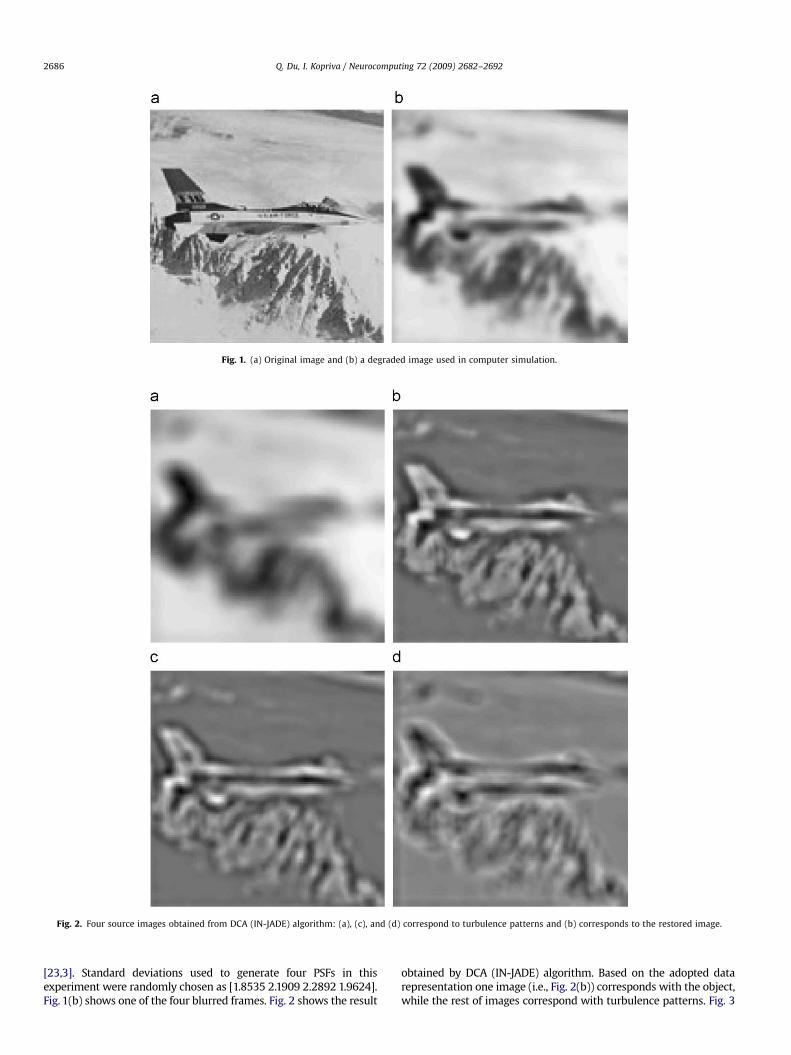
Fig. 1. (a) Original image and (b) a degraded image used in computer simulation.

Fig. 2. Four source images obtained from DCA (IN-JADE) algorithm: (a), (c), and (d) correspond to turbulence patterns and (b) corresponds to the restored image.

Q. Du, I. Kopriva / Neurocomputing 72 (2009) 2682–26922686

[23,3]. Standard deviations used to generate four PSFs in thisexperiment were randomly chosen as [1.8535 2.1909 2.2892 1.9624].Fig. 1(b) shows one of the four blurred frames. Fig. 2 shows the result

obtained by DCA (IN-JADE) algorithm. Based on the adopted datarepresentation one image (i.e., Fig. 2(b)) corresponds with the object,while the rest of images correspond with turbulence patterns. Fig. 3

ARTICLE IN PRESS

Q. Du, I. Kopriva / Neurocomputing 72 (2009) 2682–2692 2687

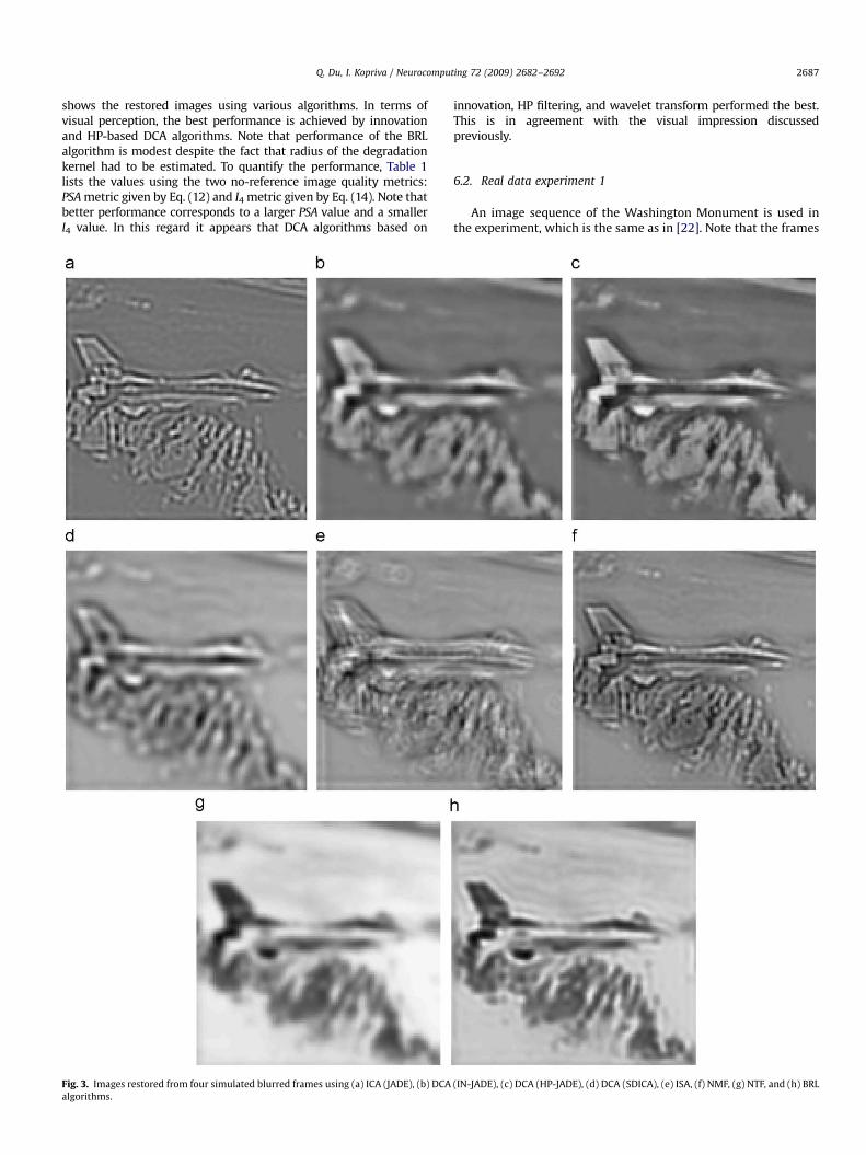
shows the restored images using various algorithms. In terms ofvisual perception, the best performance is achieved by innovationand HP-based DCA algorithms. Note that performance of the BRLalgorithm is modest despite the fact that radius of the degradationkernel had to be estimated. To quantify the performance, Table 1lists the values using the two no-reference image quality metrics:PSA metric given by Eq. (12) and I4 metric given by Eq. (14). Note thatbetter performance corresponds to a larger PSA value and a smallerI4 value. In this regard it appears that DCA algorithms based on

Fig. 3. Images restored from four simulated blurred frames using (a) ICA (JADE), (b) DCA

algorithms.

innovation, HP filtering, and wavelet transform performed the best.This is in agreement with the visual impression discussedpreviously.

6.2. Real data experiment 1

An image sequence of the Washington Monument is used inthe experiment, which is the same as in [22]. Note that the frames

(IN-JADE), (c) DCA (HP-JADE), (d) DCA (SDICA), (e) ISA, (f) NMF, (g) NTF, and (h) BRL

ARTICLE IN PRESS

Table 1No-reference quality assessment for the restored images in computer simulation..

ICA (JADE) DCA (IN-JADE) DCA (HP-JADE) DCA (SDICA) ISA NMF NTF BRL

PSA 3.53 3.90 4.44 3.18 2.87 3.44 2.45 2.66

I4 6.18 2.56 3.66 2.79 4.08 5.21 2.54 3.60

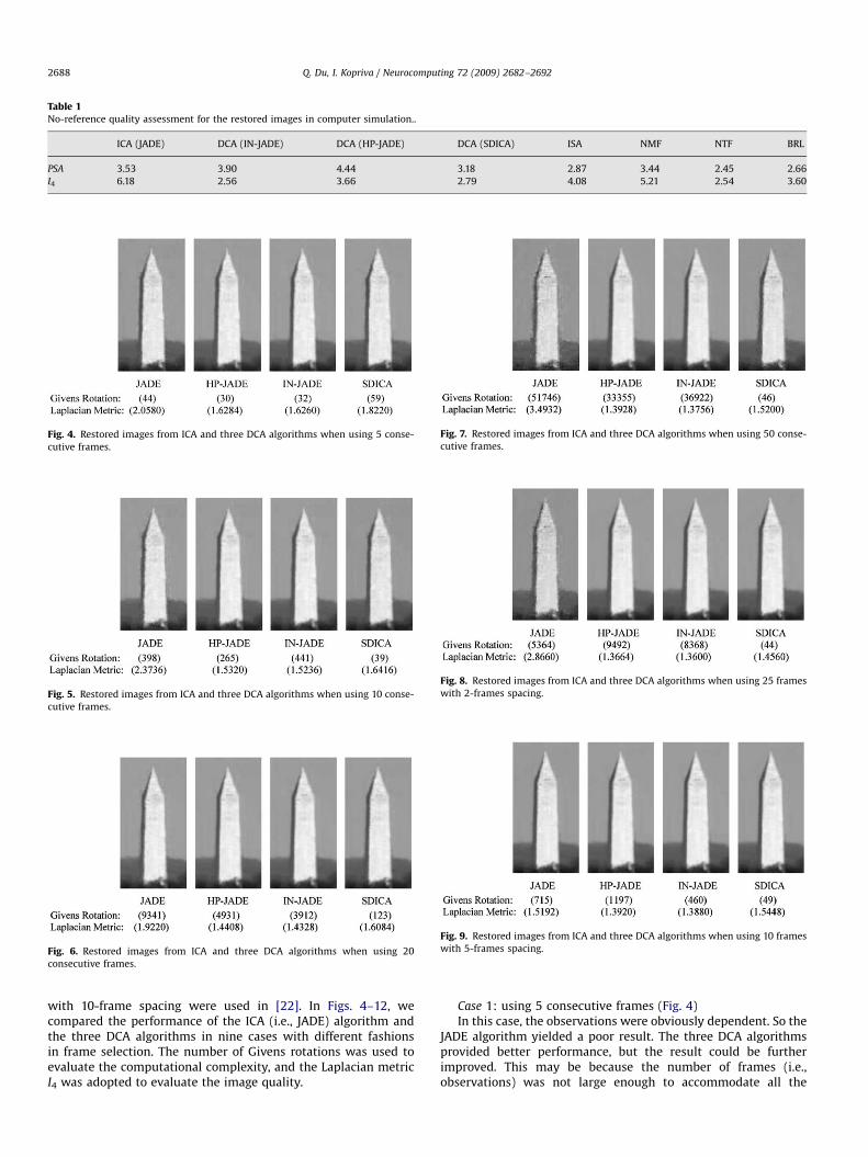
Fig. 4. Restored images from ICA and three DCA algorithms when using 5 conse-

cutive frames.

Fig. 5. Restored images from ICA and three DCA algorithms when using 10 conse-

cutive frames.

Fig. 6. Restored images from ICA and three DCA algorithms when using 20

consecutive frames.

Fig. 7. Restored images from ICA and three DCA algorithms when using 50 conse-

cutive frames.

Fig. 8. Restored images from ICA and three DCA algorithms when using 25 frames

with 2-frames spacing.

Fig. 9. Restored images from ICA and three DCA algorithms when using 10 frames

with 5-frames spacing.

Q. Du, I. Kopriva / Neurocomputing 72 (2009) 2682–26922688

with 10-frame spacing were used in [22]. In Figs. 4–12, wecompared the performance of the ICA (i.e., JADE) algorithm andthe three DCA algorithms in nine cases with different fashionsin frame selection. The number of Givens rotations was used toevaluate the computational complexity, and the Laplacian metricI4 was adopted to evaluate the image quality.

Case 1: using 5 consecutive frames (Fig. 4)In this case, the observations were obviously dependent. So the

JADE algorithm yielded a poor result. The three DCA algorithmsprovided better performance, but the result could be furtherimproved. This may be because the number of frames (i.e.,observations) was not large enough to accommodate all the

ARTICLE IN PRESS

Q. Du, I. Kopriva / Neurocomputing 72 (2009) 2682–2692 2689

sources existing (the number of components that can be extractedis up-bounded by the number of frames).

Case 2: using 10 consecutive frames (Fig. 5)In this case, the observations were strongly dependent. So the

JADE algorithm yielded an even poorer result. Compared to Case 1,the three DCA algorithms provided better performance with thenumber of frames (i.e., observations) being increased.

Case 3: using 20 consecutive frames (Fig. 6)The phenomenon was similar to that in Case 2. The

performance of the JADE algorithm became worse, and theperformance of the three DCA algorithms became better.

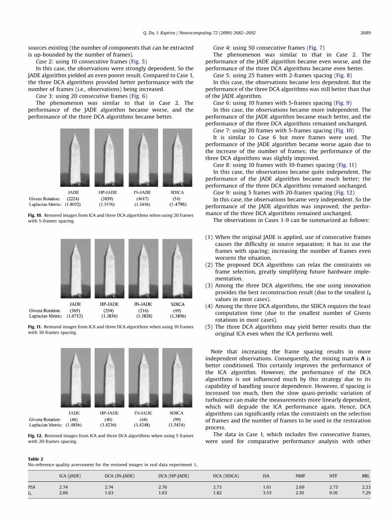
Fig. 10. Restored images from ICA and three DCA algorithms when using 20 frames

with 5-frames spacing.

Fig. 11. Restored images from ICA and three DCA algorithms when using 10 frames

with 10-frames spacing.

Fig. 12. Restored images from ICA and three DCA algorithms when using 5 frames

with 20-frames spacing.

Table 2No-reference quality assessment for the restored images in real data experiment 1..

ICA (JADE) DCA (IN-JADE) DCA (HP-JADE)

PSA 2.74 2.74 2.76

I4 2.06 1.63 1.63

Case 4: using 50 consecutive frames (Fig. 7)The phenomenon was similar to that in Case 2. The

performance of the JADE algorithm became even worse, and theperformance of the three DCA algorithms became even better.

Case 5: using 25 frames with 2-frames spacing (Fig. 8)In this case, the observations became less dependent. But the

performance of the three DCA algorithms was still better than thatof the JADE algorithm.

Case 6: using 10 frames with 5-frames spacing (Fig. 9)In this case, the observations became more independent. The

performance of the JADE algorithm became much better, and theperformance of the three DCA algorithms remained unchanged.

Case 7: using 20 frames with 5-frames spacing (Fig. 10)It is similar to Case 6 but more frames were used. The

performance of the JADE algorithm became worse again due tothe increase of the number of frames; the performance of thethree DCA algorithms was slightly improved.

Case 8: using 10 frames with 10-frames spacing (Fig. 11)In this case, the observations became quite independent. The

performance of the JADE algorithm became much better; theperformance of the three DCA algorithms remained unchanged.

Case 9: using 5 frames with 20-frames spacing (Fig. 12)In this case, the observations became very independent. So the

performance of the JADE algorithm was improved; the perfor-mance of the three DCA algorithms remained unchanged.

The observations in Cases 1-9 can be summarized as follows:

(1)

D

2

1

When the original JADE is applied, use of consecutive framescauses the difficulty in source separation; it has to use theframes with spacing; increasing the number of frames evenworsens the situation.

(2)

The proposed DCA algorithms can relax the constraints onframe selection, greatly simplifying future hardware imple-mentation.

(3)

Among the three DCA algorithms, the one using innovationprovides the best reconstruction result (due to the smallest I4

values in most cases).

(4) Among the three DCA algorithms, the SDICA requires the least

computation time (due to the smallest number of Givensrotations in most cases).

(5)

The three DCA algorithms may yield better results than theoriginal ICA even when the ICA performs well.

Note that increasing the frame spacing results in moreindependent observations. Consequently, the mixing matrix A isbetter conditioned. This certainly improves the performance ofthe ICA algorithm. However, the performance of the DCAalgorithms is not influenced much by this strategy due to itscapability of handling source dependence. However, if spacing isincreased too much, then the slow quasi-periodic variation ofturbulence can make the measurements more linearly dependent,which will degrade the ICA performance again. Hence, DCAalgorithms can significantly relax the constraints on the selectionof frames and the number of frames to be used in the restorationprocess.

The data in Case 1, which includes five consecutive frames,were used for comparative performance analysis with other

CA (SDICA) ISA NMF NTF BRL

.73 1.61 2.69 2.73 2.23

.82 3.53 2.10 9.10 7.29

ARTICLE IN PRESS

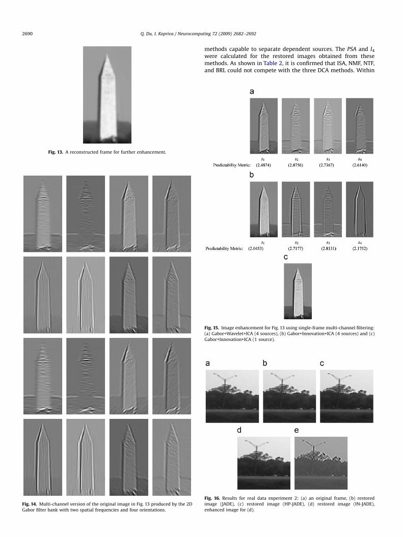
Fig. 13. A reconstructed frame for further enhancement.

Fig. 14. Multi-channel version of the original image in Fig. 13 produced by the 2D

Gabor filter bank with two spatial frequencies and four orientations.

Q. Du, I. Kopriva / Neurocomputing 72 (2009) 2682–26922690

methods capable to separate dependent sources. The PSA and I4

were calculated for the restored images obtained from thesemethods. As shown in Table 2, it is confirmed that ISA, NMF, NTF,and BRL could not compete with the three DCA methods. Within

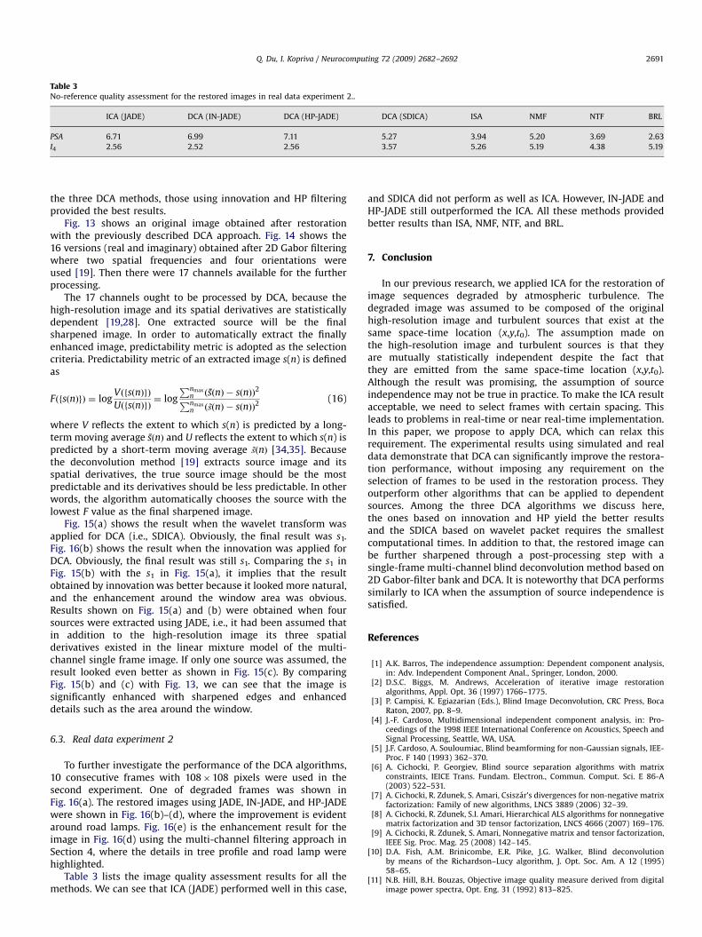
Fig. 15. Image enhancement for Fig. 13 using single-frame multi-channel filtering:

(a) Gabor+Wavelet+ICA (4 sources), (b) Gabor+Innovation+ICA (4 sources) and (c)

Gabor+Innovation+ICA (1 source).

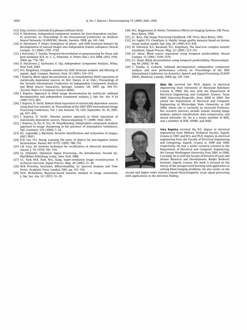
Fig. 16. Results for real data experiment 2: (a) an original frame, (b) restored

image (JADE), (c) restored image (HP-JADE), (d) restored image (IN-JADE),

enhanced image for (d).

ARTICLE IN PRESS

Table 3No-reference quality assessment for the restored images in real data experiment 2..

ICA (JADE) DCA (IN-JADE) DCA (HP-JADE) DCA (SDICA) ISA NMF NTF BRL

PSA 6.71 6.99 7.11 5.27 3.94 5.20 3.69 2.63

I4 2.56 2.52 2.56 3.57 5.26 5.19 4.38 5.19

Q. Du, I. Kopriva / Neurocomputing 72 (2009) 2682–2692 2691

the three DCA methods, those using innovation and HP filteringprovided the best results.

Fig. 13 shows an original image obtained after restorationwith the previously described DCA approach. Fig. 14 shows the16 versions (real and imaginary) obtained after 2D Gabor filteringwhere two spatial frequencies and four orientations wereused [19]. Then there were 17 channels available for the furtherprocessing.

The 17 channels ought to be processed by DCA, because thehigh-resolution image and its spatial derivatives are statisticallydependent [19,28]. One extracted source will be the finalsharpened image. In order to automatically extract the finallyenhanced image, predictability metric is adopted as the selectioncriteria. Predictability metric of an extracted image s(n) is definedas

FðfsðnÞgÞ ¼ logVðfsðnÞgÞ

UðfsðnÞgÞ¼ log

Pnmaxn ðsðnÞ � sðnÞÞ2Pnmaxn ðsðnÞ � sðnÞÞ2

(16)

where V reflects the extent to which s(n) is predicted by a long-term moving average sðnÞ and U reflects the extent to which s(n) ispredicted by a short-term moving average sðnÞ [34,35]. Becausethe deconvolution method [19] extracts source image and itsspatial derivatives, the true source image should be the mostpredictable and its derivatives should be less predictable. In otherwords, the algorithm automatically chooses the source with thelowest F value as the final sharpened image.

Fig. 15(a) shows the result when the wavelet transform wasapplied for DCA (i.e., SDICA). Obviously, the final result was s1.Fig. 16(b) shows the result when the innovation was applied forDCA. Obviously, the final result was still s1. Comparing the s1 inFig. 15(b) with the s1 in Fig. 15(a), it implies that the resultobtained by innovation was better because it looked more natural,and the enhancement around the window area was obvious.Results shown on Fig. 15(a) and (b) were obtained when foursources were extracted using JADE, i.e., it had been assumed thatin addition to the high-resolution image its three spatialderivatives existed in the linear mixture model of the multi-channel single frame image. If only one source was assumed, theresult looked even better as shown in Fig. 15(c). By comparingFig. 15(b) and (c) with Fig. 13, we can see that the image issignificantly enhanced with sharpened edges and enhanceddetails such as the area around the window.

6.3. Real data experiment 2

To further investigate the performance of the DCA algorithms,10 consecutive frames with 108�108 pixels were used in thesecond experiment. One of degraded frames was shown inFig. 16(a). The restored images using JADE, IN-JADE, and HP-JADEwere shown in Fig. 16(b)–(d), where the improvement is evidentaround road lamps. Fig. 16(e) is the enhancement result for theimage in Fig. 16(d) using the multi-channel filtering approach inSection 4, where the details in tree profile and road lamp werehighlighted.

Table 3 lists the image quality assessment results for all themethods. We can see that ICA (JADE) performed well in this case,

and SDICA did not perform as well as ICA. However, IN-JADE andHP-JADE still outperformed the ICA. All these methods providedbetter results than ISA, NMF, NTF, and BRL.

7. Conclusion

In our previous research, we applied ICA for the restoration ofimage sequences degraded by atmospheric turbulence. Thedegraded image was assumed to be composed of the originalhigh-resolution image and turbulent sources that exist at thesame space-time location (x,y,t0). The assumption made onthe high-resolution image and turbulent sources is that theyare mutually statistically independent despite the fact thatthey are emitted from the same space-time location (x,y,t0).Although the result was promising, the assumption of sourceindependence may not be true in practice. To make the ICA resultacceptable, we need to select frames with certain spacing. Thisleads to problems in real-time or near real-time implementation.In this paper, we propose to apply DCA, which can relax thisrequirement. The experimental results using simulated and realdata demonstrate that DCA can significantly improve the restora-tion performance, without imposing any requirement on theselection of frames to be used in the restoration process. Theyoutperform other algorithms that can be applied to dependentsources. Among the three DCA algorithms we discuss here,the ones based on innovation and HP yield the better resultsand the SDICA based on wavelet packet requires the smallestcomputational times. In addition to that, the restored image canbe further sharpened through a post-processing step with asingle-frame multi-channel blind deconvolution method based on2D Gabor-filter bank and DCA. It is noteworthy that DCA performssimilarly to ICA when the assumption of source independence issatisfied.

References

[1] A.K. Barros, The independence assumption: Dependent component analysis,in: Adv. Independent Component Anal., Springer, London, 2000.

[2] D.S.C. Biggs, M. Andrews, Acceleration of iterative image restorationalgorithms, Appl. Opt. 36 (1997) 1766–1775.

[3] P. Campisi, K. Egiazarian (Eds.), Blind Image Deconvolution, CRC Press, BocaRaton, 2007, pp. 8–9.

[4] J.-F. Cardoso, Multidimensional independent component analysis, in: Pro-ceedings of the 1998 IEEE International Conference on Acoustics, Speech andSignal Processing, Seattle, WA, USA.

[5] J.F. Cardoso, A. Souloumiac, Blind beamforming for non-Gaussian signals, IEE-Proc. F 140 (1993) 362–370.

[6] A. Cichocki, P. Georgiev, Blind source separation algorithms with matrixconstraints, IEICE Trans. Fundam. Electron., Commun. Comput. Sci. E 86-A(2003) 522–531.

[7] A. Cichocki, R. Zdunek, S. Amari, Csiszar’s divergences for non-negative matrixfactorization: Family of new algorithms, LNCS 3889 (2006) 32–39.

[8] A. Cichocki, R. Zdunek, S.I. Amari, Hierarchical ALS algorithms for nonnegativematrix factorization and 3D tensor factorization, LNCS 4666 (2007) 169–176.

[9] A. Cichocki, R. Zdunek, S. Amari, Nonnegative matrix and tensor factorization,IEEE Sig. Proc. Mag. 25 (2008) 142–145.

[10] D.A. Fish, A.M. Brinicombe, E.R. Pike, J.G. Walker, Blind deconvolutionby means of the Richardson–Lucy algorithm, J. Opt. Soc. Am. A 12 (1995)58–65.

[11] N.B. Hill, B.H. Bouzas, Objective image quality measure derived from digitalimage power spectra, Opt. Eng. 31 (1992) 813–825.

ARTICLE IN PRESS

Q. Du, I. Kopriva / Neurocomputing 72 (2009) 2682–26922692

[12] http://www.cs.helsinki.fi/u/phoyer/software.html.[13] A. Hyvarinen, Independent component analysis for time-dependent stochas-

tic processes, in: Proceedings of the International Conference on ArtificialNeural Networks (ICANN’98), Skovde, Sweden, 1998, pp. 541–546.

[14] A. Hyvarinen, P. Hoyer, Emergence of phase- and shift-invariant features bydecomposition of natural images into independent feature subspaces, NeuralComput. 12 (2000) 1705–1720.

[15] J. Karvanen, T. Tanaka, Temporal decorrelation as preprocessing for linear andpost-nonlinear ICA, in: C. G. Puntonet, A. Prieto (Eds.), ICA 2004, LNCS 3195,2004, pp. 774–781.

[16] A. Hyvarinen, J. Karhunen, E. Oja, Independent Component Analysis, Wiley,New York, 2001.

[17] N.G. Kingsbury, Complex wavelets for shift invariant analysis and filtering ofsignals, Appl. Comput. Harmon. Anal. 10 (2001) 234–253.

[18] I. Kopriva, Blind signal deconvolution as an instantaneous blind separation ofstatistically dependent sources, in: M.E. Davies, et al. (Eds.), Proceedings ofthe Seventh International Conference on Independent Component Analysisand Blind Source Separation, Springer, London, UK, 2007, pp. 504–511(Lecture Notes in Computer Science 4666).

[19] I. Kopriva, Approach to blind image deconvolution by multiscale subbanddecomposition and independent component analysis, J. Opt. Soc. Am. A 24(2007) 973–983.

[20] I. Kopriva, D. Sersic, Robust blind separation of statistically dependent sourcesusing dual tree wavelets, in: Proceedings of the 2007 IEEE International ImageProcessing Conference, Vol. I, San Antonio, TX, USA, September 16–19, 2007,pp. 433–436.

[21] I. Kopriva, D. Sersic, Wavelet packets approach to blind separation ofstatistically dependent sources, Neurocomputing 71 (2008) 1642–1655.

[22] I. Kopriva, Q. Du, H. Szu, W. Wasylkiwskyj, Independent component analysisapproach to image sharpening in the presence of atmospheric turbulence,Opt. Commun. 233 (2004) 7–14.

[23] R.L. Lagendijk, J. Biemond, Iterative identification and restoration of images,KAP (1991).

[24] D.D. Lee, H.S. Seung, Learning the parts of objects by non-negative matrixfactorization, Nature 401–6755 (1999) 788–791.

[25] L.B. Lucy, An iterative technique for rectification of observed distribution,Astron. J. 79 (1974) 745–754.

[26] S.J. Orfanidis, Optimum Signal Processing—An Introduction, Second ed.,MacMillan Publishing Comp., New York, 1988.

[27] S.C. Park, M.K. Park, M.G. Kang, Super-resolution image reconstruction: Atechnical overview, Signal Process. Mag. 20 (2003) 21–36.

[28] M.B. Priestley, Stochastic differentiability, in: Spectral Analysis and TimeSeries, Academic Press, London, 1981, pp. 153–154.

[29] W.H. Richardson, Bayesian-based iterative method of image restoration,J. Opt. Soc. Am. 62 (1972) 55–59.

[30] M.C. Roggemann, B. Welsh, Turbulence Effects on Imaging Systems, CRC Press,Boca Raton, 1996.

[31] J.C. Russ, The Image Processing Handbook, CRC Press, Boca Raton, 1992.[32] J.A. Saghri, P.S. Cheatham, A. Habibi, Image quality measure based on human

visual system model, Opt. Eng. 28 (1989) 813–818.[33] W. Selesnick, R.G. Baraniuk, N.G. Kingsbury, The dual-tree complex wavelet

transform, Signal Process. Mag. 22 (2005) 123–151.[34] J.V. Stone, Blind source separation using temporal predictability, Neural

Comput. 13 (2001) 1559–1574.[35] J.V. Stone, Blind deconvolution using temporal predictability, Neurocomput-

ing 49 (2002) 79–86.[36] T. Tanaka, A. Cichocki, Subband decomposition independent component

analysis and new performance criteria, in: Proceedings of the IEEEInternational Conference on Acoustics, Speech and Signal Processing (ICASSP2004), Montreal, Canada, 2004, pp. 541–544.

Qian Du received her Ph.D. degree in electricalengineering from University of Maryland BaltimoreCounty in 2000. She was with the Department ofElectrical Engineering and Computer Science, TexasA&M University-Kingsville, from 2000 to 2004. Shejoined the Department of Electrical and ComputerEngineering at Mississippi State University in Fall2004, where she is currently an Associate Professor.Her research interests include remote sensing imageanalysis, pattern classification, data compression, andneural networks. Dr. Du is a senior member of IEEE,and a member of SPIE, ASPRS, and ASEE.

Ivica Kopriva received the B.S. degree in electricalengineering from Military Technical Faculty, Zagreb,Croatia in 1987, and M.S. and Ph.D. degrees in electricalengineering from the Faculty of Electrical Engineeringand Computing, Zagreb, Croatia in 1990 and 1998,respectively. He was a senior research scientist in theDepartment of Electrical and Computer Engineering,the George Washington University from 2001 to 2006.Currently, he is with the faculty of Division of Laser andAtomic Research and Development, Rudjer BoskovicInstitute, Zagreb, Croatia. His work is focused on thetheory of the unsupervised learning with application in

solving blind imaging problems. He also works on the

second and higher order statistics-based electromagnetic array signal processingwith applications in the direction finding.