
DEPARTMENT OF MATHEMATICSijsrme.rdmodernresearch.com/wp-content/uploads/2016/04/TP002.pdfnumerical...
90
NUMERICAL METHODS FOR SOLVING DEs WITH MATLAB This project work is submitted to ST.JOSEPH’S COLLEGE (AUTONOMOUS) In partial fulfillment of the requirements of the degree of MASTER OF PHILOSOPHY IN MATHEMATICS by SAHAYA JERNITH.S (Reg.No:12MMA115) Under the guidance of Dr. S. RUBANRAJ, M.Sc., B.Ed., M.Phil., PGDCSA., Ph.D., DEPARTMENT OF MATHEMATICS ST.JOSEPH’S COLLEGE (AUTONOMOUS) Nationally Re-Accredited (3 rd cycle ) With A Grade College With Potential For Excellence Trichirappalli – 620 002 August – 2013.
Transcript of DEPARTMENT OF MATHEMATICSijsrme.rdmodernresearch.com/wp-content/uploads/2016/04/TP002.pdfnumerical...

NUMERICAL METHODS FOR SOLVING DEs
WITH MATLAB
This project work is submitted to
ST.JOSEPH’S COLLEGE (AUTONOMOUS)
In partial fulfillment of the requirements of the degree of
MASTER OF PHILOSOPHY IN MATHEMATICS
by
SAHAYA JERNITH.S
(Reg.No:12MMA115)
Under the guidance of
Dr. S. RUBANRAJ, M.Sc., B.Ed., M.Phil., PGDCSA., Ph.D.,
DEPARTMENT OF MATHEMATICS
ST.JOSEPH’S COLLEGE (AUTONOMOUS)
Nationally Re-Accredited (3rd cycle) With A Grade
College With Potential For Excellence
Trichirappalli – 620 002
August – 2013.

Certificate
This is to certify that the project entitled “NUMERICAL METHODS
FOR SOLVING DEs WITH MATLAB” submitted to St.Joseph’s
College (Autonomous), affiliated by Bharathidasan University, Trichy – 24,
by SAHAYA JERNITH.S (12MMA115) for the partial fulfilment of
award of the degree of Master of Philosophy in Mathematics is a record
of bonafide work carried out by her under my guidance and supervision in
the year 2012 - 2013.
HEAD OF THE DEPARTMENT RESEARCH ADVISOR
Dr.S.RUBANRAJ Dr.S.RUBANRAJ
Department of Mathematics Department of Mathematics
St. Joseph’s College (Autonomous) St. Joseph’s College (Autonomous)
Tiruchirappalli – 620 002. Tiruchirappalli – 620 002.
Viva-Voce examination conducted on · · · · · · · · · · · · · · · · · · · · · · · · at St.Joseph’s
College (Autonomous) Tiruchirappalli – 620 002.
Place: Tiruchirappalli EXTERNAL EXAMINER
Date :
Acknowledgement
I would like to express my grateful thanks to Almighty God for giving me
the strength and the wisdom for completing this project.
I would like to convey my heartfelt and sincere thanks to my guide and
Head of the Department of Mathematics Dr. S. RUBANRAJ, M.Sc., B.Ed.,
M.Phil., PGDCSA., Ph.D., Department of Mathematics, St. Joseph’s Col-
lege (Autonomous), Tiruchirappalli-620002, for his unfailing enthusiasm and
endless encouragement in my endeavours. It is not an exaggeration to state
that he is a great source of inspiration and illumination to me.
I am privileged to express my gratitude to Rev.Dr.A.ALBERT MUTHU-
MALAI, SJ, Former Principal, St.Joseph’s College (Autonomous), Trichy
and Rev.Dr.F.ANDREW, SJ, Principal, St.Joseph’s College (Autonomous),
Trichy, for having given me wonderful opportunity to study in this presti-
gious institution.
Last but not the least, I would like to express my gratitude to all mem-
bers, my relations and my friends for their precious support through their
prayers for the successful completion of this dissertation. I whole heartedly
thank my beloved parents for being a great source of inspiration, a role model
and of course, for their invaluable love.
SAHAYA JERNITH.S
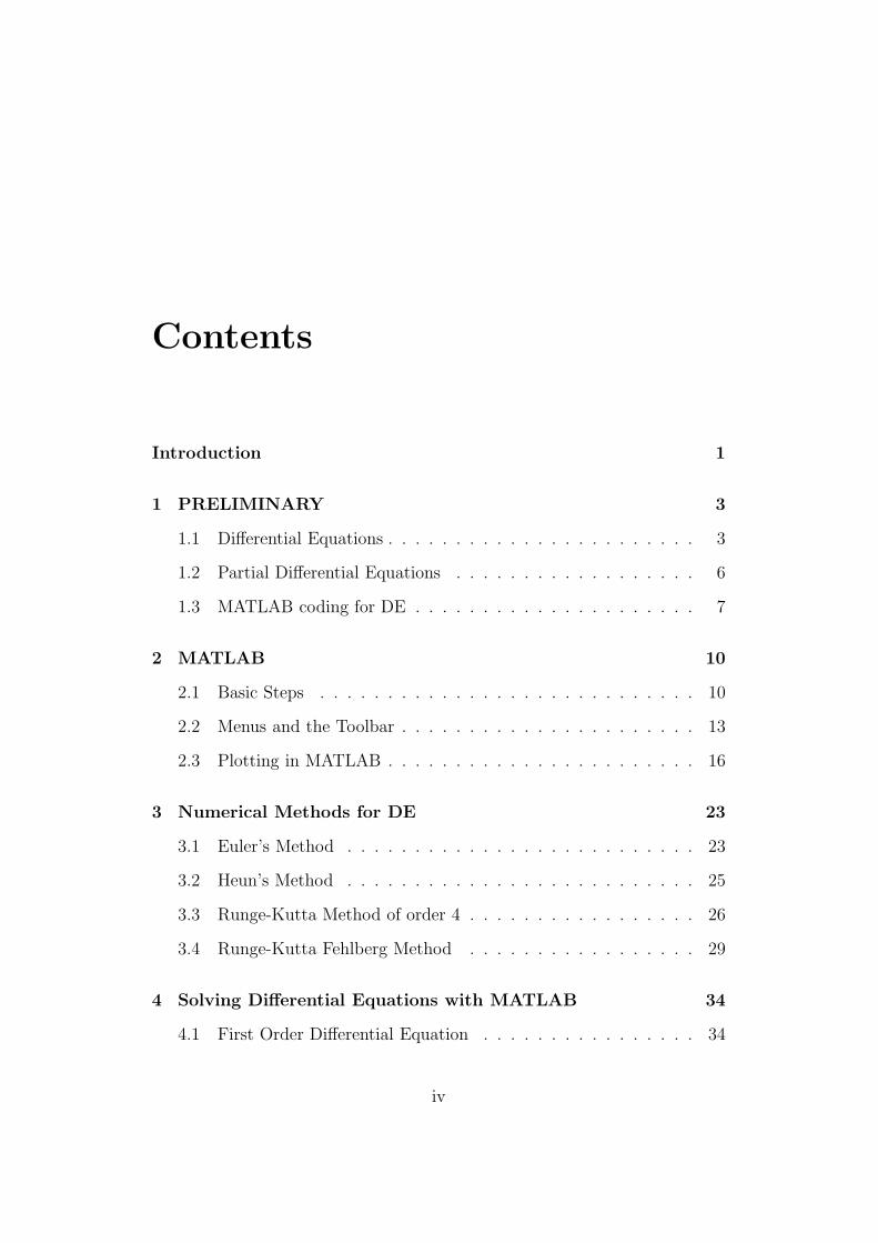
Contents
Introduction 1
1 PRELIMINARY 3
1.1 Differential Equations . . . . . . . . . . . . . . . . . . . . . . . 3
1.2 Partial Differential Equations . . . . . . . . . . . . . . . . . . 6
1.3 MATLAB coding for DE . . . . . . . . . . . . . . . . . . . . . 7
2 MATLAB 10
2.1 Basic Steps . . . . . . . . . . . . . . . . . . . . . . . . . . . . 10
2.2 Menus and the Toolbar . . . . . . . . . . . . . . . . . . . . . . 13
2.3 Plotting in MATLAB . . . . . . . . . . . . . . . . . . . . . . . 16
3 Numerical Methods for DE 23
3.1 Euler’s Method . . . . . . . . . . . . . . . . . . . . . . . . . . 23
3.2 Heun’s Method . . . . . . . . . . . . . . . . . . . . . . . . . . 25
3.3 Runge-Kutta Method of order 4 . . . . . . . . . . . . . . . . . 26
3.4 Runge-Kutta Fehlberg Method . . . . . . . . . . . . . . . . . 29
4 Solving Differential Equations with MATLAB 34
4.1 First Order Differential Equation . . . . . . . . . . . . . . . . 34
iv

CONTENTS v
4.2 Second Order Differential Equations . . . . . . . . . . . . . . . 36
4.3 System of Differential Equations . . . . . . . . . . . . . . . . . 37
4.4 Runge-Kutta methods in MATLAB . . . . . . . . . . . . . . . 41
4.5 Euler Methods . . . . . . . . . . . . . . . . . . . . . . . . . . 45
5 Comparison of numerical approximations 51
5.1 Comparison for a first order ODE . . . . . . . . . . . . . . . . 51
5.2 Comparison for a system of ODEs . . . . . . . . . . . . . . . . 64
6 Solving Partial Differential Equations with MATLAB 71
6.1 Poisson’s Equation on a Unit Disc . . . . . . . . . . . . . . . . 74
6.2 Helmholtz’s Equation on a Unit Disk with a Square Hole . . . 78
6.3 Solve for Complex Amplitude . . . . . . . . . . . . . . . . . . 79
6.4 Animate Solution to Wave Equation . . . . . . . . . . . . . . 80
Conclusion 82
Bibliography 83
v

List of Figures
1.1 Van Der Pol Equation . . . . . . . . . . . . . . . . . . . . . . 9
2.1 Graph of cosine function . . . . . . . . . . . . . . . . . . . . . 17
2.2 Graph of cosine function from −π to π . . . . . . . . . . . . . 18
2.3 Graph of cosine function in dotted line . . . . . . . . . . . . . 19
2.4 Graph of cosine and sine functions . . . . . . . . . . . . . . . 20
2.5 Graph of meshgrid . . . . . . . . . . . . . . . . . . . . . . . . 21
4.1 Solution of the equation y′ = xy, y(1) = 1 . . . . . . . . . . . 35
4.2 Solution of the DE y + 8y + 2y = cos(x) y(0) = 0 y′(0) = 1 37
4.3 Solutions of x′ = x+ 2y − z, y′ = x+ z, z′ = 4x− 4y + 5z . . 39
4.4 Graph of Lorenz equations . . . . . . . . . . . . . . . . . . . . 40
4.5 Graph of Components for the Lorenz Equations . . . . . . . . 41
4.6 Graph of epidemiology growth of market share . . . . . . . . . 42
4.7 Graph of x(t) vs t for the ODE . . . . . . . . . . . . . . . . . 43
4.8 Graph of y vs t for the ODE . . . . . . . . . . . . . . . . . . . 44
4.9 Graph of y vs x for the ODE . . . . . . . . . . . . . . . . . . . 44
4.10 Graph of the solution by Euler’s methods and the analytical
solution . . . . . . . . . . . . . . . . . . . . . . . . . . . . . . 48
vi
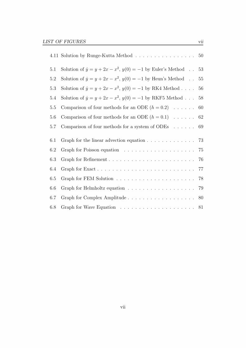
LIST OF FIGURES vii
4.11 Solution by Runge-Kutta Method . . . . . . . . . . . . . . . . 50
5.1 Solution of y = y + 2x− x2, y(0) = −1 by Euler’s Method . . 53
5.2 Solution of y = y + 2x− x2, y(0) = −1 by Heun’s Method . . 55
5.3 Solution of y = y + 2x− x2, y(0) = −1 by RK4 Method . . . . 56
5.4 Solution of y = y + 2x− x2, y(0) = −1 by RKF5 Method . . . 58
5.5 Comparison of four methods for an ODE (h = 0.2) . . . . . . 60
5.6 Comparison of four methods for an ODE (h = 0.1) . . . . . . 62
5.7 Comparison of four methods for a system of ODEs . . . . . . 69
6.1 Graph for the linear advection equation . . . . . . . . . . . . . 73
6.2 Graph for Poisson equation . . . . . . . . . . . . . . . . . . . 75
6.3 Graph for Refinement . . . . . . . . . . . . . . . . . . . . . . . 76
6.4 Graph for Exact . . . . . . . . . . . . . . . . . . . . . . . . . . 77
6.5 Graph for FEM Solution . . . . . . . . . . . . . . . . . . . . . 78
6.6 Graph for Helmholtz equation . . . . . . . . . . . . . . . . . . 79
6.7 Graph for Complex Amplitude . . . . . . . . . . . . . . . . . . 80
6.8 Graph for Wave Equation . . . . . . . . . . . . . . . . . . . . 81
vii

Introduction
Numerical methods are commonly used for solving mathematical problems
that are formulated in science and engineering where it is difficult or even
impossible to obtain exact solutions. Only a limited number of differential
equations can be solved analytically. Numerical methods, on the other hand,
can give an approximate solution to (almost) any equation. An ordinary dif-
ferential equation (ODE) is an equation that contains an independent vari-
able, a dependent variable, and derivatives of the dependent variable. Literal
implementation of this procedure results in Euler’s method, which is, how-
ever, not recommended for any practical use. There are other methods more
sophisticated than Euler’s. Among them, there are four types of practical
numerical methods for solving problems of ODEs. They are (i) Runge-Kutta
Methods, (ii) Heun’s Method, (iii) RK4 Method, and (iv)RKF5 Method.
MATLAB is an integrated technical computing environment that com-
bines numeric computation, advanced graphics and visualization and a high-
level programming language. MATLAB was founded by Jack Little Cleve
Moler and Steve Bangert in 1984. Color graphics makes it possible to display
curves, surfaces, and solids in two and three dimensions in a way that it is
both more effective and more engaging. The easy syntax of MATLAB makes
it possible for users to get comfortable results quickly. MATLAB graphics
1

Introduction 2
are excellent and easy to use. It is easy to program in MATLAB, making
it possible to do numerical calculations using simple steps. We can also use
the symbolic capability of MATLAB to get analytical solutions. MATLAB
is becoming the most popular software package in Mathematics.
• In first chapter, we study the preliminaries needed to use MATLAB to
solve problems in ODEs. We see basic definitions based on Differential
Equation and Partial Differential Equation. We introduce MATLAB
plotting to simulate the solution of Differential Equation problems.
• In second chapter, we review the software package MATLAB for high-
performance numerical computation and visualization which provides
an interactive environment with hundreds of built-in-functions for tech-
nical computation, graphics and animation.
• In third chapter, we discuss the various Numerical Methods available
for solving DEs and they are (1) Euler’s method, (2) Heun’s method,
(3) RK4 method and (4) RKF5 method.
• In fourth chapter, we study the MATLAB programs for Solving Dif-
ferential Equations. Also we study Euler methods and Runge-Kutta
methods in MATLAB.
• In fifth chapter, we compare various methods and their approximation
for 1st order differential equation and a system of ODEs. We also test
the problem with the above methods.
• In sixth chapter, we attempt to simulate the solution of few partial
differential equations using MATLAB.
2
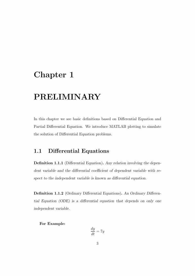
Chapter 1
PRELIMINARY
In this chapter we see basic definitions based on Differential Equation and
Partial Differential Equation. We introduce MATLAB plotting to simulate
the solution of Differential Equation problems.
1.1 Differential Equations
Definition 1.1.1 (Differential Equation). Any relation involving the depen-
dent variable and the differential coefficient of dependent variable with re-
spect to the independent variable is known as differential equation.
Definition 1.1.2 (Ordinary Differential Equations). An Ordinary Differen-
tial Equation (ODE) is a differential equation that depends on only one
independent variable.
For Example:
dy
dt= 7y
3
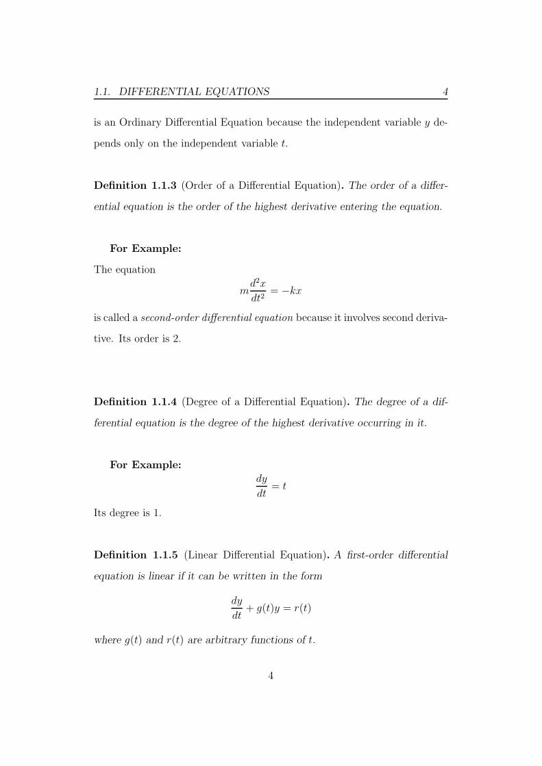
1.1. DIFFERENTIAL EQUATIONS 4
is an Ordinary Differential Equation because the independent variable y de-
pends only on the independent variable t.
Definition 1.1.3 (Order of a Differential Equation). The order of a differ-
ential equation is the order of the highest derivative entering the equation.
For Example:
The equation
md2x
dt2= −kx
is called a second-order differential equation because it involves second deriva-
tive. Its order is 2.
Definition 1.1.4 (Degree of a Differential Equation). The degree of a dif-
ferential equation is the degree of the highest derivative occurring in it.
For Example:
dy
dt= t
Its degree is 1.
Definition 1.1.5 (Linear Differential Equation). A first-order differential
equation is linear if it can be written in the form
dy
dt+ g(t)y = r(t)
where g(t) and r(t) are arbitrary functions of t.
4

1.1. DIFFERENTIAL EQUATIONS 5
For Example:
dy
dt+ 4y = cos t
is a first-order linear differential equation where g(t) = 4 and r(t) = cos t.
Definition 1.1.6 (Homogeneous Differential Equation). A linear first-order
differential equation is homogeneous if its right hand side is zero , that is
r(t) = 0. ∴dy
dt+ g(t)y = 0.
For Example:
dy
dt+ ky(t) = 0
, where k is a constant, is homogeneous.
Definition 1.1.7 (Non-homogeneous Differential Equation). A linear first-
order differential equation is non-homogeneous if its right-hand side is non-
zero, that is, r(t) 6= 0.
dy
dt+ g(t)y = r(t)
For Example:
∴
dy
dt+ 2y = sin 2t
is non-homogeneous.
Definition 1.1.8 (Non-linear Differential Equation). It is a differential equa-
tion whose right hand side is not a linear function of the dependent variable.
5
1.2. PARTIAL DIFFERENTIAL EQUATIONS 6
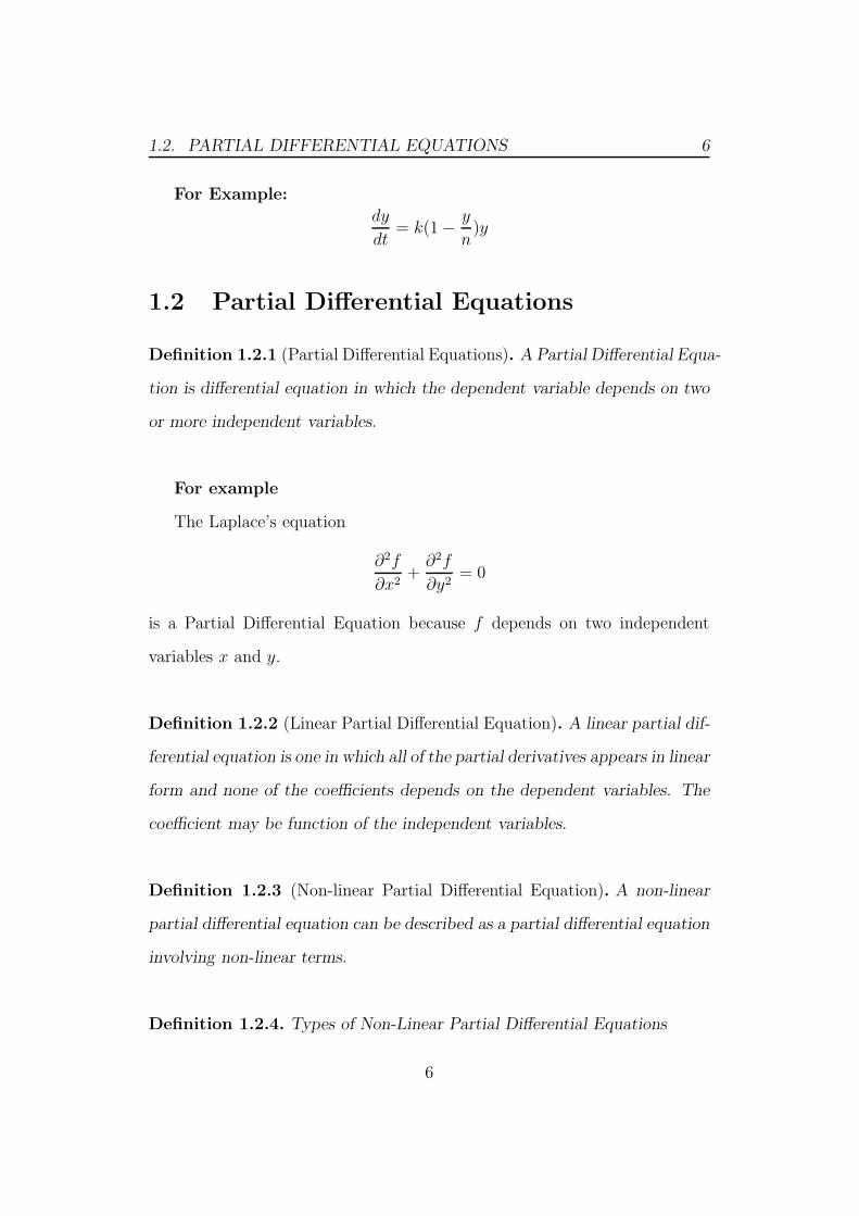
For Example:
dy
dt= k(1− y
n)y
1.2 Partial Differential Equations
Definition 1.2.1 (Partial Differential Equations). A Partial Differential Equa-
tion is differential equation in which the dependent variable depends on two
or more independent variables.
For example
The Laplace’s equation
∂2f
∂x2+
∂2f
∂y2= 0
is a Partial Differential Equation because f depends on two independent
variables x and y.
Definition 1.2.2 (Linear Partial Differential Equation). A linear partial dif-
ferential equation is one in which all of the partial derivatives appears in linear
form and none of the coefficients depends on the dependent variables. The
coefficient may be function of the independent variables.
Definition 1.2.3 (Non-linear Partial Differential Equation). A non-linear
partial differential equation can be described as a partial differential equation
involving non-linear terms.
Definition 1.2.4. Types of Non-Linear Partial Differential Equations
6
1.3. MATLAB CODING FOR DE 7
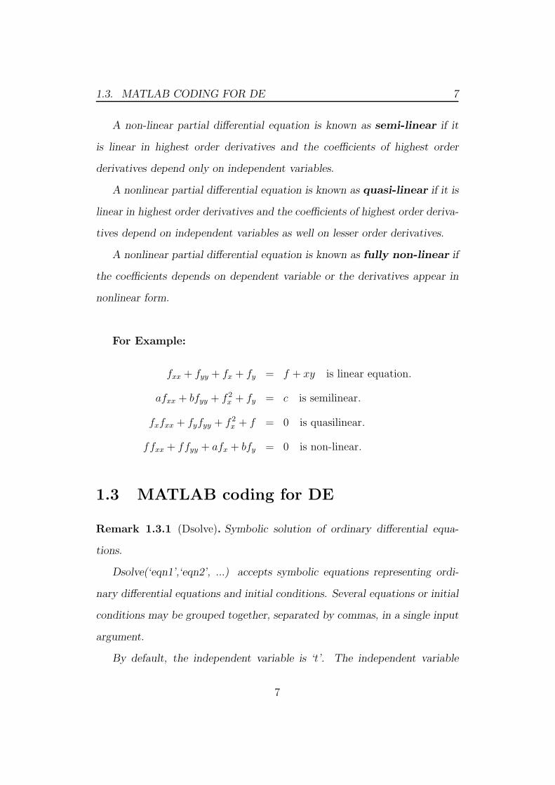
A non-linear partial differential equation is known as semi-linear if it
is linear in highest order derivatives and the coefficients of highest order
derivatives depend only on independent variables.
A nonlinear partial differential equation is known as quasi-linear if it is
linear in highest order derivatives and the coefficients of highest order deriva-
tives depend on independent variables as well on lesser order derivatives.
A nonlinear partial differential equation is known as fully non-linear if
the coefficients depends on dependent variable or the derivatives appear in
nonlinear form.
For Example:
fxx + fyy + fx + fy = f + xy is linear equation.
afxx + bfyy + f 2x + fy = c is semilinear.
fxfxx + fyfyy + f 2x + f = 0 is quasilinear.
ffxx + ffyy + afx + bfy = 0 is non-linear.
1.3 MATLAB coding for DE
Remark 1.3.1 (Dsolve). Symbolic solution of ordinary differential equa-
tions.
Dsolve(‘eqn1’,‘eqn2’, ...) accepts symbolic equations representing ordi-
nary differential equations and initial conditions. Several equations or initial
conditions may be grouped together, separated by commas, in a single input
argument.
By default, the independent variable is ‘t’. The independent variable
7
1.3. MATLAB CODING FOR DE 8
may be changed from ‘t’ to some other symbolic variable by including that
variable as the last input argument.
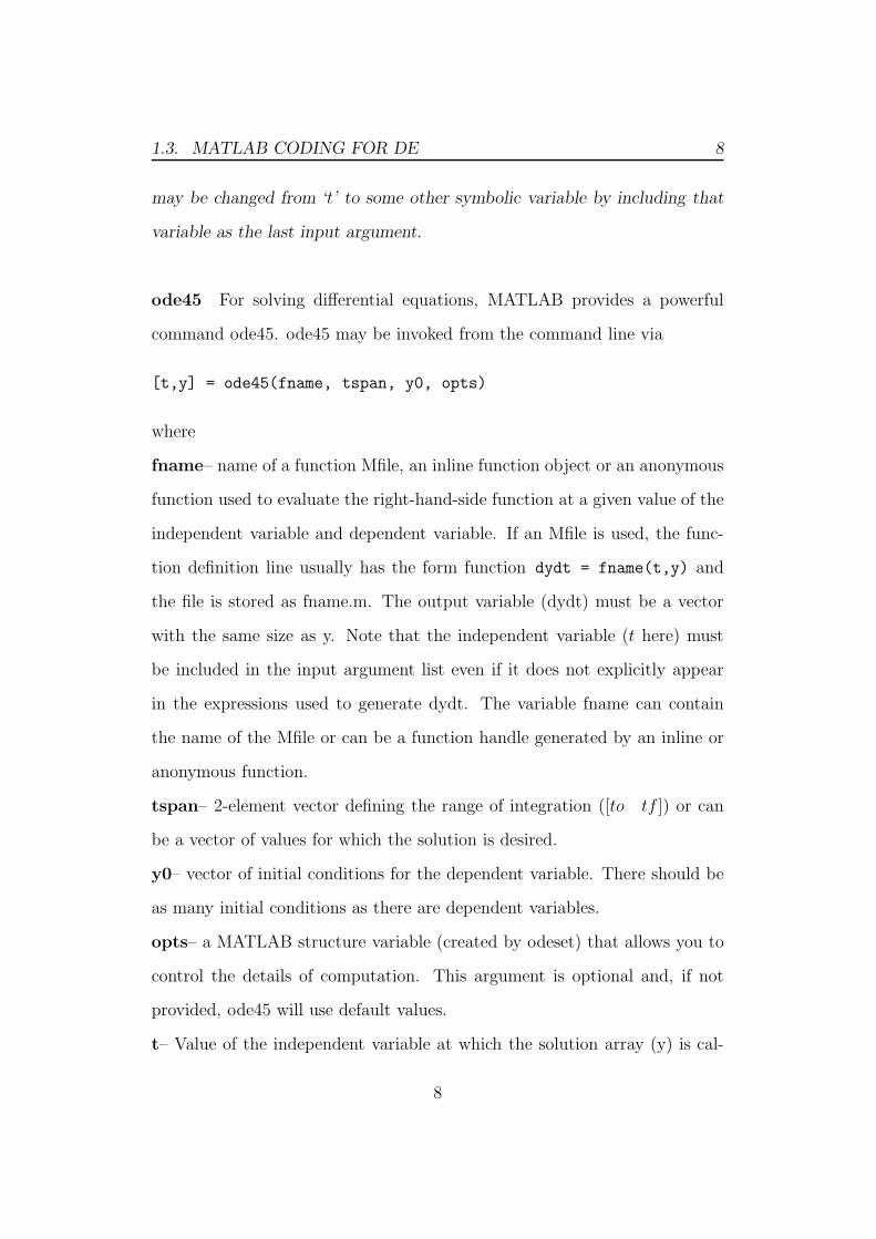
ode45 For solving differential equations, MATLAB provides a powerful
command ode45. ode45 may be invoked from the command line via
[t,y] = ode45(fname, tspan, y0, opts)
where
fname– name of a function Mfile, an inline function object or an anonymous
function used to evaluate the right-hand-side function at a given value of the
independent variable and dependent variable. If an Mfile is used, the func-
tion definition line usually has the form function dydt = fname(t,y) and
the file is stored as fname.m. The output variable (dydt) must be a vector
with the same size as y. Note that the independent variable (t here) must
be included in the input argument list even if it does not explicitly appear
in the expressions used to generate dydt. The variable fname can contain
the name of the Mfile or can be a function handle generated by an inline or
anonymous function.
tspan– 2-element vector defining the range of integration ([to tf ]) or can
be a vector of values for which the solution is desired.
y0– vector of initial conditions for the dependent variable. There should be
as many initial conditions as there are dependent variables.
opts– a MATLAB structure variable (created by odeset) that allows you to
control the details of computation. This argument is optional and, if not
provided, ode45 will use default values.
t– Value of the independent variable at which the solution array (y) is cal-
8

1.3. MATLAB CODING FOR DE 9
culated. Note that by default this will not be a uniformly distributed set of
values.
y– Values of the solution to the problem (array). Each column of y is a
different dependent variable. The size of the array is length(t)-by-length(y0)
Example for ode45
Consider the second order differential equation known as Van-der-pol
equation x + (x2 − 1)x + x = 0. Rewrite this as a system of coupled first
order differential equations: x1 = x1(1− x22)− x2 and x2 = x1. To simulate
the differential equation defined in vdpol over the interval 0 ≤ t ≤ 20, we
invoke ode23.
function xdot = vdpol(t,x)
xdot = [x(1).*(1-x(2).^2)-x(2); x(1)]
t0 = 0; tf = 20;
x0 = [0 0.25]’;
[t,x] = ode23(‘vdpol’,t0,tf,x0);
plot(t,x)
Figure 1.1: Van Der Pol Equation
0 5 10 15 20−3
−2
−1
0
1
2
3
9
Chapter 2
MATLAB
MATLAB is a software package for high-performance numerical computation
and visualization. It provides an interactive environment with hundreds of
built-in-functions for technical computation graphics and animation. It also
provides easy extensibility with its own high-level programming language.
The name MATLAB stands for MATrix LABoratory.
MATLAB is primarily a numerical computation package, although with
the symbolic MATH toolbox it can so symbolic algebra. MATLAB was pri-
marily designed to do numerical calculations. MATLAB is often much faster
at these calculations. MATLAB deals numerical computation, especially
those use vectors and matrices.
2.1 Basic Steps
The Command Line
First Steps:
10

2.1. BASIC STEPS 11
When we invoke MATLAB to begin a session, we see the prompt
>>
We can give instructions for an operation, or request information,
following this prompt, on the command line.
We can do simple arithmetic operations like (2 + 3.52 − 4.7)/12 on the
command line.
>> (2 + 3.5∧2− 4 ∗ 7)/12
ans =
−1.1458
We can also do this calculation by assigning variable names to the quan-
tities. If we do not wish to see the intermediate results, we can suppress the
numerical output by putting a semicolon at the end of the line. Then the
sequence of commands and output looks like this:
>> x = 2 + 3.5∧2;
>> y = 4 ∗ 7;
>> z = (x− y)/12;
>> z
z =
− 1.1458
Error Message
11

2.1. BASIC STEPS 12
If we enter an expression incorrectly, MATLAB will return an error mes-
sage, which always locates the error. For example, in the following, we left
out the ∗ in 3 ∗ x
>> x = 4;
>> 3x
???3
|
Missing operator, comma, or semicolon.
Making Corrections
To make corrections, we can, of course, retype the expression. But if
the expression is lengthy, we may make more mistakes by typing a second
time. Unfortunately we cannot move the cursor to the line we wish to repair.
Instead we can press the up-arrow key until we reach the desired line and
then the left- and right-arrows until we reach the offending characters. Type
in the correction and enter return.
Exiting
To leave MATLAB session, enter quit. If MATLAB gets hung up in
calculation or is taking a long time, and you want to stop the calculation,
without exiting MATLAB, enter Ctrl+C.
Help
To get information on a particular command or operation, simply enter
help command name. For example, to get information on how to use the
12

2.2. MENUS AND THE TOOLBAR 13
plotting commands, enter help plot.
2.2 Menus and the Toolbar
The Desktop manages the Command window and other MATLAB tools.
Across the top of the Desktop are a row of menu names, and a row of icons
called the toolbar. To the right of the toolbar is a box showing the current
directory, where MATLAB looks for files.
Other windows appear in a MATLAB session, depending on the work to
do. For example, a graphics window containing a plot appears to use the
plotting functions; an editor window, called the Editor/Debugger, appears
for use in creating program files.
Each window type has its own menu bar, with one or more menus, at the
top. Thus the menu bar will change as you change windows. To activate, or
select, a menu, click on it. Each menu has several items. Click on an item to
select it. Keep in mind that menus are context-sensitive. Thus their contents
change, depending on which features you are currently using.
The Desktop Menus
Most of the interaction will be in the Command window. When the Com-
mand window is active, the default MATLAB has six menus: File, Edit,
Debug, Desktop, Window, and Help. These menus change depending
on what window is active. Every item on a menu can be selected with the
menu open either by clicking on the item or by typing its underlined letter.
The three most useful menus are the File, Edit, and Help menus.
The File menu in MATLAB contains the following items, which perform
the indicated actions when we select them.
13

2.2. MENUS AND THE TOOLBAR 14
The File Menu
New:Opens a dialog box that allow to create a new program file, called an
M-file, using a text editor called the Editor/Debugger, or a new Figure or
Model file.
Open: Opens a dialog box that allows you to select a file for editing.
Close Command Window: Closes the Command window.
Import Data: Starts the Import Wizard which enables you to import data
easily.
Save Workspace As: Opens a dialog box that enables you to save a file.
Set Path: Opens a dialog box that enables you to set the MATLAB search
path.
Preferences: Opens a dialog box that enables you to set preferences for
such items as fonts, colors, tab spacing, and so forth.
Page Setup: Opens a dialog box that enables you to format printed output.
Print: Opens a dialog box that enables you to print all of the Command
window.
Print Selection: Opens a dialog box that enables you to print selected
portions of the Command window.
File List: Contains a list of previously used files, in order of most recently
used.
Exit MATLAB: Closes MATLAB.
TheEdit menu contains the following items.
The Edit Menu
Undo: Reverses the previous editing operation.
Redo: Reverses the previous Undo operation.
14
2.2. MENUS AND THE TOOLBAR 15
Cut: Removes the selected text and stores it for pasting later.
Copy: Copies the selected text for pasting later, without removing it.
Paste: Inserts any text on the clipboard at the current location of the cursor.
Paste to Workspace: Inserts the contents of the clipboard into the workspace
as one or more variables.
Select All: Highlights all text in the Command window.
Delete: Clears the variable highlighted in the Workspace Browser.
Find: Finds and replaces phrases.
Find Files: Finds files.
Clear Command Window: Removes all text from the Command window.
Clear Command History: Removes all text from the Command History
window.
ClearWorkspace: Removes the values of all variables from the workspace.
Use the Copy and Paste selections to copy and paste commands ap-
pearing on the Command window.
Use the Debug menu to access the Debugger.
Use the Desktop menu to control the configuration of the Desktop and
to display toolbars.
The toolbar, which is below the menu bar, provides buttons as short cuts
to some of the features on the menus. Clicking on the button is equivalent
to clicking on the menu, then clicking on the menu item; thus the button
eliminates one click of the mouse.
The first seven buttons from the left correspond to the New M-File,
Open File, Cut, Copy, Paste, Undo, and Redo. The eighth button
activates Simulink, which is a program built on top of MATLAB. The ninth
15

2.3. PLOTTING IN MATLAB 16
button activates the Profile which can be used to optimize program perfor-
mance. The tenth button activates the GUIDE Quick Start, which is used to
create and edit graphical user interfaces (GUIs). The eleventh button (the
one with the question mark) accesses the Help system.
2.3 Plotting in MATLAB
Remark 2.3.1 (Plotting). If x and y are two vectors of the same length then
plot (x,y) plots x versus y. Commands for data Visualization that exists in
MATLAB include
Subplot Create an array of (tiled) plots in the same window.
loglog Plot using log-log scales.
semilog x Plot using log scale on the x-axis.
semilog y Plot using log scale on the y-axis.
surf 3-D shaded surface graph.
surfl 3-D shaded surface graph with lighting.
mesh 3-D mesh surface.
Remark 2.3.2 (Legend). Legend(string1,string2,string3,....) puts a legend
on the current plot using the specified strings as label. Legend works on line
graphs, bar graphs, pie graphs, ribbon plots etc., We can label any solid-
colored patch or surface object. The fontsize and fontname for the legend
string matches the axes fontsize and fontname.
16
2.3. PLOTTING IN MATLAB 17
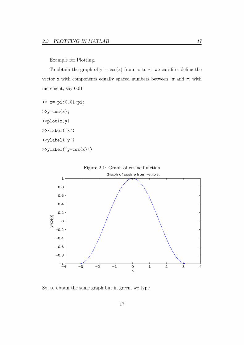
Example for Plotting.
To obtain the graph of y = cos(x) from -π to π, we can first define the
vector x with components equally spaced numbers between π and π, with
increment, say 0.01
>> x=-pi:0.01:pi;
>>y=cos(x);
>>plot(x,y)
>>xlabel(‘x’)
>>ylabel(‘y’)
>>ylabel(‘y=cos(x)’)
Figure 2.1: Graph of cosine function
−4 −3 −2 −1 0 1 2 3 4−1
−0.8
−0.6
−0.4
−0.2
0
0.2
0.4
0.6
0.8
1
x
y=co
s(x)
Graph of cosine from −π to π
So, to obtain the same graph but in green, we type
17

2.3. PLOTTING IN MATLAB 18
>>title(‘Graph of cosine from - \pi to \pi’)
>>plot(x,y,‘g’)
Figure 2.2: Graph of cosine function from −π to π
−4 −3 −2 −1 0 1 2 3 4−1
−0.8
−0.6
−0.4
−0.2
0
0.2
0.4
0.6
0.8
1
x
y=co
s(x)
Graph of cosine from −π to π
where the third argument indicating the color, appears within single quotes.
We could get a dashed line instead of a solid one by typing
>> plot(x,y,‘--’)
or even a combination of line type and color, say a blue dotted line by typing
>> plot(x,y,‘b:’)
Multiple curves can appear on the same graph. If for example we define
another vector
>> z = sin(x);
18
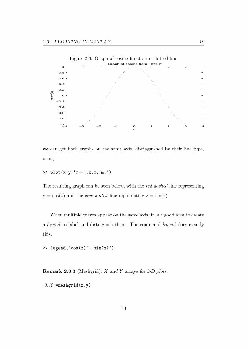
2.3. PLOTTING IN MATLAB 19
Figure 2.3: Graph of cosine function in dotted line
−4 −3 −2 −1 0 1 2 3 4−1
−0.8
−0.6
−0.4
−0.2
0
0.2
0.4
0.6
0.8
1
x
y=cos(
x)
Graph of cosine from −π to π
we can get both graphs on the same axis, distinguished by their line type,
using
>> plot(x,y,‘r--’,x,z,‘m:’)
The resulting graph can be seen below, with the red dashed line representing
y = cos(x) and the blue dotted line representing z = sin(x)
When multiple curves appear on the same axis, it is a good idea to create
a legend to label and distinguish them. The command legend does exactly
this.
>> legend(‘cos(x)’,‘sin(x)’)
Remark 2.3.3 (Meshgrid). X and Y arrays for 3-D plots.
[X,Y]=meshgrid(x,y)
19

2.3. PLOTTING IN MATLAB 20
Figure 2.4: Graph of cosine and sine functions
−4 −3 −2 −1 0 1 2 3 4−1
−0.8
−0.6
−0.4
−0.2
0
0.2
0.4
0.6
0.8
1cos(x)sin(x)
transforms the domain specified by vectors x and y into arrays X and Y that
can be used for the evaluation of function of two variables and 3D surface
plots.
The row of the output array X are copies of the vector x and the columns
of the output array Y are copies of the vector y.
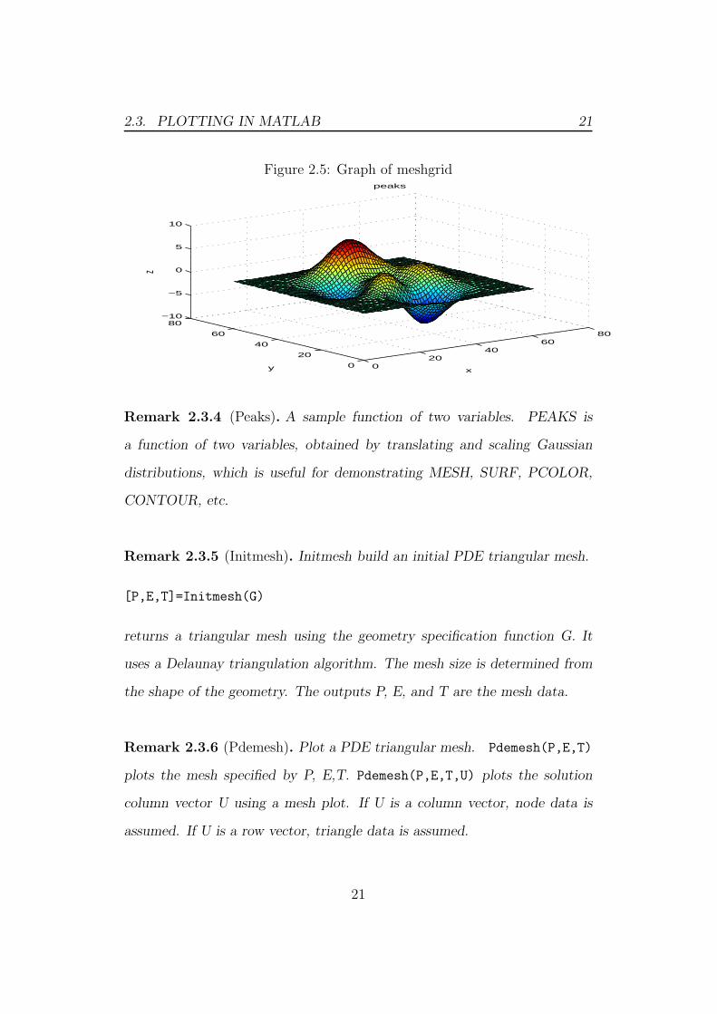
Example for Meshgrid.
>> [x,y] = meshgrid(-3:.1:3,-3:.1:3);
>> z = 3*(1-x).^2.*exp(-(x.^2) - (y+1).^2) ...
- 10*(x/5 - x.^3 - y.^5).*exp(-x.^2-y.^2) ...
- 1/3*exp(-(x+1).^2 - y.^2);
>> surf(z)
>> xlabel(‘x’)
>> ylabel(‘y’)
>> zlabel(‘z’)
>> title(‘Peaks’)
20
2.3. PLOTTING IN MATLAB 21
Figure 2.5: Graph of meshgrid
020
4060
80
0
20
40
60
80−10
−5
0
5
10
x
peaks
y
z
Remark 2.3.4 (Peaks). A sample function of two variables. PEAKS is
a function of two variables, obtained by translating and scaling Gaussian
distributions, which is useful for demonstrating MESH, SURF, PCOLOR,
CONTOUR, etc.
Remark 2.3.5 (Initmesh). Initmesh build an initial PDE triangular mesh.
[P,E,T]=Initmesh(G)
returns a triangular mesh using the geometry specification function G. It
uses a Delaunay triangulation algorithm. The mesh size is determined from
the shape of the geometry. The outputs P, E, and T are the mesh data.
Remark 2.3.6 (Pdemesh). Plot a PDE triangular mesh. Pdemesh(P,E,T)
plots the mesh specified by P, E,T. Pdemesh(P,E,T,U) plots the solution
column vector U using a mesh plot. If U is a column vector, node data is
assumed. If U is a row vector, triangle data is assumed.
21
2.3. PLOTTING IN MATLAB 22
Remark 2.3.7 (Pdesurf). Surface plot of PDE solution. Pdesurf(P,T,U)
plots a 3-D surface of PDE node or triangle data. If U is a column vector,
node data is assumed, and continuous style and interpolated shading are
used. If U is a row vector, triangle data is assumed, and discontinuous style
and flat shading are used.
Remark 2.3.8 (Assempde). Assemble the stiffness matrix and right hand
side a PDE problem. U=ASSEMPDE(B,P,E,T,C,A,F) assembles and solves
the PDE problem on a mesh described by P, E, and T, with boundary con-
ditions given by the function name B.
It eliminates the Dirichlet boundary conditions from the system of linear
equations when solving for U.
Remark 2.3.9 (Refinemesh). Refine a triangular mesh.
[P1,E1,T1]=REFINEMESH(G,P,E,T)
returns a refined version of the triangular mesh specified by the geometry G,
point matrix P, edge matrix E, and triangle matrix T.
22

Chapter 3
Numerical Methods for DE
3.1 Euler’s Method
Obtaining Approximations:
The object of Euler’s method is to obtain approximations to the well-posed
initial-value problem
dy
dt= f(t, y), a ≤ t ≤ b, y(a) = α
A continuous approximation to the solution y(t) will not be obtained; In-
stead, approximations to y will be generated at various values, called mesh
points, in the interval [a, b]. Once the approximate solution is obtained at
the points, the approximate solution at other points in the interval can
be found by interpolation. We first make the stipulation that the mesh
points are equally distributed throughout the interval [a, b]. This condition
is ensured by choosing a positive integer N and selecting the mesh points
ti = a + ih, for each i = 0, 1, 2, . . . , N . The common distance between the
points h =b− a
N= ti+1 − ti is called the step size.
23
3.1. EULER’S METHOD 24
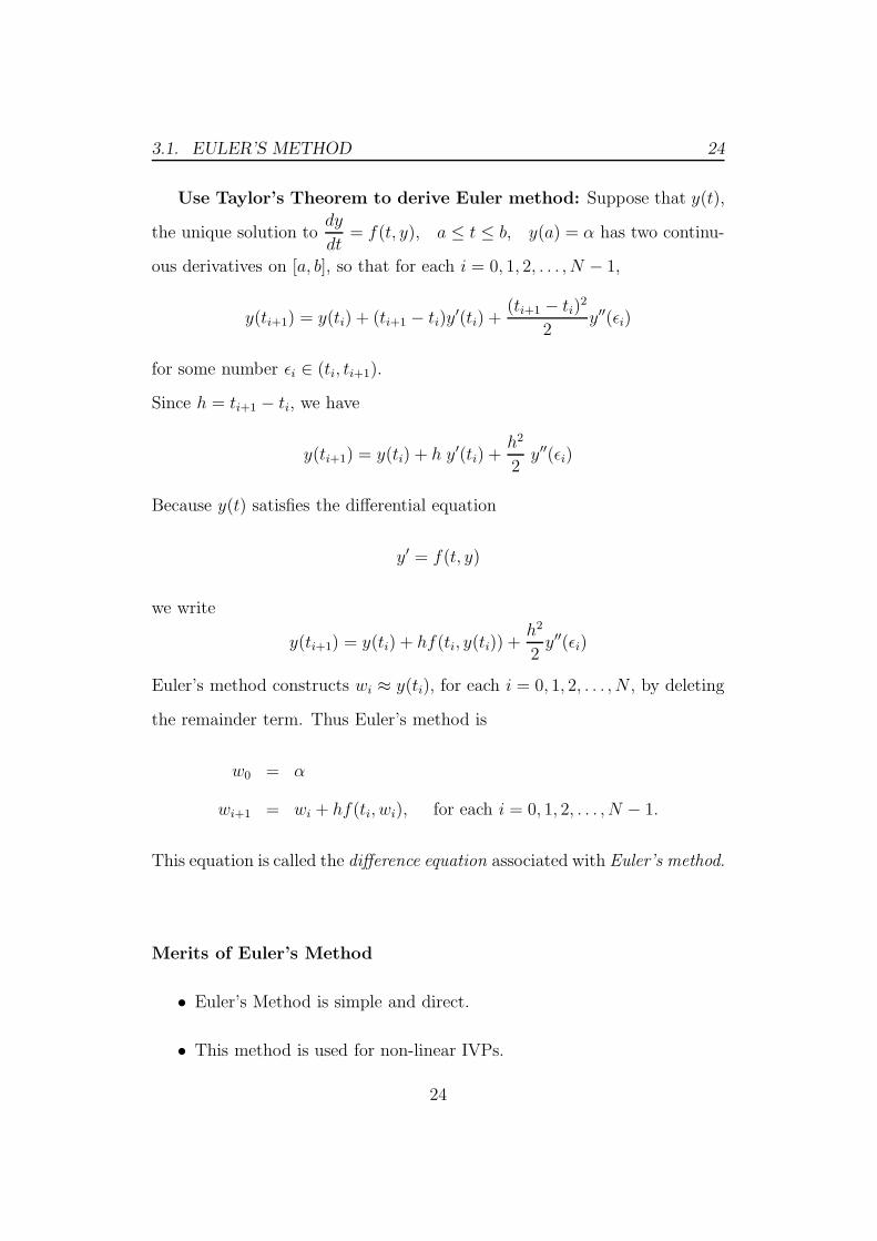
Use Taylor’s Theorem to derive Euler method: Suppose that y(t),
the unique solution tody
dt= f(t, y), a ≤ t ≤ b, y(a) = α has two continu-
ous derivatives on [a, b], so that for each i = 0, 1, 2, . . . , N − 1,
y(ti+1) = y(ti) + (ti+1 − ti)y′(ti) +
(ti+1 − ti)2
2y′′(ǫi)
for some number ǫi ∈ (ti, ti+1).
Since h = ti+1 − ti, we have
y(ti+1) = y(ti) + h y′(ti) +h2
2y′′(ǫi)
Because y(t) satisfies the differential equation
y′ = f(t, y)
we write
y(ti+1) = y(ti) + hf(ti, y(ti)) +h2
2y′′(ǫi)
Euler’s method constructs wi ≈ y(ti), for each i = 0, 1, 2, . . . , N , by deleting
the remainder term. Thus Euler’s method is
w0 = α
wi+1 = wi + hf(ti, wi), for each i = 0, 1, 2, . . . , N − 1.
This equation is called the difference equation associated with Euler’s method.
Merits of Euler’s Method
• Euler’s Method is simple and direct.
• This method is used for non-linear IVPs.
24

3.2. HEUN’S METHOD 25
Demerits of Euler’s Method
• It is less accurate and numerically unstable.
• Approximation error is proportional to the step size h. Hence, good
approximation is obtained with a very small h.
• This method requires a large number of time discretization leading to
a larger computation time.
• Usually applicable to explicit differential equations.
3.2 Heun’s Method
This method introduces a new idea for constructing an algorithm to solve
the I.V.P.
(1) y′(t) = f(t, y(t)) over [a, b] with y(t0) = y0.
To obtain the solution point (t1, y1), use the fundamental theorem of calculus
and integrate y′(t) over [t0, t1] to get,
(2)t1∫t0
f(t, y(t))dt =t1∫t0
y′(t)dt = y(t1)− y(t2)
the antiderivative of y′(t) is the desired function y(t). When equation (2) is
solved for y(t1), the result is
(3) y(t1) = y(t0) +t1∫t0
f(t, y(t))dt
A numerical integration method can be used to approximate the definite
integral in (3). If the trapezoidal rule is used with the step size h = t1 − t0,
then the result is
(4) y(t1) ≈ y(t0) +h
2(f(t0, y(t0))) + f(t1, y(t1))
25
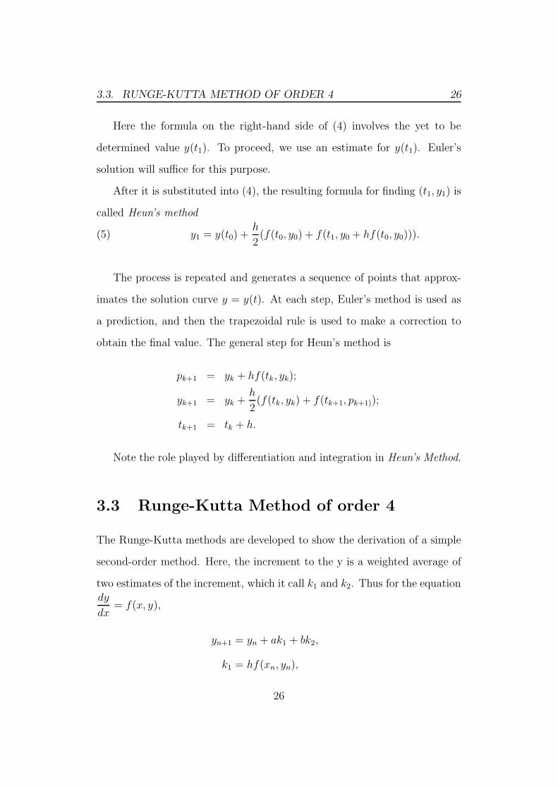
3.3. RUNGE-KUTTA METHOD OF ORDER 4 26
Here the formula on the right-hand side of (4) involves the yet to be
determined value y(t1). To proceed, we use an estimate for y(t1). Euler’s
solution will suffice for this purpose.
After it is substituted into (4), the resulting formula for finding (t1, y1) is
called Heun’s method
(5) y1 = y(t0) +h
2(f(t0, y0) + f(t1, y0 + hf(t0, y0))).
The process is repeated and generates a sequence of points that approx-
imates the solution curve y = y(t). At each step, Euler’s method is used as
a prediction, and then the trapezoidal rule is used to make a correction to
obtain the final value. The general step for Heun’s method is
pk+1 = yk + hf(tk, yk);
yk+1 = yk +h
2(f(tk, yk) + f(tk+1, pk+1));
tk+1 = tk + h.
Note the role played by differentiation and integration in Heun’s Method.
3.3 Runge-Kutta Method of order 4
The Runge-Kutta methods are developed to show the derivation of a simple
second-order method. Here, the increment to the y is a weighted average of
two estimates of the increment, which it call k1 and k2. Thus for the equation
dy
dx= f(x, y),
yn+1 = yn + ak1 + bk2,
k1 = hf(xn, yn),
26
3.3. RUNGE-KUTTA METHOD OF ORDER 4 27
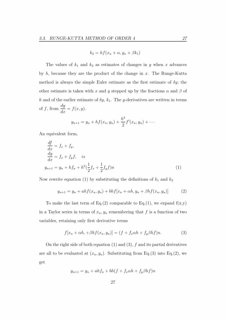
k2 = hf(xn + α, yn + βk1)
The values of k1 and k2 as estimates of changes in y when x advances
by h, because they are the product of the change in x. The Runge-Kutta
method is always the simple Euler estimate as the first estimate of δy; the
other estimate is taken with x and y stepped up by the fractions α and β of
h and of the earlier estimate of δy, k1. The y-derivatives are written in terms
of f , fromdy
dx= f(x, y).
yn+1 = yn + hf(xn, yn) +h2
2f ′(xn, yn) + · · ·
An equivalent form,
df
dx= fx + fy,
dy
dx= fx + fyf, is
yn+1 = yn + hfn + h2(1
2fx +
1
2fyf)n (1)
Now rewrite equation (1) by substituting the definitions of k1 and k2
yn+1 = yn + ahf(xn, yn) + bhf [xn + αh, yn + βhf(xn, yn)] (2)
To make the last term of Eq.(2) comparable to Eq.(1), we expand f(x,y)
in a Taylor series in terms of xn, yn remembering that f is a function of two
variables, retaining only first derivative terms
f [xn + αh,+βhf(xn, yn)] = (f + fxαh+ fyβhf)n. (3)
On the right side of both equation (1) and (3), f and its partial derivatives
are all to be evaluated at (xn, yn). Substituting from Eq.(3) into Eq.(2), we
get
yn+1 = yn + ahfn + bh(f + fxαh+ fyβhf)n
27

3.3. RUNGE-KUTTA METHOD OF ORDER 4 28
or rearranging
yn+1 = yn + (a + b)hfn + h2(αbfx + βbfyf)n (4)
Equation (4) will be identical to equation (1) if
a + b = 1, αb =1
2, βb =
1
2.
Note that only three equations need to be satisfied by the four unknowns.
This last set of parameters gives the modified Euler algorithm. This is a
special case of a second-order Runge-Kutta method.
Fourth-order Runge-Kutta methods are most widely used and are
derived similar. The set of 11 equations can be solved with 2 unknowns
being chosen arbitrarily. The most commonly used set of values lead to the
algorithm.
yn+1 = yn +1
6(k1 + 2k2 + 3k3 + k4),
k1 = hf(xn, yn),
k2 = hf(xn +1
2h, yn +
1
2k1),
k3 = hf(xn +1
2h, yn +
1
2k2),
k4 = hf(xn + h, yn + k2).
The local error term for the fourth order Runge-Kutta method is O(h5);
The global error would be O(h4). It is computationally more than the mod-
ified Euler Method.
Merits of Runge-Kutta Method
• This method is easy to implement.
• This method is stable.
28
3.4. RUNGE-KUTTA FEHLBERG METHOD 29
Demerits of Runge-Kutta Method
• This method requires relatively large computer time.
• Error estimation are not easy to be done.
• The Runge-Kutta methods do not work well for simple differential equa-
tions (eg. linear differential equations with widely spread eigenvalues).
• They are not good for systems of differential equations with a mix of
fast and slow state dynamics.
3.4 Runge-Kutta Fehlberg Method
The appropriate use of varying step size produce computationally efficient
integral approximating methods. In itself, this might not be sufficient to favor
these methods due to the increased complication of applying them. However,
they have another feature that makes them worthwhile. They incorporate
in the step-size procedure an estimate of the truncation error that does not
require the approximation of the higher derivatives of the function. These
methods are called adaptive because they adapt the number and position of
the nodes used in the approximation to ensure that the truncation error is
kept within a specified bound.
There is a close connection between the problem of approximating the
value of a definite integral and that of approximating the solution to an
initial-value problem. It is not surprising, then, that there are adaptive
methods for approximating the solutions to initial-value problems and that
these methods are not only efficient, but also incorporate the control of error.
29
3.4. RUNGE-KUTTA FEHLBERG METHOD 30
An ideal difference-equation method
wi+1 = wi + hiφ(ti, wi, hi), i = 0, 1, 2, . . . , N − 1.
for approximating the solution, y(t), to the initial-value problem
y′ = f(t, y), a < t < b, y(a) = α,
would have the property that, given a tolerance ǫ > 0, the minimal number
of mesh points would be used to ensure that the global error,| y(ti) − wi |,
would not exceed ǫ for any i = 0, 1, . . . , N . Having a minimal number of
mesh points and also controlling the global error of a difference method is,
not surprisingly, inconsistent with the points being equally spaced in the
interval. Now examine techniques used to control the error of a difference-
equation method in an efficient manner by the appropriate choice of mesh
points.
Although we cannot generally determine the global error of a method,
that there is a close connection between the local truncation error and the
global error. By using methods of differing order we can predict the local
truncation error and, using this prediction, choose a step size that will keep
it and the global error in check.
Suppose that we have two approximation techniques. The first is an
nth-order method obtained from an nth-order Taylor method of the form
y(ti+l) = y(ti) + hφ(ti, y(ti, h) +O(hn+1),
producing approximations
W0 = α,
Wi+l = Wi + hφ(ti,Wi, h), for i > 0,
30
3.4. RUNGE-KUTTA FEHLBERG METHOD 31
with local truncation error τi+1(h) = O(hn). In general, the method is gen-
erated by applying a Runge-Kutta modification to the Taylor method, but
the specific derivation is unimportant.
The second method is similar but one order higher; it comes from an
(n + l)st-order Taylor method of the form
y(ti+l) = y(ti) + hφ(ti, y(ti), h) +O(hn+2),
producing approximations
W0 = α,
Wi+l = Wi + hφ(ti, Wi, h), for i > 0,
with local truncation error τi+l(h) = O(hn+1).
Now first make the assumption that Wi ≈ y(ti) ≈ Wi and choose a fixed
step size h to generate the approximations Wi+1 and Wi+1 to y(ti+1). Then
τ i + 1 =y(ti+1)− y(ti)
h− φ(ti, y(ti), h)
=y(ti+1)− wi
h− φ(ti, wi, h)
=y(ti+1)− [wi + hφ(ti, wi, h)]
h
=1
h(y(ti+1)− wi+1)
In a similar manner,
τi+l(h) =1
h(y(ti+1)− wi+1)
and, as a consequence,
τi+1(h) =1
h(y(ti+1)−Wi+1)
=1
h[(y(ti+1 − Wi+1) + (Wi+1 −Wi+1)]
31
3.4. RUNGE-KUTTA FEHLBERG METHOD 32
= τi+1(h) +1
h(Wi+1 −Wi+1).
But τi+1(h) is O(hn) and τi+1(h) is O(hn+1), so the significant portion of
τi+1(h) must come from
1
h(wi+1 − wi+1)
This gives us an easily computed approximation for the local truncation error
of the 0(hn) method
τi+1(h) ≈1
h(wi+1 − wi+1)
The object is not simply to estimate the local truncation error but to adjust
the step size to keep it within a specified bound. We now assume that since
τi+1(h) is O(hn), a number K, independent of h, exists with
τi+1(h) ≈ Khn
Then the local truncation error produced by applying the nth-order method
with a new step size qh can be estimated using the original approximations
Wi+1 and Wi+1
τi+1(qh) ≈ K(qh)n = qn(khn) ≈ qnτi+1(h) ≈qn
h(Wi+1 −Wi+1)
To bound τi+1(qh) by ǫ, we choose q so that
qn
h| Wi+1 −Wi+1 |≈| τi+1(qh) |≤ ǫ
that is, so that
q ≤ (ǫh
| wi+1 − wi+1 |)1/n
One popular technique that uses this inequality for error control is the
Runge-Kutta-Fehlberg method. This technique uses a Runge-Kutta
method with local truncation error of order five,
Wi+1 = Wi +16
135k1 +
6656
12825k3 +
28561
56430k4 −
9
50k5 +
2
55k6
32
3.4. RUNGE-KUTTA FEHLBERG METHOD 33
to estimate the local error in a Runge-Kutta method of order four given by
Wi+1 = Wi +25
216k1 +
1408
2565k3 +
2197
4104k4 −
1
5k5
where,
k1 = hf(ti,Wi),
k2 = hf(ti +h
4,Wi +
1
4k1),
k3 = hf(ti +3h
8,Wi +
3
32k1 +
9
32k2),
k4 = hf(ti +12h
13,Wi +
1932
2197k1 +
7200
2197k2 +
7296
2197k3),
k5 = hf(ti + h,Wi +439
216k1 − 8k2 +
3680
513k3 −
845
4104k4),
k6 = hf(ti +h
2,Wi −
8
27k1 + 2k2 −
3544
2565k3 −
1859
4104k4 −
11
40k5).
with global error O(h5)
Error, E =k1360
− 128
4275k3 −
2197
75240k4 +
k550
+2
55k6
Merits of Runge-kutta-Fehlberg Method
• In this method, only six evaluations of f are required per step.
• Arbitrary Runge-Kutta methods of orders four and five used together
require at least four evaluations of f for the fourth-order method.
• In additional six for the fifth-order method, for a total of at least ten
functional evaluations.
33
Chapter 4
Solving Differential Equations
with MATLAB
MATLAB has an extensive library of functions for solving ordinary differ-
ential equations. Though MATLAB is primarily a numerics package, it can
certainly solve straight forward differential equations.
4.1 First Order Differential Equation
Example:
Solve the first order differential equation:
dy
dx(x) = xy; y(1) = 1
Solution:
>>y=dsolve(‘Dy=y*x’,‘x’)
y =
C2*exp(x^2/2)
34
4.1. FIRST ORDER DIFFERENTIAL EQUATION 35
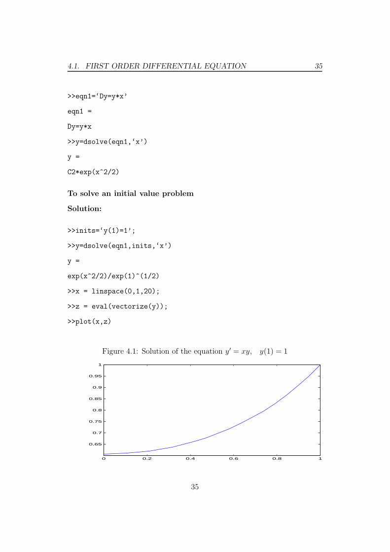
>>eqn1=‘Dy=y*x’
eqn1 =
Dy=y*x
>>y=dsolve(eqn1,‘x’)
y =
C2*exp(x^2/2)
To solve an initial value problem
Solution:
>>inits=‘y(1)=1’;
>>y=dsolve(eqn1,inits,‘x’)
y =
exp(x^2/2)/exp(1)^(1/2)
>>x = linspace(0,1,20);
>>z = eval(vectorize(y));
>>plot(x,z)
Figure 4.1: Solution of the equation y′ = xy, y(1) = 1
0 0.2 0.4 0.6 0.8 1
0.65
0.7
0.75
0.8
0.85
0.9
0.95
1
35
4.2. SECOND ORDER DIFFERENTIAL EQUATIONS 36
Now to use the same equation a number of times, we might choose to define
it as a variable, say eqn1.
There are two minor difficulties.
• Our expression for y(x) is not suited for array operations (.∗, ./, .∧)
• y, as MATLAB returns it, is actually a symbol.
To overcome these two difficulties, use Vectorize(). Vectorize() converts
symbolic objects into strings.
And use the command eval(), which evaluates or executes text strings.
4.2 Second Order Differential Equations
Example:
Solve and plot the solution of the second order equation:
d2ydx
(x) + 8 dydx(x) + 2y(x) = cos(x); y(0) = 0; y′(0) = 1.
Solution:
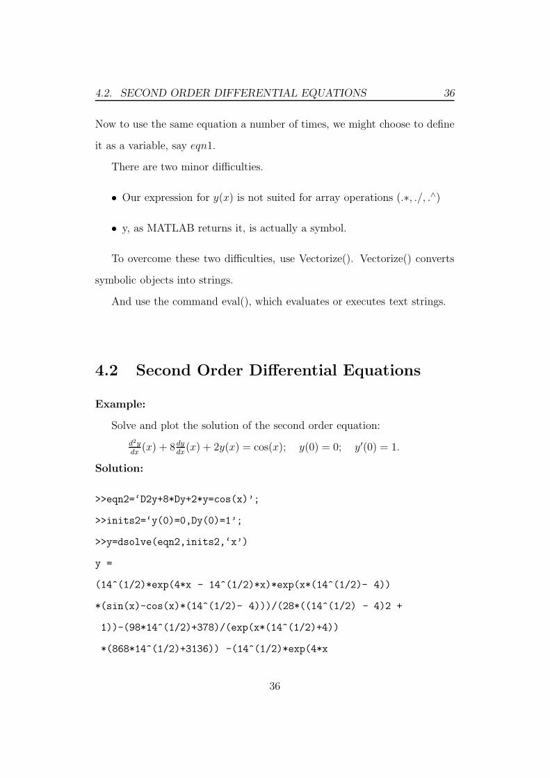
>>eqn2=‘D2y+8*Dy+2*y=cos(x)’;
>>inits2=‘y(0)=0,Dy(0)=1’;
>>y=dsolve(eqn2,inits2,‘x’)
y =
(14^(1/2)*exp(4*x - 14^(1/2)*x)*exp(x*(14^(1/2)- 4))
*(sin(x)-cos(x)*(14^(1/2)- 4)))/(28*((14^(1/2) - 4)2 +
1))-(98*14^(1/2)+378)/(exp(x*(14^(1/2)+4))
*(868*14^(1/2)+3136)) -(14^(1/2)*exp(4*x
36

4.3. SYSTEM OF DIFFERENTIAL EQUATIONS 37
+ 14^(1/2)*x)*(sin(x) +cos(x)*(14^(1/2)+ 4)))/
(28*exp(x*(14^(1/2)+4))*((14^(1/2)+4)^2 +1))
- (exp(x*(14^(1/2)- 4))*(98*14^(1/2)-378))
/(868*14^(1/2)-3136)
>>x=linspace(0,1,20);
>>z=eval(vectorize(y));
>>plot(x,z)
Figure 4.2: Solution of the DE y + 8y + 2y = cos(x) y(0) = 0 y′(0) = 1
0 0.2 0.4 0.6 0.8 10
0.02
0.04
0.06
0.08
0.1
0.12
0.14
0.16
0.18
0.2
4.3 System of Differential Equations
(1) Solve and plot solutions of the system of three ordinary differential equa-
tions:
x′(t) = x(t) + 2y(t)− z(t)
y′(t) = x(t) + z(t)
z′(t) = 4x(t)− 4y(t) + 5z(t)
37

4.3. SYSTEM OF DIFFERENTIAL EQUATIONS 38
Solution:
>>[x,y,z]=dsolve(‘Dx=x+2*y-z’,‘Dy=x+z’,‘Dz=4*x-4*y+5*z’)
x =
-(C3*exp(t))/2 -(C4*exp(2*t))/2 -(C5*exp(3*t))/4
y=
(C3*exp(t))/2 + (C4*exp(2*t))/4 + (C5*exp(3*t))/4
z =
C3*exp(t) + C4*exp(2*t) + C5*exp(3*t)
>>inits=‘x(0)=1,y(0)=2,z(0)=3’;
>>[x,y,z]=dsolve(‘Dx=x+2*y-z’,‘Dy=x+z’,‘Dz=4*x-4*y+5*z’,inits)
x =
6*exp(2*t) - (5*exp(3*t))/2 - (5*exp(t))/2
y =
(5*exp(3*t))/2 - 3*exp(2*t) + (5*exp(t))/2
z =
10*exp(3*t) - 12*exp(2*t) + 5*exp(t)
>>t=linspace(0,.5,25);
>>xx=eval(vectorize(x));
>>yy=eval(vectorize(y));
>>zz=eval(vectorize(z));
>>plot(t, xx, t, yy, t, zz)
To solve the Equation
dy
dx= xy2 + y; y(0) = 1.
We write the M-file firstode.m as follows
38

4.3. SYSTEM OF DIFFERENTIAL EQUATIONS 39
Figure 4.3: Solutions of x′ = x+ 2y − z, y′ = x+ z, z′ = 4x− 4y + 5z
0 0.1 0.2 0.3 0.4 0.50
5
10
15
20
25
function yprime = firstode(x,y);
yprime = x*y^2 + y;
>>xspan = [0,.5];
>>y0 = 1;
>>[x,y]=ode45(@firstode,xspan,y0);
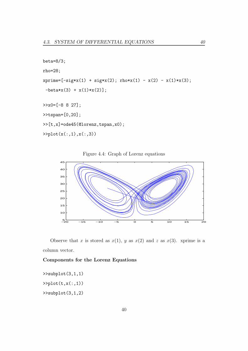
(2) Solve the system of Lorenz Equations:
dx
dt= −σx + σy
dy
dt= ρx− y − xz
dz
dt= −βx+ xy
Solution:
For the purpose of this problem we will take σ = 10, β = 83and ρ = 28
as well as x(0) = −8, y(0) = 8, z(0) = 27
function xprime = lorenz(t,x);
sig=10;
39
4.3. SYSTEM OF DIFFERENTIAL EQUATIONS 40
beta=8/3;
rho=28;
xprime=[-sig*x(1) + sig*x(2); rho*x(1) - x(2) - x(1)*x(3);
-beta*x(3) + x(1)*x(2)];
>>x0=[-8 8 27];
>>tspan=[0,20];
>>[t,x]=ode45(@lorenz,tspan,x0);
>>plot(x(:,1),x(:,3))
Figure 4.4: Graph of Lorenz equations
−20 −15 −10 −5 0 5 10 15 205
10
15
20
25
30
35
40
45
Observe that x is stored as x(1), y as x(2) and z as x(3). xprime is a
column vector.
Components for the Lorenz Equations
>>subplot(3,1,1)
>>plot(t,x(:,1))
>>subplot(3,1,2)
40
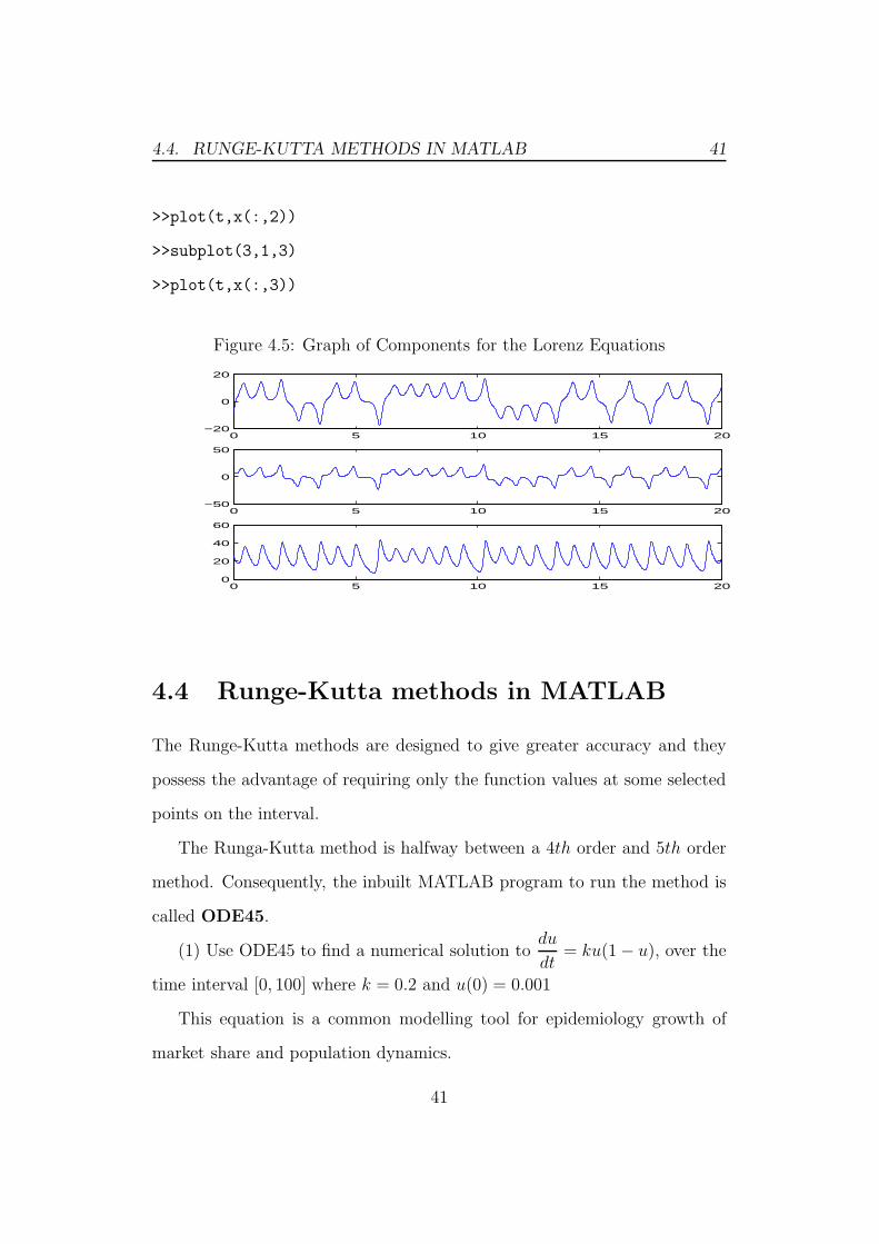
4.4. RUNGE-KUTTA METHODS IN MATLAB 41
>>plot(t,x(:,2))
>>subplot(3,1,3)
>>plot(t,x(:,3))
Figure 4.5: Graph of Components for the Lorenz Equations
0 5 10 15 20−20
0
20
0 5 10 15 20−50
0
50
0 5 10 15 200
20
40
60
4.4 Runge-Kutta methods in MATLAB
The Runge-Kutta methods are designed to give greater accuracy and they
possess the advantage of requiring only the function values at some selected
points on the interval.
The Runga-Kutta method is halfway between a 4th order and 5th order
method. Consequently, the inbuilt MATLAB program to run the method is
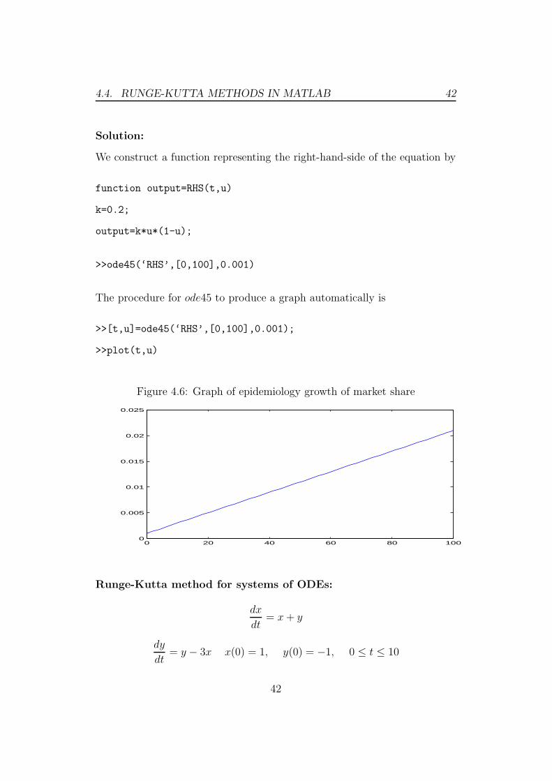
called ODE45.
(1) Use ODE45 to find a numerical solution todu
dt= ku(1− u), over the
time interval [0, 100] where k = 0.2 and u(0) = 0.001
This equation is a common modelling tool for epidemiology growth of
market share and population dynamics.
41
4.4. RUNGE-KUTTA METHODS IN MATLAB 42
Solution:
We construct a function representing the right-hand-side of the equation by
function output=RHS(t,u)
k=0.2;
output=k*u*(1-u);
>>ode45(‘RHS’,[0,100],0.001)
The procedure for ode45 to produce a graph automatically is
>>[t,u]=ode45(‘RHS’,[0,100],0.001);
>>plot(t,u)
Figure 4.6: Graph of epidemiology growth of market share
0 20 40 60 80 1000
0.005
0.01
0.015
0.02
0.025
Runge-Kutta method for systems of ODEs:
dx
dt= x+ y
dy
dt= y − 3x x(0) = 1, y(0) = −1, 0 ≤ t ≤ 10
42
4.4. RUNGE-KUTTA METHODS IN MATLAB 43
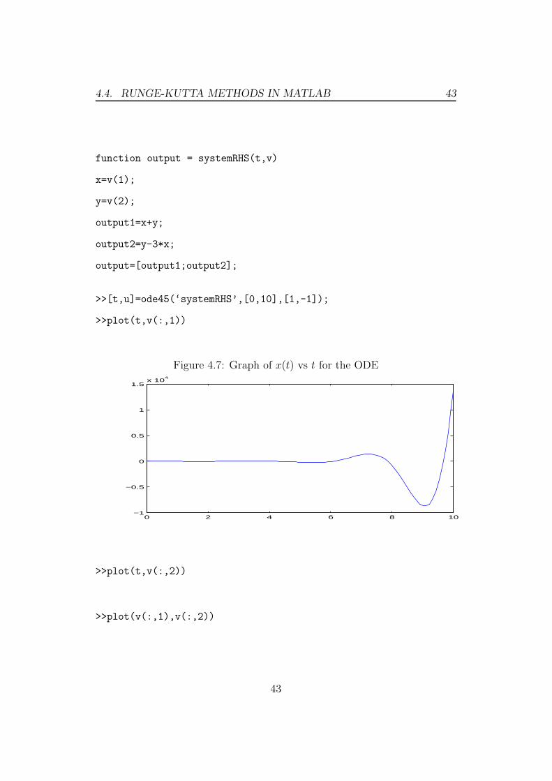
function output = systemRHS(t,v)
x=v(1);
y=v(2);
output1=x+y;
output2=y-3*x;
output=[output1;output2];
>>[t,u]=ode45(‘systemRHS’,[0,10],[1,-1]);
>>plot(t,v(:,1))
Figure 4.7: Graph of x(t) vs t for the ODE
0 2 4 6 8 10−1
−0.5
0
0.5
1
1.5x 10
4
>>plot(t,v(:,2))
>>plot(v(:,1),v(:,2))
43

4.4. RUNGE-KUTTA METHODS IN MATLAB 44
Figure 4.8: Graph of y vs t for the ODE
0 2 4 6 8 10−1
−0.5
0
0.5
1
1.5
2
2.5
3
3.5
4x 10
4
Figure 4.9: Graph of y vs x for the ODE
−1 −0.5 0 0.5 1 1.5
x 104
−1
−0.5
0
0.5
1
1.5
2
2.5
3
3.5
4x 10
4
44
4.5. EULER METHODS 45
4.5 Euler Methods
The Euler methods are simple methods of solving the first-order ODE, par-
ticularly suitable for quick programming because of their great simplicity,
although their accuracy is not high. Euler methods include three versions,
namely,
• Forward Euler method
• Modified Euler method
• Backward Euler method
Forward Euler Mehtod
If y′ = f(y, x) is derived by rewriting the forward difference approxima-
tion,
yn+1 − ynh
≈ y′n (4.1)
in to
yn+1 = yn + hf(yn, xn) (4.2)
where y′n = f(yn, xn) is used. In order to advance time steps, Eq. 4.2 is
recursively applied as
y1 = y0 + hy′0
y1 = y0 + hf(y0, x0)
y2 = y1 + hf(y1, x1)
y3 = y2 + hf(y2, x2)
. . . . . . . . .
yn = yn−1 + hf(yn−1, xn−1)
45
4.5. EULER METHODS 46
Modifed Euler method
The modifed Euler method is more accurate than the forward Euler
method. It is more stable. It is derived by applying the trapezoidal rule
to the solution of y′ = f(y, x)
yn+1 = yn +h
2[f(yn+1, xn+1) + f(yn, xn)] (4.3)
Backward Euler Method
The backward Euler method is based on the backward difference approx-
imation and written as
yn+1 = yn + hf(yn+1, xn+1) (4.4)
The accuracy of this method is quite the same as that of the forward Euler
method.
Euler Methods implemented in MATLAB
function [x,y]=euler_forward(f,xinit,yinit,xfinal,n)
h=(xfinal-xinit)/n;
x=[xinit zeros(1,n)]; y=[yinit zeros(1,n)];
for k=1:n
x(k+1)=x(k)+h;
y(k+1)=y(k)+h*f(x(k),y(k));
end
end
function [x,y]=euler_modified(f,xinit,yinit,xfinal,n)
h=(xfinal-xinit)/n;
46
4.5. EULER METHODS 47
x=[xinit zeros(1,n)];
y=[yinit zeros(1,n)];
for l=1:n
x(l+1)=x(l)+h;
ynew=y(l)+h*f(x(l),y(l));
y(l+1)=y(l)+(h/2)*(f(x(l),y(l))+f(x(l+1),ynew));
end
end
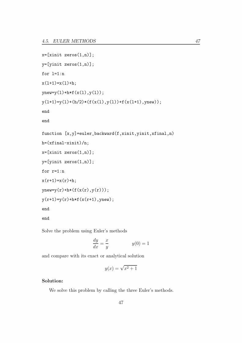
function [x,y]=euler_backward(f,xinit,yinit,xfinal,n)
h=(xfinal-xinit)/n;
x=[xinit zeros(1,n)];
y=[yinit zeros(1,n)];
for r=1:n
x(r+1)=x(r)+h;
ynew=y(r)+h*(f(x(r),y(r)));
y(r+1)=y(r)+h*f(x(r+1),ynew);
end
end
Solve the problem using Euler’s methods
dy
dx=
x
yy(0) = 1
and compare with its exact or analytical solution
y(x) =√x2 + 1
Solution:
We solve this problem by calling the three Euler’s methods.
47
4.5. EULER METHODS 48
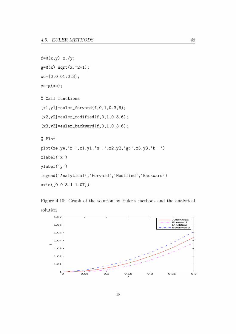
f=@(x,y) x./y;
g=@(x) sqrt(x.^2+1);
xe=[0:0.01:0.3];
ye=g(xe);
% Call functions
[x1,y1]=euler_forward(f,0,1,0.3,6);
[x2,y2]=euler_modified(f,0,1,0.3,6);
[x3,y3]=euler_backward(f,0,1,0.3,6);
% Plot
plot(xe,ye,‘r-’,x1,y1,‘m-.’,x2,y2,‘g:’,x3,y3,‘b--’)
xlabel(‘x’)
ylabel(‘y’)
legend(‘Analytical’,‘Forward’,‘Modified’,‘Backward’)
axis([0 0.3 1 1.07])
Figure 4.10: Graph of the solution by Euler’s methods and the analytical
solution
0 0.05 0.1 0.15 0.2 0.25 0.31
1.01
1.02
1.03
1.04
1.05
1.06
1.07
x
y
AnalyticalForwardModifiedBackward
48

4.5. EULER METHODS 49
% Estimate errors
error1=[‘Forward error:
‘ num2str(-100*(ye(end)-y1(end))/ye(end)) ‘%’]
error1 =
Forward error: -0.6751%
error2=[‘Modified error:
‘ num2str(-100*(ye(end)-y2(end))/ye(end)) ‘%’]
error2 =
Modified error: 0.0003983%
error3=[‘Backward error:
‘ num2str(-100*(ye(end)-y3(end))/ye(end)) ‘%’]
error3 =
Backward error: 0.67244%
Runge-Kutta Methods
There are many variants of the Runge-Kutta methods, but the most
widely used one is the following equation,
y′ = f(x, y)
y(xn) = yn
Solution
Now use this script file
f=@(x,y) x./y;
% Calculate exact solution
49
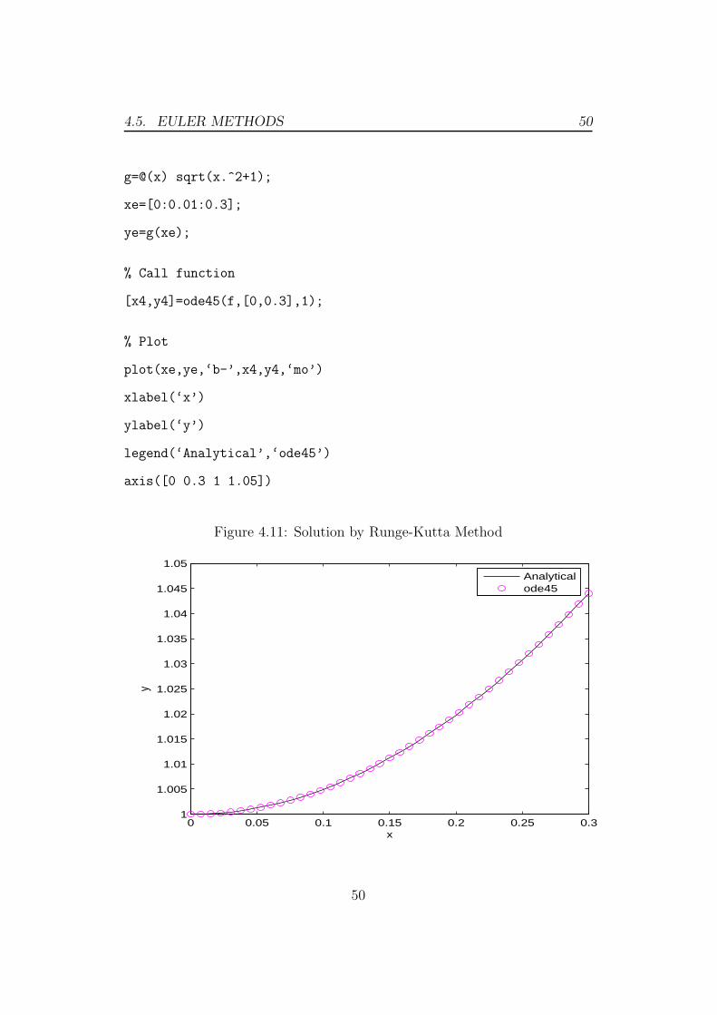
4.5. EULER METHODS 50
g=@(x) sqrt(x.^2+1);
xe=[0:0.01:0.3];
ye=g(xe);
% Call function
[x4,y4]=ode45(f,[0,0.3],1);
% Plot
plot(xe,ye,‘b-’,x4,y4,‘mo’)
xlabel(‘x’)
ylabel(‘y’)
legend(‘Analytical’,‘ode45’)
axis([0 0.3 1 1.05])
Figure 4.11: Solution by Runge-Kutta Method
0 0.05 0.1 0.15 0.2 0.25 0.31
1.005
1.01
1.015
1.02
1.025
1.03
1.035
1.04
1.045
1.05
x
y
Analyticalode45
50

Chapter 5
Comparison of numerical
approximations
We will now compare various methods and their approximation for 1st order
differential equation and a system of ODEs. We will test the problem with
the following methods: (1) Euler’s method, (2) Heun’s method, (3) RK4
method and (4) RKF5 method.
5.1 Comparison for a first order ODE
Consider the first order differential equation
y′(x) = f(x, y) = y + 2x− x2, y(0) = −1
The exact solution is given by
y(x) = x2 − ex
Now this problem is tested by various methods.
51
5.1. COMPARISON FOR A FIRST ORDER ODE 52
• Euler’s Method
• Heun’s Method
• RK4 Method
• RKF5 Method
with the interval x ∈ [0, 1]
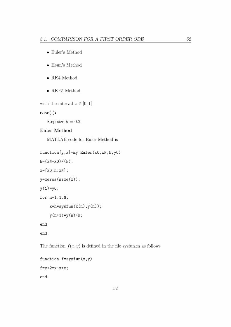
case(i):
Step size h = 0.2.
Euler Method
MATLAB code for Euler Method is
function[y,x]=my_Euler(x0,xN,N,y0)
h=(xN-x0)/(N);
x=[x0:h:xN];
y=zeros(size(x));
y(1)=y0;
for n=1:1:N,
k=h*sysfun(x(n),y(n));
y(n+1)=y(n)+k;
end
end
The function f(x, y) is defined in the file sysfun.m as follows
function f=sysfun(x,y)
f=y+2*x-x*x;
end
52

5.1. COMPARISON FOR A FIRST ORDER ODE 53
The exact solution is defined in a function as
function y=exact(x)
y=x.*x-exp(x);
end
The program should be called by the commands:
>>[y,x]=my_Euler(0,1,5,-1);
>>plot(x,exact(x),x,y,‘.’)
Figure 5.1: Solution of y = y + 2x− x2, y(0) = −1 by Euler’s Method
0 0.2 0.4 0.6 0.8 1−1.8
−1.7
−1.6
−1.5
−1.4
−1.3
−1.2
−1.1
−1
%Error tabulation
>>[x’,y’,exact(x’),abs(y’-exact(x’))]
ans =
0 -1.0000 -1.0000 0
0.2000 -1.2000 -1.1814 0.0186
53
5.1. COMPARISON FOR A FIRST ORDER ODE 54
0.4000 -1.3680 -1.3318 0.0362
0.6000 -1.5136 -1.4621 0.0515
0.8000 -1.6483 -1.5855 0.0628
1.0000 -1.7860 -1.7183 0.0677
Heun’s Method
MATLAB code for Heun’s Method is
function[y,x]=my_Heun(x0,xN,N,y0)
h=(xN-x0)/(N);
x=[x0:h:xN];
y=zeros(size(x));
y(1)=y0;
for n=1:1:N,
fn=sysfun(x(n),y(n));
k=y(n)+h*fn;
y(n+1)=y(n)+h/2*(fn+sysfun(x(n+1),k));
end
end
The program should be called by the commands:
>>[y2,x]=my_Heun(0,1,5,-1);
>>plot(x,exact(x),x,y2,‘*’);
%Error tabulation
>>[x’,y2’,exact(x’),abs(y2’-exact(x’))]
54
5.1. COMPARISON FOR A FIRST ORDER ODE 55
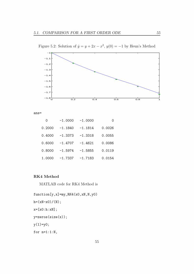
Figure 5.2: Solution of y = y + 2x− x2, y(0) = −1 by Heun’s Method
0 0.2 0.4 0.6 0.8 1−1.8
−1.7
−1.6
−1.5
−1.4
−1.3
−1.2
−1.1
−1
ans=
0 -1.0000 -1.0000 0
0.2000 -1.1840 -1.1814 0.0026
0.4000 -1.3373 -1.3318 0.0055
0.6000 -1.4707 -1.4621 0.0086
0.8000 -1.5974 -1.5855 0.0119
1.0000 -1.7337 -1.7183 0.0154
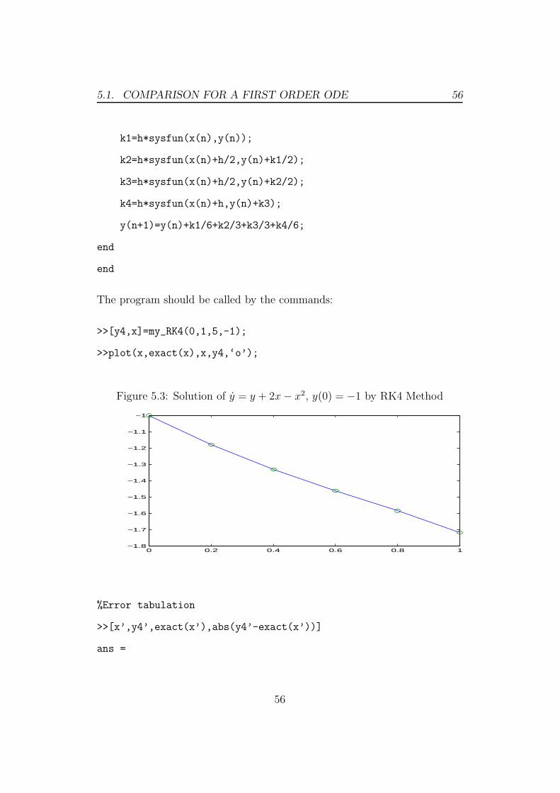
RK4 Method
MATLAB code for RK4 Method is
function[y,x]=my_RK4(x0,xN,N,y0)
h=(xN-x0)/(N);
x=[x0:h:xN];
y=zeros(size(x));
y(1)=y0;
for n=1:1:N,
55
5.1. COMPARISON FOR A FIRST ORDER ODE 56
k1=h*sysfun(x(n),y(n));
k2=h*sysfun(x(n)+h/2,y(n)+k1/2);
k3=h*sysfun(x(n)+h/2,y(n)+k2/2);
k4=h*sysfun(x(n)+h,y(n)+k3);
y(n+1)=y(n)+k1/6+k2/3+k3/3+k4/6;
end
end
The program should be called by the commands:
>>[y4,x]=my_RK4(0,1,5,-1);
>>plot(x,exact(x),x,y4,‘o’);
Figure 5.3: Solution of y = y + 2x− x2, y(0) = −1 by RK4 Method
0 0.2 0.4 0.6 0.8 1−1.8
−1.7
−1.6
−1.5
−1.4
−1.3
−1.2
−1.1
−1
%Error tabulation
>>[x’,y4’,exact(x’),abs(y4’-exact(x’))]
ans =
56
5.1. COMPARISON FOR A FIRST ORDER ODE 57
0 -1.0000 -1.0000 0
0.2000 -1.1814 -1.1814 0.0000
0.4000 -1.3318 -1.3318 0.0000
0.6000 -1.4621 -1.4621 0.0000
0.8000 -1.5856 -1.5855 0.0000
1.0000 -1.7183 -1.7183 0.0000
RKF5 Method
MATLAB code for RKF5 method is
function[y,x]=my_RKF5(x0,xN,N,y0)
h=(xN-x0)/(N);
x=[x0:h:xN];
y=zeros(size(x));
y(1)=y0;
R=[16/135,0,6656/12825,28561/56430,-9/50,2/55];
for n=1:1:N,
k1=h*sysfun(x(n),y(n));
k2=h*sysfun(x(n)+h/4,y(n)+k1/4);
k3=h*sysfun(x(n)+3*h/8,y(n)+3*k1/32+9*k2/32);
k4=h*sysfun(x(n)+12*h/13,y(n)+1932*k1/2197-7200*k2/2197
+7296*k3/2197);
k5=h*sysfun(x(n)+h,y(n)+439*k1/216-8*k2+3680*k3/513
-845*k4/4104);
k6=h*sysfun(x(n)+h/2,y(n)-8*k1/27+2*k2-3544*k3/2565
+1859*k4/4104-11*k5/40);
57

5.1. COMPARISON FOR A FIRST ORDER ODE 58
y(n+1)=y(n)+R(1)*k1+R(2)*k2+R(3)*k3+R(4)*k4+R(5)*k5
+R(6)*k6;
end
end
It should be called by the commands:
>>[y5,x]=my_RKF5(0,1,5,-1);
>>plot(x,exact(x),x,y5,‘+’);
Figure 5.4: Solution of y = y + 2x− x2, y(0) = −1 by RKF5 Method
0 0.2 0.4 0.6 0.8 1−1.8
−1.7
−1.6
−1.5
−1.4
−1.3
−1.2
−1.1
−1
%Error tabulation
>>[x’,y5’,exact(x’),abs(y5’-exact(x’))]
ans =
0 -1.0000 -1.0000 0
0.2000 -1.1814 -1.1814 0.0000
0.4000 -1.3318 -1.3318 0.0000
58

5.1. COMPARISON FOR A FIRST ORDER ODE 59
0.6000 -1.4621 -1.4621 0.0000
0.8000 -1.5855 -1.5855 0.0000
1.0000 -1.7183 -1.7183 0.0000
Comparison of Four Methods
Now we plot the solutions together in one figure, where the straight line
is the exact solution.
• the dot ‘.’ is the solution for Euler’s Method,
• the star ‘*’ is the solution for Heun’s Method,
• the circle ‘o’ is the solution for RK4 Method,
• the plus ‘+’ is the solution for RKF5 method.
>>x0=0;
>>x1=1;
>>N=5;
>>y0=-1;
>>[y,x]=my_Euler(x0,x1,N,y0);
>>[y2,x]=my_Heun(x0,x1,N,y0);
>>[y4,x]=my_RK4(x0,x1,N,y0);
>>[y5,x]=my_RKF5(x0,x1,N,y0);
>>ex=exact(x);
>>plot(x,ex,x,y,‘.’,x,y2,‘*’,x,y4,‘o’,x,y5,‘+’)
59

5.1. COMPARISON FOR A FIRST ORDER ODE 60
Figure 5.5: Comparison of four methods for an ODE (h = 0.2)
0 0.2 0.4 0.6 0.8 1−1.8
−1.7
−1.6
−1.5
−1.4
−1.3
−1.2
−1.1
−1
60
5.1. COMPARISON FOR A FIRST ORDER ODE 61
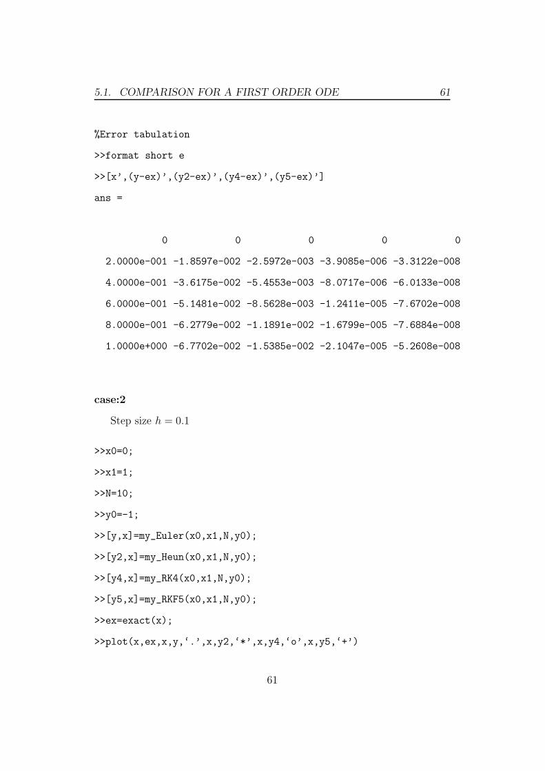
%Error tabulation
>>format short e
>>[x’,(y-ex)’,(y2-ex)’,(y4-ex)’,(y5-ex)’]
ans =
0 0 0 0 0
2.0000e-001 -1.8597e-002 -2.5972e-003 -3.9085e-006 -3.3122e-008
4.0000e-001 -3.6175e-002 -5.4553e-003 -8.0717e-006 -6.0133e-008
6.0000e-001 -5.1481e-002 -8.5628e-003 -1.2411e-005 -7.6702e-008
8.0000e-001 -6.2779e-002 -1.1891e-002 -1.6799e-005 -7.6884e-008
1.0000e+000 -6.7702e-002 -1.5385e-002 -2.1047e-005 -5.2608e-008
case:2
Step size h = 0.1
>>x0=0;
>>x1=1;
>>N=10;
>>y0=-1;
>>[y,x]=my_Euler(x0,x1,N,y0);
>>[y2,x]=my_Heun(x0,x1,N,y0);
>>[y4,x]=my_RK4(x0,x1,N,y0);
>>[y5,x]=my_RKF5(x0,x1,N,y0);
>>ex=exact(x);
>>plot(x,ex,x,y,‘.’,x,y2,‘*’,x,y4,‘o’,x,y5,‘+’)
61
5.1. COMPARISON FOR A FIRST ORDER ODE 62
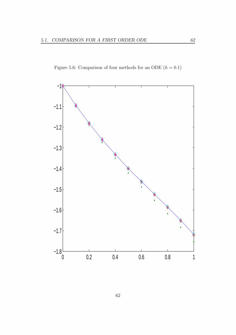
Figure 5.6: Comparison of four methods for an ODE (h = 0.1)
0 0.2 0.4 0.6 0.8 1−1.8
−1.7
−1.6
−1.5
−1.4
−1.3
−1.2
−1.1
−1
62

5.1. COMPARISON FOR A FIRST ORDER ODE 63
%Error tabulation
>>format short e
>>[x’,(y-ex)’,(y2-ex)’,(y4-ex)’,(y5-ex)’]
ans =......x_n......Euler......Heun.........RK4.......... RKF5
0 0 0 0 0
1.0000e-001 -4.8291e-003 -3.2908e-004 -1.2359e-007 -5.2611e-010
2.0000e-001 -9.5972e-003 -6.7474e-004 -2.5127e-007 -1.0099e-009
3.0000e-001 -1.4241e-002 -1.0368e-003 -3.8252e-007 -1.4368e-009
4.0000e-001 -1.8685e-002 -1.4150e-003 -5.1670e-007 -1.7892e-009
5.0000e-001 -2.2840e-002 -1.8086e-003 -6.5295e-007 -2.0470e-009
6.0000e-001 -2.6598e-002 -2.2167e-003 -7.9024e-007 -2.1863e-009
7.0000e-001 -2.9836e-002 -2.6380e-003 -9.2727e-007 -2.1792e-009
8.0000e-001 -3.2407e-002 -3.0708e-003 -1.0625e-006 -1.9935e-009
9.0000e-001 -3.4139e-002 -3.5128e-003 -1.1940e-006 -1.5918e-009
1.0000e+000 -3.4835e-002 -3.9613e-003 -1.3194e-006 -9.3046e-010
Now we compare the errors at the point xn = 0.1. We see that when we
half the step size,
• the error for Euler’s Method becomes circa 1/2.
• the error for Heun’s Method, it is circa 1/4 = 1/22.
• the error for RK4 Method, it is circa 1/16 = 1/24.
• the error for RKF5 Method, it si circa 1/32 = 1/25
This shows that the Euler’s Method is 1st order, Heun’s Method is 2nd
order, RK4 Method is 4th order and RKF5 is a 5th order method.
63
5.2. COMPARISON FOR A SYSTEM OF ODES 64
5.2 Comparison for a system of ODEs
We solve the problem:
d2
dx+ 2
dy
dx+ 0.75y = 0, y(0) = 3, y′(0) = −2.5.
The exact solution is
y′(x) = y1(x) = 2e−0.5x + e−1.5x;
y′(x) = y2(x) = −e−0.5x − 1.5e−1.5x
Here, we define the system in a function as follows
function f=sysfunsys(x,y)
f=zeros(2,1);
f(1)=y(2);
f(2)=-2*y(2)-0.75*y(1);
end
The exact solution is defined in a function
function y=exactsys(x)
y1=2*exp(-0.5*x)+exp(-1.5*x);
y2=-exp(-0.5*x)-1.5*exp(-1.5*x);
y=[y1;y2];
end
Euler Method
The MATLAB code for Euler method is
64
5.2. COMPARISON FOR A SYSTEM OF ODES 65
function [y,x]=sys_Euler(x0,xN,N,y0)
h=(xN-x0)/(N);
x=[x0:h:xN];
y=zeros(length(y0),length(x));
y(:,1)=y0;
for n=1:1:N,
k=h*sysfunsys(x(n),y(:,n));
y(:,n+1)=y(:,n)+k;
end
end
Heun’s Method
The MATLAB code for Heun’s Method is
function [y,x]=sys_Heun(x0,xN,N,y0)
h=(xN-x0)/(N);
x=[x0:h:xN];
y=zeros(length(y0),length(x));
y(:,1)=y0;
for n=1:1:N,
fn=sysfunsys(x(n),y(:,n));
k=y(:,n)+h*fn;
y(:,n+1)=y(:,n)+h/2*(fn+sysfunsys(x(n+1),k));
end
end
RK4 Method
The MATLAB code for RK4 Method is
65
5.2. COMPARISON FOR A SYSTEM OF ODES 66
function[y,x]=sys_RK4(x0,xN,N,y0)
h=(xN-x0)/(N);
x=[x0:h:xN];
y=zeros(length(y0),length(x));
y(:,1)=y0;
for n=1:1:N,
k1=h*sysfunsys(x(n),y(:,n));
k2=h*sysfunsys(x(n)+h/2,y(:,n)+k1/2);
k3=h*sysfunsys(x(n)+h/2,y(:,n)+k2/2);
k4=h*sysfunsys(x(n)+h,y(:,n)+k3);
y(:,n+1)=y(:,n)+k1/6+k2/3+k3/3+k4/6;
end
end
RKF5 Method
The MATLAB code for RKF5 Method is
function [y,x]=sys_RKF5(x0,xN,N,y0)
h=(xN-x0)/(N);
x=[x0:h:xN];
y=zeros(length(y0),length(x));
y(:,1)=y0;
R=[16/135, 0, 6656/12825, 28561/56430, -9/50, 2/55];
for n=1:1:N,
k1=h*sysfunsys(x(n),y(:,n));
k2=h*sysfunsys(x(n)+h/4,y(:,n)+k1/4);
k3=h*sysfunsys(x(n)+3*h/8,y(:,n)+3*k1/32+9*k2/32);
66

5.2. COMPARISON FOR A SYSTEM OF ODES 67
k4=h*sysfunsys(x(n)+12*h/13,y(:,n)+1932*k1/2197
-7200*k2/2197+7296*k3/2197);
k5=h*sysfunsys(x(n)+h,y(:,n)+439*k1/216-8*k2
+3680*k3/513-845*k4/4104);
k6=h*sysfunsys(x(n)+h/2,y(:,n)-8*k1/27+2*k2
-3544*k3/2565+1859*k4/4104-11*k5/40);
y(:,n+1)=y(n)+R(1)*k1+R(2)*k2+R(3)*k3+R(4)*k4
+R(5)*k5+R(6)*k6;
end
end
Comparison of Four Methods
>>x0=0;
>>x1=1;
>>N=5;
>>y0=[3;-2.5];
>>[y1,x]=sys_Euler(x0,x1,N,y0);
>>[y2,x]=sys_Heun(x0,x1,N,y0);
>>[y4,x]=sys_RK4(x0,x1,N,y0);
>>[y5,x]=sys_RKF5(x0,x1,N,y0);
>>ex=exactsys(x);
>>subplot(2,1,1);
>>plot(x,ex(1,:),x,y1(1,:),‘+’,x,y2(1,:),‘*’,x,y4(1,:),‘o’,
x,y5(1,:),‘.’),ylabel(‘y1’)
>>subplot(2,1,2);
>>plot(x,ex(2,:),x,y1(2,:),‘+’,x,y2(2,:),‘*’,x,y4(2,:),‘o’,
67
5.2. COMPARISON FOR A SYSTEM OF ODES 68
x,y5(2,:),‘.’),ylabel(‘y2’)
Now we plot the solution together in a figure, where the straight line is
the exact solution.
• the dot ‘+’ is the solution for Euler’s Method,
• the star ‘o’ is the solution for Heun’s Method,
• the circle ‘*’ is the solution for RK4 Method,
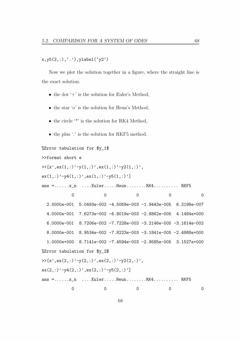
• the plus ‘.’ is the solution for RKF5 method.
%Error tabulation for $y_1$
>>format short e
>>[x’,ex(1,:)’-y(1,:)’,ex(1,:)’-y2(1,:)’,
ex(1,:)’-y4(1,:)’,ex(1,:)’-y5(1,:)’]
ans =......x_n ....Euler.....Heun........RK4.......... RKF5
0 0 0 0 0
2.0000e-001 5.0493e-002 -4.5069e-003 -1.9443e-005 6.2198e-007
4.0000e-001 7.6273e-002 -6.8019e-003 -2.8862e-005 4.1484e+000
6.0000e-001 8.7206e-002 -7.7228e-003 -3.2146e-005 -3.1614e-002
8.0000e-001 8.9534e-002 -7.8223e-003 -3.1841e-005 -2.4988e+000
1.0000e+000 8.7141e-002 -7.4594e-003 -2.9585e-005 3.1527e+000
%Error tabulation for $y_2$
>>[x’,ex(2,:)’-y(2,:)’,ex(2,:)’-y2(2,:)’,
ex(2,:)’-y4(2,:)’,ex(2,:)’-y5(2,:)’]
ans =......x_n ....Euler.....Heun........RK4.......... RKF5
0 0 0 0 0
68

5.2. COMPARISON FOR A SYSTEM OF ODES 69
Figure 5.7: Comparison of four methods for a system of ODEs
0 0.2 0.4 0.6 0.8 1−2
0
2
4
6
y1
0 0.2 0.4 0.6 0.8 1−5
0
5
y2
69

5.2. COMPARISON FOR A SYSTEM OF ODES 70
2.0000e-001 -6.6065e-002 6.4353e-003 2.9001e-005 -5.5000e+000
4.0000e-001 -9.6948e-002 9.6143e-003 4.2996e-005 2.3605e+000
6.0000e-001 -1.0717e-001 1.0785e-002 4.7816e-005 -5.5081e+000
8.0000e-001 -1.0586e-001 1.0770e-002 4.7275e-005 -2.9514e+000
1.0000e+000 -9.8631e-002 1.0099e-002 4.3828e-005 2.1544e+000
Now we see that errors are much smaller with higher order methods.
When h is halved, errors are smaller for all methods.
• For Euler’s Method it is circa 12.
• For Heun’s Method it is circa 14.
• For RK4 Method it is circa 116
• For RKF5 Method it is circa 1256
.
This agree with the theoretical result that the Euler’s Method is 1st order,
Heun’s Method is 2nd order, RK4Method is 4th order and RKF5 is 5th order.
70
Chapter 6
Solving Partial Differential
Equations with MATLAB
We solve the linear advection equation for u(x, t),
∂u
∂t= c
∂u
∂x
defined on (−∞,∞),t ∈ [0,∞) and with the boundary condition
u(x, 0) = f(x).
% Define and initialize the variables
for i = 1:10
xi(i) = i;
for j = 1:3
uij(i,j) = 0;
end
end
% The boundary condition (which essentially defines the "initial state")
71
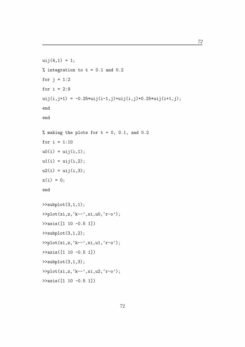
72
uij(4,1) = 1;
% integration to t = 0.1 and 0.2
for j = 1:2
for i = 2:9
uij(i,j+1) = -0.25*uij(i-1,j)+uij(i,j)+0.25*uij(i+1,j);
end
end
% making the plots for t = 0, 0.1, and 0.2
for i = 1:10
u0(i) = uij(i,1);
u1(i) = uij(i,2);
u2(i) = uij(i,3);
z(i) = 0;
end
>>subplot(3,1,1);
>>plot(xi,z,‘k--’,xi,u0,‘r-o’);
>>axis([1 10 -0.5 1])
>>subplot(3,1,2);
>>plot(xi,z,‘k--’,xi,u1,‘r-o’);
>>axis([1 10 -0.5 1])
>>subplot(3,1,3);
>>plot(xi,z,‘k--’,xi,u2,‘r-o’);
>>axis([1 10 -0.5 1])
72
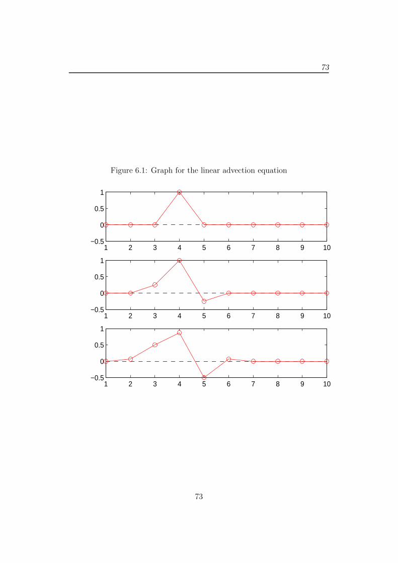
73
Figure 6.1: Graph for the linear advection equation
1 2 3 4 5 6 7 8 9 10−0.5
0
0.5
1
1 2 3 4 5 6 7 8 9 10−0.5
0
0.5
1
1 2 3 4 5 6 7 8 9 10−0.5
0
0.5
1
73

6.1. POISSON’S EQUATION ON A UNIT DISC 74
6.1 Poisson’s Equation on a Unit Disc
(1) Poisson’s Equation on a Unit Disk
The particular PDE is
−△ u = 1,
on the unit disk with zero-Dirichlet boundary conditions. The exact solution
is
u(x, y) =1− x2 − y2
4
Problem Definition:
The following variables will define our problem
• g: A specification function that is used by initmesh.
• b: A boundary file used by assempde.
• c,a,f: The coefficients and inhomogeneous term.
>>g=‘circleg’;
>>b=‘circleb1’;
>>c=1;
>>a=0;
>>f=1;
Generate Initial Mesh
The function initmesh takes a geometry specification function and returns
a discretization of that domain. The ‘hmax’ option lets the user specify the
maximum edge length. In this case, the domain is a unit disk, a maximum
edge length of one creates a coarse discretization.
74

6.1. POISSON’S EQUATION ON A UNIT DISC 75
[p,e,t]=initmesh(g,‘hmax’,1);
figure;
pdemesh(p,e,t);
axis equal
Figure 6.2: Graph for Poisson equation
−1 −0.5 0 0.5 1−1
−0.8
−0.6
−0.4
−0.2
0
0.2
0.4
0.6
0.8
1
Refinement
We repeatedly refine the mesh until the infinity-norm of the error vector
is less than a 10−3.
er = Inf;
while er > 0.001
[p,e,t]=refinemesh(g,p,e,t);
u=assempde(b,p,e,t,c,a,f);
exact=(1-p(1,:).^2-p(2,:).^2)’/4;
er=norm(u-exact,‘inf’);
fprintf(‘Error: %e. Number of nodes: %d\n’,er,size(p,2));
end
75
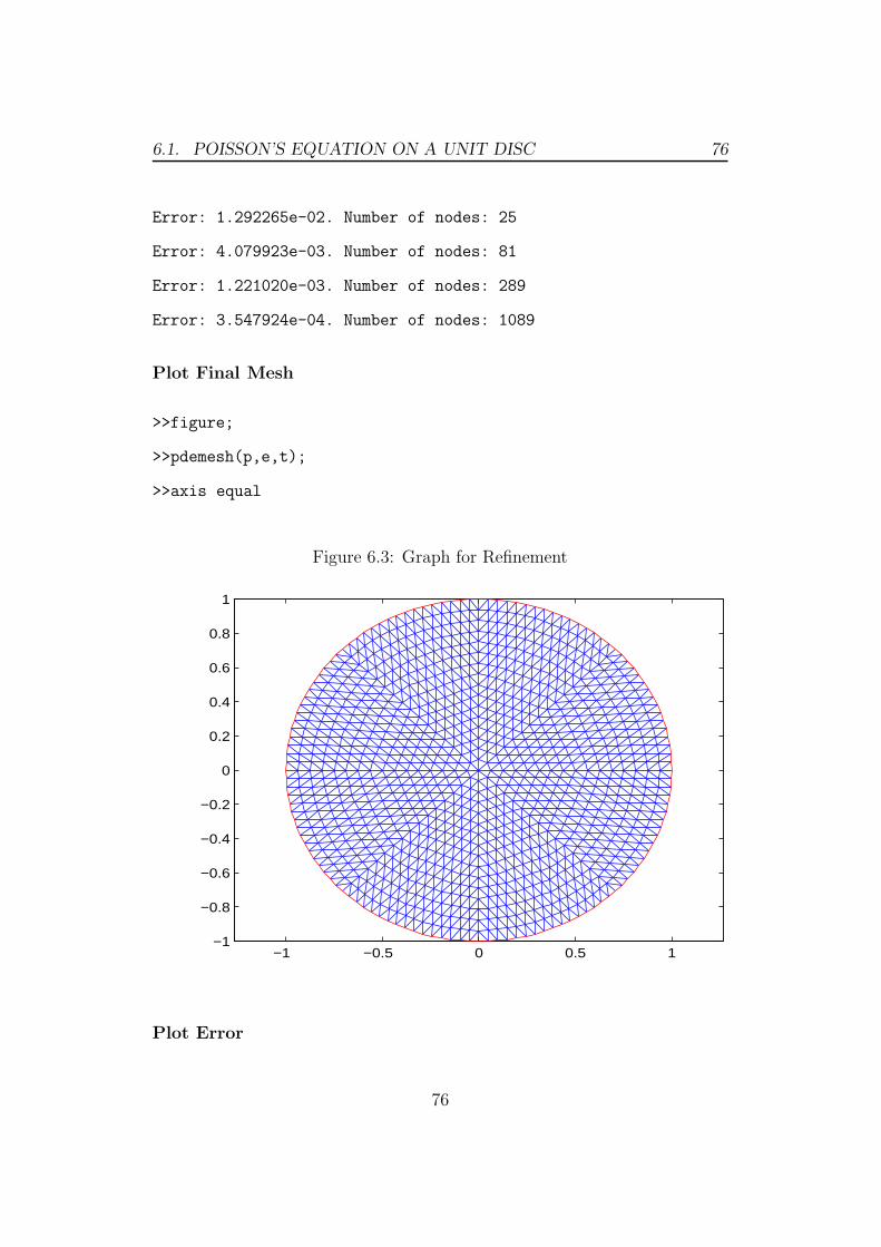
6.1. POISSON’S EQUATION ON A UNIT DISC 76
Error: 1.292265e-02. Number of nodes: 25
Error: 4.079923e-03. Number of nodes: 81
Error: 1.221020e-03. Number of nodes: 289
Error: 3.547924e-04. Number of nodes: 1089
Plot Final Mesh
>>figure;
>>pdemesh(p,e,t);
>>axis equal
Figure 6.3: Graph for Refinement
−1 −0.5 0 0.5 1−1
−0.8
−0.6
−0.4
−0.2
0
0.2
0.4
0.6
0.8
1
Plot Error
76

6.1. POISSON’S EQUATION ON A UNIT DISC 77
The scale of the vertical axis shows that the error is small and of the
order 10−4.
>>figure;
>>pdesurf(p,t,u-exact);
Figure 6.4: Graph for Exact
−1−0.5
00.5
1
−1
−0.5
0
0.5
1−1
0
1
2
3
4
x 10−4
Plot FEM Solution
>>figure;
>>pdesurf(p,t,u);
77
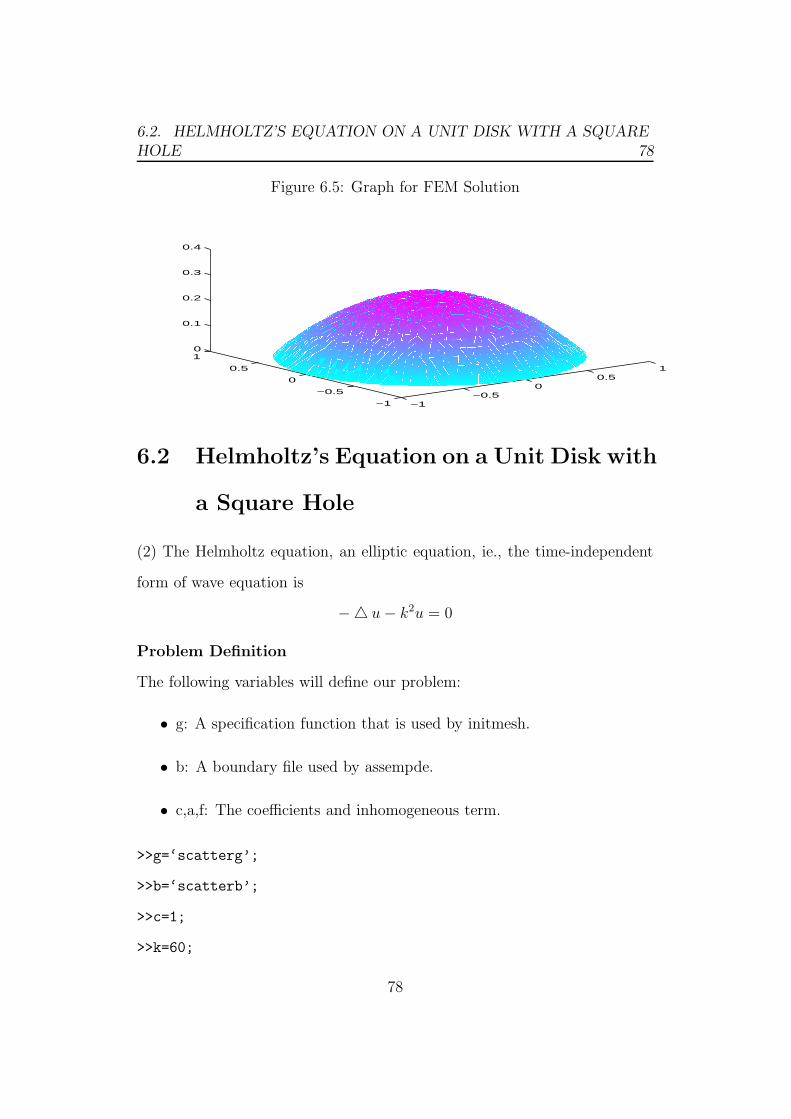
6.2. HELMHOLTZ’S EQUATION ON A UNIT DISK WITH A SQUAREHOLE 78
Figure 6.5: Graph for FEM Solution
−1−0.5
00.5
1
−1
−0.5
0
0.5
10
0.1
0.2
0.3
0.4
6.2 Helmholtz’s Equation on a Unit Disk with
a Square Hole
(2) The Helmholtz equation, an elliptic equation, ie., the time-independent
form of wave equation is
−△ u− k2u = 0
Problem Definition
The following variables will define our problem:
• g: A specification function that is used by initmesh.
• b: A boundary file used by assempde.
• c,a,f: The coefficients and inhomogeneous term.
>>g=‘scatterg’;
>>b=‘scatterb’;
>>c=1;
>>k=60;
78

6.3. SOLVE FOR COMPLEX AMPLITUDE 79
>>a=-k^2;
>>f=0;
Create Mesh
We need a fine mesh to resolve the waves. To achieve this, we refine the
initial mesh twice.
>>[p,e,t]=initmesh(g);
>>[p,e,t]=refinemesh(g,p,e,t);
>>[p,e,t]=refinemesh(g,p,e,t);
>>pdemesh(p,e,t);
axis equal
Figure 6.6: Graph for Helmholtz equation
0.4 0.6 0.8 1 1.2
0.1
0.2
0.3
0.4
0.5
0.6
0.7
0.8
0.9
6.3 Solve for Complex Amplitude
The real part of the vector u stores an approximation to a real-valued solution
of the Helmholtz equation.
>>u=assempde(b,p,e,t,c,a,f);
79
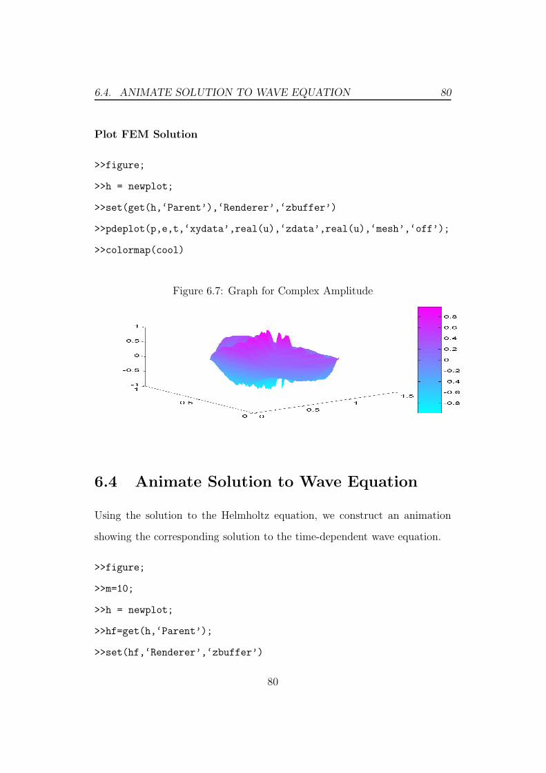
6.4. ANIMATE SOLUTION TO WAVE EQUATION 80
Plot FEM Solution
>>figure;
>>h = newplot;
>>set(get(h,‘Parent’),‘Renderer’,‘zbuffer’)
>>pdeplot(p,e,t,‘xydata’,real(u),‘zdata’,real(u),‘mesh’,‘off’);
>>colormap(cool)
Figure 6.7: Graph for Complex Amplitude
6.4 Animate Solution to Wave Equation
Using the solution to the Helmholtz equation, we construct an animation
showing the corresponding solution to the time-dependent wave equation.
>>figure;
>>m=10;
>>h = newplot;
>>hf=get(h,‘Parent’);
>>set(hf,‘Renderer’,‘zbuffer’)
80
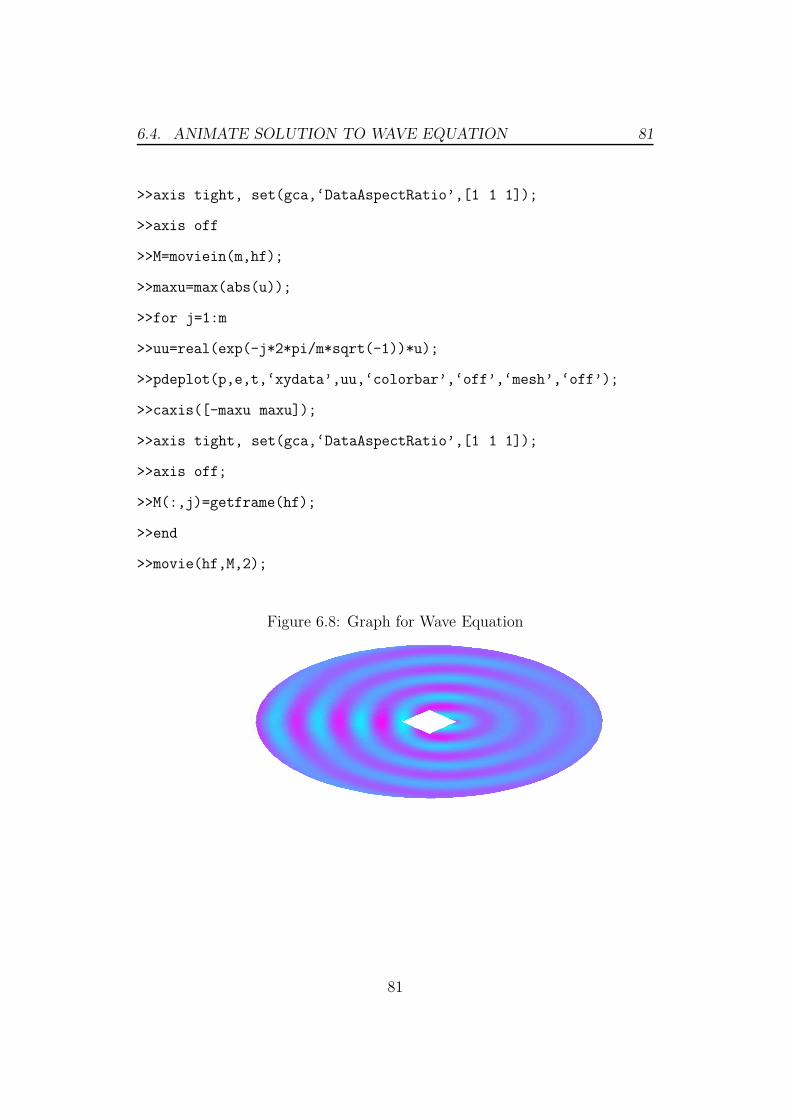
6.4. ANIMATE SOLUTION TO WAVE EQUATION 81
>>axis tight, set(gca,‘DataAspectRatio’,[1 1 1]);
>>axis off
>>M=moviein(m,hf);
>>maxu=max(abs(u));
>>for j=1:m
>>uu=real(exp(-j*2*pi/m*sqrt(-1))*u);
>>pdeplot(p,e,t,‘xydata’,uu,‘colorbar’,‘off’,‘mesh’,‘off’);
>>caxis([-maxu maxu]);
>>axis tight, set(gca,‘DataAspectRatio’,[1 1 1]);
>>axis off;
>>M(:,j)=getframe(hf);
>>end
>>movie(hf,M,2);
Figure 6.8: Graph for Wave Equation
81
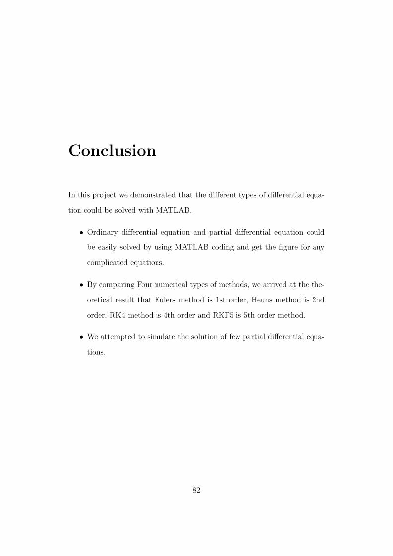
Conclusion
In this project we demonstrated that the different types of differential equa-
tion could be solved with MATLAB.
• Ordinary differential equation and partial differential equation could
be easily solved by using MATLAB coding and get the figure for any
complicated equations.
• By comparing Four numerical types of methods, we arrived at the the-
oretical result that Eulers method is 1st order, Heuns method is 2nd
order, RK4 method is 4th order and RKF5 is 5th order method.
• We attempted to simulate the solution of few partial differential equa-
tions.
82

Bibliography
[1] Curtis F. Gerald, Patrick O. Wheatley, “Applied Numerical Analysis”,
Addision-Wesley, Fifth Edition
[2] Wen Shen, “Journal on Introduction to Numerical computation”,
xuru.org, 2012.
[3] P.Howard, “Solving Ordinary Equations in MATLAB”, Fall, 2009.
[4] David Houcque, “Applications of MATLAB on Ordinary Differential
Equations”, Robert R. McCormick School of Engineering and Applied
Science, Northwestern University.
[5] Rudra Pratap, “Getting Started with MATLAB”, Department of Me-
chanical Engineering, Indian Institute of Science, Bangalore, 2010.
[6] Hari Kishan, “Differential Equations”, Atlantiv Publishers And Distrib-
utors, 2006.
83