A constitutive law for degrading bioresorbable polymers

Hassan Samami and Jingzhe Pan

Department of Engineering, University of Leicester, Leicester, UK

Abstract - This paper presents a constitutive law that predicts the

changes in elastic moduli, Poisson’s ratio and ultimate tensile strength of

bioresorbable polymers due to biodegradation. During biodegradation,

long polymer chains are cleaved by hydrolysis reaction. For semi-

cystalline polymers, the chain scissions also lead to crystallisation.

Treating each scission as a cavity and each new crystal as a solid

inclusion, a degrading semi-crystalline polymer can be modelled as a

continuum solid containing randomly distributed cavities and crystal

inclusions. The effective elastic properties of a degrading polymer are

calculated using existing theories for such solid and the tensile strength

of the degrading polymer is predicted using scaling relations that were

developed for porous materials. The theoretical model for elastic

properties and the scaling law for strength form a complete constitutive

relation for the degrading polymers. It is shown that the constitutive law

can capture the trend of the experimental data in the literature for a range

of biodegradable polymers fairly well.

Key words: effective moduli, cavity inclusion, crystal inclusion,

crystalline and amorphous polymers, multi-phase material.

1. Introduction

There is a worldwide attempt to develop and use bioresorbable medical implants such as

coronary stents and fixation screws made of bioresorbable polymers. The bioresorbable

screws and plates have been used for internal fixation in patients for a number of years. The

bioresorbable stents are currently being used in several countries. Unlike permanent implants

made of stainless steels or titanium alloys, bioresorbable implants “disappear” after serving

their functions in the human body. When designing bioresorbable implants, it is important to

understand how the mechanical properties of the polymer materials change as they degrade.

Degradation of bioresorbable polymers occurs by uptake of water and attack of water

molecules to ester bonds of the polymer chains in a time dependent process known as

hydrolysis degradation (Buchanan et al., 2008). The basic “damage” mechanism is polymer

chain scission caused by the hydrolysis reaction. These chain scissions lead to significant

reduction in the mechanical property of the polymers (Ashby and Jones, 2005, Tsuji, 2000,

Tsuji, 2002, Tsuji, 2003, Tsuji and Del Carpio, 2003, Tsuji and Muramatsu, 2001). Some

2

typical bioresorbable polymers are semi-crystalline. New nano-sized crystals can be formed

as the consequence of the extra mobility of the polymer chains due to chain scission. The

increase in crystallinity can be as high as 40% (Bouapao et al., 2009, Saha and Tsuji, 2006,

Tsuji et al., 2004). Because the crystals have a higher Young’s modulus than the amorphous

phase, the new crystals act as an enhancement phase that increases the Young’s modulus of

the semi-crystalline polymer. Despite a polymer chain cleavage is an event at the atomistic

scale, each chain-scission can be treated as an effective spherical cavity in the polymer. A

new crystal on the other hand can be treated as an inclusion of different Young’s modulus. It

is then possible to calculate the effective moduli of a degrading polymer for continuum solid

containing these cavities and inclusions. A representative volume element (RVE) for the

polymer is considered and it is assumed that the size of the cavities and crystals remains

constant, but their numbers increase as degradation proceeds. Gleadall (2014) performed such

calculations using finite element analysis. However the numerical calculations could only

provide empirical fitting equations for the Young’s modulus. These fitting functions are

unnecessarily dependent on the details of the finite element models. Furthermore Gleadall did

not consider the full constitutive response and ignored Poisson ratio and strength of

degrading polymers which are important if one wishes to use the constitutive law for device

design. This paper presents a complete and analytical constitutive law for degrading

polymers.

Numerous studies have been carried out for the effective moduli of composite materials. The

Voigt approximation is probably the simplest model which assumes the strain throughout a

composite is uniform and equal to the average strain. The Reuss approximation assumes that

the stress throughout a composite is uniform and equal to the average stress. Hill proved that

the Voigt approximation and Reuss approximation are actually the upper and lower bounds of

the effective elastic moduli (Hill, 1963). Hashin and Shtrikman also provided bounds for the

elastic moduli and tensors of isotropic composites reinforced by aligned continuous fibres or

randomly positioned particles which are similar to Walpole bounds but better than the Voigt

and Reuss bounds (Hashin and Shtrikman, 1962, Walpole, 1966). The effective moduli

estimated by Eshelby using the EIM method is only valid in the limit of low porosity (dilute

limit) (Eshelby, 1957). The EIM yields the same result as the dilute approximation which

ignores the interaction between reinforcing particles. The self-consistent schemes (SCS) use

material properties of a composite for infinite medium, i.e. the inclusion phase is assumed to

see an effective medium of unknown properties. Hill presented the overall constraint tensor

3

for an isotropic continuum containing a spherical cavity based on the self-consistent method.

He assumed that inclusions are spheres distributed in a way such that the composite is

statistically isotropic overall (Hill, 1963). Mackenzie (1950) was probably the first who

calculated the elastic constants of solid containing circular cavities. His scheme, known as the

generalised self-consistent scheme (GSCS), assumes that particles are surrounded by a

concentric shell of known property embedded in an effective medium of unknown properties

(Mackenzie, 1950). Buiansky proposed a method to avoid the problem of giving meaningless

values for the effective moduli of a composite material which arises when the volume

fraction of inhomogeneities is increased (Budiansky, 1965). The SCS is a two-phase model

while GSCS is a three-phase model which according to Aboudi yields a better result (Aboudi,

1991). Hashin also proposed a composite spheres model which derives the bulk modulus of a

composite material composed of a collection of spheres each of which consists of a spherical

core (particle) and a concentric spherical shell (matrix) (Hashin, 1962). The result of the

composite spheres model coincides with that of GSCS. The overall moduli of a two-phase

elastic composite material can also be determined by differential scheme (DS). In this method

the composite material is constructed explicitly from an initial material through a series of

incremental additions. To account for phase interaction effects, the Mori-Tanaka’s scheme

(MTS) relates the average stress or average strain tensors of matrix and inhomogeneities

(inclusion) phases by the fourth order concentration tensors (Mori and Tanaka, 1973). All of

the SCS, GSCS, DS and MTS schemes that are typically derived based on the concept of

representative volume element (RVE) are approximate schemes of interacting defects

(Kachanov et al., 1994). The RVE is a sub-volume of sufficient size of an inhomogeneous

medium. Since the material is assumed to be statistically homogeneous, the mechanical

properties of the entire composite material are assumed to be the same as those of the RVE.

This paper is structured as following: section 2 presents a model for predicting the effective

moduli of degrading crystalline polymers. The model of is also reduced to predict the

effective moduli of amorphous polymer. The effective moduli of several amorphous and

crystalline polymers are taken from the literature and fitted with the model in sections 3 and

4. Section 5 shows our calculation of the Poisson’s ratio for the same polymers considered in

sections 3 and 4. The tensile strength of these polymers is fitted using a scaling relation in

section 6.

4

2. A mathematical model for prediction of constitutive behaviour of degrading

bioresorbable polymers

Treating each chain-scission as an effective cavity, a degrading amorphous polymer can be

modelled by a continuum solid containing randomly distributed cavities with a common

radius. Fig. 1 shows a degrading polymer whose molecular chains are broken by hydrolysis

reactions. It is assumed that each chain scission leads to a cavity in the polymer matrix.

A semi-crystalline polymer undergoes an increased crystallinity during the hydrolysis

degradation (Tsuji et al., 2004). Treating each crystal as a solid inclusion and each chain

scission as a cavity, a degrading semi-crystalline polymer can be modelled by a continuum

solid containing cavities and solid inclusions. A crystal has a higher stiffness than the

amorphous matrix while a cavity is a region whose stiffness is zero.

Fig.2 shows our model for a degrading semi-crystalline polymer before and after degradation.

In the solid mechanics literature, the cavities and inclusions can be referred to as

inhomogeneity together. Fig.3 shows a representative volume element (RVE) of the solid

polymer subjected to uniformly remote stress 0 that contains an inhomogeneity )1( with

elastic stiffness )1(

IC (which is zero) and an inhomogeneity )2( whose elastic stiffness is

)2(

IC

. Since the size of the particles is much smaller compared to the size of the RVE, it can be

assumed with they don’t interact with the boundaries of the RVE.

The average stress of a 3-phase material with perfect bonding between constituents shown

as Fig. 3 can be obtained by (Aboudi, 1991, Mura, 1987).

𝜎 = 𝑓𝑀𝜎𝑀 + 𝑓𝐼(1)

𝜎𝐼(1)

+ 𝑓𝐼(2)

𝜎𝐼(2)

(1)

where Mf and )(

If are the volume fractions of the matrix and inhomogeneities, respectively.

Similarly, M and )( I are the average stress of the matrix and inhomogeneities (𝛼 = 1, 2),

respectively.

According to the average stress theorem when a uniform stress 0 is applied on the

boundary of this solid material, the average stress of the material is equal to 0 . Thus, Eq.

(1) becomes

5

𝜎0 = 𝑓𝑀𝜎𝑀 + 𝑓𝐼(1)

𝜎𝐼(1)

+ 𝑓𝐼(2)

𝜎𝐼(2)

(2)

Using Hook’s law Eq. (2) becomes

𝐶𝜀0 = 𝑓𝑀𝐶𝑀𝜀�̅� + 𝑓𝐼(1)

𝐶𝐼(1)

𝜀�̅�(1)

+ 𝑓(2)𝐶𝐼(2)

𝜀�̅�(2)

(3)

Where 𝐶𝑀 and 𝜀�̅� are the elastic stiffness and the average strain of the matrix phase. The

elastic stiffness of a cavity inclusion is 0)1( IC , Therefore, Eq. (3) reduces to

𝐶𝜀0 = 𝑓𝑀𝐶𝑀𝜀�̅� + 𝑓(2)𝐶𝐼(2)

𝜀�̅�(2)

(4)

From the analysis of the average strain we obtain

𝜀̅ = 𝑓𝑀𝜀�̅� + 𝑓𝐼(1)

𝜀�̅�(1)

+ 𝑓𝐼(2)

𝜀�̅�(2)

(5)

According to the average strain theorem 𝜀̅ = 𝜀0 (Mura, 1987), we have

𝑓𝑀𝜀�̅� = 𝜀0 − 𝑓𝐼(1)

𝜀�̅�(1)

− 𝑓𝐼(2)

𝜀�̅�(2)

(6)

Substitution of Eq. (6) into Eq. (4) gives the effective stiffness of degrading bioresorbable

polymers as

𝐶 = 𝐶𝑀 − 𝐶𝑀𝑓𝐼(1)

(𝜀�̅�(1)

/𝜀0) + (𝐶𝐼(2)

− 𝐶𝑀)𝑓𝐼(2)

(𝜀�̅�(2)

/𝜀0) (7)

In tensor notation form it can be written as

𝐶𝑖𝑗𝑘𝑙 = 𝐶𝑀𝑖𝑗𝑘𝑙− 𝐶𝑀𝑖𝑗𝑘𝑙

𝑓𝐼(1)

(𝜀�̅�𝑘𝑙

(1)/𝜀𝑘𝑙

0 ) + (𝐶𝐼𝑖𝑗𝑘𝑙

(2)− 𝐶𝑀𝑖𝑗𝑘𝑙

) 𝑓𝐼(2)

(𝜀�̅�𝑘𝑙

(2)/𝜀𝑘𝑙

0 ) (8)

This will be referred to as Model One in our following discussions, which is actually

constitutive law of effective moduli of a three phase particulate composite material when

𝐶𝐼𝑖𝑗𝑘𝑙

(1)= 0. It implies that the effective moduli of semi-crystalline bioresorbable polymers can

be determined from the elastic moduli of crystalline phase provided the average strain

𝜀�̅�𝑘𝑙

(𝛼) (𝛼 = 1, 2) in the phases are known.

The bulk and shear moduli when RVE is subjected to remote hydrostatic pressure 0

kk and

shear strain 0

12 are given by

𝐾 = 𝐾𝑀 − 𝐾𝑀𝑓𝐼(1)

(𝜀�̅�𝑘𝑘

(1)/𝜀𝑘𝑘

0 ) + (𝐾𝐼(2)

− 𝐾𝑀)𝑓𝐼(2)

(𝜀�̅�𝑘𝑘

(2)/𝜀𝑘𝑘

0 ) (9)

6

𝜇 = 𝜇𝑀 − 𝜇𝑀𝑓𝐼(1)

(𝜀�̅�12

(1)/𝜀12

0 ) + (𝜇𝐼(2)

− 𝜇𝑀)𝑓𝐼(2)

(𝜀�̅�12

(2)/𝜀12

0 ) (10)

The concentration factor 𝜀�̅�𝑖𝑗

(𝛼)/𝜀𝑖𝑗

0 can be determined from micro-mechanical schemes such as

MTS and EIM that can be found in Table 1.

The Poisson’s ratio and the Young modulus are given by

)3/(9 KKE (11)

)3(2/23 KK (12)

There are other schemes for the concentration factor in the literature. The reason to select

MTS and EIM models in this study is because EIM is valid for dilute limit and MTS also

accounts for the interaction between inclusions. Therefore, the result of Eq. (8) can be

compared with the both interacting and non-interacting inclusions.

The constitutive law for amorphous degrading polymer can be obtained from Eq. (8) by

setting 0)2( If as

𝐶𝑖𝑗𝑘𝑙 = 𝐶𝑀𝑖𝑗𝑘𝑙− 𝐶𝑀𝑖𝑗𝑘𝑙

𝑓𝐼(1)

(𝜀�̅�𝑘𝑙

(1)/𝜀0𝑘𝑙

) (13)

The bulk and shear moduli of the amorphous polymer are given by

𝐾 = 𝐾𝑀 − 𝐾𝑀𝑓𝐼(1)

(𝜀�̅�𝑘𝑘

(1)/𝜀0𝑘𝑘

) (14)

𝜇 = 𝜇𝑀 − 𝜇𝑀𝑓𝐼(1)

(𝜀�̅�12

(1)/𝜀012

) (15)

which is simply the constitutive law for the effective moduli of a two-phase composite

material when elastic moduli of the particles (phase 2) within the matrix phase is zero

(Aboudi, 1991, Mura, 1987). This will be referred to as Model Two in the following

discussion.

3. Predicting effective moduli of degrading amorphous polymers

The effective moduli of a degrading amorphous polymer can be calculated from Eq. (13)

using the initial conditions and the current average molecular weight of a degrading polymer.

The volume fraction of the cavities (porosity) (1/m3) is given by

sI Rrf 3)1( 4 (16)

7

where sR (mol m-3) is the number of chain-scissions, r (nm) is the radius of the cavities. The

radius r is the only fitting parameter in the model and unique to each polymer. The number of

chain-scissions, sR , can be obtained from the molecular weight using a relation developed by

Pan and co-workers (Pan, 2014).

sse

s

n

nn

Rm

RN

C

R

M

MM

0chain

00 1

1 (17)

0/ ess CRR ,

0

00

nchain

MN

(18)

where �̅�𝑛 is the number averaged molecular weight normalised by its initial value, 𝑀𝑛0 is

the initial number average molecular weight (g/mol), 𝐶𝑒0 is the initial concentration of ester

bonds (mol/m3), 𝛼 and 𝛽 are empirical parameters for oligomer production that depends on

the end or the random scissions (dimensionless), 0 is initial polymer density (g/m3), m is

the degree of polymerization of the oligomers (dimensionless and typically set as 4 to 6), Rs

is the total number of chain scissions per unit volume (mol/m3) and �̅�𝑠 is the total number of

chain scission normalised by the initial number of ester bond per unit volume. The molecular

weight can be either calculated using the polymer degradation model developed by Pan and

co-workers (Pan, 2014), or taken from experimental data in the literature which is what we

chose to do in the current paper. This eliminates the intermediate step of using the

degradation model since the purpose here to validate the constitutive law.

Table 2 shows the characteristics of four amorphous films made of poly(L-lactide) (PLLA),

poly(D-lactide) (PDLA) and poly(DL-lactide) (PDLLA) respectively that were used by Tsuji

etc al (Tsuji, 2002) in their degradation and mechanical experiments. All the initially

amorphous PLA films with 05.03018 3mm size were synthesized to have similar

molecular weight and to remain totally amorphous during 24 months hydrolysis degradation.

8

Table 2 also provides the radius of the effective cavities for each PLA films using which the

Young modulus of the PLA films are fitted using the MTS model.

The porosities of the PLA films of Table 2 as function of degradation time are obtained from

Eqs. (16) and (17) which are shown in Fig.4. It shows that the amorphous PDLLA polymer

has a higher porosity compared to other amorphous polymers.

Fig.5 shows the results of using Model Two for predicting the Young modulus of the PLA

films of Table 2. It shows that the model can capture the general trend of the experimental

data fairly well. Using average of the difference between normalised experimental and

predicted Young’s modulus data defined as 0.exp /)( EEEAverage Model gives a level of

agreement of 0.07, 0.05, 0.09 and 0.13 between experimental and predicted Young’s modulus

of the PLLA, PDLA, PDLLA and PDLA/PLLA films, respectively.

4. Predicting Young’s moduli of degrading semi-crystalline polymers

The effective moduli of the semi-crystalline crystalline polymers can be predicted from Eq.

(8). Similar to amorphous polymers the volume fraction of cavities is calculated from Eq.

(16). The volume fraction of the crystals can be obtained by using either the crystallisation

model (Gleadall et al., 2012, Han and Pan, 2008) or taking directly from experimental

measurements. Again we chose the latter since our aim here is to validate the constitutive

law. The number of chain scissions of a semi-crystalline polymer, sR , can be related to the

molecular weight and crystallinity using an equation proposed by Pan and co-workers (Pan,

2014).

sse

c

sc

n

nn

Rm

RN

CX

RX

M

MM

0chain

00

0

011

1 (19)

0

0

n

chainM

N

, 00 1

1

ce XC

(20)

9

where 0cX is the initial degree of crystallinity, is the number of the ester units of

crystalline phase per unit volume, 0chainN is the initial number of molecular chains per unit

volume including crystalline phase. Other symbols were introduced in section 3.

Error! Reference source not found. shows characteristics of different semi-crystalline

polymers used in different studies by various researchers. The first nine cases were taken

from the work by Tsuji and his co-workers (Tsuji and Ikada, 2000, Tsuji et al., 2000). These

were in two separate hydrolysis degradation studies in 10 ml phosphate-buffered solutions

over a period of 3 years. The case 10 shows a PLLA polymer used by Weir et al (Weir et al.,

2004) who used rod specimens for an in vitro hydrolytic degradation study over a period of

44 weeks. The PLLA polymers shown in cases 11-12 were also used as rod samples with 3

and 2 mm diameter, respectively, by Duek et al (Duek et al., 1999) for an vitro hydrolytic

degradation study over a period of 20 weeks.

Error! Reference source not found. also gives the radii of the cavities for each of the PLLA

films that were used to fit the constitutive law with the experimental data. It can be seen that

the PLLA films with higher crystallinity requires higher radius for the cavity. This agrees

with experimental observation that polymers with higher crystallinity absorb more water and

degrades faster (Tsuji and Ikada, 2000, Tsuji et al., 2000).

Fig. 6 shows the scission induced crystallinity (experimental data from the literature) and the

calculated porosity of polymer cases 1-13 of Table 3 as functions of degradation time.

Fig. 7 shows the fitting between the Model One and the experimental data for the first five

semi-crystalline PLLA films of Table 3. It can be observed from this figure that the model

can capture the trend of the experimental data fairly well, particularly for the first two years

of degradation during which the polymer loses 65% of its elastic property.

In fact, using the average of the difference between normalized experimental and predicted

Young’s modulus data shows that the level of agreement between experimental and predicted

Young’s modulus data is 0.11, 0.16, 0.19, 0.09 and 0.07 for the polymer cases 1-5 of Table 3.

Fig. 8 shows the fitting of the experimental data for Young modulus of the semi-crystalline

PLLA films of cases 6-9 of Table 3. It can be observed from this figure that the model can

again capture the general trend of the experimental Young modulus particularly for the semi-

crystalline PLLA cases 6 and 8 shown in Figs.8 (a) and (c). However, it cannot predict the

10

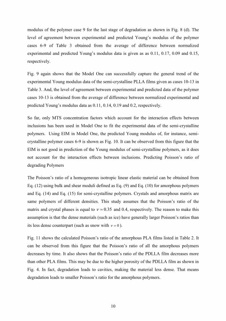
modulus of the polymer case 9 for the last stage of degradation as shown in Fig. 8 (d). The

level of agreement between experimental and predicted Young’s modulus of the polymer

cases 6-9 of Table 3 obtained from the average of difference between normalized

experimental and predicted Young’s modulus data is given as as 0.11, 0.17, 0.09 and 0.15,

respectively.

Fig. 9 again shows that the Model One can successfully capture the general trend of the

experimental Young modulus data of the semi-crystalline PLLA films given as cases 10-13 in

Table 3. And, the level of agreement between experimental and predicted data of the polymer

cases 10-13 is obtained from the average of difference between normalized experimental and

predicted Young’s modulus data as 0.11, 0.14, 0.19 and 0.2, respectively.

So far, only MTS concentration factors which account for the interaction effects between

inclusions has been used in Model One to fit the experimental data of the semi-crystalline

polymers. Using EIM in Model One, the predicted Young modulus of, for instance, semi-

crystalline polymer cases 6-9 is shown as Fig. 10. It can be observed from this figure that the

EIM is not good in prediction of the Young modulus of semi-crystalline polymers, as it does

not account for the interaction effects between inclusions. Predicting Poisson’s ratio of

degrading Polymers

The Poisson’s ratio of a homogeneous isotropic linear elastic material can be obtained from

Eq. (12) using bulk and shear moduli defined as Eq. (9) and Eq. (10) for amorphous polymers

and Eq. (14) and Eq. (15) for semi-crystalline polymers. Crystals and amorphous matrix are

same polymers of different densities. This study assumes that the Poisson’s ratio of the

matrix and crystal phases is equal to 35.0 and 0.4, respectively. The reason to make this

assumption is that the dense materials (such as ice) have generally larger Poisson’s ratios than

its less dense counterpart (such as snow with 0 ).

Fig. 11 shows the calculated Poisson’s ratio of the amorphous PLA films listed in Table 2. It

can be observed from this figure that the Poisson’s ratio of all the amorphous polymers

decreases by time. It also shows that the Poisson’s ratio of the PDLLA film decreases more

than other PLA films. This may be due to the higher porosity of the PDLLA film as shown in

Fig. 4. In fact, degradation leads to cavities, making the material less dense. That means

degradation leads to smaller Poisson’s ratio for the amorphous polymers.

11

The Poisson’s ratio of the semi-crystalline polymers listed in Table 5-3 is shown in Fig. 12. It

can be observed from this figure that the Poisson’s ratio of the semi-crystalline polymers

almost remains un-changed for an induction period then increases. The reason might be due

to the increase in crystallinity of the polymer at the later stage of degradation which causes

the polymer to become denser. Fitting tensile strength of degrading amorphous polymers

using scaling law

The experimental data of the tensile strength of degrading polymers can be predicted by using

the scaling relation of the porous metal foams from in the literature. This is particularly useful

in the early stage of design when approximate analysis of components and structures is

needed. The scaling relations for foam properties take the form (Ashby, 2000)

n

ssP

P

**

(21)

where P is a property (subscripted s means property of the matrix material (solid metal) and

superscript ‘*’ denotes the property of the foam), 𝛼 a constant and n a fixed exponent -they

depend on the structure of the foam and is the density. For instance, the tensile strength of

the porous metal foam scale with its density (Mg/m3) as

2/.3

,

s

sct

(22)

where 𝛼 has a value between 0.1 and 1.4, 𝜎𝑐,𝑠 is the initial compressive strength of the

matrix (solid metal), 𝜌/𝜌𝑠 is the material relative density and 𝜌𝑠 is density of the matrix.

The relative density of a degrading amorphous polymer due to the presence of cavities can be

expressed in terms of porosity as

)1(

0

1 If

(23)

where )1(

If is the density of cavities (porosity) that can be obtained from Eq. (16), is the

density of degrading polymer and 0 is the polymer density before degradation.

Using above relations the tensile strength of a degrading amorphous polymer can be

predicted by

12

nItt f )1(

0 1 (24)

where 0t is the initial tensile strength, has a value of 1 and n takes different values

depends on the polymer structure.

Applying Eq. (24) on amorphous PLLA, PDLA, PDLLA and PDLA/PLLA films listed in

Table 2 predicts their tensile strength as Fig.13. The PLA films have the same porosities C

as what obtained in section 4 (Fig. 4). That means the same radius of cavity r as what used in

section 4 for predicting the Young modulus of the PLA films is used here for the prediction

of the tensile strength of the PLA films. The values of r and n have been given in Table 4.

It can be observed from Fig. 23 that the scaling law can capture the trend of the experimental

tensile strength of the amorphous PLA films fairly well. Table 4 shows that PLA films with a

higher porosity have a higher value of n. In fact, the value of n governs by the density of the

degrading polymer which depends on the porosity of the polymer.

6.1 Sensitivity analysis

The sensitivity analysis shows that the tensile strength of the PLA films decreases faster

during the degradation time when r remains constant but n increases by 30% as shown in Fig.

24. This indicates that the tensile strength is not very sensitive to n.

However, when n remains constant but r increases by 30%, then the tensile strength of the

PLA films decreases much faster than when r remains constant but r increases by 30% as

shown in Fig.15. This indicates that the tensile strength is sensitive to r rather than n.

5. Conclusions

A complete constitutive law consisting of Model One and Model Two for elastic properties

and the scaling law for strength is presented to predict the change in elastic moduli, Poisson’s

ratio and ultimate tensile strength of bioresorbable polymers due to biodegradation. The

elastic moduli and Poisson’s ratio of semi-crystalline polymers having both initial and

scission-induced crystallinity were predicted by Model One which was also reduced to

predict the elastic moduli and Poisson’s ratio of the amorphous polymers referred to as Model

Two. The scaling law (that was derived based on the scaling relations for metal foam

13

properties) was used for fitting the tensile strength experimental data of degrading amorphous

bioresorbable polymers.

The results of the study showed that the constitutive law could successfully capture the trend

of the changes in observed mechanical properties of degrading bioresorbable polymers. It

also showed that the radius of cavities, r, which was the only fitting parameter in predicting

the elastic moduli of degrading polymers and used to calculate the porosity of such polymers,

had a value between 0.5-1.5 nm for amorphous polymers and 1.5-4.5 for semi-crystalline

polymers. Meanwhile, it was found out that the scaling law was very sensitive to r but not

much to another fitting parameter, n, that as a fixed exponent could take different values

depending on the polymer structure and was increasing when porosity of the degrading

polymers was decreasing.

Furthermore, the results showed that the degrading amorphous polymers with higher porosity

had a lower Poisson’s ratio. For instance, the Poisson’s ratio of the four amorphous PLA

films almost with 10%, 30%, 70% and 100% porosities after 2 year hydrolytic degradation

were decreased to about 4%, 13%, 23% and 30% respectively. The results also showed that

the Poisson’s ratio of the semi-crystalline polymers almost remained un-changed for an

induction period then increased. The reason might be due to the increase in the crystallinity of

the polymeric films which causes the polymers to become denser. In this study, the Poisson’s

ratio of the matrix and crystal phases was assumed to be 0.35 and 0.4, respectively. The

reason to make this assumption was that the dense materials (such as ice) have generally

larger Poisson’s ratios than its less dense counterpart (such as snow, 0 ).

Acknowledgement: This work is supported by a PhD studentship for Samami by the College

of Science of Engineering, the University of Leicester, which is gratefully acknowledged.

Appendix-Nomenclature

)( Inhomogeneities )2,1(

)(

IC Elastic stiffness of inhomogeneities

)(

IK Bulk modulus of inhomogeneities

)(I Shear modulus of inhomogeneities

)(If Volume fractions of inhomogeneities

)( I Average stress of inhomogeneities

14

)( I Average strain of inhomogeneities

Mf Volume fraction of matrix

MC Elastic stiffness of matrix

MK Bulk modulus of matrix

M Shear modulus of matrix

M Average stress of matrix

M Average strain of matrix

C Effective elastic stiffness of material

K Bulk modulus of the material

Shear moduli of material

Poisson’s ratio of material

Average stress of material

0 Uniform applied stress 0

kk Remote hydrostatic pressure

0

12 Remote shear strain

r Radius of cavities

nM Number averaged molecular weight normalised by its initial value

0nM Initial number average molecular weight (g/mol)

unitM Molecular weight of the repeating unit of the polymer chain (Kg/mol)

0eC Initial concentration of ester bonds (mol/m3)

, Empirical parameters for oligomer production (dimensionless)

Density (g/m3) of degrading polymer

0 Initial Polymer density (g/m3) (before degradation)

m Degree of polymerization of the oligomers (dimensionless)

sR Total number of chain-scissions per unit volume (mol/m3)

sR Total number of chain-scission normalised by initial number of ester bond per unit

volume

0cX Initial degree of crystallinity

cX Scission-induced crystallinity

Number of ester units of crystalline phase per unit volume

0chainN Initial number of molecular chains per unit volume including crystalline phase

0E Initial Young modulus

)2(

IE Young modulus of the crystals to fit the data

*P A property of the metal foam

sP A property of the matrix of metal foam

15

s Density of the matrix of metal foam

)1(

If Density of cavities (porosity)

A constant

t Tensile strength of the porous metal foam

0t Initial tensile strength

sc, Initial compressive strength of the matrix of metal foam

6. References

[1] ABOUDI, J. 1991. Mechanics of composite materials: a unified micromechanical

approach, Amsterdam, Elsevier.

[2] ASHBY, M. F. 2000. Metal foams: a design guide, Boston, Mass, Butterworth-

Heinemann.

[3] ASHBY, M. F. & JONES, D. R. H. 2005. Engineering materials 1: an introduction to

properties, applications and design, Amsterdam, Elsevier Butterworth-Heinemann.

[4] BOUAPAO, L., TSUJI, H., TASHIRO, K., ZHANG, J. & HANESAKA, M. 2009.

Crystallization, spherulite growth, and structure of blends of crystalline and

amorphous poly(lactide)s. Polymer, 50, 4007-4017.

[5] BUCHANAN, F., INSTITUTE OF MATERIALS, M. & MINING 2008. Degradation

rate of bioresorbable materials: prediction and evaluation, Cambridge, Woodhead

Publishing on behalf of the Institute of Materials, Minerals and Mining.

[6] BUDIANSKY, B. 1965. On the elastic moduli of some heterogeneous materials. Journal

of the Mechanics and Physics of Solids, 13, 223-227.

[7] DUEK, E. A. R., ZAVAGLIA, C. A. C. & BELANGERO, W. D. 1999. In vitro study of

poly(lactic acid) pin degradation. Polymer, 40, 6465-6473.

[8] ESHELBY, J. D. 1957. The Determination of the Elastic Field of an Ellipsoidal Inclusion,

and Related Problems. Proceedings of the Royal Society of London. Series A.

Mathematical and Physical Sciences, 241, 376-396.

16

[9] GLEADALL, A., PAN, J. & ATKINSON, H. 2012. A simplified theory of crystallisation

induced by polymer chain scissions for biodegradable polyesters. Polymer

Degradation and Stability, 97, 1616-1620.

[10] GLEADALL, A. 2014.Modelling degradation of biodegradable polymers and their

mechanical properties. PhD thesis. University of Leicester

[11] HAN, X. & PAN, J. 2008. A Model for Simultaneous Crystallisation and Biodegradation

of Biodegradable Polymers.

[12] HASHIN, Z. 1962. The Elastic Moduli of Heterogeneous Materials. Journal of Applied

Mechanics, 29, 143-150.

[13] HASHIN, Z. & SHTRIKMAN, S. 1962. A variational approach to the theory of the

elastic behaviour of polycrystals. Journal of the Mechanics and Physics of Solids, 10,

343-352.

[14] HILL, R. 1963. Elastic properties of reinforced solids: Some theoretical principles.

Journal of the Mechanics and Physics of Solids, 11, 357-372.

[15] KACHANOV, M., TSUKROV, I. & SHAFIRO, B. 1994. Effective Moduli of Solids

With Cavities of Various Shapes. Applied Mechanics Reviews, 47, S151-S174.

[16] LAM, K. H., NIEUWENHUIS, P., MOLENAAR, I., ESSELBRUGGE, H., FEIJEN, J.,

DIJKSTRA, P. J. & SCHAKENRAAD, J. M. 1994. Biodegradation of porous versus

non-porous poly(L-lactic acid) films. Journal of Materials Science: Materials in

Medicine, 5, 181-189.

[17] MACKENZIE, J. K. 1950. The Elastic Constants of a Solid containing Spherical Holes.

Proceedings of the Physical Society. Section B, 63, 2-11.

[18] MORI, T. & TANAKA, K. 1973. Average stress in matrix and average elastic energy of

materials with misfitting inclusions. Acta Metallurgica, 21, 571-574.

[19] MURA, T. 1987. Micromechanics of defects in solids, Lancaster, Nijhoff.

[20] PAN, J. 2014. Modelling Degradation of Bioresorbable Polymeric Medical Devices,

Burlington, Woodhead Publishing.

17

[21] SAHA, S. K. & TSUJI, H. 2006. Effects of rapid crystallization on hydrolytic

degradation and mechanical properties of poly( l-lactide-co-ε-caprolactone). Reactive

and Functional Polymers, 66, 1362-1372.

[22] SHODJA, H. M., RAD, I. Z. & SOHEILIFARD, R. 2003. Interacting cracks and

ellipsoidal inhomogeneities by the equivalent inclusion method. Journal of the

Mechanics and Physics of Solids, 51, 945-960.

[23] TSUJI, H. 2000. In vitro hydrolysis of blends from enantiomeric poly(lactide)s Part 1.

Well-stereo-complexed blend and non-blended films. Polymer, 41, 3621-3630.

[24] TSUJI, H. 2002. Autocatalytic hydrolysis of amorphous-made polylactides: effects of l-

lactide content, tacticity, and enantiomeric polymer blending. Polymer, 43, 1789-

1796.

[25] TSUJI, H. 2003. In vitro hydrolysis of blends from enantiomeric poly(lactide)s. Part 4:

well-homo-crystallized blend and nonblended films. Biomaterials, 24, 537-547.

[26] TSUJI, H. & DEL CARPIO, C. A. 2003. In vitro hydrolysis of blends from enantiomeric

poly(lactide)s. 3. Homocrystallized and amorphous blend films. Biomacromolecules,

4, 7-11.

[27] TSUJI, H. & IKADA, Y. 2000. Properties and morphology of poly( l-lactide) 4. Effects

of structural parameters on long-term hydrolysis of poly( l-lactide) in phosphate-

buffered solution. Polymer Degradation and Stability, 67, 179-189.

[28] TSUJI, H., IKARASHI, K. & FUKUDA, N. 2004. Poly( l-lactide): XII. Formation,

growth, and morphology of crystalline residues as extended-chain crystallites through

hydrolysis of poly( l-lactide) films in phosphate-buffered solution. Polymer

Degradation and Stability, 84, 515-523.

[29] TSUJI, H., MIZUNO, A. & IKADA, Y. 2000. Properties and morphology of poly(L-

lactide). III. Effects of initial crystallinity on long-term in vitro hydrolysis of high

molecular weight poly(L-lactide) film in phosphate-buffered solution. Journal of

Applied Polymer Science, 77, 1452-1464.

18

[30] TSUJI, H. & MURAMATSU, H. 2001. Blends of aliphatic polyesters: V non-enzymatic

and enzymatic hydrolysis of blends from hydrophobic poly( l-lactide) and hydrophilic

poly(vinyl alcohol). Polymer Degradation and Stability, 71, 403-413.

[31] WALPOLE, L. J. 1966. On bounds for the overall elastic moduli of inhomogeneous

systems—I. Journal of the Mechanics and Physics of Solids, 14, 151-162.

[32] WEIR, N. A., BUCHANAN, F. J., ORR, J. F. & DICKSON, G. R. 2004. Degradation

of poly-L-lactide. Part 1: in vitro and in vivo physiological temperature degradation.

Proceedings of the Institution of Mechanical Engineers.Part H, Journal of

engineering in medicine, 218, 307-319.

a) A long molecular chain

(before degradation)

b) Chain-cleavage c) Formation of cavities

due to chain-scission

Fig. 1: Assumption of using cavities to represent polymer chain cleavages

19

a) A long molecular chain with

initial crystallinity (before

degradation)

b) Chain-cleavage c) Formation of cavities and

crystals due to chain-scissions

and increased crystallinity

Fig.2: Assumption of using cavities and crystals to represent a degrading semi -

crystalline polymer

Inhomogeneities

Fig.3: The RVE containing two inhomogeneities with different stiffness (adapted

from (Shodja et al., 2003)

20

Fig.4: Porosity of PLA films of Table 2 as a function of time tested by Tsuji et al

(Tsuji, 2002)

Young’s modulus of amorphous PLA films of Table 2

Fig.5: Fitting of Young modulus as a function of degradation time using MTS model

with experimental data obtained by Tsuji et al (Tsuji, 2002) for amorphous PLLA,

PDLA, PDLLA and PLLA/PDLA films

21

Porosity and crystallinity of semi-crystalline PLLA films of Table 5-3

22

Fig. 6: Crystallinity (experimental data) and porosity (calculated) of semi -

crystalline PLLA films (cases 1-13 of Table 3)

23

Young’s modulus of semi-crystalline PLLA films cases 1-5 of Table 3

Fig. 7: Fitting of experimental data of Young modulus of polymer cases 1-5 of Table

3 using Model One with MTS concentration factors. The experimental data were

taken from (Tsuji et al., 2000)

24

Young’s modulus of semi-crystalline PLLA films cases 6-9 of Table 3

Fig. 8: Fitting of experimental data of Young modulus of semi-crystalline PLLA

polymers of cases 6-9 of Table 3 using MTS concentration factors in Model One. The

experimental data were taken from (Tsuji and Ikada, 2000)

25

Young's modulus of semi-crystalline PLLA films cases 10-13 of Table 3

Fig. 9: Fitting of experimental data of Young modulus of semi-crystalline PLLA

polymer (case 10-13 of Table 3) using Model One with MTS concentration factors

26

Fig. 10: Fitting of experimental data of Young modulus of semi-crystalline PLLA

polymers (cases 6-9 of Table 3) using Model One with EIM concentration factors

27

Fig. 11: Calculated Poisson’s ratio of amorphous PLLA, PDLA, PDLLA and

PDLA/PLLA films (listed in table 2) as function of degradation time over 24 months

28

Poisson’s ratio of semi-crystalline PLLA films of Table 3

(a) Cases 1-5 (b) Cases 6-9

(c) Case 10 (d) Cases 11 & 12

(e) Case 13

Fig. 12: Calculated Poisson’s ratio of semi-crystalline PLLA films of cases 1-13 of

Table 3

29

Fig.13: Fitting of the tensile strength of the amorphous PLA films of Table 2 using

scaling law

30

Fig.14: Tensile strength of the amorphous PLA films of Table2 when r remains

constant but n increases by 30%

31

Fig.15: Tensile strength of the amorphous PLA films of Table2 when r increases by

30% but n remains constant

32

Table 1: Concentration factor of EIM and MTS schemes for elastic spherical

inclusions (Aboudi, 1991, Mura, 1987)

Concentration

factors EIM MTS

ε̅I12

(1)/ε12

0 15(1 − 𝜈0)

(7 − 5𝜈0)

1

−6(𝐾𝑀 + 2𝜇𝑀) 1 − 𝑓𝐼

(1)

5(3𝐾𝑀 + 4𝜇𝑀)+ 1

ε̅Ikk

(1)/εkk

0 3(𝜈0 − 1)

2(2𝜈0 − 1)

1

−3 1 − 𝑓𝐼

(1) 𝐾𝑀

(3𝐾𝑀 + 4𝜇𝑀)+ 1

ε̅I12

(2)/ε12

0 15(1 − 𝜈0)𝜇𝑀

(7 − 5𝜈0)𝜇𝑀 + 2(4 − 5𝜈0)𝜇𝐼

1

6(𝐾𝑀 + 2𝜇𝑀) 1 − 𝑓𝐼

(2) (𝜇𝐼 − 𝜇𝑀)

5𝜇𝑀(3𝐾𝑀 + 4𝜇𝑀)+ 1

ε̅Ikk

(2)/εkk

0 3(1 − 𝜈0)𝐾𝑀

2(1 − 2𝜈0)𝐾𝑀 + (1 + 𝜈0)𝐾𝐼

1

3 1 − 𝑓𝐼

(2) (𝐾𝐼 − 𝐾𝑀)

(3𝐾𝑀 + 4𝜇𝑀)+ 1

Table 2: Characteristics of the amorphous PLA films used by (Tsuji, 2002)

Specimen 0n

M )]/(5

10[ molg 0E (GPa)

ccXX ,

0(%) r )(nm Ref.

PDLLA 3.7 1.84 0 0.85 Tsuji et al (Tsuji, 2002)

PLLA 5.4 1.83 0 1.25 “

PDLA 4.4 2.09 0 1.5 “

PDLA/PLLA 4.4 1.55 0 1 “

0nM : Initial average molecular weight

0E : Initial Young modulus

r : radius of the cavities used in fitting 0cX : Initial degree of crystallinity

cX : Scission induced crystallinity

33

Table 3: Characteristics of the PLLA films used for degradation experiments by

different authors in the literature

Case

no. Specimen

0nM

)/( molg

0E

)(GPa t

)(MPa

0cX

(%) cX

(%)

r)(nm

)2(

IE

)(GPa Ref.

1 PLLA0 540000 1.74 50 0 29 3.75 15 (Tsuji et al., 2000)

2 PLLA15 545000 1.71 44 2 34 2.5 20 “

3 PLLA30 540000 1.81 50 30 63 2.5 5.5 “

4 PLLA45 525000 1.99 53 45 76 4 6 “

5 PLLA60 555000 1.84 56 54 78 4.1 5.3 “

6 PLLA100 555000 1.94 6.2 40 75 3.8 6.5 (Tsuji and Ikada, 2000)

7 PLLA120 530000 1.9 62 47 82 4.1 5.5 “

8 PLLA140 550000 1.92 58 54 92 4.5 5 “

9 PLLA160 390000 2.11 45 63 98 4.3 5.5 “

10 PLLA 158500 0.67 64.3 40.7 53.6 2.5 15 (Weir et al., 2004)

11 PLLA 161421 6.9 - 48 67.3 3 20 (Duek et al., 1999)

12 PLLA 161421 5.5 - 0 55.8 1.75 10 “

13 PLLA 42000 1.4 - 60 61.3 3.5 5 (Lam et al., 1994)

0nM : Initial number average molecular weight 0E : Initial Young modulus

r : Radius of the cavities used in fitting cX : Scission-induced crystallinity

t : Initial tensile strength )2(

IE : Young modulus of crystals to fit the data

0cX : Initial degree of crystallinity

Table 4: Characteristics of the amorphous PLA films used by (Tsuji, 2002)

Specimen 0t

)(MPa n r )(nm

PDLLA 40 1.5 0.85

PLLA 48 3.5 1.25

PDLA 52 2.5 1.5

PDLA/PLLA 42 12 1