DEPARTMENT OF ECONOMICS

WORKING PAPER

2005

Department of Economics Tufts University

Medford, MA 02155 (617) 627 – 3560

http://ase.tufts.edu/econ

Understanding Preferences for Income Redistribution*

Louise C. Keely and Chih Ming Tan

This Draft: June 15, 2005

Abstract Recent research suggests that income redistribution preferences vary across identity groups.

We employ statistical learning methods which emphasize pattern recognition, classification

and regression trees (CARTTM) and random forests (RandomForestsTM), to uncover what

these groups are. Using data from the General Social Survey, we find that, out of a large set

of identity markers, only race, gender, age, and socioeconomic class are important classifiers

for income redistribution preferences. Further, the uncovered identity groupings are

characterized by complex patterns of interaction amongst these salient classifiers. We

explore the extent to which existing theories of income redistribution can explain our results,

but conclude that current approaches do not fully explain the findings.

Keywords: Data mining, classification and regression trees, random forests, redistribution preferences, identity. JEL Classifications: C45, C49, H50, H53

* Departments of Economics, University of Wisconsin and Tufts University, respectively. Corresponding author: Chih Ming Tan, Department of Economics, Tufts University, 8 Upper Campus Road, Medford, MA 02155, chihming.tan@tufts.edu. We thank Jim Andreoni, Buz Brock, Steven Durlauf, Carol Graham, Yannis Ioannides, Wei-Yin Loh, Larry Samuelson and seminar participants at the London School of Economics, University of North Carolina-Chapel Hill, and the University of Wisconsin Institute for Research on Poverty for comments. We are grateful for funding under the Robock Award in Empirical Economics from the University of Wisconsin. Keely thanks WARF and the Brookings Institution for generous research support, and Brookings for their hospitality. Tan thanks the generous research support provided by the Program of Fellowships for Junior Scholars, MacArthur Research Network on Social Interactions and Economic Inequality. We greatly appreciate the excellence and diligence of our research assistant, Zhiguo Xiao.

2

1. Introduction

What determines an individual's preferred level of income redistribution? We present

new evidence from the General Social Survey (GSS) that views on whether there should be

governmental administration of income redistribution are found to differ along racial,

gender, and class lines in the United States. That is, identity groups are found to be salient in

describing individual views regarding government's role in the reduction of income

inequality.

In particular, there is a widely-held belief that individuals who are similar tend to

have homogenous views on income redistribution. What do we mean when we say that two

individuals are similar? The existing empirical literature emphasizes race and gender as

important factors in predicting preference for income redistribution1. However, to our

knowledge, all previous investigations of heterogeneity in redistribution preferences have

been carried out using pre-specified identity groups. Doing so potentially leads to

misspecification of factors that characterize heterogeneity and results in incorrect inference2.

We take a more general approach. We consider a wide range of identity markers,

including race and gender, and let the data decide which dimensions are important. To do

this, we employ statistical learning methodologies that emphasize pattern recognition,

classification and regression trees (CARTTM) and random forests (RandomForestsTM), in

order to better uncover the role of identity in driving differences in redistribution 1 Alesina, Glaeser and Sacerdote (2001) and Luttmer (2001) examine the role of race, while Edlund and Pande (2002) examine the role of gender. Fong (2001) and Alesina and La Ferrara (2004) include race and gender in their empirical studies, but do not focus on these variables. 2 Manski (1993) examines the consequences for estimation of allowing returns to education to vary across identity groups. When identity groups are fixed beforehand by the econometrician, Manski shows that there are serious estimation consequences for defining those groups differently than do individuals. See also Brock and Durlauf (2001) for an in-depth discussion of heterogeneity concerns in the economic growth context.

3

preferences. That is, we investigate which aspects of identity are apposite for describing

patterns of income redistribution preferences.

Existing theoretical treatments of how income redistribution preferences are

determined imply varying roles for identity. These theories fall into two classes. In the first,

individual views on redistribution are preference-based. That is, identity matters because people

care, in an exogenous fashion, about the actions or outcomes of others in the same or across

identity groups. The relevance of identity to economic decision-making is modeled via

modifications to the preference structure.

In the second, identity provides information about an individual's economic

circumstances in an environment with uncertainty. The outcomes of others in an agent's

identity group may be used to make predictions about her unknown quantity of interest. In

information-based theories, identity matters in one of two ways. The actions and outcomes of

others can be informational inputs into each individual's decision-making, and identity

provides a guide to what information is most salient for this process. Alternatively, identity

groupings can correspond to a set of initial conditions that have persistent implications for

redistribution preferences. In contrast to preference-based approaches, the preference

structures of agents per se are taken to be mutually independent.

These theories imply restrictions on identity's role in determining heterogeneity

across a set of subjective and objective outcomes that are related to income redistribution

preferences. We evaluate these restrictions using appropriate questions in the GSS dataset.

Our exploration of these empirical restrictions leads us to conclude that existing theories are

inadequate for explaining redistribution preferences.

4

In Section 2, we discuss existing theories of income redistribution preference

determination and their empirical implications. In Section 3, the empirical methodologies,

classification and regression trees and random forests, are described and the reasons for their

use are explained. In Section 4, we briefly describe the data and estimation details. In Section

5, we present and interpret our results in the context of the theoretical literature. Section 6

concludes.

2. Theories on Income Redistribution Preferences

2.1 Preference-based Theories

The defining feature of preference-based theories is their reliance on an exogenously-

specified interdependence of preferences that potentially corresponds to identity groups.

Akerlof and Kranton (2000) provide a seminal contribution to the literature on identity by

specifying a channel through which identity affects economic decision-making. In their

model, an individual's utility depends upon others' actions as well as one's own. Crucially,

utility also is dependent on a vector of parameters that describes an individual's identity and

her conformity to a set of identity-specific norms. Their paper provides a general

specification allowing for interdependence of preferences across pre-specified identity

groups.

An important example of this type of model is that of Alesina, Baqir and Easterly

(1999). They interpret their model as one in which an individual's utility from a public good

depends on the extent of its use by members of other ethnic groups. Ethnic diversity in this

5

case is specified as variation in the preference for a public good. Relatedly, Alesina, Glaeser

and Sacerdote (2001) posit that individual utility is dependent on the utilities of members of

other ethnic groups. They conclude that this awareness of ethnic heterogeneity, or “racism”,

could be responsible for the divergence in views on redistribution across groups.

Because these models do not elicit, but rather assume, which identity groups matter,

we know of no direct way of testing whether interdependent preferences truly drive

empirical observations. These studies tend to focus on ethnicity as the important identity

marker. It is of interest, however, to ascertain whether there are other prominent dimensions

of identity which matter to redistribution preferences. This is what we seek to uncover in

this paper.

2.2 Information-based Theories

We consider two classes of information-based theories. In one set of theories,

identity corresponds to a set of initial conditions for the individual, and these have persistent

effects. In this way, outcomes across individuals can be classified according to these initial

conditions. Benabou (1996) surveys the literature on inequality and its immediate

implications for, among other things, redistribution preferences. The basic idea is to link

income heterogeneity with variation in private tolerance for inequality, and in turn with

differences in the preference for income redistribution.

An interesting extension of this mechanism is proposed by Benabou and Ok (2001).

They formalize a “prospect of upward mobility” (POUM) hypothesis in order to understand

why individuals with less than the population mean income may vote against income

6

redistribution. They show that with a single, commonly-known, concave function that links

current to future individual income, a group of voters with incomes less than the mean but

above some threshold will vote against redistribution. They do so because the concavity of

the mobility process leads them to expect a higher than average income in the next period.

This model predicts that patterns of heterogeneity in income, tolerance for

inequality, and preference for income redistribution should be related, with a one-to-one

correspondence between the latter two. In this framework there is no distinction between

one's values concerning income inequality and one's voting decision on a specific

redistribution policy.

From this framework we expect to find that any classification of responses to

redistribution preferences according to identity matches those for tolerance of inequality.

The model also implies these two patterns of classification are nested in, and thus no larger

than, the complexity of classification patterns with regard to income.

In a second set of theories, identity is viewed as a source of information about one's

outcomes in an environment with uncertainty. Loury (1998), for instance, argues that people

are ‘socially located’ - they are part of social and cultural networks that exert strong influence

on behavior. Behavior may be ex-post rational in that it is self-fulfilling and persistent. As a

result, initial differences across groups can have long run effects on outcomes such as

income or preferences for income redistribution.

As an example of such information-based models, Piketty (1995) presents a model in

which there is a single mobility process that is unknown to agents. Also, agents exhibit a

common social welfare function representing a shared tolerance for income differences.

Agents learn from past mobility experience to form beliefs about the true mobility process.

7

In this framework, mobility beliefs directly inform preferences for income redistribution.

Further, mobility beliefs are parameterized to correspond to views on the relative

importance of luck and hard work in determining one's future income.

According to this model, long-run differences in preference for redistribution and

mobility beliefs are a result of two forces. Initial differences in the priors over the true

mobility process are one factor. A second is that individual learning about the mobility

process uses incomplete information that varies across individuals. Specifically, individuals

use information only from their own past experience and the population's average

experience, and individuals do not experiment in order to learn.

Piketty provides a framework in which a single true mobility process and a common

abstract tolerance for inequality can co-exist with heterogeneous mobility beliefs that drive

variation in preferences for income redistribution. A role for identity, akin to that suggested

by Loury, is introduced into this framework by allowing individuals to extend their learning

to a reference group that is defined by identity. In this setting, heterogeneity in mobility

beliefs and income redistribution preferences across individuals will both correspond to

these reference groups3.

Both types of information-based models suggest that we should observe identity

groupings for current income that are at least as complex as that for redistribution

preferences. For instance, in Piketty's framework, mobility beliefs within reference groups

can converge over time, although they may differ across groups. Income heterogeneity will

not disappear because it is determined in part by a stochastic process that is exogenous to

beliefs.

3 For long run heterogeneity in mobility beliefs, we require that these reference groups vary in their priors regarding a true mobility process and that there is heterogeneity in the income distribution history across reference groups.

8

We use the predictions of the Benabou and Ok and Piketty models to structure our

empirical study and we evaluate the consistency of those predictions with the data. The

predictions are summarized in Table 1.

2.3 Framework

Formally, let y Y∈ denote an outcome variable of interest that takes on K

categorical values { }Kyy ,...,1 and let x X∈ be a vector of M identity markers (which

might be discrete or continuous variables or a mixture of both). We model the population of

individuals as being classified by their identity markers into an unknown number b of

subpopulations indexed by j . Within each subpopulation j , individuals are expected to

return a response of *jy for the outcome variable of interest. The classification of individuals

into identity subgroups corresponds to the partitioning of the support of identity markers,

X , into b partitions, { }1

b

j jA

=Λ = . The partitions jA are mutually exclusive and their union

is X . That is, j lA A∩ =∅ and 1

b

jj

A X=

=U .

For example, suppose y measures redistribution preferences, and ( )SexRacex ,=

where Race takes on values { }WB, and Sex takes on values { }FM , . Then, a possible set

of identity partitions, { }1 2 3, ,A A AΛ = , is ( ) ( ) ( ){ }WFWMBMBF ,,, with corresponding

expected responses { }*** ,, WFWMB yyy . That is, in this example, if this were the set of identity

groupings that we uncovered in the data, we would conclude that redistribution preferences

differ systematically across subgroups in the population depending on whether respondents

9

are black, white-male, or white-female. Our interest is in uncovering the identity partitions

that characterize the data, as well as to estimate the predicted assignments of categorical

outcome responses to each identity subgroup..

Suppose there are two outcomes of interest, 1y and 2y , where 2y measures the

preference for redistribution of income. A theory of redistribution preference may imply a

mapping f of a partition 1Λ that corresponds to 1y into a partition 2Λ that corresponds

to 2y . Under Piketty's theory, f implies that 1 2Λ = Λ where 1y represents mobility beliefs.

Specifically, heterogeneity in income redistribution preferences co-exists with analogous

heterogeneity in mobility beliefs and homogenous tolerance of inequality. Under the

framework of Benabou and Ok, f implies 1 2Λ = Λ where 1y represents private tolerance for

inequality. That is, heterogeneity in income redistribution preferences is present alongside

analogous heterogeneity in tolerance of inequality and homogenous mobility beliefs.

In both settings, a partition 1Λ that corresponds to current income as 1y should

have at least as many elements as 2Λ . Specifically, the elements of 2Λ should be a subset of

the elements of 1Λ . We proceed to investigate these implications.

3. Empirical Methodology

The main tool we use in the empirical analysis is classification and regression trees

(CARTTM). We provide a briefly description of the CARTTM algorithm in this section. We

10

refer the reader to Breiman, Friedman, Olsen, and Stone (1984)4 for further details on

classification and regression tree methods.

CARTTM delivers a set of identity partitions by carrying out essentially two

algorithms: (1) recursive binary splitting of the set of all observations, and (2) cost complexity

pruning to address over-fitting. The recursive binary splitting algorithm starts with the set of

all observations. It then classifies the observations into two subsequent sub-samples by

exhaustively searching5 across the support points of all split variables (i.e., identity markers in

our case) so as to find a split point that minimizes the joint node impurity across the two

sub-samples. That is, the algorithm attempts to locate the split variable (i.e., identity marker)

and associated split value (i.e., value for that identity marker) that produces the largest

decrease in diversity in the outcome responses within each sub-sample.

Formally, for any partitioning, mA , of the observations based on identity makers, let

the proportion of ky responses be given by ( )∑∈

==mi Ax

kim

mk yyIN

p 1ˆ . Let mQ be a

measure of misclassification of responses (i.e., impurity) within this partition. For instance,

the commonly used Gini index would be ( )mk

K

kmk

GINIm ppQ ˆ1ˆ

1−= ∑

=

. The Gini index can be

interpreted by noting that if we relabeled the responses as 1 for observations that yielded ky

and 0 otherwise, the variance in the partition mA of this binary response is given by

( )mkmk pp ˆ1ˆ − . Summing across all possible responses gives us the Gini index. That is, the

4 We use the CART ™ software available from Salford Systems (http://www.salfordsystems.com). 5 Loh and Shih (1997) point out that there may be variable selection bias towards identity markers which take on more values in CARTTM’s exhaustive search algorithm. To get around this problem, we impose a penalty on high categorical variables in CARTTM. We calibrate the penalty to ensure that categorical variables have no inherent advantage in being selected for splitting over a continuous variable with unique values for each observation.

11

Gini index is a variance estimate based on comparisons of all possible responses in a

subgroup. An alternative impurity measure, the Twoing index (see Breiman et. al. (1984))

treats the k responses problem as if it were a binary response problem. It has been found

that Twoing tends to give considerably better prediction performance than Gini when the

dependent variable is a higher-level categorical variable (i.e., with 10 or more categories). We

therefore emphasize results which employ the Twoing index as the impurity measure in

Section 4, but note that we find no substantive differences using the Gini index (unreported

results).

CARTTM takes the set of all observations and partitions them into two sub-samples –

the Left and Right nodes – by choosing an identity marker, j , and a corresponding value, s ,

in the support of j so as to minimize the joint impurity across the two sub-samples; i.e.,

( ) ( )( )sjQsjQ RLsj,,min

,+ . This process is then repeated iteratively on each of the subsequent

sub-samples, and so on, until the number of observations in each sub-sample is too small for

further splitting to occur.

The result of the recursive binary splitting algorithm is a full set of partitions of the

original sample or “tree”. In order to avoid over-fitting, this tree is then “pruned”.

Essentially, the pruning algorithm locates the (nested) subset of partitions within the full set

of partitions that minimizes a generalized information criterion where the complexity penalty

parameter is chosen by V-fold cross-validation6. The final set of partitions (the “pruned”

tree) is then reported by CARTTM. To be clear, the end result of CARTTM is to deliver a set of

homogeneous groupings of outcome responses and a pattern of identity partitions that

characterizes these groupings, subject to not over-fitting the data. 6 In our exercises, we set V = 10.

12

CARTTM has been shown to be consistent in the sense that as the number of

observations gets large, the algorithm reproduce the “true” set of sample splits (see Breiman

et. al. (1984)). Their weakness, however, lies in the lack of available asymptotic results that

would be useful for conducting inference on split variable choices and split value estimates7.

Our method, therefore, does not allow for a straightforward hypothesis test of, for instance,

the Benabou and Ok or Piketty predictions with the classification patterns uncovered in the

data. We therefore do the next best thing and attempt to assess the validity of our CARTTM

tree results in terms of prediction performance. Specifically, we compare them with those

obtained using Breiman’s (2001) RandomForestsTM (RF) algorithm.

RF is an adaptive classification method which combines bootstrap aggregation

(“bagging”) with pooling information from a multiplicity or ensemble of randomly built trees

to obtain classifications of the outcome responses with lower mean prediction error

compared to CARTTM. In fact, Breiman (2001) has shown that the prediction performance of

RF is currently unmatched beating other leading adaptive learning methods like boosting.

However, because RF pools information from a multiplicity of (randomly generated) trees,

the results lack the sort of structural interpretability that CARTTM is able to offer in the form

of a tree diagram. Because the uncovering of such structure is a main goal of this paper, we

limit RF’s role to two aspects. RF does offer guidance on which identity markers are salient

in the classification of outcome responses into groups; we wish to compare the identity

markers found to be important by RF with those in our CARTTM tree results. Also, we want

7 It should be noted that there have been recent advances on this front in the context of test-based sequential sample splitting and threshold regression (as opposed to classification) models (see Hansen (1999, 2000)). However, results such as confidence intervals derived in these settings are restricted to the single split variable-single split case. There is, however, some comfort from the fact that studies comparing classifications obtained by CARTTM with those gathered using sample splitting methods tend to be identical (see, in particular, Duffy and Engle-Warnick (2004) as well as Hansen’s (2000) replication of the results in Durlauf and Johnson (1995) .

13

to see how much better RF does in terms of reducing mean prediction error when compared

to CARTTM in order to assess the validity of the latter’s results.

We now briefly describe the RF algorithm and state key results. We refer the reader

to Breiman (2001)8 for further details on random forests methods and implementation. RF

generates a multiplicity of trees, and then pools information from these trees to obtain the

best classification of responses in the following way. First, RF obtains L bootstrap samples

(with replacement) from the data. Then, for each bootstrap sample, one third is left aside

(“out-of-bag”) while two thirds are used to generate a tree (fully grown without pruning)

using CARTTM. To generate each tree, RF randomly selects a subset of identity markers of

fixed size Mm < from the set of all identity markers to be used as split variables. Therefore,

as a result, an outcome response assignment is obtained for each observation in about one-

third of the trees.

Each tree now “votes” for the final outcome assignment for each observation. That

is, at the end of the L iterations, take j to be the outcome response that was most

frequently assigned to observation n when it was “out-of-bag”. This is then the RF

predicted classification for that observation. In this way, each observation in the original

sample is classified as corresponding to a particular outcome response depending on the

modal classification accorded to it by the L trees. The “out-of-bag” misclassification

estimate is then the proportion of times that j is not equal to the actual outcome response

of observation n given by the data averaged over all observations. Breiman (2001) shows

that this misclassification estimate is unbiased.

8 We use the RandomForests ™ software available from Salford Systems (http://www.salfordsystems.com).

14

Finally, RF obtains a measure of variable importance for each identity marker by

randomly permuting the values of each particular identity marker for the “out-of-bag”

observations and then classifying these scrambled observations using the “in-bag” trees. RF

defines the importance score for each identity marker as the average difference between the

number of votes for the correct (i.e., observed) outcome response in the permuted “out-of-

bag” data from the number of votes for the correct outcome response in the untouched “out

of bag” data across the L trees. The idea is simple and compelling. If it is possible to

substitute incorrect values for an identity marker and still obtain accurate predictions for

outcome response classifications, then that identity marker cannot have been very important

for classifying outcome responses in the first place.

4. Data

We use data from the General Social Survey (GSS) in our empirical study of the

correspondence in the United States between identity, redistribution preferences, and related

variables. A variety of topics are covered in the survey, such as political activism, child-

rearing, religious beliefs, and women's rights. Demographic variables such as the

respondent's age, sex, income bracket, socioeconomic status, and education level are also

collected. The samples are intended to be nationally representative of adults over 18, with

weighting of certain groups.

Several identity variables in the GSS are used in each tree regression to constitute the

vector x . Given the data constraints, we have chosen the most appropriate proxies available

of exogenous identifiable characteristics. A summary of these variables is provided in Table

15

2. The identity variables are the respondent's age in years (AGE), her gender (SEX), her self-

reported race9 (RACE); the region of the US in which she was living at 16 (REGION16),

whether the respondent was born in the US (BORN), whether the respondent's parents were

born in the US (PARBORN), the respondent's mother's highest educational degree as a

proxy of socioeconomic background (MADEG), what religion in which the respondent was

raised (RELIG16), and the respondent's description of his religious upbringing as

fundamentalist, moderate or liberal10 (FUND16). A trend variable (YEAR) is also included.

Our aim is to understand the correspondence between identity markers and views on

redistribution patterns, given complex heterogeneity in both sets of variables. We use the

above identity markers to classify responses to questions asking about such views. To

examine the consistency of these classifications with theory, we compare these classifications

with those obtained for a set of other dependent variables. In the next section we define the

other dependent variables and provide motivation for their use. A summary of all dependent

variables used is provided in Table 3. The reader is also referred to the Appendix for further

detail about the questions.

9 This question asks the respondent to identify himself as white, black, or other. While we would have preferred a question with more ethnic detail, this was the best question that the GSS offered over many waves. 10 One identity variable described in the Data Appendix is not objective: FUND16. This question asks the respondent to classify one's upbringing as fundamentalist, moderate, or liberal. We include this variable because of an a priori hypothesis that religious background may impact one's view of income redistribution. The variable RELIG16, that classifies the denomination of religious upbringing, does not distinguish between, say, different ideologies within Protestantism. We use FUND16 as an attempt to allow for such distinction. We ran the trees for EQWLTH, the main question of interest on income redistribution preferences, with and without FUND16 as an explanatory variable. In fact, we find that neither RELIG16 nor FUND16 appears in a robust manner as a classification variable except for some trees classifying socioeconomic status.

16

5. Results

The classification trees and random forests were constructed using pooled data for

all years between 1978 and 2000 in which the relevant dependent variable was asked. Key

results11 discussed in this section are summarized in Tables 4-15.

In general, the CARTTM and RF results are consistent. In particular, the variables that

RF identifies as the most important classifiers generally reflect the splitting variables chosen

by CARTTM. The difference in misclassification error rates between RF and CARTTM are

marginal at around 5% (with the former being the lower of the two as expected). However,

the RF error rates are relatively high at above 60%. This is not entirely surprising since

misclassification rates tend to increase with greater number of categories for the outcome

response variable. Further, this error rate should be compared to an error rate between

predicted response and actual response in a multinomial regression context, which one

would expect to be in the same sort of range. Nonetheless, given that the aim of the

classification exercise is the identification of homogenous groupings, the residual

heterogeneity within such groupings strongly suggests that we need to be careful in avoiding

strict, monolithic interpretations of our results.

5.1 Regarding Redistribution Preferences

We turn first to our results for redistribution preferences. We consider classifications

of responses to two measures of redistribution preferences12 (EQWLTH and NATFARE).

11 Some results described are not summarized in tables in order to keep the number of tables manageable. All results are available from the corresponding author upon request.

17

The first asks about views on governmental redistribution to reduce income differences

(EQWLTH). The redistribution question is asked in each wave of the GSS between 1978

and 2000. The second asks about whether the level of welfare spending is too high or too

low (NATFARE). For consistent comparison, the sample considered is also each survey

wave between 1978 and 2000.

The CARTTM tree and RF results for EQWLTH have the following robust features

(see Tables 4 and 5). The RACE variable is the most important splitting variable, and it

splits into whites and non-whites13. AGE, SEX, and MADEG are also important splitting

variables within whites only. AGE splits the sample into young-to-middle aged adults and

older adults. This split corresponds to lifecycle effects on income and wealth. Older adults,

having accumulated wealth and higher incomes, may be expected to be less in favor of

income redistribution than younger adults. The split by MADEG separates respondents with

mothers who did not complete high school (MADEG=0) from the rest of the population.

Men and women are also classified distinctly.

Overall, non-whites and young whites with low maternal education (MADEG=0) are

classified as having strong preferences for redistribution (EQWLTH=1). All other white

men and older white women not from low socioeconomic backgrounds are classified as

having preferences against redistribution (EQWLTH=6 or 7). Older white women from low

socioeconomic backgrounds and younger white women from higher socioeconomic

backgrounds are classified as having neutral preferences (EQWLTH=3 or 4). Non-whites

12 These questions are used in related empirical studies. Alesina and La Ferrara (2004) use both EQWLTH and NATFARE. Luttmer (2001) employs NATFARE in his work. 13 Because the non-black, non-white group consists of a small number of observations and are such a heterogeneous group, we focus on white-black differences here and elsewhere in the paper.

18

have a strong preference for governmental redistribution, while white men who are not

young or who do not have a low-status socioeconomic background have a strong preference

against governmental redistribution. White women are classified across a range of views

depending on age and socioeconomic background.

The robust groupings for NATFARE correspond primarily to race, with a split

between blacks and others. Although this variable is the same as that for EQWLTH, there

are more subtle groupings for EQWLTH that are not present for NATFARE. Therefore,

though responses to the variables may be related, we conclude that responses to the

EQWLTH question do not simply reflect views on welfare14.

Since both of these redistribution preference measures, EQWLTH and NATFARE,

include explicit reference to a governmental role in redistribution, there are two possible

interpretations for the variation in responses across identity groups. First, this variation

could be attributed to differences in individuals' general confidence in government. Second,

this variation could be due to individual differences in tolerance for inequality.

To investigate the possibility that the variation in responses to our redistribution

preference measures, EQWLTH and NATFARE, across identity groups, could be due to

variation in the general confidence in government, we consider the classification of

responses to two questions that ask about the respondent's confidence in federal

governmental institutions (CONFED and CONLEGIS) and compare them with those

obtained for EQWLTH and NATFARE.

We find that the nature of the identity groups responsible for variations in responses

to CONFED and CONLEGIS are not the same as those for EQWLTH or NATFARE (see

Tables 6 and 7). Moreover, the classifying variables for CONFED and CONLEGIS are not 14 We explore these views further in another paper, Keely and Tan (2005).

19

the same across the CARTTM and RF analyses. With this lack of robustness, the classifying

variables do not appear to provide an informative prediction of opinions. Overall, there

appears to be a relationship between confidence in government and views on welfare

spending via classification by race, but the evidence is suggestive at best. We have to look

elsewhere to understand the identity groupings that delineate redistribution preferences.

We next ask whether variation in redistribution preference can be attributed to

differences in tolerance for inequality using two questions that ask the respondent's view on

the fairness of income differences (INCGAP and WHYPOOR4). Recall that the Benabou

and Ok framework predicts matching identity groups for redistribution preferences and

views on inequality. Therefore, we would expect the trees for EQWLTH and NATFARE to

be similar to those of INCGAP and WHYPOOR4. However, we do not find evidence to

suggest that this is the case (see Tables 8 and 9). The robust finding is that the splits are

different from EQWLTH and NATFARE. For one dependent variable, INCGAP, there is

a split by years. The split of 1996 from other two years may be reflective of welfare reform

that was legislated that year. The other variable, WHYPOOR, is split by region in a way that

is not readily interpretable. Crucially, the splits are not the same as each other, nor the same

as EQWLTH or NATFARE.

In sum, there is some systematic heterogeneity in Americans’ concerns about

inequality and beliefs regarding the ability to escape poverty. But the key features of this

heterogeneity do not imply the particular groupings uncovered for redistribution

preferences.

20

5.2 Comparison with Mobility Beliefs

An implication of Piketty's model and the hypothesis of endogenous interactions is

that heterogeneity in mobility beliefs drives heterogeneity in redistribution preferences. That

is, Piketty's theory can imply corresponding identity groupings for the redistribution

preference dependent variables and those that describe mobility beliefs, particularly views on

hard work versus luck. Therefore, we examine whether identity classifications for

redistribution preferences match those for mobility belief variables. The results suggest that

this is not the case.

We first consider the classification of responses to two questions that ask only about

the role of hard work in getting ahead (OPHRDWK and LFEHRDWK) and compare them

to those for EQWLTH and NATFARE. The variables OPHRDWRK and LFEHRDWK

produce no splits in the classification trees. The RF results suggest some importance of age,

sex, and the region in which one was raised (see Table 10). Next, we consider the

classification of responses to a question that asks about the relative importance of hard work

for ‘getting ahead’ (GETAHEAD). The results for GETAHEAD have the same type of

problem as CONFED and CONLEGIS described above. That is, the CARTTM and RF

results for GETAHEAD do not reveal robust splitting variables.

At this point, one might question the generality of the questions on hard work as

proxies for mobility beliefs. Perhaps a respondent's mobility beliefs are influenced by

evaluation of her past or future mobility. In that case, identity classifications for past

mobility should inform identity groupings for redistribution preferences. We therefore

consider the classification of responses to alternative proxies for mobility beliefs, and

21

consider the classification of responses to two questions that provide an evaluation of the

respondent's actual mobility, and compare these to those obtained for EQWLTH and

NATFARE. This approach is based on a presumption that actual mobility informs mobility

beliefs.

One variable we construct is the absolute value of the difference between the

respondent's education level and that of his or her father (PADEG_ABS_DIFF). The

second is a variable that measures the respondent's perceived standard of living now relative

to his parents at the same age15 (PARSOL). A third question provides an evaluation of

expected dynastic mobility, and asks the respondent to compare his standard of living to that

expected for his children at a similar age (KIDSSOL).

When asked to compare one's standard of living to one’s parents’ at the same age

(PARSOL) the robust classifications are by AGE and MADEG (see Tables 11 and 12).

There is a split at middle age, similar to EQWLTH, but also at retirement age. The MADEG

split is qualitatively the same as for EQWLTH. However, the classifications by MADEG do

not run in the direction one would expect to explain the classification by MADEG for

EQWLTH. That is, those from low-education backgrounds are more likely to consider

themselves better off than their parents, but are also classified as more strongly in favor of

income redistribution. There is no split by race.

The variable that measures comparison with one’s children’s standard of living

(KIDSSOL) is classified differently from PARSOL and EQWLTH. There is a split by

15 We do not include results for PADEG_DIFF which is the pure difference between the respondent's degree level and his father's. The results are similar to those for PADEG_ABS_DIFF. However, Fields and Ok (1999) provides an axiomatic justification for PADEG_ABS_DIFF that does not hold for PADEG_DIFF. Also, PADEG_DIFF will inevitably result in an un-interpretable distribution of responses since the education variables are by construction censored above and below. We also do not employ a question that asks about the respondent's job status relative to his or her father's. This question seems difficult to interpret in that perceptions of job status potentially vary over time and across individuals.

22

RACE into whites and non-whites, but only for some regions, which is hard to interpret.

More importantly, the classifications by race do not run in the direction one would expect,

from Piketty’s framework, to explain the classification by RACE for EQWLTH.

Using the dependent variable measuring the difference between respondent’s

education and his father’s (PADEG_ABS_DIFF), we find that AGE and MADEG are

important splitting variables. Again, RACE is conspicuous in its absence.

In contrast to what one would expect from theory, we do not find a concurring set

of identity groupings for mobility beliefs and redistribution preferences. Rather, whatever

forces drive heterogeneity in mobility beliefs do not appear to be the same as those at work

for redistribution preferences.

5.3 Comparison with Socioeconomic Status

As noted above, we would expect from information-based theories on the

determination of redistribution preferences that heterogeneity of identity groupings

uncovered for redistribution preferences be less complex than those for variables measuring

socioeconomic status. To investigate this implication of the theory, we first consider

classification of responses to a measure of the respondent's education level (DEGREE) and

compare it with those obtained for redistribution preferences. The results indicate that the

classification tree for DEGREE is highly complex, with 39 terminal nodes. The tree does

not produce interpretable structure at that level of complexity. The important classification

variables in this tree are MADEG and, secondarily, AGE. These variables are also the most

important ones for explaining variation in responses to DEGREE according to the RF

23

results (see Table 13). There is therefore more complexity present but it does not include

RACE as an important classifying variable. That is, the salient classifiers of EQWLTH and

NATFARE are not nested in the classifications for DEGREE.

We next compare the classification of responses for EQWLTH and NATFARE to a

measure of the respondent’s real family income (REALINC). We find that the regression

tree for REALINC is not more complex than the analogous tree for EQWLTH (see Table

14). Similar splits are present, though here RACE is not the most important variable. Rather,

MADEG and AGE are. All else equal, being younger, coming from a low-status

socioeconomic background, or being black is associated with a lower predicted household

income. There is also a split by AGE around retirement that is not present in the EQWLTH

tree described above16.

Given this similarity in classifying variables, a valid question is whether responses to

EQWLTH, or preferences for income redistribution, are determined entirely by the

respondent’s income. If the classification tree for EQWLTH were to be run using the same

set of identity markers plus REALINC, how does the classification tree change? We report

the classification tree and random forest results for this exercise in Table 15. In a

classification tree for EQWLTH that includes REALINC as a classifying variable, RACE

remains an important classifier of redistribution preferences, independent of REALINC. In

fact, the RF results show that RACE is as important as REALINC. Comparing this tree to

that without REALINC, it appears that REALINC partly takes the place of MADEG and

16 Results obtained using real respondent’s income, REALRINC, was also analyzed. The results do not tell us more than REALINC except that sex is a major component in REALRINC. This is expected since the income variable corresponds to a respondent’s income rather than a household’s. Also, Jewish men are classified as making significantly more than other men, which is interesting but peripheral.

24

AGE as classifying variables. This displacement is not surprising in light of the REALINC

tree results.

These results suggest that differences in respondent’s income cannot fully explain

differences in redistribution preferences. Crucially, variations in responses attributed to

differences in race remain even when respondent’s income is controlled for.

6. Conclusion

We provide a new set of stylized facts regarding salient heterogeneity patterns for

preferences regarding government provision of income redistribution and related variables.

We find that general views on redistribution are heterogeneous according to race as well as

income determinants including socioeconomic background, age, and gender. Specific views

on welfare are heterogeneous primarily according to race.

We cannot explain these patterns by variation in overall confidence in government,

nor by differences across identity groups in their abstract tolerance for inequality. These

results raise theoretical challenges. How can it be that we have no systematic correspondence

between inequality tolerance or confidence in government and variation in preference for

government-administered income redistribution? Why is race an important classifying

variable for views on income redistribution independent of income?

Existing information-based theoretical models do not appear to completely explain

our empirical results. The empirical patterns of systematic heterogeneity for mobility beliefs

and abstract inequality tolerance are not consistent with patterns predicted by theory. We

conclude that while these models provide important insight into the process of redistribution

25

preference determination, they do not tell the whole story. This is a potentially important

area for future research.

Our results also imply that the salient groupings relevant for preference-based

theories of redistribution preferences go beyond ethnicity, except perhaps when talking

about welfare policy specifically. In general, we find these groupings are more complex, also

reflecting differences based on lifecycle considerations and class background. Perhaps

surprisingly, religious background, both in terms of denomination and ideology, does not

play a role in describing systematic heterogeneity in redistribution preference or household

income. Religious background and its influence on individual income differences, as well as

cross-country growth differences, have been the subject of many studies17.

In our view, the results of this paper constitute a puzzle to be resolved in future

research. We see at least two avenues of theoretical ideas that are potentially useful toward

such resolution. One is related to the ideas of Loury (1998). Redistribution preference

classifications may reflect expected income classifications, as in Benabou and Ok (2001).

Expected income groupings may differ from those of current income for the following

reason. Expected income may be determined using information about others in one's

identity group. Such information may be costly to gather. Thus, these identity groups may be

determined using a few historically important variables such as race, class background, age,

and gender. In addition, the determination of expected income may vary little with individual

mobility beliefs. Individuals may reason that the combination of individual effort and

institutional constraints that hold for others like one’s self will, in expectation, hold for one’s

self. Expected income may largely be determined by information regarding institutional

17 For examples of work on religion and its effect on income, see Sander (1992) and Tomes (1984). For an example of work on religion and its effect on growth, see Barro and McCleary (2003) and Durlauf, Kourtellos, and Tan (2005).

26

constraints that vary across identity groups, rather than views on the marginal effect of effort

in determining outcomes that do not vary in the same way.

Redistribution preferences may also be determined based not only on current income

but also on the ability to smooth consumption. There exists empirical evidence that blacks

face more volatile income, have less wealth, and are more credit-constrained than whites.

These differences may also provide an explanation for race’s independent salience that is

grounded in rational expectations.

A second idea is related to Roemer's (1999) analysis of the implications of people

voting on a range of issues, only some of which are directly identity-relevant. Some issues are

directly relevant to race, gender, or class. Examples are affirmative action and civil rights

policies. Other issues are less directly relevant, such as those regarding income redistribution

or public education funding. Because people vote on a range of issues at once, such as when

voting for a candidate, views on policies that are not directly related to identity may be highly

correlated with identity18. In this way, redistribution preferences may vary significantly across

identity groups, even if theoretically related variables do not vary similarly.

18 This hypothesis is also discussed in Lee and Roemer (2004) and empirical tests are offered. We find their empirical study problematic for reasons we have discussed in this paper, and remain open on the question of whether their hypothesis is correct.

27

References Akerlof, G. A. and R. Kranton (2000), “Economics and Identity”, Quarterly Journal of Economics, 115 (3), p. 715-753. Alesina A., R. Baqir, and W. Easterly (1999), “Public Goods And Ethnic Divisions”, Quarterly Journal of Economics, 114 (4), p.1243-1284. Alesina, A. and E. La Ferrara (2002), “Preferences for Redistribution in the Land of Opportunities”, Harvard University, Working Paper. Alesina, A., E. Glaeser, and B. Sacerdote (2001), “Why Doesn't the US Have a European-Style Welfare System?”, NBER Working Paper No. 8524. Barro, Robert J. and Rachel M. McCleary (2003), “Religion and Economic Growth,” American Sociological Review, 68, 760-781. Benabou, R. (1996) “Inequality and Growth”, NBER Working Paper No. 5658. Benabou, R. and E. A. Ok (2001), “Social Mobility and the Demand for Income Redistribution”, Quarterly Journal of Economics. Breiman, L., J. H. Friedman, R. A. Olsen, and C. J. Stone (1984), Classification and Regression Trees, Wadsworth, Belmont. Breiman, L. (2001), “Random Forests”, Machine Learning, 45(1), p. 5-32. Brock, W. A., and S. N. Durlauf (2001), “Growth Empirics and Reality”, World Bank Economic Review, 15 (2), p. 229-272. Duffy, J. and J. Engle-Warnick (2004), “Multiple Regimes in U.S. Monetary Policy? A Nonparametric Approach”, Journal of Money, Credit, and Banking (forthcoming). Durlauf, S. N. and P. A. Johnson (1995), “Multiple Regimes and Cross Country Behavior”, Journal of Applied Econometrics, 10(4), p. 365-384. Durlauf, S. N., A. Kourtellos, and C. M. Tan (2005), “How Robust Are the Linkages Between Religiosity and Economic Growth?” Tufts University, Dept. of Economics Working Paper No. 2005-10. Edlund, L. and R. Pande (2002), “Why Have Women Become Left Wing? The Political Gender Gap Decline in Marriage”, Quarterly Journal of Economics, 117 (3), p. 917-961. Fields, G. S. and E. A. Ok (1999), The Measurement of Income Mobility: An Introduction to the Literature. In J. Selber, editor, Handbook of Income Inequality Measurement, pages 557-598. Kluwer Academic Publishers.

28

Fong, C. (2001), “Social Preferences, Self-Interest, and the Demand for Redistribution”, Journal of Public Economics, 82 (2). Hansen, B. E. (2000), “Sample splitting and threshold estimation,” Econometrica, 68, p. 575-603. Hansen, B. E. (1999), “Threshold effects in non-dynamic panels: Estimation, testing and inference,” Journal of Econometrics, 93, p. 345-368. Keely, L. C. and C. M. Tan (2005), “Understanding Divergent Views on Redistribution Policy in the United States,” Tufts University, Dept. of Economics Working Paper No. 2005-15. Lee, W. and J. E. Roemer (2004), “Racism and Redistribution: A Solution to the Problem of American Exceptionalism”, Yale University Discussion Paper. Loh, W.-Y. and Shih, Y.-S. (1997), “Split Selection Methods for Classification Trees,” Statistica Sinica, vol. 7, p. 815-840. Loury, G. C. (1998), “Discrimination in the Post-Civil Rights Era: Beyond Market interactions”, Journal of Economic Perspectives, 12 (2), p. 117-126. Luttmer, E. F. (2001), “Group Loyalty and the Taste for Redistribution”, Journal of Political Economy, 109 (3), p. 500-528. Manski, C. F. (1993), “Dynamic Choice in Social Settings: Learning from the Experience of Others”, Journal of Econometrics, 58 (1-2), p. 121-136. Piketty, T. (1995), “Social Mobility and Redistributive Politics”, Quarterly Journal of Economics, 110 (3), p. 551-584. Roemer J. E. (1999), “The Democratic Political Economy of Progressive Income Taxation”, Econometrica, 67(1) p. 1-20. Sander, W. (1992), “Catholicism and the Economics of Fertility”, Population Studies, 46 (3), p. 477-489. Tomes, N. (1984), “The Effects of Religion and Denomination on Earnings and the Returns to Human Capital”, The Journal of Human Resource, 19 (4), p. 472-488.

29

Appendix

A1. Dependent variables

A1.1 Preference for public redistribution

1. EQWLTH (1978-2000): Some people think that the government in Washington ought to

reduce the income differences between the rich and the poor, perhaps by raising the taxes of wealthy

families or by giving income assistance to the poor. Others think that the government should not

concern itself with reducing this income difference between the rich and the poor. Here is a card with

a scale from 1 to 7. Think of a score of 1 as meaning that the government ought to reduce the income

differences between rich and poor, and a score of 7 meaning that the government should not concern

itself with reducing income differences. What score between 1 and 7 comes closest to the way you feel?

2. NATFARE (1978-2000): We are faced with many problems in this country, none of which can

be solved easily or inexpensively. I'm going to name some of these problems, and for each one I'd like

you to tell me whether you think we're spending too much money on it, too little money, or about the

right amount. Are we spending too much, too little, or about the right amount on welfare? (1 =

Too little, 2 = About right, 3 = Too much)

A1.2 Tolerance for inequality

1. INCGAP (1987, 1996, 2000): Do you agree or disagree. Differences in income in America are

too large. (1 = Strongly agree, 2 = Agree, 3 = Neither agree nor disagree, 4 =

Somewhat disagree, 5 = Strongly disagree)

2. WHYPOOR419 (1990): Now I will a list of reasons some people give to explain why there are

poor people in this country. Please tell me whether you feel each of these is very important, somewhat

important, or not important in explaining why there are poor people in this country. Lack of effort

by the poor themselves (1 = Very important, 2 = Somewhat important, 3 = Not

important)

19 The question is interpreted in this case as giving insight into a person's view of the fairness of inequality. It could also be interpreted as a question about mobility beliefs, i.e. whether it is possible for the poor to increase their income via hard work. Our results are invariant to the interpretation of this question.

30

A1.3 Mobility beliefs

1. GETAHEAD (1980-2000): Some people say that people get ahead by their own hard work;

others say that lucky breaks or help from other people are more important. Which do you think is

most important? (1 = Hard work most important, 2 = Hard work, luck equally

important, 3 = Luck most important)

2. OPHRDWK (1987): Please show for each of these how important you think it is for getting

ahead in life . . .Hard work -- how important is that for getting ahead in life? (1 = Essential, 2

= Very important, 3 = Fairly important, 4 = Not very important, 5 = Not important

at all)

3. LFEHRDWK (1993): I'm going to read some statements that give reasons why a person's life

turns out well or poorly. As I read each one, tell me whether you think it is very important,

important, somewhat important, or not at all important for how somebody's life turns out? Some

people use their will power and work harder than others. (1 = Very important, 2 = Important,

3 = Somewhat important, 4 = Not at all important)

A1.4 Mobility

1. PADEG_ABS_DIFF (1978-2000): Absolute difference between DEGREE and

PADEG. DEGREE is respondent's highest educational degree and PADEG is

respondent's father's highest educational degree. See DEGREE below that gives

categories for both questions.

2. PARSOL (1994-2000): Compared to your parents when they were the age you are now, do you

think your own standard of living now is much better, somewhat better, about the same, somewhat

worse, or much worse than theirs was? (1= Much better, 2 = Somewhat better, 3 = About

the same, 4 = Somewhat worse, 5 = Much worse)

3. KIDSSOL (1994-2000): When your children are at the age you are now, do you think their

standard of living will be much better, somewhat better, about the same, somewhat worse, or much

worse than yours is now? (1= Much better, 2 = Somewhat better, 3 = About the same, 4

= Somewhat worse, 5 = Much worse)

31

A1.5 Current income

1. REALINC (1978-1996): Family income on 1972-1996 surveys in constant dollars

(base = 1986)

2. REALRINC (1978-1996): Respondent’s income on 1972-1996 surveys in constant

dollars (base = 1986)

3. DEGREE (1978-2000): Respondent’s degree (0 = Less than high school, 1 = High

school, 2 = Associate/junior college, 3 = Bachelor's, 4 = Graduate)

A1.6 Confidence in government

1. CONFED (1978-2000): I am going to name some institutions in this country. As far as the

people running these institutions are concerned, would you say you have a great deal of confidence,

only some confidence, or hardly any confidence at all in them? Executive branch of the federal

government (1 = A great deal, 2 = Only some, 3 = Hardly any)

2. CONLEGIS (1978-2000): I am going to name some institutions in this country. As far as the

people running these institutions are concerned, would you say you have a great deal of confidence,

only some confidence, or hardly any confidence at all in them? Congress (1 = A great deal, 2 =

Only some, 3 = Hardly any)

A2. Identity markers

Here identity variables are detailed where their description in the text is incomplete. Those

variables are SEX, RACE, REGION16, BORN, PARBORN, MADEG, RELIG16, and

FUND16.

1. SEX (1 = Male, 2 = Female)

2. RACE: What race would you consider yourself? (Recorded verbatim and coded) (1 =

White, 2 = Black, 3 = Other)

3. REGION16: In what state or foreign country were you living when you were 16 years old?

(Coded by region) (1 = New England, 2 = Middle Atlantic, 3 = East North Central,

32

4 = West North Central, 5 = South Atlantic, 6 = East South Central, 7 = West

South Central, 8 = Mountain, 9 = Pacific, 0 = Foreign)

New England = Maine, Vermont, New Hampshire, Connecticut, Rhode

Island, Massachusetts

Middle Atlantic = New York, New Jersey, Pennsylvania

East North Central = Wisconsin, Indiana, Ohio, Illinois, Michigan

West North Central = Minnesota, Iowa, Missouri, North Dakota, South

Dakota, Missouri, Kansas

South Atlantic = Delaware, Maryland, West Virginia, Virginia, North

Carolina, South Carolina, Georgia, Florida, District of Columbia

East South Central = Kentucky, Tennessee, Alabama, Mississippi

West South Central = Arkansas, Oklahoma, Louisiana, Texas

Mountain = Montana, Idaho, Wyoming, Nevada, Utah, Colorado, Arizona,

New Mexico

Pacific = Washington, Oregon, California, Alaska, Hawaii

4. BORN: Were you born in this country? (1= Yes, 2 = No; don't know responses were

treated as missing values)

5. PARBORN: Were both of your parents born in this country? (1 = Both born in the US, 2

= One born in the US, 3 = Neither born in the US; don't know responses were

treated as missing values)

6. MADEG: Respondent's mother's education (Recoded by GSS from a set of

questions regarding years of schooling and degrees attained) (0 = Less than high

school, 1 = high school, 2 = Associate/junior college, 3 = Bachelor's, 4 = Graduate;

don't know or NA responses treated as missing values)

7. RELIG16: In what religion were you raised? (1 = Protestant, 2 = Catholic, 3 = Jewish, 4

= None, 5 = Other)

8. FUND16: Fundamentalism/Liberalism of religion respondent raised in. (1 =

Fundamentalist, 2 = Moderate, 3 = Liberal)

HeterogeneityNo heterogeneity

(?)

Mobility Beliefs

At least as much het. as for

Redist. Prefs

At least as much het. as for Redist.

Prefs.

Socioeconomic Status

No Heterogeneity

HeterogeneityTolerance for Inequality

HeterogeneityHeterogeneityRedistribution Preference

PikettyBenabou & Ok

Table 1: Summary of Theoretical Predictions

Table 2

Summary of Identity Variables

Identity Marker Years Mean Standard DeviationSEX 1978-2000 1.56 0.50

RACE 1978-2000 1.16 0.44REGION16 1978-2000 4.37 2.46

BORN 1978-2000 1.06 0.24PARBORN 1978-2000 1.24 0.60

MADEG 1978-2000 0.81 0.94RELIG16 1978-2000 1.47 0.73FUND16 1978-2000 1.90 0.74

AGE 1978-2000 44.78 16.98

Please use this table in conjunction with the Appendix in the paperwhich includes a complete description of each question.

Table 3

Summary of Dependent Variables

Dependent Variable Years Mean Standard DeviationEQWLTH 1978-2000 3.76 1.95

NATFARE 1978-2000 2.32 0.77INCGAP 1987, 1996,2000 2.34 1.13

WHYPOOR4 1990 1.62 0.63GETAHEAD 1980-2000 1.45 0.70OPHRDWRK 1987 1.75 0.69LFEHRDWK 1993 1.49 0.64

PADEG_ABS_DIF 1978-2000 0.94 1.03PARSOL 1994-2000 2.21 1.11

KIDSSOL 1994-2000 2.79 1.55REALINC 1978-1996 31075.67 26563.77

REALRINC 1978-1996 20299.39 18686.24DEGREE 1978-2000 1.43 1.17CONFED 1978-2000 2.16 0.67

CONLEGIS 1978-2000 2.17 0.62

Please use this table in conjunction with the Appendix in the paperwhich includes a complete description of each question.

6,7*3764711Predicted Classification

221121AllAllSex

>36<37>25<26>43>43<44AllAge

1-41-41-41-4000AllMadeg

11111112,3Race

A7A7A6A5A4A3A2A1Classification Variable

#Each column corresponds to an identity grouping uncovered by CARTTM.* There are two terminal nodes split by years: 84,88,89,90,91,96,00; and 78,80,83.86,87,93,94,98

Table 4#: EQWLTH Classification Tree

Table 5: EQWLTH Random Forests

Random Forests Variable Importance (Standard) Variable Score

RACE 100.00 |||||||||||||||||||||||||||||||||||||||||| AGE 82.93 ||||||||||||||||||||||||||||||||||| SEX 69.23 ||||||||||||||||||||||||||||| MADEG 48.78 |||||||||||||||||||| FUND16 22.19 ||||||||| REGION16 12.03 |||| PARBORN 8.93 ||| RELIG16 6.29 || BORN 2.59 YEAR 1.25

Table 6#: CONFED Classification Tree

31312Predicted Classification

21, 3AllAllAllRace

AllAll1, 23AllParborn

1984, 86, 87, 88, 89, 90, 91

1984, 86, 87, 88, 89, 90, 91

1980, 1993, 94, 96, 98 2000

1980, 1993, 94, 96, 98 2000

1978, 1983Year

A5A4A3A2A1Classification Variable

#Each column corresponds to an identity grouping uncovered by CARTTM.

Table 7: CONFED Random Forests

Random Forests Variable Importance (Standard) Variable Score

REGION16 100.00 |||||||||||||||||||||||||||||||||||||||||| AGE 84.05 ||||||||||||||||||||||||||||||||||| SEX 71.84 |||||||||||||||||||||||||||||| FUND16 39.88 |||||||||||||||| PARBORN 35.40 |||||||||||||| BORN 28.82 ||||||||||| MADEG 27.43 ||||||||||| RELIG16 25.56 |||||||||| RACE 21.93 |||||||| YEAR 14.37 |||||

Table 8#: INCGAP, WHYPOOR Classification Trees

3

1987, 2000

A1

5Predicted Classification

1996Year

A2Classification Variable

INCGAP

1

2-7

A1

3Predicted Classification

0,1,8,9Region16

A2Classification Variable

WHYPOOR

#Each column corresponds to an identity grouping uncovered by CARTTM.

Table 9: INCGAP, WHYPOOR Random Forests

Random Forests Variable Importance (Standard) Variable Score

YEAR 100.00 |||||||||||||||||||||||||||||||||||||||||| SEX 68.23 |||||||||||||||||||||||||||| AGE 31.35 |||||||||||| REGION16 26.91 ||||||||||| RACE 13.34 ||||| MADEG 10.21 ||| RELIG16 9.09 ||| FUND16 7.62 || PARBORN 3.31 BORN 2.61

INCGAP

WHYPOOR Random Forests Variable Importance (Standard)

Variable Score REGION16 100.00 |||||||||||||||||||||||||||||||||||||||||| RACE 46.31 ||||||||||||||||||| RELIG16 43.15 |||||||||||||||||| MADEG 42.73 ||||||||||||||||| AGE 40.37 |||||||||||||||| PARBORN 27.39 ||||||||||| FUND16 19.19 ||||||| SEX 12.89 ||||| BORN 1.81 YEAR 0.00

Table 10: OPHRDWRK, LFEHRDWK Random Forests*

* There are no significant splits in the data detected by CART TM for either dependent variable

Random Forests Variable Importance (Standard) Variable Score

REGION16 100.00 |||||||||||||||||||||||||||||||||||||||||| SEX 97.02 ||||||||||||||||||||||||||||||||||||||||| AGE 86.18 |||||||||||||||||||||||||||||||||||| RELIG16 49.15 |||||||||||||||||||| RACE 48.05 |||||||||||||||||||| MADEG 46.93 ||||||||||||||||||| FUND16 31.44 ||||||||||||| PARBORN 11.66 |||| BORN 4.84 | YEAR 0.00

OPHRDWRK

LFEHRDWK

Random Forests Variable Importance (Standard) Variable Score

REGION16 100.00 |||||||||||||||||||||||||||||||||||||||||| AGE 56.57 ||||||||||||||||||||||| SEX 47.63 ||||||||||||||||||| MADEG 44.26 |||||||||||||||||| FUND16 31.74 ||||||||||||| RELIG16 27.97 ||||||||||| RACE 18.94 ||||||| PARBORN 17.99 ||||||| BORN 7.31 || YEAR 0.00

Table 11#: PARSOL Classification Tree

1

All

All

>61

A6

4, 5*4215Predicted Classification

0, 1, 7-92-6AllAllAllRegion16

1-41-41-400Madeg

>26 and <62>26 and <62<27>47 and <62<48Age

A5A4A3A2A1Classification Variable

#Each column corresponds to an identity grouping uncovered by CARTTM.

Table 12: PARSOL Random Forests

Random Forests Variable Importance (Standard) Variable Score

AGE 100.00 |||||||||||||||||||||||||||||||||||||||||| MADEG 79.41 ||||||||||||||||||||||||||||||||| REGION16 16.66 |||||| YEAR 8.98 ||| FUND16 8.60 ||| SEX 8.16 ||| RELIG16 6.10 || PARBORN 3.55 | BORN 2.66 RACE 2.61

Table 13: DEGREE Random Forests

Random Forests Variable Importance (Standard) Variable Score

MADEG 100.00 |||||||||||||||||||||||||||||||||||||||||| AGE 43.94 |||||||||||||||||| REGION16 18.30 ||||||| FUND16 10.97 |||| RELIG16 7.99 || PARBORN 5.13 | SEX 4.65 | RACE 1.79 BORN 1.76 YEAR 1.08

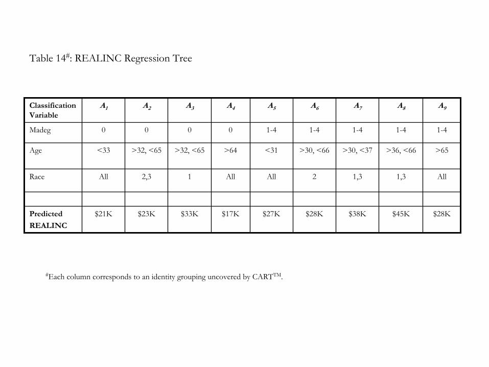
Table 14#: REALINC Regression Tree

$28K$45K$38K$28K$27K$17K$33K$23K$21KPredicted

REALINC

All1,31,32AllAll12,3 AllRace

>65>36, <66>30, <37>30, <66<31>64>32, <65>32, <65<33Age

1-41-41-41-41-40000Madeg

A9A8A7A6A5A4A3A2A1Classification Variable

#Each column corresponds to an identity grouping uncovered by CARTTM.

Table 15#: EQWLTH Classification Tree (with REALINC as classification variable)

6, 7**6, 7*713611Predicted Classification

AllAllAllAll21AllAllSex

AllAllAllAll1-41-40AllMadeg

AllAll>38>38<39<39<39AllAge

>62249>34002 and <62250

>14170 and <34003

<14171<34003<34003<34003AllRealinc

11111112,3Race

A8A7A6A5A4A3A2A1Classification Variable

#Each column corresponds to an identity grouping uncovered by CARTTM.* There are two terminal nodes split by years: 1980, 84, 89, 90, 91, 96.**There are two terminal nodes split by age: less than 49 and over 48.

Table 16: Summary of Results

No heterogeneity or different variables

HeterogeneityNo Heterogeneity (?)Mobility Beliefs

Heterogeneity (some similar variables)

At least as much het. as for Redist. Pref.

At least as much het. as for Redist. Pref.

Socioeconomic Status

Heterogeneity (different variables)

No HeterogeneityHeterogeneityTolerance for Inequality

HeterogeneityHeterogeneityHeterogeneityRedistribution Preference

ResultsPikettyBenabou & Ok

WORKING PAPER SERIES 2005 http://ase.tufts.edu/econ/papers/papers.html

2005-01 EGGLESTON, Karen, Keqin RAO and Jian WANG; “From Plan

to Market in the Health Sector? China's Experience.”

2005-02 SHIMSHACK Jay; “Are Mercury Advisories Effective?

Information, Education, and Fish Consumption.”

2005-03 KIM, Henry and Jinill KIM; “Welfare Effects of Tax Policy in

Open Economies: Stabilization and Cooperation.”

2005-04 KIM, Henry, Jinill KIM and Robert KOLLMANN; “Applying

Perturbation Methods to Incomplete Market Models with

Exogenous Borrowing Constraints.”

2005-05 KIM, Henry, Jinill KIM, Ernst SCHAUMBURG and Christopher

A. SIMS; “Calculating and Using Second Order Accurate

Solutions of Discrete Time Dynamic Equilibrium Models.”

2005-06 KIM, Henry, Soyoung KIM and Yunjong WANG; “International

Capital Flows and Boom-Bust Cycles in the Asia Pacific Region.”

2005-07 KIM, Henry, Soyoung KIM and Yunjong WANG; “Fear of

Floating in East Asia.”

2005-08 SCHMIDHEINY, Kurt; “How Fiscal Decentralization Flattens

Progressive Taxes.”

2005-09 SCHMIDHEINY, Kurt; “Segregation from Local Income Taxation

When Households Differ in Both Preferences and Incomes.”

2005-10 DURLAUF, Steven N., Andros KOURTELLOS, and Chih Ming

TAN; “How Robust Are the Linkages between Religiosity and

Economic Growth?”

2005-11 KEELY, Louise C. and Chih Ming TAN; “Understanding

Preferences For Income Redistribution.”

2005-12 TAN, Chih Ming; “No One True Path: Uncovering the Interplay

between Geography, Institutions, and Fractionalization in

Economic Development.”

2005-13 IOANNIDES, Yannis and Esteban ROSSI-HANSBERG; “Urban

Growth.”

2005-14 PATERSON, Robert W. and Jeffrey E. ZABEL; “The Effects of

Critical Habitat Designation on Housing Supply: An Analysis of

California Housing Construction Activity.”

2005-15 KEELY, Louise C. and Chih Ming TAN; “Understanding

Divergent Views on Redistribution Policy in the United States.”

2005-16 DOWNES, Tom and Shane GREENSTEIN; “Understanding Why

Universal Service Obligations May Be Unnecessary: The Private

Development of Local Internet Access Markets.”

2005-17 CALVO-ARMENGOL, Antoni and Yannis M. IOANNIDES;

“Social Networks in Labor Markets.”

2005-18 IOANNIDES, Yannis M.; “Random Graphs and Social Networks:

An Economics Perspective.”

2005-19 METCALF, Gilbert E.; “Tax Reform and Environmental

Taxation.”

2005-20 DURLAUF, Steven N., Andros KOURTELLOS, and Chih Ming

TAN; “Empirics of Growth and Development.”

2005-21 IOANNIDES, Yannis M. and Adriaan R. SOETEVENT; “Social

Networking and Individual Outcomes Beyond the Mean Field

Case.”

2005-22 CHISHOLM, Darlene and George NORMAN; “When to Exit a

Product: Evidence from the U.S. Motion-Pictures Exhibition

Market.”

2005-23 CHISHOLM, Darlene C., Margaret S. McMILLAN and George

NORMAN; “Product Differentiation and Film Programming

Choice: Do First-Run Movie Theatres Show the Same Films?”

2005-24 METCALF, Gilbert E. and Jongsang PARK; “A Comment on the

Role of Prices for Excludable Public Goods.”