Department of Economics

issn 1441-5429

Discussion paper 40/07

Unit Root Properties of Crude Oil Spot and Futures Prices

Svetlana Maslyuk1 and Russell Smyth2

ABSTRACT In this paper we examine whether WTI and Brent crude oil spot and futures prices (at one, three and

six months to maturity) contain a unit root with one and two structural breaks, employing weekly

data over the period 1991-2004. To realize this objective we employ Lagrange Multiplier (LM) unit

root tests with one and two endogenous structural breaks proposed by Lee and Stazicich (2003,

2004). We find that each of the oil price series can be characterized as a random walk process and

that the endogenous structural breaks are significant and meaningful in terms of events that have

impacted on world oil markets.

KEYWORDS Crude oil prices, Unit root, Stationarity

1 Department of Economics, Monash University, Vic, Australia Email: Svetlana.Maslyuk@buseco.monash.edu.au 2 Department of Economics, Monash University, 900 Dandenong Road, Caulfield East, Vic 3145, Australia Email: Russell.Smyth@buseco.monash.edu.au © 2007 Svetlana Maslyuk and Russell Smyth All rights reserved. No part of this paper may be reproduced in any form, or stored in a retrieval system, without the prior written permission of the author.

1 Introduction

There is no uniform view about the trajectory of commodity prices, including crude oil, over time.

Some theorists advocate deterministic trend models with either an upward (Simon, 1985) or

downward (Singer, 1950; Grili and Yang, 1988) trend for commodity prices relative to industry

prices. In the former, a steady increase in commodity prices can be attributed to economic growth.

In the latter a downward trend in commodity prices is due to deterioration in the terms of trade of

commodities, higher total factor productivity in agriculture relative to industry (Jalali-Naini and

Asali, 2004) or a decrease in transportation cost. There is no clear-cut upward or downward trend

over time for oil prices. Instead, oil prices have exhibited cyclical behavior (Jalali-Naini and Asali,

2004, Pindyck, 1999, Zivot and Andrews, 1992, Radchenko, 2005) and local trends (Cashin and

McDermott, 2002). Throughout history, oil prices have been very volatile, changing their

trajectories and behavior with respect to the economic situation. For industrial commodities

including oil, the most volatile years were 1971 and 1989 (Cashin and McDermott, 2002). These

years are important because the frequency of price movements increased substantially after 1971

(Cashin and McDermott, 2002, p.22) and the amplitude of price swings increased after 1989. For

example, Cashin and McDermott (2002, p.22) found that although trends in prices were highly

volatile, “price variability completely dominates long-run trends”.

In addition, there is a very strong seasonal component, where oil prices are traditionally higher

during winter than during summer. Since the end of the 1990s oil prices have been steadily

increasing, reflecting rising demand for crude oil particularly from developing nations. However,

there is no dominant upward trend. Instead, oil prices exhibit large upward or downward swings

primarily caused by “fluctuations in demand, extraction costs, and reserves” (Pindyck, 1999, p.12).

Any upward shifts in demand for oil or a rise in extraction costs will cause the spot and futures

prices of oil to increase, and this might lead to a change in the slope of the price trajectories

(Pindyck, 1999). After such swings, prices appear to revert to their long-run mean value or long-run

marginal cost, which also appear to change over time. Moreover, “temporary price spikes …

account for a large part of the total variation of changes in spot prices” (Blanco and Soronow, 2001,

p.83).

The purpose of this study is to examine unit root behaviour of crude oil spot and futures prices

allowing for one and two structural breaks. Our analysis is based on weekly data for spot and

futures prices for two market crudes; namely, the US West Texas Intermediate (WTI) and the UK

Brent over the period January 1991 to December 2004. One might expect oil prices to be stationary

because of market dynamics, time lags between price changes and demand/supply imbalances

(Pindyck, 1999; Postali and Picchetti, 2006). As discussed further in the literature review below, the

previous studies that have found mean or trend reversion in crude oil prices have typically used

annual data over periods ranging from 50 years to 140 years. The value of such findings is limited

because the lifespan of investment in a crude oil or natural gas field is about three decades (Postali

and Picchetti, 2006). Thus, we examine whether crude oil prices have a unit root over a much

shorter period, employing higher frequency data (weekly data). To realize this objective we employ

Lagrange Multiplier (LM) unit root tests with one and two endogenous structural breaks proposed

by Lee and Stazicich (2003, 2004). Compared with Augmented Dickey-Fuller (ADF) type tests that

accommodate endogenous structural breaks, the LM unit root test with structural breaks has the

advantage that the breaks are incorporated under the null. The LM unit root test with one and two

structural breaks has only been applied to energy prices twice before and that was with annual data

over a much longer period of time.

This paper is structured as follows. The next section discusses the rationale for examining the

stationarity of crude oil prices. Section 3 presents a literature review of studies of unit root tests

applied to crude oil prices. Section 4 provides a methodological overview of the unit root tests that

we apply in this paper. Section 5 gives an overview of the data as well as containing a discussion of

the potential break points. Section 6 presents the results. The final section concludes with a

discussion of the implications of the findings, considers some of the limitations of the research and

provides suggestions for future research.

2 Why does stationarity of crude oil prices matter?

The stochastic properties of crude oil prices have important implications for forecasting. As

Pindyck (1999) pointed out, ideally we would like to be able to explain crude oil prices in structural

terms because it is movements in demand and supply, and the factors that determine demand and

supply, that cause prices to fluctuate. However, structural models are not very useful for long-run

forecasting because it is difficult to come up with forecasts for the explanatory variables in such

models, such as investment and production capacity and inventory levels, over long time horizons.

As a consequence, industry forecasts of crude oil prices typically assume prices grow in real terms

at some fixed rate. One possibility is that prices follow a random walk. Another possibility is that

prices revert to a trend line, which implies that shocks to oil prices are temporary. As Pindyck

(1999) noted, if oil prices are trend reverting this is consistent with crude oil being sold in a

competitive market where price reverts to long-run marginal cost, which changes only slowly.

The stochastic properties of crude oil prices also have important implications for firms making

investment decisions. The issue of whether it is preferable to model crude oil prices as a Geometric

Brownian Motion (or some other related random walk process) or mean or trend reverting process

is important because investments are irreversible and, as such, have option like characteristics.

Baker et al. (1998) and Dixit and Pindyck (1994) show that different models of the pricing process

carry important implications for investment and valuation decisions. Pindyck (1999, p.2) noted:

“Simple net present value [NPV] rules are based only on expected future prices – second moments

do not matter for NPV assessments of investment projects. But this is not true when investment

decisions involve real options, as is the case when the investment is irreversible. Then second

moments matter very much, so that an investment decision based on a mean reverting process could

turn out to be quite different from one based on a random walk”. Research to evaluate oil and gas

deposits has developed complex multifactor models. However, as Postali and Picchetti (2006) have

stressed, if Geometric Brownian Motion is a reasonable proxy for the behavior of crude oil prices, it

is possible to find closed form solutions to a wide class of problems on real options without

complex numerical procedures.

Examining whether crude oil spot and futures prices contain a unit root has important implications

for investors. If crude oil spot and futures prices contain a random walk, it follows that the crude oil

market is efficient in the weak form, meaning future prices cannot be predicted using historical

price data. This implies that an uninformed investor with a diversified portfolio will, on average,

obtain a rate of return as good as an expert. If the random walk hypothesis is rejected it follows that

it is possible for investors to make profits using technical analysis. Rejection of the random walk

null hypothesis, based on a unit root with structural breaks does not necessarily imply that crude oil

spot and futures markets are inefficient or that crude oil spot and futures prices are rational

assessments of fundamental values. However, such a result would highlight the important role that

structural breaks can play in tests for unit roots and raise the important question of whether such

trend breaks should be treated like any other, or differently, before crude oil spot and future prices

are treated as either trend stationary or difference stationary (Serletis, 1992).

Finally, several studies have tested for a unit root in energy consumption or production (see eg.

Chen and Lee, 2007; Hsu et al., 2007; Narayan et al., 2007; Narayan and Smyth, 2007). These

studies emphasize that if energy consumption or production is non-stationary, given the importance

of energy to other sectors in the economy, other key macroeconomic variables would inherit that

non-stationarity. As Hendry and Juselius (2000) note, “variables related to the level of any variables

with a stochastic trend will inherit that non-stationarity, and transmit it to other variables in turn ….

Links between variables will then ‘spread’ such non-stationarities throughout the economy”. This

issue is just as pertinent for crude oil prices as crude oil consumption or production. Studies have

linked shocks to crude oil prices to output and inflation (Hamilton, 1996; Cunado and Perez de

Gracia, 2003), the natural rate of unemployment (Caruth et. al., 1998), movements in stock market

indices (Sardosky 1999; Papapetrou 2001) and fluctuations in business cycles (Kim and Loungani,

1992). From an economic viewpoint, if these macroeconomic series are non-stationary, business

cycle theories, which describe fluctuations in output as temporary deviations from the long-run

growth path will lose their empirical support.

3 Existing studies

It is common in the literature to explore the stochastic properties of crude oil prices prior to other

econometric analysis. Papers that have applied conventional unit root tests such as the ADF (Dickey

and Fuller, 1979) and Phillips and Perron (1988) (PP) tests and the KPSS (Kwiatkowski et al.,

1992) stationarity test to WTI and Brent crude oil prices include Sivapulle and Moosa (1999),

Serletis and Rangel-Ruiz (2004) and Taback (2003) among others. For example, Sivapulle and

Moosa (1999) apply the ADF, PP and KPSS unit root tests to daily WTI spot and one, three, and six

months to maturity WTI futures contracts covering the period January 2, 1985 to July 11, 1996.

They found all four variables to be non-stationary based on these traditional tests. Serletis and

Rangel-Ruiz (2004) applied ADF and PP tests to daily spot WTI crude oil prices from January 1991

to April 2001. They could not reject the unit root null. Taback (2003) tested whether Brent spot and

one, two and three months to maturity futures prices contain a unit root for the period January 1990

to December 2000 using the ADF test and found that both spot prices and futures prices for one-

and two-month contracts were non-stationary. Coimbra and Esteves (2004) tested the stationarity of

Brent crude oil spot and futures prices by applying the ADF test to oil prices for the period January

1989 to December 2003 as well as to a shorter period, which omitted the Gulf war, from January

1992 to December 2003. For both timeframes the null hypothesis of a unit root in crude oil prices

could not be rejected.

Studies that have tested for a unit root in the prices of crude oils other than WTI and Brent include

Alizadeh and Nomikos (2002) and Ewing and Harter (2000) among others. Alizadeh and Nomikos

(2002) tested for a unit root in weekly closing prices of WTI, Brent and Nigerian Bonny Light from

January 1, 1993 to August 10, 2001. They applied ADF, PP and KPSS tests and could not reject the

unit root null hypothesis. Using monthly data from 1974 to 1996, Ewing and Harter (2000) studied

co-movement of Alaskan and UK Brent crude oil prices. Based on the PP unit root test, they could

not reject the null of a unit root in either Alaskan or UK Brent crude oil prices. A recent

development in the literature has been to analyse the long-run properties of crude oil prices based

on unit root tests applied to long spans of data. Studies of this kind include Pindyck (1999) and

Krichene (2002), both of which employ annual aggregated data. Pindyck (1999) studied the long-

run evolution of American crude oil prices employing 127 years of annual data, from 1870 to 1996.

Krichene (2002) examined the time series properties of natural gas and crude oil production and

prices from 1918 to 1999. Both Pindyck (1999) and Krichene (2002) could not reject the unit root

null for these time periods with standard ADF tests.

There are not many studies of oil prices that have applied unit root tests that allow for either

exogenous or endogenous structural breaks. Gulen (1997) applied Perron’s (1989) ADF-type unit

root test with one exogenous structural break to spot and contract prices for US and non-US crudes

of different gravity. He selected February 1986 as the exogenous structural break because it

corresponded to the largest drop in oil prices over the entire sample period. He found that two of

the fifteen spot price series and three of the thirteen contract price series were stationary at the 5%

level of significance. In a second study Gulen (1998) applied Perron’s (1989) ADF-type unit root

test to New York Mercantile Exchange (NYMEX) monthly crude oil futures at one, three and six

months to maturity from March 1983 to October 1995 and treated February 1986 as the exogenous

break point. He was unable to reject the unit root hypothesis for any of the oil price series.

Serletis (1992) published the first study that tested for a unit root in oil prices with a single

endogenous structural break. He first applied the ADF and PP tests, then proceeded to apply the

Zivot and Andrews (1992) ADF-type unit root test with one endogenous structural break to a

sample of daily NYMEX energy futures prices, including crude oil, heating oil and unleaded

gasoline, over the period July 1983 to July 1990. Based on the ADF and PP tests he concluded that

all series contained a unit root. However, the Zivot and Andrews (1992) test rejected the unit root

null for all energy prices. Sadorsky (1999) applied the PP and Zivot and Andrews (1992) tests to

US monthly real oil prices measured using the producer price index for fuels. The period studied

spanned January 1947 to April 1996. Real oil prices were found to have a positive upward trend.

The unit root null hypothesis was rejected in favour of trend stationarity by both tests.

Lee et al. (2006) and Postali and Picchetti (2006) are recent studies of the unit root properties of

crude oil prices that have allowed for two endogeneous structural breaks. Lee et al. (2006) applied

the Lee and Stazicich (2003, 2004) LM unit root tests with one and two endogenous structural

breaks to eleven real commodity prices, including crude oil, from 1870 to 1990. They tested two

specifications: a unit root test with linear trend and a unit toot test with a quadratic trend. With a

linear trend and two endogenous breaks, they were able to reject the null of a unit root for all eleven

natural resource price series including petroleum. The two breaks were found to occur in 1896 and

1971, which corresponded to the end of the economic depression in the US and the termination of

the Gold Standard for the American dollar. However, with the quadratic trend in the two-break

model, the unit root null could only be rejected for five of the eleven series excluding petroleum.

The structural breaks were found to be in 1914 and 1926, which corresponded to the start of the

First World War and the General Strike in Great Britain respectively.

Postali and Picchetti (2006) also applied the Lee and Stazicich (2003, 2004) LM unit root tests with

one and two endogenous structural breaks to international oil prices. Similar to Pyndaik (1999),

Postali and Picchetti (2006) found that with annual data the length of the sample period was the

most important factor in determining whether the series had at least one unit root. They divided the

sample that covered 1861 to 1999 into several sub-samples spanning 50 years to 110 years.

Traditional ADF and PP tests were only able to reject the unit root null for the entire sample with

more than a century of annual data. For the sub-periods, conventional tests and LM unit root tests

with two breaks in the intercept could not reject the unit root null. However, allowing for two

breaks in the intercept and trend the unit root null hypothesis could be rejected for the period 1861-

1999 and the sub-periods.

In summary, stationarity of crude oil prices has not been confirmed by the majority of studies. The

failure of many of these studies to find that oil prices are mean-reverting processes might reflect the

low power of conventional unit root tests. These tests are typically criticized for their low power in

rejecting the alternative hypothesis of stationarity in small samples as noted by Pindyck (1999). In

addition, conventional tests give ambiguous results when the data is described by a near unit root

process or when the data is of high frequency with fat tails and volatility clustering (Boswijk and

Klaassen, 2005), which is a characteristic of crude oil prices. Moreover, results of these tests

crucially depend on the choice of lag in the model as well as the data frequency. Studies that have

found evidence of stationarity in crude oil prices have typically applied ADF-type or LM unit root

tests with structural breaks to annual data spanning 50 to 140 years.

4. Econometric methodology Unit root tests without structural breaks

In order to provide a benchmark for the LM unit root tests we begin through applying the ADF and

PP unit root tests. The ADF unit root test is based on the auxiliary regression:

t

k

jjtjtt ydtyy εωακ +Δ+++=Δ ∑

=−−

11 (1)

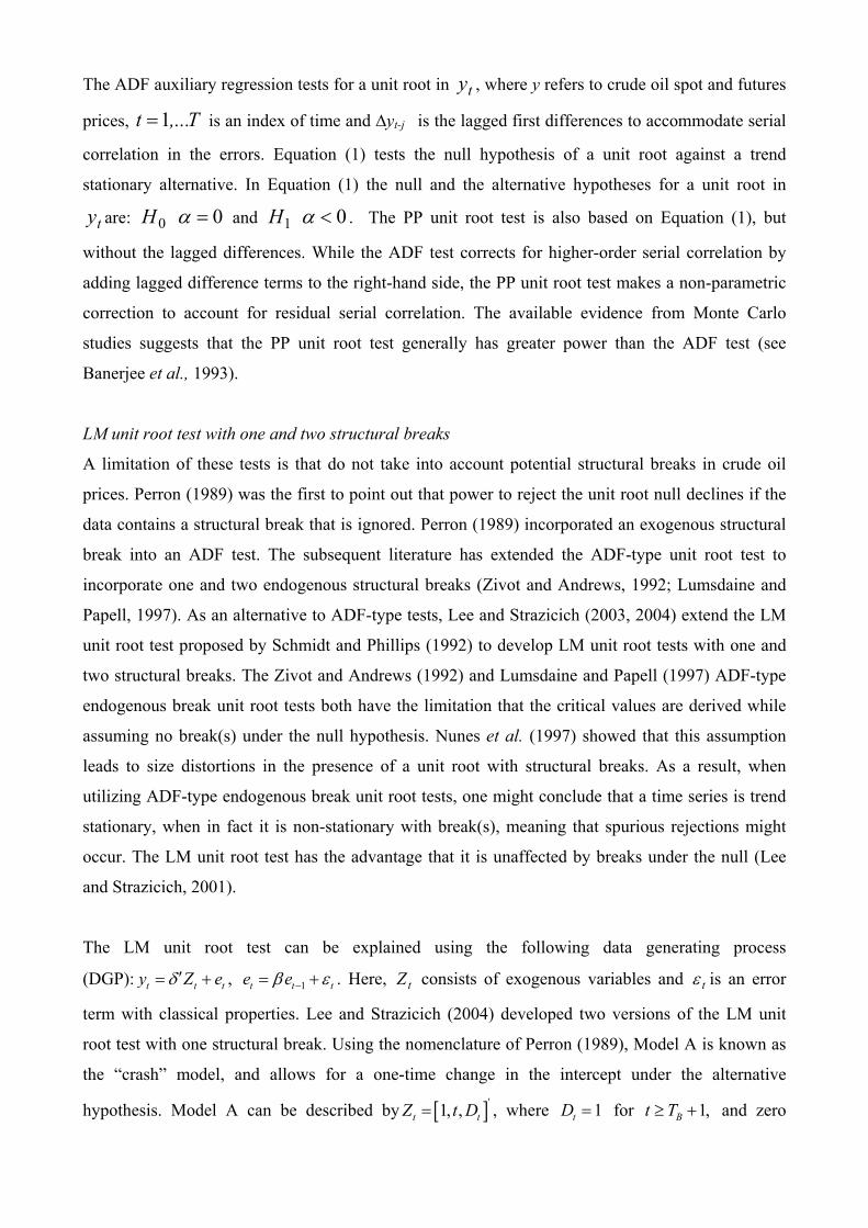
The ADF auxiliary regression tests for a unit root in ty , where y refers to crude oil spot and futures

prices, T,...t 1= is an index of time and ∆yt-j is the lagged first differences to accommodate serial

correlation in the errors. Equation (1) tests the null hypothesis of a unit root against a trend

stationary alternative. In Equation (1) the null and the alternative hypotheses for a unit root in

ty are: 0H 0=α and 1H 0<α . The PP unit root test is also based on Equation (1), but

without the lagged differences. While the ADF test corrects for higher-order serial correlation by

adding lagged difference terms to the right-hand side, the PP unit root test makes a non-parametric

correction to account for residual serial correlation. The available evidence from Monte Carlo

studies suggests that the PP unit root test generally has greater power than the ADF test (see

Banerjee et al., 1993).

LM unit root test with one and two structural breaks

A limitation of these tests is that do not take into account potential structural breaks in crude oil

prices. Perron (1989) was the first to point out that power to reject the unit root null declines if the

data contains a structural break that is ignored. Perron (1989) incorporated an exogenous structural

break into an ADF test. The subsequent literature has extended the ADF-type unit root test to

incorporate one and two endogenous structural breaks (Zivot and Andrews, 1992; Lumsdaine and

Papell, 1997). As an alternative to ADF-type tests, Lee and Strazicich (2003, 2004) extend the LM

unit root test proposed by Schmidt and Phillips (1992) to develop LM unit root tests with one and

two structural breaks. The Zivot and Andrews (1992) and Lumsdaine and Papell (1997) ADF-type

endogenous break unit root tests both have the limitation that the critical values are derived while

assuming no break(s) under the null hypothesis. Nunes et al. (1997) showed that this assumption

leads to size distortions in the presence of a unit root with structural breaks. As a result, when

utilizing ADF-type endogenous break unit root tests, one might conclude that a time series is trend

stationary, when in fact it is non-stationary with break(s), meaning that spurious rejections might

occur. The LM unit root test has the advantage that it is unaffected by breaks under the null (Lee

and Strazicich, 2001).

The LM unit root test can be explained using the following data generating process

(DGP): t t ty Z eδ ′= + , 1t t te eβ ε−= + . Here, tZ consists of exogenous variables and tε is an error

term with classical properties. Lee and Strazicich (2004) developed two versions of the LM unit

root test with one structural break. Using the nomenclature of Perron (1989), Model A is known as

the “crash” model, and allows for a one-time change in the intercept under the alternative

hypothesis. Model A can be described by [ ]'1, ,t tZ t D= , where 1tD = for 1,Bt T≥ + and zero

otherwise, TB is the date of the structural break, and δ' = (δ1 , δ2 , δ3). Model C, the “crash-cum-

growth” model, allows for a shift in the intercept and a change in the trend slope under the

alternative hypothesis and can be described by [ ]'1, , ,t t tZ t D DT= , where t BDT t T= − for 1,Bt T≥ +

and zero otherwise.

Lee and Strazicich (2003) developed a version of the LM unit root test to accommodate two

structural breaks. The endogenous two-break LM unit root test can be considered as follows. Model

AA, as an extension of Model A, allows for two shifts in the intercept and is described by

[ ]'1 21, , ,t t tZ t D D= where 1jtD = for 1, 1,2,Bjt T j≥ + = and 0 otherwise. BjT denotes the date when

the breaks occur. Note that the DGP includes breaks under the null (β= 1) and alternative (β< 1)

hypothesis in a consistent manner. In Model AA, depending on the value of β, we have the

following null and alternative hypotheses:

0 0 1 1 2 2 1 1: ,t t t t tH y d B d B y vμ −= + + + +

1 1 1 2 2 2: ,A t t t tH y t d D d D vμ γ= + + + +

where 1tv and 2tv are stationary error terms; 1jtB = for 1, 1,2,Bjt T j= + = and 0 otherwise. Model

CC, as an extension of Model C, includes two changes in the intercept and the slope and is

described by [ ]'1 2 1 21, , , , ,t t t t tZ t D D DT DT= , where jt BjDT t T= − for 1, 1,2,Bjt T j≥ + = and 0

otherwise. For Model CC we have the following hypotheses:

0 0 1 1 2 2 3 1 4 2 1 1: ,t t t t t t tH y d B d B d D d D y vμ −= + + + + + +

1 1 1 2 2 3 1 4 2 2: ,A t t t t t tH y t d D d D d DT d DT vμ γ= + + + + + +

where 1tv and 2tv are stationary error terms; 1jtB = for 1, 1,2,Bjt T j= + = and 0 otherwise. The LM

unit root test statistic is obtained from the following regression:

tttt SZy μφΔδΔ ++′= −1

where ttxttˆZˆyS δψ −−= , T,...,t 2= ; δ̂ are coefficients in the regression of tyΔ on tZΔ ; xψ̂ is

given by δtt Zy − ; and 1y and 1Z represent the first observations of ty and tZ respectively. The

LM test statistic is given by: =τ t-statistic for testing the unit root null hypothesis that 0=φ . The

location of the structural break ( )BT is determined by selecting all possible break points for the

minimum t-statistic as follows:

( ) ( )λτλτλ

~fln~Inf i = , where TTB=λ .

The search is carried out over the trimming region (0.15T, 0.85T), where T is the sample size. We

determined the breaks where the endogenous two-break LM t-test statistic is at a minimum. Critical

values for the one break case are tabulated in Lee and Strazicich (2004), while critical values for the

two break case are from Lee and Strazicich (2003).

5 Data and potential structural breaks

We use weekly spot and futures prices at one, three and six months to maturity for the two

benchmark crudes over the period spanning January 1991 to December 2004. We chose the US

WTI and the UK Brent as the representative crudes for this analysis since these two crudes have

well-established spot and futures markets. WTI futures are traded on the NYMEX and Brent futures

are traded on the Intercontinental Exchange (ICE). Wednesday prices were chosen to extrapolate

the day of the week effect. If the market was closed on Wednesday, the price of the previous trading

day was used. The source for the spot prices is the Energy Information Administration (EIA), while

futures prices were taken from NYMEX and ICE. Notice that for all of the series WTI was priced

higher than Brent.

INSERT FIGURES 1-4

Inspection of Figures 1-4 for spot prices and futures prices at one, three and six months to maturity

suggest that there is no dominating upward or downward trend throughout the whole sample period.

Instead, oil prices can be characterised by a small number of structural breaks and a large number of

jumps. But over the whole sample period, both the duration and the length of jumps changed. From

January 1991 to November 1998 there were small shocks that affected the mean value of prices, but

prices returned to the mean value with different speeds of adjustment. Over the period, November

1998 to December 2004, the behaviour of oil prices drastically changed and became more volatile.

During this timeframe, oil prices were governed by cycles of local upward and downward trends

initiated by a particular shock. The duration of these cycles substantially differs from time to time

and is dependent on the nature of the shock. More adverse shocks caused longer cycles. Moreover,

the downward shocks were generally more abrupt than the upward shocks, which in turn were more

cumulative. An example of the abrupt downward movement in both spot and futures was a big drop

in price on September 17, 2001 when the New York Stock Exchange and the NYMEX reopened

after September 11, 2001 for the first time. An example of a series of cumulative upward

movements was an increase in prices from May 2003 until prices reached a peak in December 2003.

This implies that in the oil market it is possible to have one large shock (such as the first or second

Gulf war) as well as a series of combined smaller shocks that change the trajectory of prices.

Similar conclusions can be drawn from an examination of futures prices at all maturities. That is,

futures prices for the two different crudes and different months to maturity respond to shocks in the

same manner. Moreover, futures respond to the same shocks as spot prices. Based on Figures 1-4 it

can be seen that both spot and futures prices are very volatile and are characterised by large jumps,

particularly in the later time period of the sample. If there was a large jump in the spot market, this

immediately translated into a jump in the futures market. There are no separate jumps that occur in

one market only. According to theories of price determination for storable commodities (see, eg.

Working, 1948, 1949; Telser 1958), such jump behaviour in crude oil prices can be largely

attributed to shocks in demand and supply and resulting demand/supply disequilibrium.

INSERT FIGURE 5

Figure 5 presents a crude oil market chronology, highlighting events that have impacted on oil

prices. The most drastic events in terms of their impact on oil prices have been the Asian financial

crisis and Russian default, which caused a large decrease in the price of oil, which combined with

increased OPEC production in 1998 “sent prices into a downward spiral” (Williams, 2005). Another

important event was the September 11, 2001 terrorist attack, which caused a sudden sharp decline

in both spot and futures oil prices. Political unrest in Venezuela in the first six months of 2002

caused an increase in oil prices. This was not a separate event, but a series of events in Venezuela

that kept oil markets in a perpetual state of unrest. The second Gulf War in March 2003 – caused an

immediate drop in oil prices. In the few months prior to the war, WTI and Brent futures prices

increased due to fears of market participants that Iraq’s oil pipelines and oil fields would be

destroyed in the first days of the war. However, this did not happen. The first Gulf War, on the

contrary, caused a long sharp upward swing in oil prices. Consistent with efficient market theory,

there is either no time lag or only a very small time lag in the market reaction to news. Thus, the oil

market is very sensitive not only to news, but also to the expectation of news. For example, prices

started increasing at the beginning of March 1999, several days before a meeting of oil-producing

countries. On March 23, 1999 OPEC and non-OPEC countries agreed to decrease the combined

production of crude oil which increased prices even further. Events that were connected to oil-

producing countries or the largest consumers of oil such as the US have had a greater impact on oil

prices than events unrelated to the oil market. For example, the strike in Venezuela affected oil

prices more than the outbreak of Severe Acute Respiratory Syndrome (SARS) in 2002.

6 Results

The results for the ADF and PP tests are reported in Table 1. We tested two specifications of the

ADF and PP tests. The first specification included a constant only and the second specification

included a constant and a time trend. Since the constant and time trend combination was significant

in each specification, this appears to be a better fit for the data. On the basis of the Modified Akaike

Information Criterion, the maximum lag was selected to be eight. For both the ADF and PP tests

and for each of the series the null hypothesis of a unit root cannot be rejected at the 5% level. These

results could be biased because of the failure to account for structural change in the data. Tables 2

and 3 present the results for the LM unit root test with a break in the intercept and a break in the

intercept and trend. We could not reject the unit root null for either model with any of the series.

INSERT TABLES 1-3

We now turn to examining the location of the break points. It is important to note that estimation of

an endogenous break point will not be precise and will not match a particular event date by date

(Christiano, 1992; Lee and Strazicich, 2001; Sen, 2003). Therefore, it is not possible to analyse the

speed of the reaction to the news in different markets based on the estimated break points. In Model

A each of the break points are statistically significant at the 10% level or better and for seven of the

eight series the breakpoint is statistically significant at the 1% level. In Model C the break in the

intercept is not statistically significant, while the break in the trend is statistically significant for

Brent spot, one-month Brent and six-month WTI at the 10% level or better. Model A and Model C

suggest different break dates. We would expect that the break point would be the same across the

series due to interconnection between spot and futures markets. While the choice of a break point

does not coincide within the series, oil prices respond to the same shocks, although with different

time lags. For Model A the breakpoint is the same for Brent spot, Brent one-month and Brent three-

months (November 8, 2000) and WTI spot, WTI one-month and WTI three-months (May 7, 2003).

The breakpoint for Brent six-months and WTI six-months lag their respective spot prices and

shorter maturities by one to two months. The breakpoints for Brent spot, Brent one-month, Brent

three-months and Brent six-months, follow a period between January 1999 and September 2000

during which oil prices tripled due to a cumulative effect of high world oil demand, OPEC oil

production cutbacks, a cold winter in the US and low oil stock levels. The breakpoint for WTI spot,

WTI one-month, WTI three-months and WTI six-months coincided with the second Gulf war, a

decision by the European Parliament to introduce an emissions trading scheme as well as Hurricane

Claudette which adversely affected Texan oil production in July 2003.

In Model C each of the break points occurred between November 1997 and September 1999. The

breaks at the end of 1997 and in 1998 could be a reflection of the Asian financial crisis and

consequent reduced demand for oil from Asia. The break in Brent spot, Brent one-month, WTI spot

and WTI one-month follow several relevant events in 1999. For example, in May 1999, the US

adopted a plan to reduce nitrogen oxides (NOx) emission levels from cars and light-duty trucks,

which also required refineries to reduce gasoline sulphur content and which affected standards for

refined oil imported to the US. In addition, in June 1999, Sudan started operating a pipeline linking

its Heglig oil field to Port Sudan on the Red Sea. The location of these break points also reflected

activity of the oil majors on the stock market. For instance, BP announced its plan to finalise a

merger with Amoco on July 16 and on July 18, Elf Aquitaine attempted a takeover of Total Fina.

INSERT TABLES 4 and 5

Tables 4 and 5 present the results for the LM unit root tests with two breaks in the intercept (Model

AA) and two breaks in the intercept and trend (Model CC). In both Models AA and CC, the null

hypothesis of a unit root with two structural breaks could not be rejected. In Model AA, at least one

of the breaks in the intercept is statistically significant. In Model CC the breaks in the intercept are

statistically insignificant, but the breaks in trend are statistically significant. In Model AA, the first

break for each of the series except one- and six-month Brent and six-month WTI futures occurred in

2000 and the second break occurred in 2003. The first break in the series could be due to a terrorist

attack on the US warship, Cole, in Yemen in October 2000. The second break could be a reaction to

the Gulf war in Iraq which started in March 2003. For one-month Brent the first break occurred in

2001 and the second break occurred in 2003. This can be seen as a reaction to what occurred in the

Brent spot market, where the difference between the second break in the spot market and the first

break in the one-month futures market is two weeks. Both breaks could be a reaction to December

and January events which involved problems with the natural gas market in the US. For six-month

Brent, both breaks occurred in 2001 and for six-month WTI both breaks occurred in 2003. For

three-month Brent only the first break was significant. In Model CC the first break for each series

occurs in 1999 and is associated with the same events as the one-break case, while the second break

occurs at the time of the terrorist attack on the World Trade Centre in New York.

7 Implications of findings and suggestions for further research

We have examined the stochastic properties of WTI and Brent crude oil spot and futures prices (at

one, three and six months to maturity), employing weekly data from 1991 to 2004. We have used

the LM unit root test with one and two breaks in the intercept (Models A and AA) and intercept and

trend (Models C and CC). The LM unit root test with structural breaks has the advantage over ADF-

type unit root tests with structural breaks that it is unaffected by breaks under the null. We find that

each of the oil price series can be characterized as a random walk process and that the endogenous

structural breaks are significant and meaningful in terms of events that have impacted on world oil

markets.

Some important policy implications emerge from our findings. First, for forecasting purposes, the

fact crude oil prices exhibit a random walk means that it is not possible to forecast future

movements in crude oil prices based on past behaviour, at least for the timeframe considered in this

study. The proviso is that studies such as Pindyck (1999) and Postali and Picchetti (2006) find

evidence of mean reversion over very long periods of time, although even in these cases the rate of

mean reversion is so slow that for the purposes of making investment decisions one could just as

equally treat the crude oil price as a Geometric Brownian Motion or related random walk process.

As Pindyck (1999, p.25) concluded, based on analysis of data spanning more than a century: “These

numbers suggest that for irreversible investment decisions for which energy prices are the key

stochastic variable, the Geometric Brownian Motion assumption is unlikely to lead to large errors in

the optimal investment rule”. Our results suggest this is particularly true for shorter periods of time,

even after allowing for structural breaks in crude oil prices.

Second, our findings provide support for the integrity of much of the literature on real options,

which assumes that input costs, output prices and other pertinent stochastic state variables follow a

geometric Brownian motion (Pindyck, 1999). Our results, together with studies employing data

over long periods that find at best slow mean reversion, suggest that Geometric Brownian Motion

assumption will not lead to meaningful undervaluation or overvaluation. If Geometric Brownian

Motion is a good proxy for movements in crude oil prices, modellers can take advantage of its

operational friendliness, effectively sidestepping the complexities of complex structural models

(Postali and Picchetti, 2006).

Third, our findings that oil spot markets and oil futures markets are efficient in the weak form mean

that future spot and futures prices cannot be predicted based on past prices. If futures markets are

efficient and participants have full information, the futures market will allocate the investment to

the most efficient outcome and individual investors with a diversified portfolio can invest with

confidence. This, in turn, suggests that institutional and regulatory mechanisms will not be as

important, compared with the situation where price movements could be exploited to make profits

using technical analysis.

Fourth, the fact that oil prices exhibit a random walk suggests that other macroeconomic variables

that are linked to oil prices via flow-on effects such as income and output will potentially inherit

that non-stationarity and transmit it to major economic variables such as employment. If non-

stationarity in oil prices spread to the real economy, this questions empirical support for business

cycle theories and a range of macro theories. As Cochrane (1994, p. 241) notes, lack of mean

reversion in real output “challenges a broad spectrum of macroeconomic theories designed to

produce and understand transitory fluctuations”.

A limitation on the results here is, as Lumsdaine and Papell (1997, p. 218) note, “we have little

reason to expect that there have been exactly two structural breaks [in the series considered]. In

addition our results do not address the possibility that even higher order models are more

appropriate. This begs the question of where to go next – to a model with three breaks?” There are

at least two possibilities which future research on the stochastic properties of oil prices could

follow. One avenue of inquiry would be to apply unit root tests with more than two breaks. Ohara

(1999) has developed an ADF-type unit root test with multiple structural breaks, while Westerlund

(2006) has developed an LM unit root test with multiple structural breaks. We note, though, the

more breaks which are added to the model, the closer the crude oil price series will be to a random

walk and the less relevant are unit roots with structural breaks (see Mehl, 2000, p. 376).

If regime-wise stationarity could be established allowing for further structural breaks or using data

over much longer periods, for which previous studies have found mean reversion, a second avenue

of research would be to test for the presence of multiple structural breaks using the method

proposed by Bai and Perron (1998). The Bai and Perron (1998) method can be applied to test for,

and estimate, multiple structural changes once regime-wise stationarity has been established. This

could be extended, using the approach pioneered by Caporale and Grier (2000) to examine political

influences on interest rates, to investigate the factors that explain oil price shocks. This could

contribute to the recent literature modelling oil price shocks (see eg. Kilian, 2005a, 2005b, 2007).

References Alizadeh, A.H., and Nomikos, N.K. 2002. Cost of carry, causality and arbitrage between oil futures and tanker freight markets. Paper presented at the IAME 2002 conference. Bai, J. and P., Perron 1998. Estimating and testing linear models with multiple structural changes. Econometrica, 66, 47-78. Baker, M.P., Mayfield, E.S. and Parsons, J.E. 1998. Alternative models of uncertain commodity prices for use with modern asset pricing methods. Energy Journal, 19, 115-148. Banerjee, A., Dolado, J.J., Galbraith, W. and Hendry, D.F. 1993. Cointegration, Error Correction and the Econometric Analysis of Non-stationary Data (Oxford: Oxford University Press). Blanco, C., and Soronow, D. 2001. Jump diffusion processes - energy price processes used for derivatives pricing and risk management. Commodities Now, 10, pp. 83-85. Boswijk, P.H., and Klaassen, F. 2005. Why frequency matters for unit root testing, Discussion Paper #04-119/4, Tinbergen Institute. Caporale, T. and K. Grier 2000. Political regime change and the real interest rate. Journal of Money, Credit and Banking, 32, 320-334. Caruth, A.A., Hooker, M.A. and Oswald, A.J. 1998. Unemployment equilibria and input prices: theory and evidence from the United States. Review of Economics and Statistics, 80, 621-28. Cashin, P., & McDermott, J.C. 2002. The long-run behaviour of commodity prices: small trends and big variability. International Monetary Fund Staff Papers, 49, 175-199. Chen, P.F. and Lee, C-C. 2007. Is energy consumption per capita broken stationary? New evidence from regional based panels. Energy Policy, 35, 3526-3540. Christiano, L.J. 1992. Searching for a break in GNP, Journal of Business and Economic Statistics, 10, 237-250. Cochrane, J.H. 1994. Permanent ant transitory components of GNP and stock prices, Quarterly Journal of Economics, 109, 241-266. Coimbra, C., and Esteves, P.S. 2004. Oil price assumptions in macroeconomic forecasts: should we follow futures market expectations? OPEC Review, 28, 87-106. Cunado, J. and Perez de Gracia, F. 2003. Do oil price shocks matter? Evidence for some European countries. Energy Economics, 25, 137-154. Dickey, D.A., and Fuller, W.A. 1979. Distribution of estimators for autoregressive time series with a unit root. Journal of American Statistical Association, 84, 427-431. Dickey, D.A., & Fuller, W.A. 1981. Likelihood ratio statistics for autoregressive time series with a unit root. Econometrica, 49, 1057-1072. Dixit, A. and Pindyck, R. 1994. Investment under uncertainty. Princeton, Princeton University Press. EIA 2006. Annual oil market chronology.

http://www.eia.doe.gov/emeu/cabs/AOMC/Overview.html (last accessed March 21, 2006). Ewing, B.T., and Harter, C.L. 2000. Co-movements of Alaska North Slope and UK Brent crude oil prices. Applied Economics Letters, 7, 553-558. Grilli, E., and Yang, M.C. 1988. Primary commodity prices, manufactured goods prices and the terms of trade of developing countries: what the long run shows. World Bank Economic Review, 2, 1-47. Gulen, G.S. 1997. Regionalization in the world crude oil market. Energy Journal, 18, 109-126. Gulen, G.S. 1998. Efficiency in the crude oil futures market. Journal of Energy Finance and Development, 3, 13-21. Hamilton, J.D. 1996. This is what happened to the oil-macroeconomy relationship. Journal of Monetary Economics, 38, 215-220. Hendry, D.F. and Juselius, K. 2000. Explaining cointegration analysis, part 1. Energy Journal, 21, 1-42. Hsu, Y.C., Lee, C-C. and Lee, C-C. 2007. Revisited: Are shocks to energy consumption permanent or stationary? New evidence from a panel SURADF approach. Energy Economics (in press). Jalali-Naini, A.R., and Asali, M. 2004. Cyclical behaviour and shock-persistence: crude oil prices. OPEC Review, 28, 107-131. Kilian, L. 2005. The effects of exogenous oil supply shocks on output and inflation: evidence from the G7 countries. C.E.P.R. Discussion Paper 5404. Kilian, L. 2005a. Exogenous oil supply shocks: how big are they and how much do they matter for the U.S. economy? C.E.P.R. Discussion Paper 5131. Kilian, L. 2007. Not all oil price shocks are alike: disentangling demand and supply shocks in the crude oil market, mimeo. Available at http://www.personal.umich.edu/~lkilian/oil3_052107.pdf Kim, L. and Loungani, P. 1992. The role of energy in real business cycle models. Journal of Monetary Economics, 29, 173-189 Krichene, N. 2002. World crude oil and natural gas: a demand and supply model. Energy Economics, 24, 557-576. Kwiatkowski, D., Phillips, P.C.B., Schmidt, P., and Shin, Y. 1992. Testing the null hypothesis of stationarity against the alternative of a unit root. Journal of Econometrics, 54, 159-178. Lee, J., and Strazicich, M.C. 2001. Break point estimation and spurious rejections with endogenous unit root tests. Oxford Bulletin of Economics and Statistics. 63, 535-558. Lee, J., and Strazicich, M.C. 2003. Minimum lagrange multiplier unit root test with two structural breaks. Review of Economics and Statistics, 85, 1082-1089. Lee, J., and Strazicich, M.C. 2004. Minimum LM unit root test with one structural break, Working Paper #04-17, Department of Economics, Appalachian State University.

Lee, J., List, J.A., and Strazicich, M.C. 2006. Non-renewable resource prices: deterministic or stochastic trends? Journal of Environmental Economics and Management, 51, 354-370. Lumsdaine, R.L., and Papell, D.H. 1997. Multiple trend breaks and the unit root hypothesis. Review of Economics and Statistics, 79, 212-218. Mehl, A. 2000. Unit root tests with double trend breaks and the 1990s recession in Japan. Japan and the World Economy, 12, 363-379. Narayan, P.K., Narayan. S. and Smyth, R. 2007. Are oil shocks permanent or temporary? Panel data evidence from crude oil and NGL production in 60 Countries. Energy Economics (in press). Narayan, P.K. and Smyth, R. 2007. Are shocks to energy consumption permanent or temporary? Evidence From 182 Countries. Energy Policy, 35, 333-341. Nunes, L., Newbold, P., and Kaun, C. 1997. Testing for unit roots with structural breaks: evidence on the great crash and the unit root hypothesis reconsidered. Oxford Bulletin of Economics and Statistics, 59, 435-448. Ohara, H.I, 1999. A unit root with multiple trend breaks: a theory and an application to US and Japanese macroeconomic time series. Japanese Economic Review, 50, 266-290. Papapetrou, E. 2001. Oil price shocks, stock market, economic activity and employment in Greece. Energy Economics, 23, 511-532. Perron, P. 1989. The great crash, the oil price shock and the unit root hypothesis. Econometrica, 57, 1361-1401. Phillips, P.C.B. and Perron, P. 1988. Testing for a unit root in a time series regression. Biometrika, 75, 335-46. Pindyck, R.S. 1999. The long-run evolution of energy prices. Energy Journal, 20, 1-27. Postali, F., and Picchetti, P. 2006. Geometric Brownian Motion and structural breaks in oil Prices: a quantitative analysis. Energy Economics, 28, 506-522. Radchenko, S. 2005. The long-run forecasting of energy prices using the model of shifting trend, Working Paper, University of North Carolina. Sadorsky, P. 1999. Oil price shocks and stock market activity. Energy Economics, 5, 449-469. Schmidt, P., and Phillips, P.C.B. 1992. LM test for a unit root in the presence of deterministic trends. Oxford Bulletin of Economics and Statistics, 54, 257-287. Sen, A. 2003. On unit root tests when the alternative is a trend-break stationary process. Journal of Business and Economic Statistics, 21, 174-185. Serletis, A. 1992. Unit root behaviour in energy futures prices. Energy Journal, 13, 119-128. Serletis, A., and Rangel-Ruiz, R. 2004. Testing for common features in North American energy markets. Energy Economics, 26, 401-414.

Simon, J.L. 1985. Forecasting the long-term trend of raw material availability. International Journal of Forecasting, 1, 85-93. Singer, H.W. 1950. The distribution of gains between investing and borrowing countries. American Economic Review, 40, 472-485. Sivapulle, P., and Moosa, I.A. 1999. The relationship between spot and futures prices: evidence from the crude oil market. Journal of Futures Markets, 19, 175-193. Taback, B.M. 2003. On the information content of oil future prices, Working Paper # 65, Banco Central de Brazil. Telser, L.G. 1958. Futures trading and the storage of cotton and wheat. Journal of Political Economy, 66, 233-255. Westerlund, J. 2006. Simple unit root tests with structural breaks. Mimeo, University of Lund. Williams, J., 2005. Oil price history and analysis, WTRG economics http://www.wtrg.com/prices.htm (last accessed May 24, 2006). Working, H. 1948. Theory of the inverse carrying charge in futures markets. Journal of Farm Economics, 30, 1-28. Working, H. 1949. The theory of price of storage. American Economic Review, 39, 1254-1262. Zivot, E., and Andrews, D. 1992. Further evidence of the great crash, the Oil-price shock and the unit root hypothesis. Journal of Business and Economic Statistics, 11, 251-270.

Table 1 ADF and Phillips-Perron unit root tests for oil spot and futures prices

ADF unit root test Phillips-Perron unit root test Variable With

constant With constant

and trend With constant With

constant and trend

Brent Spot -1.7103 (0.4256)

-3.2992 (0.0671)

-1.3644 (0.6007)

-3.1090 (0.1049)

Brent 1 month -1.4217 (0.5727)

-3.0595 (0.117)

-1.2847 (0.6384)

-3.0468 (0.1203)

Brent 3 months -0.8063 (0.8163)

-2.4741 (0.3411)

-0.7728 (0.8256)

-2.4748 (0.3407)

Brent 6 months -0.2444 (0.9301)

-1.8765 (0.6657)

-0.2465 (0.9298)

-1.8835 (0.6621)

WTI Spot -1.3719 (0.5971)

-2.9221 (0.156)

-0.9812 (0.7615)

-2.6747 (0.2476)

WTI 1 month -1.3292 (0.6175)

-2.8818 (0.1691)

-0.9410 (0.7751)

-2.6093 (0.2762)

WTI 3 months -0.6973 (0.8452)

-2.3089 (0.4281)

-0.5731 (0.8737)

-2.2856 (0.4408)

WTI 6 months 0.0057 (0.9578)

-1.5724 (0.8031)

0.0572 (0.9622)

-1.5457 (0.813)

Note: p-values for the ADF and Phillips-Perron statistics are given in parentheses.

Table 2 LM unit root test results for Model A

Variable Lag order TB Bt LM test statistic Brent Spot 7 November 8, 2000 2.4073**

(2.1951) -1.8959

Brent 1 month 7 November 8, 2000 2.2698** (2.2762)

-1.7924

Brent 3 months 7 November 8, 2000 1.7886** (2.1651)

-1.7673

Brent 6 months 7 January 31, 2001 2.2906*** (3.2881)

-1.5882

WTI Spot 7 May 7, 2003 2.6236*** (2.3244)

-1.8851

WTI 1 month 7 May 7, 2003 2.7499*** (2.5212)

-1.8619

WTI 3 months 7 May 7, 2003 1.9549** (2.1659)

-1.5657

WTI 6 months 6 June 11, 2003 1.3865* (1.8179)

-2.4359

Note: TB is the date of the structural break; B(t) is the dummy variable for the structural break in the intercept. Figures in parentheses are t-values. Critical values for the LM test statistic from Lee and Strazicich (2004) at the 10%, 5% and 1% significance levels are -3.211, -3.566, -4.239. Critical values for the dummy variables follow the standard normal distribution. * (**) *** denote statistical significance at the 10%, 5% and 1% levels respectively.

Table 3 LM unit root test results for Model C

Lag order TB B(t) D(t) LM test statistic Brent Spot 7 August 11, 1999 0.2978

(0.2739) 0.2310*** (2.3242)

-2.9267

Brent 1 month 7 September 1, 1999 1.2228 (1.2359)

0.1815** (2.0943)

-2.8382

Brent 3 months 7 December 17, 1997 -0.0010 (-0.0012)

0.0333 (0.5425)

-2.9244

Brent 6 months 7 December 17, 1997 0.0689 (0.0993)

-0.0039 (-0.0703)

-2.9149

WTI Spot 7 September 8, 1999 1.6925 (1.5019)

0.1428 (1.5939)

-2.7890

WTI 1 month 7 September 8, 1999 1.6459 (1.5115)

0.1390 (1.6078)

-2.7563

WTI 3 months 7 November 12, 1997 -0.0538 (-0.0597)

0.0009 (0.0127)

-2.6929

WTI 6 months 5 August 19, 1998 0.9389 (1.2344)

-0.1461* (-1.8732)

-3.9825

Note: TB is the date of the structural break; B(t) is the dummy variable for the structural break in the intercept; D(t) is the dummy variable for the structural break in the slope. Figures in parentheses are t-values. The critical values for the LM test statistic depend on the location of the break and are as follows:

Location of break, λ 0.1 0.2 0.3 0.4 0.5 1% significance level -5.11 -5.07 -5.15 -5.05 -5.11 5% significance level -4.50 -4.47 -4.45 -4.50 -4.51 10% significance level -4.21 -4.20 -4.18 -4.18 -4.17

Critical values for the dummy variables follow the standard normal distribution. * (**) *** denote statistical significance at the 10%, 5% and 1% levels respectively.

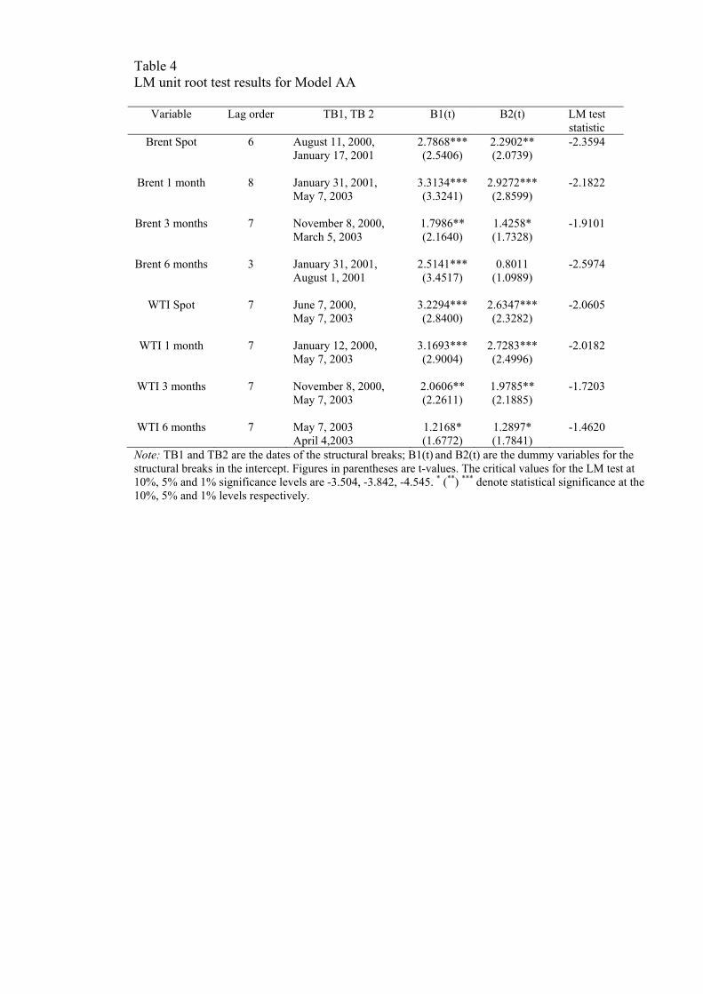
Table 4 LM unit root test results for Model AA

Variable Lag order TB1, TB 2 B1(t) B2(t) LM test statistic

Brent Spot 6 August 11, 2000, January 17, 2001

2.7868*** (2.5406)

2.2902** (2.0739)

-2.3594

Brent 1 month 8 January 31, 2001, May 7, 2003

3.3134*** (3.3241)

2.9272*** (2.8599)

-2.1822

Brent 3 months 7 November 8, 2000, March 5, 2003

1.7986** (2.1640)

1.4258* (1.7328)

-1.9101

Brent 6 months 3 January 31, 2001, August 1, 2001

2.5141*** (3.4517)

0.8011 (1.0989)

-2.5974

WTI Spot 7 June 7, 2000, May 7, 2003

3.2294*** (2.8400)

2.6347*** (2.3282)

-2.0605

WTI 1 month 7 January 12, 2000, May 7, 2003

3.1693*** (2.9004)

2.7283*** (2.4996)

-2.0182

WTI 3 months 7 November 8, 2000, May 7, 2003

2.0606** (2.2611)

1.9785** (2.1885)

-1.7203

WTI 6 months 7 May 7, 2003 April 4,2003

1.2168* (1.6772)

1.2897* (1.7841)

-1.4620

Note: TB1 and TB2 are the dates of the structural breaks; B1(t) and B2(t) are the dummy variables for the structural breaks in the intercept. Figures in parentheses are t-values. The critical values for the LM test at 10%, 5% and 1% significance levels are -3.504, -3.842, -4.545. * (**) *** denote statistical significance at the 10%, 5% and 1% levels respectively.

Table 5 LM unit root test results for Model CC

Variable Lag order Estimated break points B1(t) B2(t) D1(t) D2(t) LM test statistic

Brent Spot 7 July 14, 1999, October 17, 2001

-1.3955 (-1.2682)

0.5614 (0.5053)

0.7869*** (3.6798)

-0.3297** (-2.0278)

-4.1142

Brent 1 month 7 August 18, 1999, October 17, 2001

-1.0787 (-1.0786)

0.4057 (0.4032)

0.6784*** (3.4413)

-0.2781* (-1.8362)

-3.9326

Brent 3 months 7 July 14, 1999, October 17, 2001

-0.8504 (-1.0265)

0.4815 (0.5756)

0.5209*** (3.5296)

-0.2697** (-2.0707)

-4.0647

Brent 6 months 7 July 14, 1999, October 17, 2001

-0.9322 (-1.3289)

0.3589 (0.5070)

0.3929*** (3.3622)

-0.2396** (-2.0714)

-3.9364

WTI Spot 7 August 18, 1999, September 26, 2001

-1.2064 (-1.0603)

-0.4311 (-0.3775)

0.7504*** (3.4973)

-0.3754** (-2.0854)

-4.0370

WTI 1 month 7 August 18, 1999, September 26, 2001

-1.2495 (-1.1371)

-0.5862 (-0.5306)

0.7269*** (3.4881)

-0.3593** (-2.0573)

-4.0080

WTI 3 months 7 July 14,1999, October 17, 2001

-0.9045 (-0.9951)

0.4416 (0.4807)

0.5502*** (3.4294)

-0.3139** (-2.1055)

-3.9462

WTI 6 months 7 May 26,1999, October 17, 2001

-0.6523 (-0.9006)

0.2174 (0.2957)

0.3606*** (3.3122)

-0.2918** (-2.2736)

-3.7592

Notes: TB1 and TB2 are the dates of the structural breaks; B1(t) and B2(t) are the dummy variables for the structural breaks in the intercept; D1(t) and D2(t)are the dummy variables for the structural breaks in the trend. Figures in parentheses are t-values. For model CC, critical values depend on the location of the breaks and are as follows: Critical values for St-1

Λ2 0.4 0.6 0.8 Λ1 1% 5% 10% 1% 5% 10% 1% 5% 10% 0.2 -6.16 -5.59 -5.27 -6.41 -5.74 -5.32 -6.33 -5.71 -5.33 0.4 - - - -6.45 -5.67 -5.31 -6.42 -5.65 -5.32 0.6 - - - - - - -6.32 -5.73 -5.32 λj denotes the location of breaks. * (**) *** denote statistical significance at the 10%, 5% and 1% levels respectively.

0

10

20

30

40

50

60

1992 1994 1996 1998 2000 2002 2004

BRENT WTI

Pric

es (U

S d

olla

rs)

Figure 1

Spot Brent and WTI: weekly prices

0

10

20

30

40

50

60

1992 1994 1996 1998 2000 2002 2004

BRENT1 WTI1

Pric

es (U

S d

olla

rs)

Figure 2

1 month to maturity Brent and WTI weekly futures prices

10

20

30

40

50

60

1992 1994 1996 1998 2000 2002 2004

BRENT3 WTI3

Pric

es (U

S d

olla

rs)

Figure 3:

3 months to maturity Brent and WTI weekly futures prices

10

20

30

40

50

60

1992 1994 1996 1998 2000 2002 2004

BRENT6 WTI6

Pric

es (U

S d

olla

rs)

Figure 4:

6 months to maturity Brent and WTI weekly futures prices

Figure 5 Crude oil market chronology: January 1991 to December 2004

0

10

20

30

40

50

60

1/01

/199

1

1/07

/199

1

1/01

/199

2

1/07

/199

2

1/01

/199

3

1/07

/199

3

1/01

/199

4

1/07

/199

4

1/01

/199

5

1/07

/199

5

1/01

/199

6

1/07

/199

6

1/01

/199

7

1/07

/199

7

1/01

/199

8

1/07

/199

8

1/01

/199

9

1/07

/199

9

1/01

/200

0

1/07

/200

0

1/01

/200

1

1/07

/200

1

1/01

/200

2

1/07

/200

2

1/01

/200

3

1/07

/200

3

1/01

/200

4

1/07

/200

4

pric

e, U

SD

Iraq starts import of oil under UN 986 resolution

President Clinton authorised sale of 30 mln bbl of oil from the Strategic Petroleum Reserve (SPR)

Asian crisis, oil oversupply

Between January 1999 and September 2000 prices tripled due to high world oil demand, OPEC oil production cutbacks, cold winter in US and low oil stock levels.

Last Kuwait fire is extinguished

UN threatens sanctions against Lybia

OPEC's supply reaches 10 year max 25.3 mln b/d

OPEC increased oil price

Cold winter in US and EU

U.N. Resolution 986 was accepted. Also, President Clinton authorised sale of 227 mln bbl of oil from the Strategic Petroleum Reserve (SPR)

Nigerian worker's strike

September 11, 2001

Second Iraq war

Prices increased because of low capacity, political instability.

Source: based on the EIA (2006) Annual Oil Market Chronology