VICTORIA ~

U.NWERSll 0 ..

DEPARTMENT OF COMPUTER AND MATHEMATICAL SCIENCES

Summation of Series of Binomial Variation

A. Sofo and P. Cerone

86MATH 13

April, 1997

(AMS: 05Al5, 05A19, 39Al0)

TECHNICAL REPORT

VICTORIA UNIVERSITY OF TECHNOLOGY P 0BOX14428

J\1ELBOURNE CITY MC VIC 8001 AUSTRALIA

TELEPHONE (03) 9688 4492 FACSIMILE (03) 9688 4050

F ootscray Campus

~SE.R.BV

Summation of Series

of Binomial Variation

A. SOFO and P. CERONE

Department of Computer and Mathematical Sciences

Victoria University of Technology Australia

April, 1997

2

Abstract

Difference delay and discrete renewal equations provide a rich source of material for the

exploration and generation of infinite series. From this vantage point it will be shown that,

with certain restrictions, these generated infinite series may be represented in closed form.

The analysis will consist of an application of the Z transform together with a detailed

description of the location of zeros of polynomial type characteristic functions.

Introduction

In this paper a technique is developed that allows for the exploration and generation of infinite

series which in turn may be represented in closed form. Renewal processes provide a rich

source of material for such investigations and of critical importance in our work, is the form of

the characteristic equation in the denominator of a queue-length generating function including

the location of zeros.

In section 1, a discrete renewal equation will be considered and a method developed for the

generation of Binomial type infinite series, by considering a similar characteristic function as

produced by a bulk service queue. To analyse the discrete renewal equation a generating

function approach by the use of the Z transform will be employed. It will be shown that the

infinite series may be represented in closed form such that the closed form representation may

be expressed in terms of the dominant zero of a characteristic function.

For a particular parameter values of the series, the closed form identity may be confirmed by

the WZ pairs method ofWilf and Zeilberger [11].

Section 2 investigates the connection of the Binomial type series with generalized

hypergeometric functions. For a particular case the Binomial series will be shown to satisfy

the identity of Kummer [7].

In section 3 we consider a modified density function in the discrete renewal equation.

The closed form representation of the generated series may then be expressed in terms of a

multiple number of dominant zeros of an associated characteristic function. In section 4, we

consider a forcing term in the difference-delay representation of the stationary size

probabilities, that yields an interesting Binomial convolution identity.

3

1. A Volterra Type Discrete Renewal Equation

The analysis is begun by considering a volterra type discrete renewal equation

71

fn == Wn + Lfn-k <J>k (1.1) k=O

where fn may represent the total average number of r:enewals at epoch n , $11

may

represent the probability that a new item that is installed at a given time will fail after

exactly n time units and w11

may represent the average number of renewals at time n

of the original population. For a derivation of (1.1) one can refer to the books of

Saaty [12] or Cohen [5].

Alternatively (1.1) may be represented as, where *is the discrete convolution

' !

(1.2)

Therefore by the use of the Z transform (1.2) may be written as, after rearrangement

F(z) == W(z) 1-<l>(z)

(1.3)

where F(z), W(z) and <l>(z) are the Z transforms of the respective functions f,,, w11

and <l>n·

4

Without loss of generality a convolution type argument of (1.3) will allow for the

consideration of the more general transform function,

F z)- W(z) ( - (1-<1>(z)Y

(1.4)

for R = 1, 2, 3, 4,...... .

A Bulk Service Queue

The simplest Markovian queue to which the characteristic functions in the

denominator of (1.4) becomes germane is the bulk service variation of the MIM(a)II

system in which service is in fixed batches of size 'a', irrespective of whether or not the

server has to wait for a full batch of size a, see Gross and Harris [9].

To obtain a similar characteristic function as that of the MIM(a)ll system, consider the

densities

:: ( n )bn-(R-1) R-1 wn R-l c and

<l>n = bn-a U(n-(a+ 1))

where U(n - x) is the discrete step function, a 2:: 1, c E 9\, b e9\ and R 2:: 1.

Let W(z) and <l>(z) be the Z transform of (1.5) and (1.6) respectively, then

ZCR-1 W(z)= ( y

z-b

b -a

<l>(z) =-z­z-b

and

(1.5)

(1.6)

(1.7)

(l.8)

5

Substituting (1.7) and (1.8) into (1.4) yields, upon simplification, the transformed

function

1 ~~ R=I F;(z) = F(z) = ( z )" = ( )'. (1.9) c z-b-bz-a za+l _bza -b

An equivalent characteristic function as the denominator of (1.9) may be obtained

when the stationary system-size probabilities are related in difference - equation form.

It has been shown by Sofo and Cerone [14] that the same generating function (1.9) for

the case R = 1 can be arrived at via the use of a related Fibonacci sequence, see also

Kelley and Peterson [10].

Expanding the second term of (1.9) in series form results in

F(z) = ~ (R + r - l)br Zl-ar

,£..J r ( - b)r+R r=O Z

(1.10)

and therefore the inverse Z transform of (1.10) is

(1.11)

Equation (1.11) may also be rewritten as

[n+l-R] f. = ~ (R + r - l)(n -ar )bn-ar-{R-1) " £..J r R+r-1

r=O (1.12)

6

where [x] represents the integer part of x.

The inverse transform of (1.9) may also be expressed as, refer to Elaydi [6],

In=~ fcz"(F(z))dz = IResj(F(z))z" 21tl Z j=O Z

(l.13)

where C is a smooth Jordan curve enclosing the singularities of (1.9) and the integral

is traversed once in an anticlockwise direction around C. It may also be shown that

there is no contribution from the integration around the contour C. Re sj is the

residue of the poles of (1.9).

From (1.9), the characteristic function (with some restriction)

g(z) = za+l - bza -b (1.14)

has exactly (a+ 1) distinct zeros, sj for j = 0, 1, 2 ....... a' of which at least one and at

most two are real. See appendix B for a clarification of this statement.

Therefore s;+1 - bs; -b = 0, and all the singµlarities in (1.9) are poles of order R.

Now, from (1.9) , F(z) has exactly '(a+ 1)' poles of order R at the zeros Sr

Hence from (1.13) a solution of the system (1.2) may be expressed as

(l.15)

where the residue contribution

(l.16)

for each j =0, 1, 2, ....... a.

7

From (1.11) or (1.12) and using (1.15) it can be seen that

~(R + r-l)(n-ar )bn-ar+l-R U(n-ar) ~ r R+r-1

_ n n-(R-1-µ) a R~ ( ) - ~ ~Q-(R,-µ)(~j) R-1-µ ~j •

(1.17)

Main Result

The characteristic function (1.14) has at least one real zero. The dominant real zero,

~o of (1.14) is defined as the one with the greatest modulus, and it may be easily

shown that l~ol > 3:!!...._. Details of this statement are given in Appendix B. a+l

The limiting behaviour of (1.17) is such that for n large

[n+l-R]

a+l (R 1)( ) R-1 ( ) f, = ~ +r- n-ar bn-ar+I-R - ~ Q (~ ) n ~n-{R-I-µ) 0 n £..J r R+r-1 £..J -{R.-µ) 0 R-1-µ 0

r=O µ=O

(1.18)

The suggestive limiting behaviour of (1.18), leads the authors to the conjecture that

~(R+r-l)(n-ar )bn-ar+I-R = ~ Q (~ )( n )~n-{R-1-µ) £..J r R + r - l £..J '-<R.-µ) 0 R-1- µ 0 r=O µ=O

(l.19)

for all values of n (and not just n large) in the region where the infinite series converges.

The conjectured result (1.19) together with the equation (1.17) implies that

[ "~R] (R + r - I)(n -ar )bn-ar+l-R + ~ (R + r- I)(n- ar )b"-ar+l-R = ~ n , ( ~ )( n )~"-(R-1-µ) £.... r R+r-I £... r R+r-1 £..."'°'""\R.-µ) 0 R-1-µ 0 ~ [~] ~ r=-a+l

8

which gives the result

~ (R + r - l)(n -ar )bn-ar+l-R = _ ~ ~ n , _ ( ~ .)( n )~-{R-1-µ). £.J r R+r-1 £.. £..~R. µ) 1 R-1-µ 1

[n+2-R] j=l µ=O r=--

a+l

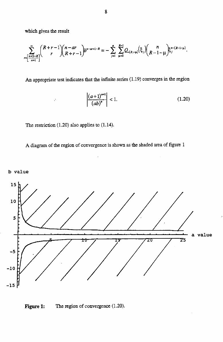
An appropriate test indicates that the infinite series (l.19) converges in the region

(a+ly+i ·~----1 <I.

(abY (1.20)

The restriction (l.20) also applies to (1.14).

A diagram of the region of convergence is shown as the shaded area of figure 1

b value

15

10

s

a value

-5

-10

-15

Figure 1: The region of convergence (l.20).

'

I

I

9

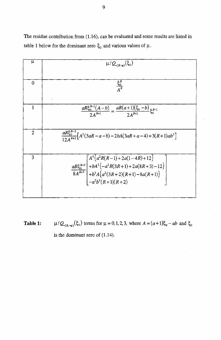
The residue contribution from (l.16), can be evaluated and some results are listed in

table 1 below for the dominant zero ~0 and various values of µ.

µ µf Q-(R-µ)(~o)

0 ~~ AR

aR~~-1 (A-b) = aR(a+l)(~0 -b) ~R-I 1 2A R+l 2AR+l 0

2 R~R-2 ~2A ~+2 [ A

2(3aR- a-8)-2bA(3aR+ a-4) + 3(R + l)ab2]

3 ,-A3{ a2R(R-l)+2a(l-4R)+ 12} -I

aR~~-3 +bA2{-a2R(3R+1) + 2a(8R + 3)-12} 8AR+3 +b2A{a2(3R+ 2)(R+ 1)-8a(R+ 1)}

'

-a2b3(R + l)(R+ 2) I

-

Table 1: µ!Q_(R.-µ)(~0 ) terms for µ=0,1,2,3, where A=(a+l)~0 -ab and ~o

is the dominant zero of ( 1.14 ).

'

10

Utilizing the terms of table 1 the closed form expressions of (1.19) are listed in table 2,

for various R values

R '

1

2

3

4

Table 2:

The closed form expression of (1.19)

~~+1

A

-n+ ~;·1 [ a(a+ 1)(~0 -b)]

A2 A

~;·1 [ ( n )+( n) 3a(A-b) + a(2(a-l)A

2 -(5a-2)bA +3ab

2)]

A3 2 1 2A 2A2

- (n)+(n)2a(A-b) +(nt((11a-8)A2-2b(13a-4)A+ 15ab

2r 3 2 A 1 6A2

I

~~+1 +~{A3(12a2 -30a+12)+bA2 (-52a2 +70a-12) A4 l2A

+b2A(10a2 -40a)-30a2b3}

-I

The closed form expressions of the infinite sum at (1.19) for the values

R = 1, 2, 3 and 4. Where A = (a+ 1 )~0 - ab and ~o is the dominant zero

of (l.14).

The proof of the conjecture at (1.19) can now proceed.

11

Proof of Conjecture

The proof of (1 .19) will involve the application of an induction argument. Firstly a

recurrence relation will be developed for the series

S = ~ (R + r - l)(n - ar )bn-ar+I-R. R ~ r R+r-1

(1.21)

Lemma

A recurrence relation for (l.21) is

d (a+l)b-S -abRS -(n+l-R)S =0 db R R+l R

(1.22)

Proof

.!!:._ 5 =-E.~ r(R+r-l)(n-ar )bn-ar-R+i+(n+l-R)s db R b ~ r R + r -1 b R

and

S = ~ (R + r)(n - ar)bn-ar-R R+I £.. r R+r

r=O

= _ (a+I)~r(R+r-l)(n-ar )bn-ar-R+I+(n+l-R)s bR ~ r R + r -1 bR R

From the left hand side of (1.22).

(a+l)b[(n+l-R)s _a~ r(R+r-l)(n-ar )bn-ar-R+I] b R b ~ r R+r-1

-abR[ (a+ 1) ~ r(R+r-l)(n-ar )bn-ar-R+I +(n+ 1-R)s ]-(n+ l-R)S bR ~ r R + r -1 bR R R

12

= 0 which is the right hand side of (l.22)

and the proof of the lemma in complete.

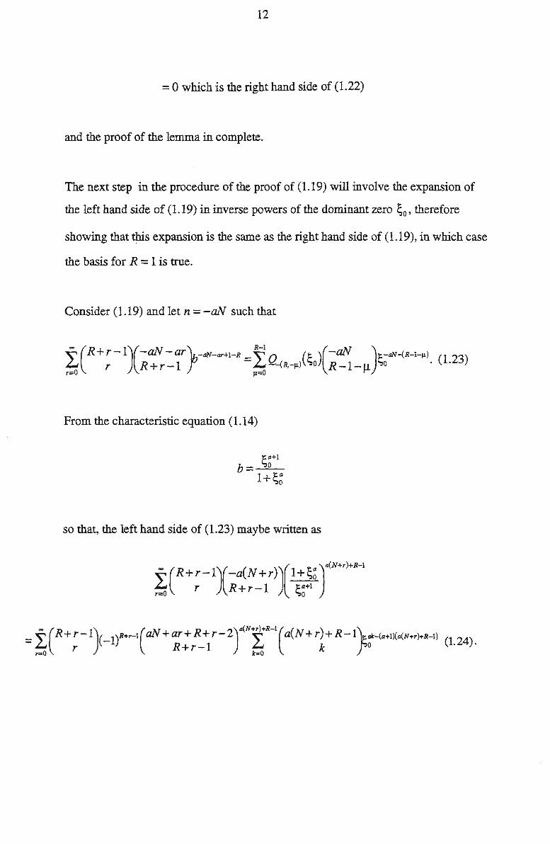
The next step in the procedure of the proof of (1.19) will involve the expansion of

the left hand side of (1.19) in inverse powers of the dominant zero So, therefore

showing that ¢is expansion is the same as the right hand side of (l.19), in which case

the basis for R = 1 is true.

Consider (1.19) and let n = -aN such that

~(R+r-1)(-aN-ar}-aN-ar+I-R = ~ Q (; )(-aN );-aN-(R-1-µ). (1.23) kt r R + r - l kt -(R,-µ) 0 R-1-µ 0 r=O µ=O

From the characteristic equation (1.14)

~a+l b=-0-

l+~~

so that, the left hand side of (1.23) maybe written as

~(R+ r-l)(-a(N + r))(l +~~ )a(N+r)+R-l kt r R + r -1 ~ a+1 r=O i.,o

13

The convergent double sum (1.24) may be written term by term as

(-l)R-1 (R- l)(aN + R- 2)[(aN + R-1)~-(a+IXaN+R-1) (aN + R-1)~-a(N+O)-(R-l)] 0 R -1 , 0 ~o +. · · · · · · · · · · · · · · · · · + aN + R -1 ~o

(-l)R(R)(aN +a+ R-l)[(aN +a+ R-1),i:-(a+l)(aN+a+R-1) (aN +a+ R-1),i:-a(N+l)-(R-1)] + 1 R 0 "=>o + ............. + aN+a+R-1 "=>o

( -l)R+l (R + 1)( aN + 2a + R)[( aN + 2a + R -1)~ -(a+l)(aN+2a+R-l) ( aN + 2a + R -1)~ -a(N+Z)-(R-I) J ( 1.25) + · 2 R + 1 0 '='0 + .. ··· ··· · ·· ·· + aN + 2a + R -1 '='0

(-l)R+2(R + 2)(aN + 3a + R- l)[(aN + 3a + R- l)i:;-(a+1)(aN+3a+R-1) (aN + 3a+ R- l)i:;-a(N+3)-(R-l)] + 3 R + 2 0 '='0 + .. · · ····· · ·· · + aN + 3a + R-1 '='0

+ ................................................................................................ .

Summing (1.25) diagonally from the top right hand comer and gathering the

coefficients of inverse powers of ~0 gives

~ ~-a(N+r)-(R-l)(-lt-t+r'f (-l)k(R+ r-k-l)(a(N + r-k)+ R+ r-k-2)(a(N + r-k)+ R-1 )· (l.Z6) £.J 0 £.J r-k R+r-k-1 a(N+r-k)+R-k-1 r=O k=O

In the case that R=l, (1.26) is again expanded to allow for the collection of the ~~ar

terms such that

~ ~-a(N+r)~ (-lY+k(a(N +r-k) )(a(N +r-k)+r-k-1) k 0 k a(N+r-k)-k r-k r=O k=O

~-aN[ 1+~~ ] 0 {a+l)+;~

14

= ;~aN+l

(a+ 1);0 -ab putting n = - aN gives

(1.27)

From the right hand side of (1.19) and using (1 .16) for R = 1

n n-(R-l-µ) ":lo R-l ( ) ~n+l

~Q-(R.-µ) (;o) R-1-µ o (a+l)~o-ab (1.28)

and comparing (1.27) and (1.28) indicates that (1.19) is proved for R = 1.

Now, we consider the right hand side of (1.19) for the general case R

S _ n n-(R-1-µ) R-l ( )

R - ~ Q-(R.-µ)(;o) R-1-µ o

and utilize the recurrence relation (1.22).

SR+i =-1-[(a+l)b!!_SR-(n+l-R)sRJ·

abR db (1.29)

. d ;~ d5 Firstly, from - SR = -b d~ R

db A ":lo I

d ;~ R-I ( n \n-{R-l-µ)[ d (n-(R-1 ~µ)) ] db SR = Ab ~ R -1-µf 0 d;

0 ~R.-µ) + ;o ~R,-µ)

15

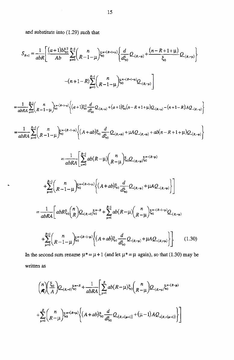
and substitute into (1.29) such that

S =-1-[(a+l)b~~~( n )~n-{R-l-µ){_!!_n . +(n-R+I+µ)Q_ } R+I abR Ab £... R - I - µ 0 dJ= ~R.-µ) J: (R.-µ )

µ=O ..,0 ..,0

-( n + l - R) ~ ( n )J:n-{R-1-µ)Q ] £..i R - I - µ ..,0 -(R,-µ) µ=O

In the second sum rename µ * = µ + 1 (and let µ * = µ again), so that (1.30) may be

written as

16

_ n n (n )i:n-R 1 f ( n \n-CR-µ)[ ( )!: - X:-Cl,--O)X:-CR.--0) R l:io + abRA f=t R - µ ro ab R-µ l:IOQ-(R.-µ)

_ n . (n )J:n-R 1 ~( n \n-(R-µ)[ b( )!: - X:-CR+l,--0) R ""o + abRA;::. R- µ ro a R - µ ..,OQ-(R.-µ)

+(A + ab) ~o d~, Q-( R,-{µ-1)) + (µ -1) A Q-( .. 1.-11) l (l.31)

Now utilizing the lemma in appendix. A, and after replacing µ with µ -1 we have

d abRAQ(R+l,-µ) = ab{R- µ)~O~R.-µ) +(A +ab)~o d~o Q-(R,-(µ-1)) +(µ- l)AQ_(R.-(µ-1))

so that, from (l.31) we have

n n~ n ~~~ ( )

R ( } R ~o ~R+1.--0) + ~ R _ µ o Q-(R+l.-µ)

_ n n-(R-µ ) R ( } - ~ R - µ 0 Q-(R+l,-µ)

which completes the proof of (1.19).

Some numerical results are now given for various parameter values of (1.19).

I

17

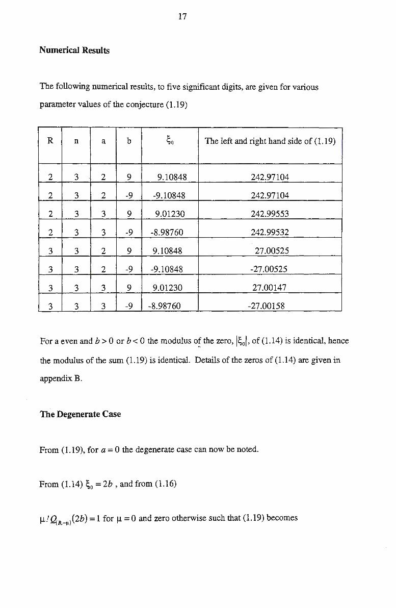
Numerical Results

The following numerical results, to five significant digits, are given for various

parameter values of the conjecture (1.19)

R n a b ~o The left and right hand side of (1.19)

2 3 2 I 9 9.10848 242.97104

2 3 2 -9 -9.10848 242.97104

2 3 3 9 9.01230 242.99553

2 3 3 -9 -8.98760 242.99532

3 3 2 9 9.10848 27.00525

3 3 2 -9 -9.10848 -27.00525

3 3 3 9 9.01230 27.00147

3 3 3 -9 -8.98760 -27.00158

I

For a even and b > 0 orb< 0 the modulus of the zero, !~0 j, of (1.14) is identical, hence

the modulus of the sum (l.19) is identical. Details of the zeros of (1.14) are given in

appendix B.

The Degenerate Case

From (1.19), for a= 0 the degenerate case can now be noted.

From (1.14) ~0 = 2b , and from (1.16)

µ!~R.-µ.)(2b) = l forµ =0 and zero otherwise such that (l.19) becomes

18

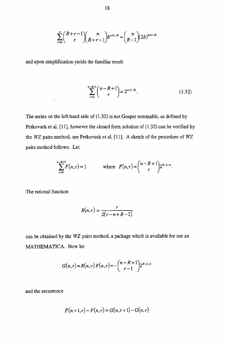
~(R+r-1)( n )bn+1-R =( n )(2br+1-R £... r R+r-l R-l r=O

and upon simplification yields the familiar result

n-R+1( R 1) L n - r + = 2n+l-R •

r=O (1.32)

The series on the left hand side of (1.32) is not Gosper summable, as defmed by

Petkovsek et al. [11], however the closed form solution of (l.32) can be verified by

the WZ pairs method, see Petkovsek et al. [ 11]. A sketch of the procedure of WZ

pairs method follows. Let

n-R+l

LF(n,r)=l r=O

h F( ) -(n -R + 1)2R-1-n w ere n,r - . r

The rational function

R(n,r) = r 2(r-n+R-2)

can be obtained by the WZ pairs method, a package which is available for use an

MATHEMATICA. Now let

and the recurrence

F(n + l,r )- F(n,r) = G(n,r+ l)-G(n,r)

19

including the initial condition F( O,r) = 1 holds, hence the identity (1.32) is verified.

In the next section we investigate the connection of the series (l.21) with generalised

hypergeometric functions.

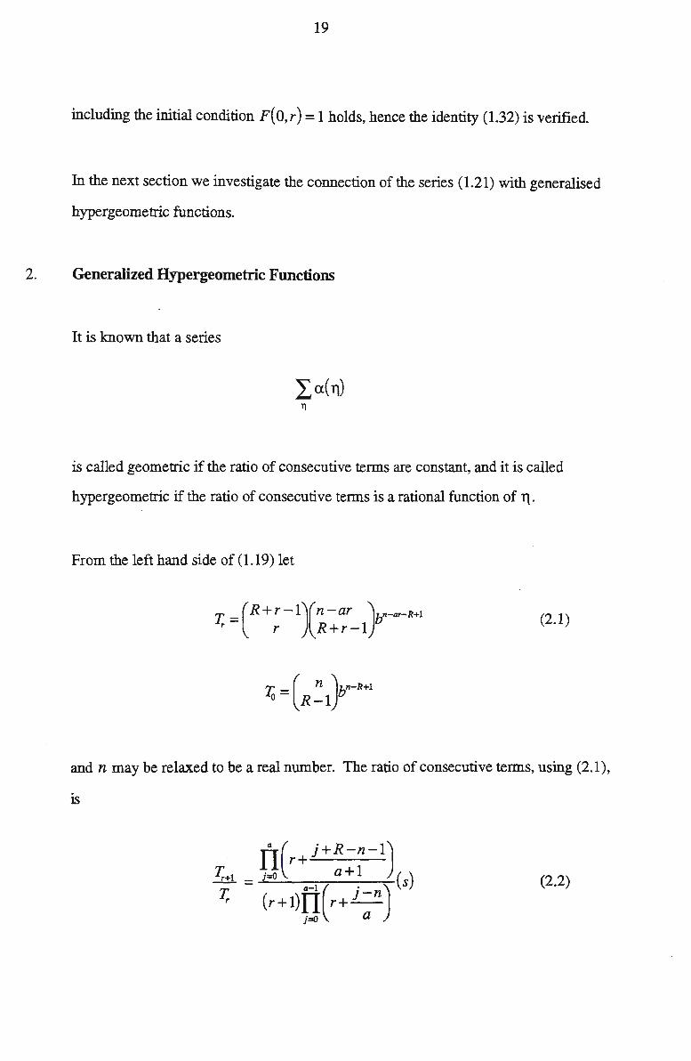
2. Generalized Hypergeometric Functions

It is known that a series

is called geometric if the ratio of consecutive terms are constant, and it is called

hypergeometric if the ratio of consecutive terms is a rational function of T\.

From the left hand side of (1.19) let

T. = (R + r - l)(n -ar )bn-ar-R+l r I r R+r-1

L = ( n )bn-R+l 0 R-1

(2.1)

and n may be relaxed to be a real number. The ratio of consecutive terms, using (2.1 ),

is

IT( j+R-n-lJ

T,+1 = j=O r ~-1 a + ~ ( s) T, (r+l)fi(r+ 1-nJ.

i=-O a

(2.2)

20

Since (2.2) is a quotient of rational functions in r, then the left hand side of (1.19) may

be expressed as a generalized hypergeometric function,

1 R-n-l R-n R-n+l R+a-n-l '

a+l ' a+l ' a+l , ........ ,

a+l Ta a+1F:i s (2.3)

n l-n 2-n a-1-n , ........ '

a a a a

00 (R-n-l) (R-n) (R-n+l) ···········(R+a-n-l) k -z::L a+l k a+l k a+l k a+l k s

-

0

•=' (-:). (1:n). (2:n ).. .......... ..(°-~-n). k! (Z.4)

where (x)m =x(x+ 1) ........... (x+m-l) is known as Pochhammer's symbol or as

rising factorial powers of m, as mentioned by Graham et al. [8], and

(a+1r+1

s = - (abt .

. ,

(2.5)

Generalizing the expression 15.1.1 given on page 556 of Abromowitz and Stegun [1],

allows (2.3) or (2.4) to be written as

a-1 ( • ) a+R-1 ( · ) fir 1-n 00 fir 1-n+k . k

T,., j=O a "" j=R-l a + 1 !.._ 0 a+R-1 ( • ) .£..t a-1 ( • ) k f II r 1-n k=O fir 1-n +k .

i=R-1 a+ 1 j=o a

(2.6)

where r( x) is the classical Gamma function. It is evident that (2.4) is a divergent

series for n a positive integer. Many relations of the generalized hypergeometric

function (2.3) exist in terms of the special functions of mathematical physics, and some

of these may be seen in the classical works of Slater [13] and Gaspar and Rahman [7].

21

Some special cases of (2.3) are worthy of mention, since for a= 1, (2.3) reduces to

the classical Gauss series. Thus letting a= 1 in (2.3), we have that

[

R - n -1 , R - n ( 4 )] To 2F'i 2 2 --

-n b . (2.7)

2t-l

_ [l(R-n-1+ j) = T,, 1 + """' j=O 0 k.--~-k--1~~~

t=I k!bk Il(n- j) j=O

The Gauss hypergeometric series (2.6) may be expressed as an integral. From

Abramowitz and Stegun, let ex.= -n e9\\J-, so that (2.7) may be written as

To f (l -t/a-R-2)12 /R+a-2)12(1- stil-R-«)12 dt (2.8) B( R +ex. ex. - R) r=o 2 , 2

which is valid for Isl < 1 , s = -4 lb and B( x, y) is the Beta function.

Since the difference in the two top terms of the hypergeometric function (2. 7) is V2,

there exists a quadratic transformation [13] connected with the Legendre functions,

P.,11• A definition of the Legendre function P: may be seen in [1]. From (2.7) and

using identity 15.4.11 of [1] we have that

4 whre s=-- and se(-oo,0).

b

22

Since the left hand side of (1.19) converges for b > 4, in the case that a= 1, then we

may write from (2.9) that

(2.10)

for b > 4 , "2~0 = b+.Jb2 +4b and Q-{R,-µ)(~0 ) is defined by (1.16).

Other specific cases of (2. 7) and (2.9) are as follows

(i) 3

For b = 4 , s = -1 and a= - , we have from (2.9) and 15.1.22 of [1], 2

Moreover, since the parameters in the hypergeometric function (2.11) gives the result

R +.!.-~-~+~ = 1 then the left hand side of (2.11) satisfies Kummer's identity [11], 2 4 2 4 2

= I:~R,-µ)(~o)( -~ J~~-R-~ 11=0 R-1-µ ·

R 1 R 3 -+- -+--T., R 2 4 ' 2 4 - l - 0 2 1 3

2

(2.12)

23

In equation (2.10), with b = 4 the characteristic function

g(z) =z2-4z-4

gives the dominant zero, ~o = 2(1+../2). Some values of (2.12) are

R=l R=2 I R=3 R=4 II

i I

1 -(2+../2) 3(2+../2) -5 1 l

s(1+.J2)2 1 1

.J247 (1 +.J2)2 2.43(1+../2)2 2../245(1 +.J2)2 I

I

(ii) Another elegant identity may be obtained from (2.10). Upon putting b = 4 and 1

a=-, we have that 2

R 1 R 1 --- -+-2 4'2 4_1

1 (2.13)

2

which may be extracted from identity 15.1.21 of Abramowitz and Stegun. We

may now conclude that, from (2.13) and (1.19)

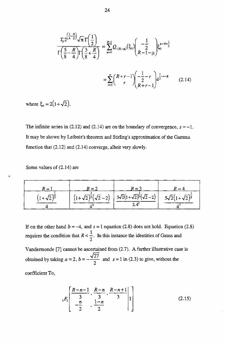
24

i)Hl~rG) - ,_, ( _.! J µ.-R+-i

.(5 R) (3 R) - LQ_(R,-11)(~0) 2 ~o r. --- r -+- . µ=0 R-1-µ 8 4 8 4

= f (R+;-1)(- ~ -r 14~-r-R (2.14) r=o R+r-1

where ~0 = 2( 1 + ../2).

The infinite series in (2.12) and (2.14) are on the boundary of convergence, s = -1.

It may be shown by Leibniz's theorem and Stirling's approximation of the Gamma

function that (2.12) and (2.14) converge, albeit very slowly.

Some values of (2.14) are

R=l R=2 R=3 R=4 I I 1 I

(1+.J2)2 ( 1 + .J2)2 ( .J2 - 2) 3.J2(1 +.J2)2(.J2-2) s.J2(1 +.J2)2

4 43 2.45 41

If on the other hand b = -4, ands= 1 equation (2.8) does not hold. Equation (2.8)

requires the . condition that R < _!_. In this instance the identities of Gauss and 2

V andermonde [7] cannot be ascertained from (2. 7). A further illustrative case is

obtained by talcing a= 2, b = - J27 and s = 1 in (2.3) to give, without the 2

coefficient To,

R-n-l R-n R-n+l --3£i 3 3 3 1 (2.15)

n 1-n -- --2 2

25

Following the preceeding argument relating to 2R, it may be stated that (1.19) diverges

and (2.15) will not yield the identities of Dixon, Saalschutz, Watson or Whipple, see

Gaspar and Rahman [7].

The result of equation (l.19) can now be extended by varying the form of the

characteristic function (1.14). In the next section the case of more than one dominant

zero of a characteristic function affecting the closed form solution of an associated

infinite series will be investigated. For this case a modified probability density function

will be considered in the application of a discrete renewal equation.

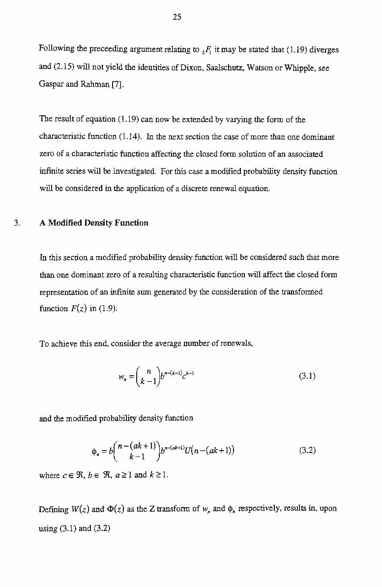
3. A Modified Density Function

In this section a modified probability density function will be considered such that more

than one dominant zero of a resulting characteristic function will affect the closed form

representation of an infinite sum generated by the consideration of the transformed

function F(z) in (1.9).

To achieve this end, consider the average number of renewals,

= ( n )bn-{k-1) k-1 wn k-1 c (3.1)

and the modified probability density function

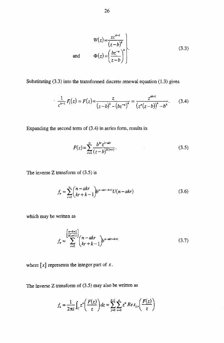
(3.2)

where c E 9\, b e 9\, a ~ 1 and k ~ 1.

Defining W(z) and <P(z) as the Z transform of wn and <l>n respectively, results in, upon

using (3.1) and (3.2)

and

26

k-1

W(z) ( zc y z-b

~(z)=(:~:J (3.3)

Substituting (3.3) into the transformed discrete renewal equation (1.3) gives

1 z z~I · k=I Fi(z) = F(z)= k ( k = ( t · (3.4)

c ( z - b) - bz -a) za ( z - b) - bk

Expanding the second term of (3.4) in series form, results in

oo bkr ZI-akr

F(z)= L ( -b)k(I+r) • r=O Z

(3.5)

The inverse Z transform of (3.5) is

+ = ~ (n -akr 1n-akr-k+1u( _ kr) Jn £.. kr+k-1 n a

r=O

(3.6)

which may be written as

[n-k+I]

k(a+I) ( ak } + = """' n - T n-akr-k+I Jn £.. kr+k-1

r=O

(3.7)

where [x] represents the integer part of x.

The inverse Z transform of (3.5) may also be written as

27

where Re sj,v is the residue of the poles of (3.5) and C is a smooth Jordan curve

enclosing the singularities of (3.5).

From (3.5), the characteristic function (with some restriction)

(3.8)

has exactly k(a+l) distinct zeros ~j.v for j=0,1,2, .. .. ,(k-1) and v=0,1,2, ... ..... ,a,

of which at least one and at most four are real. See appendix B for an explanation of

this statement.

Therefore ( ~~) ~j, v - b) r -bk = 0' and all the singularities in (3.4) are simple poles.

Hence from (3.4), F(z) has exactly k(a+ 1) simple poles, so that

k-1 a

1,, = IIQ(~j.J~;.v (3.9) j=O v=O

where the residue contribution

~j,v (3.10)

28

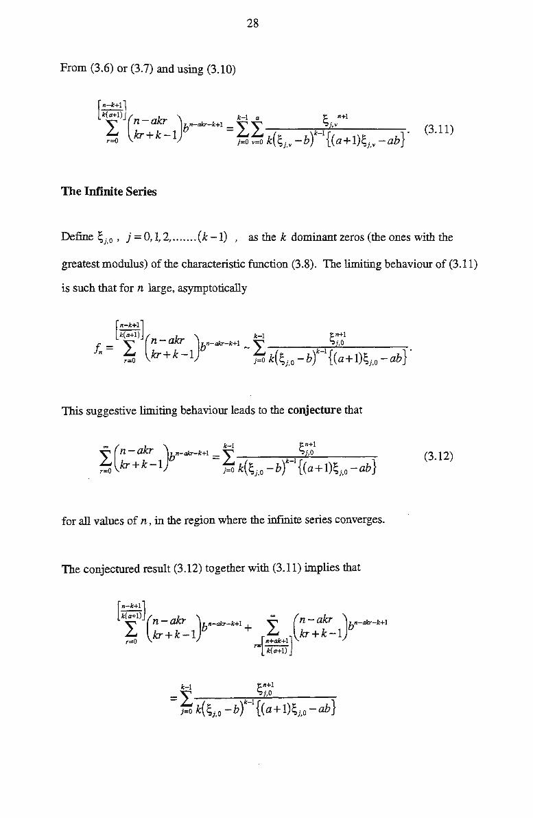
From (3.6) or (3.7) and using (3.10)

[n-k+l]

k(a+l) ( _ k ) k-1 a ):: n+l ~ n a r bn-akr-k+l = ~ ~ ~j.v £..i kr + k -1 £..i £..i k-1 • r=O j=O v=O k(~j.v -b) {(a+l)~j, v -ab}

(3.11)

The Infinite Series

Define ~j. o , j = 0, 1, 2, ....... (k-1) , as the k dominant zeros (the ones with the

greatest modulus) of the characteristic function (3.8). The limiting behaviour of (3.11)

is such that for n large, asymptotically

[n-k+l]

· k(a+l) ( ) k-1 J:;n+l

f, = ~ n-akr bn-akr-k+l _ ~ ~i.D •

n £..i kr + k - 1 £..i k-1 r=O j=ok(~j,0 -b) {(a+l)~j,0-ab}

This suggestive limiting behaviour leads to the conjecture that

(3.12)

for all values of n, in the region where the infinite series converges.

The conjectured result (3.12) together with (3.11) implies that

[n-k+l]

k(a+l) ( akr ) "" ( k ) """ n - bn-akr-k+I + """ n - a r bn-akr-k+I

(:t kr+k-1 r=[~+l] kr+k-1 k(a+l)

k-1 ~n+l -I j.o - j=O k( ~j,O -b t-l {(a+ l)~j,O -ab}

29

which gives that result

00

( k ) k-1 a J:n+I ~ n-a r bn-akr-k+I = _ ~ ~ '°'j.v

£.... kr+k 1 £....£.... k-I • J n+ak+I] - j=O v=I k( ~j.v -b) {(a+ l)~j. v -ab} ·-l .c(a+1)

Application of the ratio test indicates that the infinite series (3.12) converges in the region

{(a+It+I }k

(abY < 1

'

which is the same as (l.20), and this restriction also applies to equation (3.8).

Proof of result (3.12)

The characteristic function (3.8) may be expressed as the product of factors such that

k-I k-I

g(z) = { za(z-b)r -bk= Il(za+l -bza -be21tijlk) = 11 q/z) (3.13) j=O j=O

Now, consider each of the factors in (3.13) and write

za+I F(z)=----

1 a+I b a be21tijlk z - z -(3.14)

for each j = 0, 1, 2, ... .. (k -1).

The singularities in (3.14) with restriction (1.20) are all simple poles and therefore for

each j, Pj(z) has exactly '(a+l)' simplepolesofwhichai.o shall indicate the

dominant zero of each of the factors qi( ai.0 ) in (3.13).

30

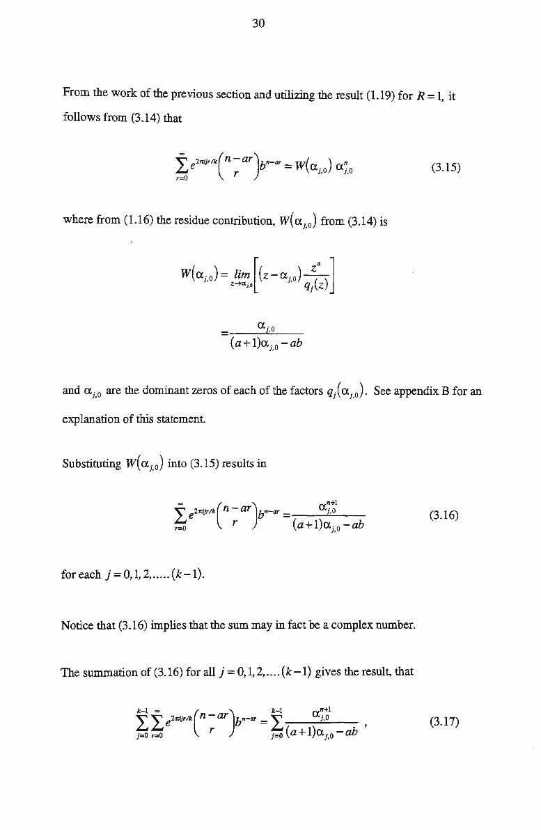
From the work of the previous section and utilizing the result (1.19) for R = 1, it

follows from (3.14) that

~ e2rtijrlk,(n - ar)bn-ar = w(a. . ) a.~ ~ r 1.o ,,o r=O

(3. 15)

where from (l.16) the residue contribution, w(a.i.0) from (3.14) is

w(a.j,0) = lim [(z-Uj,O) z(a )] z~ai.o qi Z

U j,O

(a+ l)aj,o -ab

and aj,o are the dominant zeros of each of the factors qi( aj,o). See appendix B for an

explanation of this statement

Substituting w(aj,o) into (3.15) results in

oo ( ) an+l L e21tijrlk n ~ ar bn-ar = j,O -r=O (a+ l)a.j,O ab

(3.16)

for each j=0,1,2, ..... (k-l).

Notice that (3.16) implies that the sum may in fact be a complex number.

The summation of (3.16) for all j = 0, 1, 2, .... ( k - l) gives the result, that

k-1 00 ( ) k-1 an+l ~ L e21tijrlk n ~ ar bn-ar = ~ j,O - ' ;=O r=O ;=O (a+ l)aj,O ab

(3.17)

31

Rescaling the left hand side of (3.17) by r = (r *+ l)k and then replacing r *by r

results in, after changing the order of summation

LL e21tij(r+l) n - a r + n-ak{r+l) = L Cl. j,O 00

k-1 ( k( 1)} k-1 n+l

r=-li=O k(r+ 1) i=O (a+ l)aj.o -ab

L n-a -a n-akr-ak = L aj,O - bn 00

( kr k} k-1 n+l

r=O . kr+k j=Ok{(a+l)et.j,0-ab} (3.18)

Now make the substitution n - ak = m in (3.18) such that

(3.19)

Newton's eh forward difference formula of a function h( xi) = hi at xi is defined as

(k = 1,2,3, .. ...... )

and taking the first difference of (3.19) with respect to m results in, from the left hand

side,

~ (m + 1-akr)b-akr _ ~ (m -akr)b-akr = ~ (m -akr )b-akr. ~ kr+k ~ kr+k ~ kr+k-l

(3.20)

Similarly from the right hand side of (3.19), gives the result that

k-l (an:+2+akb-(m+1) _an:+1+akb-m) k-l b-man:+l+ak (CJ. . -b) L J,0 J,0 = L J,0 ~;._O -

j=O Ak j=O Ak b (3.21)

where A= (a+ l)aj,o -ab.

32

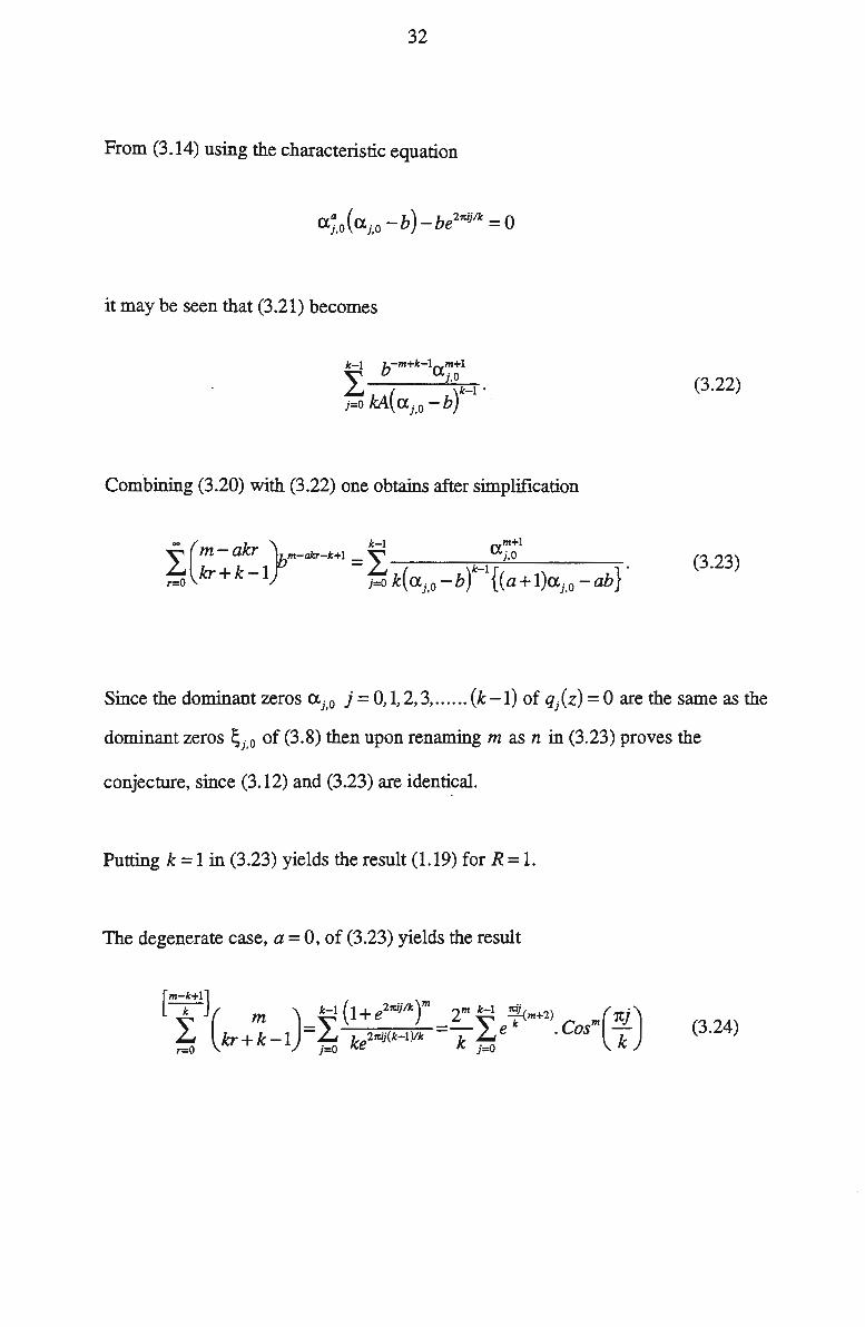
From (3.14) using the characteristic equation

a~ (a . - b)-be2roj/k = O J,0 J,0

it may be seen that (3.21) becomes

k-1 b-m+k-lam+l ~ j ,O

£... ( )k-1 . j=O kA Cl.j,O -b

(3.22)

Combining (3.20) with (3.22) one obtains after simplification

oo ( k J k-1 ,-vm+l ~ m- a r m-akr-k+1 = ~ u.j,O

£... kr + k - l £... k-1 • r=O j=O k( Clj ,O -b) {(a+ l)et.j,O - ab}

(3.23)

Since the dominant zeros aj.o j = 0, 1, 2, 3, ...... (k-1) of q/z) = 0 are the same as the

dominant zeros ~j. o of (3.8) then upon renaming m as n in (3.23) proves the

conjecture, since (3.12) and (3.23) are identical.

Putting k = 1 in (3.23) yields the result (1.19) for R = 1.

The degenerate case, a= 0, of (3.23) yields the result

[m-k+1]

-k- ( m )- k-1 (1 + e2tr.ijlkt - 2m k-1 !f<m+2) m(rcj) L kr + k - l - L 2mj(k-1)1k - Le · Cos r=O j=O ke k j=O k

(3.24)

33

Using the WZ pairs method of Wilf and Zeilberger [ 11] a rational function proof

certificate Rk(m,r) fork= 1and2 of (3.24) is respectively

R1 ( m, r) = ( r ) 2 r-1-m

and ( ) (r-1)(2r-1)

Ri m,r = m(2r-m-2)°

By definition

Gk ( m, r) = ~ ( m, r) ~ ( m, r)

where

( ) ( m )1k-l-m ~ m, r = kr + k -1

and therefore the identity

[m-:-1] L~(m,r)=l r=O

is certified by the pair (~,Gk) with the conditions

~(m+ 1,r )- ~(m,r) =Gk(m,r+ 1)-Gk(m,r)

and limit Gk ( m, r) = 0 satisfied. r"'±oo

34

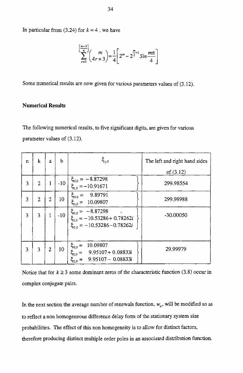
In particular from (3.24) fork= 4, we have

[m-3] ~ ( m )=.!.[2m-2"i+1

Sinm1t] ~ 4r+3 4 4

Some numerical results are now given for various parameters values of (3.12).

Numerical Results

The following numerical results, to five significant digits, are given for various

parameter values of (3.12).

n k a b ~j,O The left and right hand sides

of (3.12)

3 2 1 -10 s 0 0 = - 8.87298 } 299.98554 s10 = -10.91611

~00 = 9.89791 } 3 2 2 10 s1.o = 10.09807 299.98988

3 3 1 -10 ' ~00 = -8.87298 • } -30.00050 s1.0 = -10.53286+ o. 78262i s2.o = -10.53286-0.78262i

~00 = 10.09807

} 3 3 2 10 ~1,0 = 9.95107+ 0.08833i

29.99979

~2,0 = 9.95107- 0.08833i

Notice that fork~ 3 some dominant zeros of the characteristic function (3.8) occur in

complex conjugate pairs.

In the next section the average number of renewals function, wn, will be modified so as

to reflect a non homogeneous difference delay form of the stationary system size

probabilities. The effect of this non homogeneity is to allow for distinct factors,

therefore producing distinct multiple order poles in an associated distribution function.

35

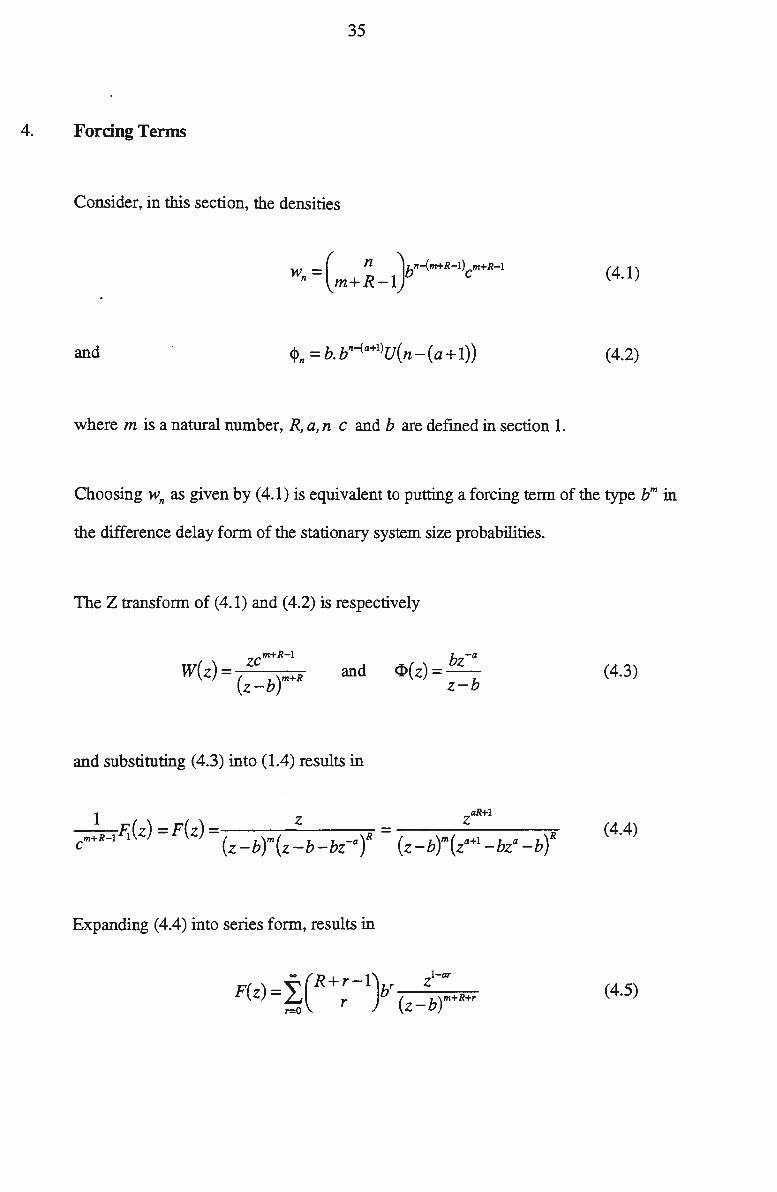
4. Forcing Terms

Consider, in this section, the densities

= ( n )bn-f_m+R-1) m+R-1 w,, m+R-1 c (4.1)

and (4.2)

where m is a natural number, R, a, n c and b are defined in section 1.

Choosing w,, as given by ( 4.1) is equivalent to putting a forcing term of the type bm in

the difference delay form of the stationary system size probabilities.

The Z transform of (4.1) and (4.2) is respectively

ZCm+R-1 W(z) = ( r+R

z-b and <l>(z) = bz-a

z-b (4.3)

and substituting (4.3) into (1.4) results in

1 z zaR+l m+R-1.Fi(z) =F(z) ( r -( ) ( r c ( z - b r z -b -bz-a z - b m za+l - bza -b

(4.4)

Expanding (4.4) into series form, results in

-(R+ r-1) r z1-ar

F(z) = ~ r b (z-bt+R+r (4.5)

36

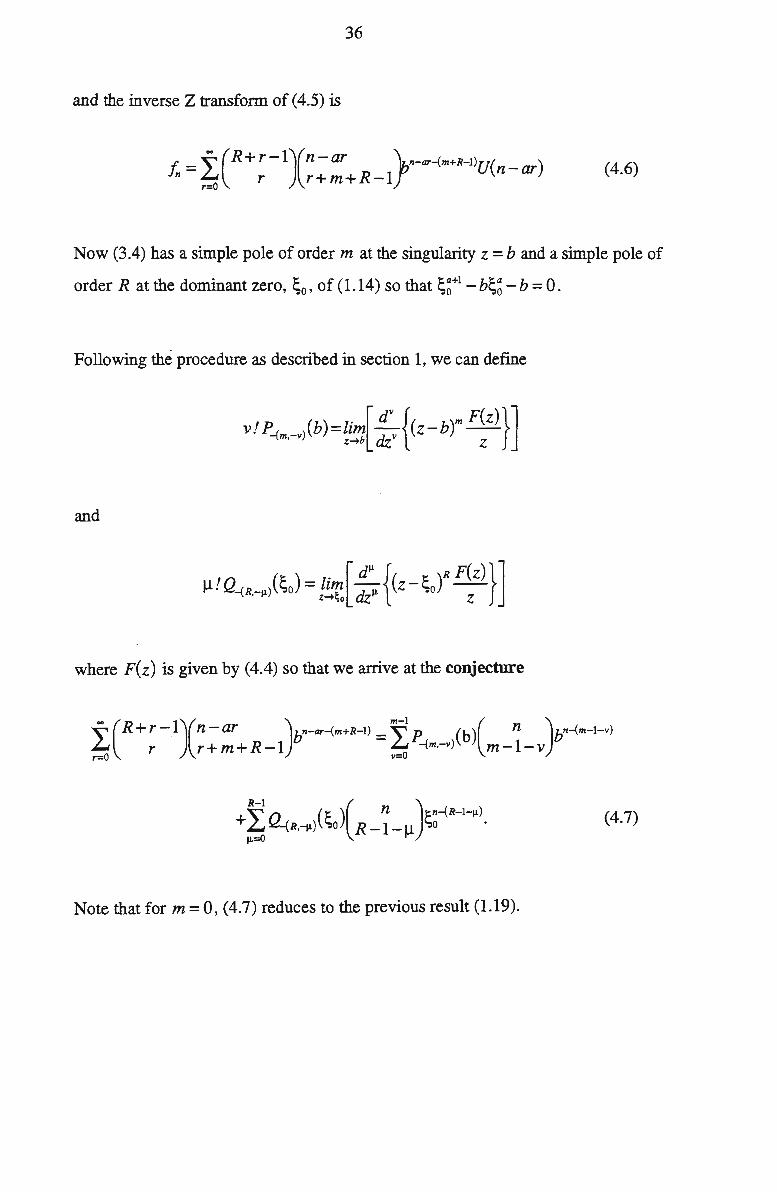
and the inverse Z transform of ( 4.5) is

Now (3.4) has a simple pole of order mat the singularity z =band a simple pole of

order R at the dominant zero, ~0 , of ( 1.14) so that ~~+1 - b~~ - b = 0.

Following the procedure as described in section 1, we can define

v! p_( _ >(b)=lim[!!_{(z-bt F(z)}] m, v Z"°'b dzv Z

and

where F(z) is given by (4.4) so that we arrive at the conjecture

~ (R + r -.l)(n -ar )bn-ar...f_m+R-1) = ~ p (b )( n )bn...f_m-1-v) .£... r r+m+R-1 .£... ...f.m,-v) m-1-v r=O v=O

+ ~ n _ (i: )( n )~11-(R-1-11). ,£...~R.-µ) ~o R-1-µ o µ=O

Note that form= 0, (4.7) reduces to the previous result (1.19).

(4.7)

37

For R = 2andm=1, then from (4.7)

~ (r + l)(n - ar)bn-ar-2 = bn+2a-2 + ~~+l . [(n)A +a( a+ l )( ~ _ b)] (=t r r+2 (~0 -b)A3 1 o

where A= (a+ 1)~0 -ab.

The degenerate case of (4.7), for a== 0 gives the interesting binomial convolution

identity

n-~R+l(R+r-l)( n )= ~(-l)R(R+v-1)( n ) ~ r r+m+R-I ~ v m-1-v r=O v=O

+~(-lt(m+µ-1)( n ) 2n-{R-l-µ) (4_8) ~ µ R-1-µ µ=0

which is in the spirit of the identities given by Chu [4].

For various specific values of m and R the WZ pairs method of Wilf and Zeilberger

may be used to verify the identity (4.8).

38

Appendix A

In section 1, equation (l.31), the identity

abRAQ_(R+l.-•I = ab( R - µ)~,~•.-•I + (A+ ab)~, :r,. ~•.-(•-11)

+(µ- l)AQ-(R-(µ-1)) (Al)

was required.

The identity (Al) can be arrived at in the following way.

From equation ( 1.16)

(A2)

where g(z) is defined by equation (l.14) and ~0 is the dominant zero of g(z).

The equation (A2) can be differentiated with respect to b, such that

where A= (a+ 1)~0 -ab.

39

Simplifying (A3), by adjusting the third term, we obtain

d -R R µ1-n , )=-µin , +-µrn , . db ~R.-µ b . ~R.-µ) b . ~R+l,-µ)

(A4)

Let h(z) = z-ag(z)~0 -A(z- ~0 ) , and obtain a Taylor series expansion of h(z) about

the dominant zero ~0 giving

Substituting (A5) into (A4) we obtain,

d -Rµ! Rµ! µ1-n _ = n , +-Q_ . db ~R.-µ) . b ~R.-µ) b (R+l,-µ)

(A6)

(A7)

Expanding (A6) by the Leibniz differentiation rule gives the result

d -Rµ! Rµ! µ '-Q = n , +-Q_ . db -(R,-µ) b ~R.-µ) b (R+l,-µ)

- R~o 'f(µ)c -k) 'Q r (B )(k) bA ~ k µ . -(R+I,-(µ-k)) z~~ i

(A8)

40

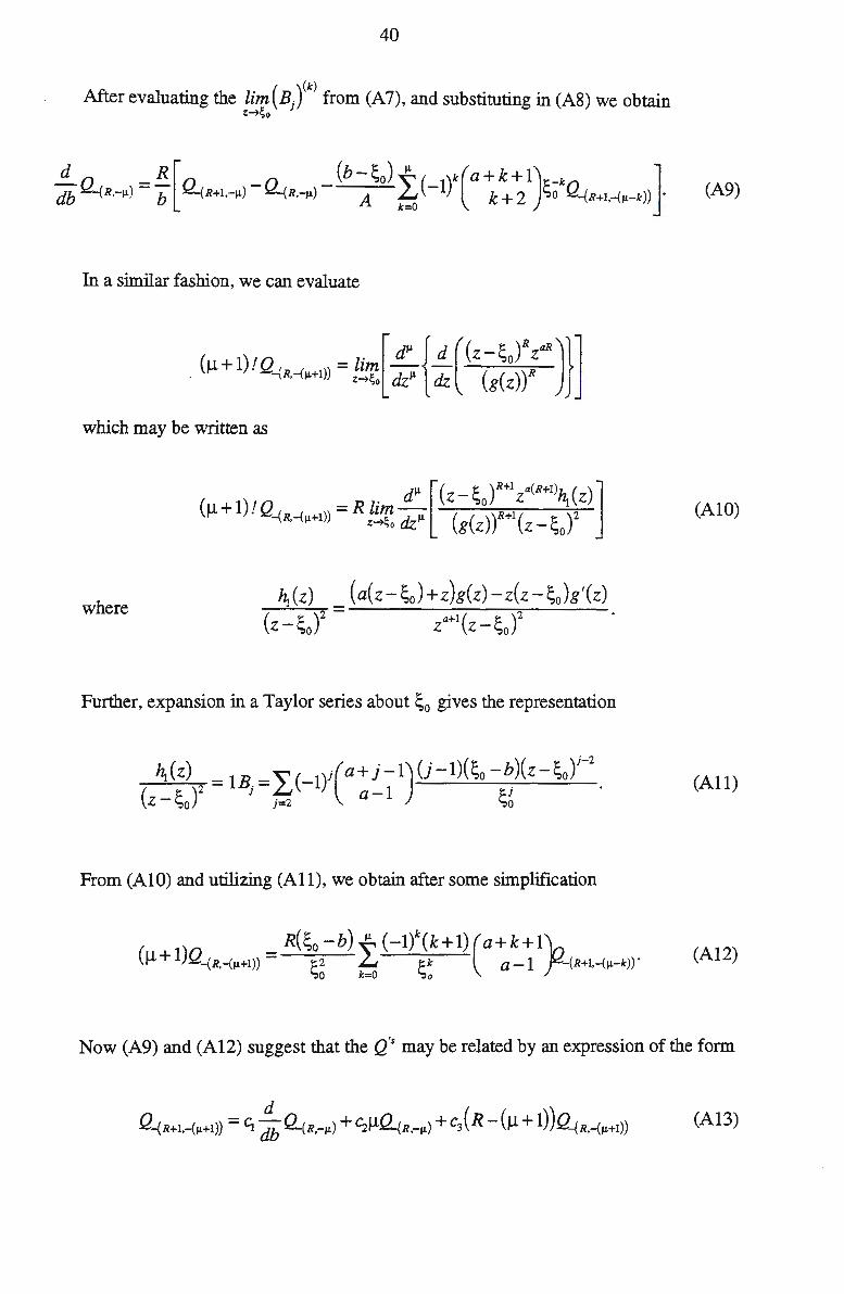
After evaluating the lim(BJ(k) from (A7), and substituting in (A8) we obtain t-t~o

d _ R[ (b-~0)~( )k(a+k+lJ -k ] db ~R.-µ) - b ~R+l,-µ) - ~R.-µ) - A f:'o -1 k + 2 ~o Q-{R+1,-(µ-k)) • (A9)

In a similar fashion, we can evaluate

( 1) / Q _ t [ dµ { d ( ( z - ~o Y zaR )}] · µ + · '-(R.-{µ+i)) - ,~'fo dzµ dz (g(z) Y

which may be written as

1 t - R t z "o z "1 z d µ [( _ ~ )R+l a(R+l)z. ( ) ]

(µ+ ) . Q-(R,-{µ+1)) - ,~'fo dzµ (g(z)y+1(z-~0)2 (AlO)

where ~(z) _ (a(z-~0 )+z)g(z)-z(z-~0 )g'(z)

(z - ~0)2 - za+l(z - ~0)2

Further, expansion in a Taylor series about ~0 gives the representation

~(z) =lB.=I,C-1Y(a+j-1)(j-1)(~0-~)(z-~oY-2 (All) (z-~0)2 ' j=2 a-1 ~~

From (AlO) and utilizing (All), we obtain after some simplification

R(~0 -b) µ (-lt(k+l)(a+k+lp. (µ + l)Q-(R,-{µ+1)) = ~2 L ~k a-1 -(R+I.-{µ-k)) ·

0 k=O o

(A12)

Now (A9) and (A12) suggest that the Q's may be related by an expression of the form

41

for µ = 0, 1, 2, ..... (R-1). The constants £;, c2 and c3 can be evaluated by forming three

simultaneous equations and using the Q values given in table 1 of section I, such that

a+l d µ ~0(R-(µ+l)) Q-{R+I.-(µ+i)) = aR db ~R.-µ) + abR Q_(R.-µ) + AR Q-{R,-(µ+I))

which upon rearrangement and allowing A = (a+ 1 )~0 - ab gives

:b ~•.-•) = Ab (!'+ab) [ abRAQ-{•+1.-{µ+1)) -µAQ-{•.-•l -abl;,( R-(µ + !) )~•.-{µ+1))]. (A14)

. d d Ab Now, smce 7 Q =-Q.-;2

d~0 db -,0

, (A13) can be written as, after rearrangement

~,(A+ ab) ~o ~•.-•) = abRAQ-{R+1,-{µ+1)) - µAQ-{•.-•l - abl;, ( R -(µ + 1} )Q-{R.-(µ+1))

for µ = 0, 1, 2, ...... (R-1)

which is the required identity (Al).

42

AppendixB

Some properties of the zeros of the characteristic functions

g(z) = za+l -bza -b and (Bl)

(B2)

will be discussed in this appendix.

Let b be a real constant , a and k e N , and z is a complex variable, and firstly we

shall consider (Bl).

Theorem 1

(i) The equation (B 1) has at least one and at most two real zeros and a dominant

zero, the one with the greatest modulus, ; 0 such that ; 0 > b for b > 0 and

1; 0 j > _!!:!:._ for b < 0 and the restriction · a+l

(a+1t+1

(abt < l.

(ii) The equation (B2) has at least one and at most four real zeros.

Proof

(B3)

(i) The characteristic equation (B 1) with restriction (B3) has (a+ 1) distinct zeros,

for the derivative of g(z) cannot vanish coincidentally with g(z).

The fact that a related equation to (BI) has distinct zeros appears to have been

reported first by Bailey [2].

..

43

Let G(z) = za(z-b), hence G(z) = b, and the turning point of G(z), away from

th . . ab

e ongm occurs at z = --. a+l

Now consider the graphs of G(z),

For b> 0:

Graph 1:

For b< 0:

a odd

/ a even

f./o /

b -------

The graph of G(z) for a odd or even and b > 0.

a odd

I I

I

Graph 2:

r~

/ ' I \ b J. 1o ,,

--f-~ I

a even

/

b

/ /

I

The graph of G(z) for a odd or even and b < 0.

I

z

44

The two graphs of G(z) indicate therefore that (Bl) has at least one and at

most two real zeros. In both cases of b > 0 and b < 0 it will be shown in the

next theorem that the dominant zero, ~o , the one with the greatest modulus, of

(BI) is always real, such that ~o > b for b > 0 and all a values, and that

l~ol > _:!!!__ for b < 0 and all values of a with restriction (B3). a+I

(ii) In a similar fashion it may be seen that g1 (z) has at most four and at least one

real zeros.

Let G1(z)=(za(z-b)Y , hence Gi(z)=bk and the turningpointof q(z),

f th . . ab

away rom e ongm occurs at z = --. a+I

Now consider the graph of q (z) for b > 0 (the case b < 0 follows in a similar

fashion).

Graph 3:

a even

I I

I a odd

q(z)

-b

The graph of q (z) indicating at least one and at most four real

zeros of g1 (z) with restriction (B3).

45

Theorem2

The characteristic function

q/z) = za+l -bza -be2mjlk

has 'a' zeros on the contour C: lzl :::;; .!!!!__i for each j = 0, 1, 2, 3, .... (k-1) with a+I

restriction (B3).

(B4)

The study of the zeros of (B4), (B2) and (B 1) is important in the area of queueing

theory, and several papers have been devoted to this study, see for example, Chaudhry,

Harris and Marchal [3] and Zhao [16]. Their studies have concentrated, amongst other

things, on robustness of methods for locating zeros inside a unit circle. In this paper

the location of dominant zeros of (Bl), (B2) and (B4) is of prime importance.

Proof

The restriction (B3) comes from (l.20) which is required for the convergence of the

infinite series in equation (l.19).

LetA(z) = -bza. Then A(z) has 'a' zeros in the contour C and

IA(z)I:::;; b(.!!E_)a· a+I

Now

46

( ab )a+l

$ -- +b a+l

By Rouche's theorem, see Takagi [15] , it is required that

hence

(l +(_.!!:_)(_!!!!_)a) < (_!!!!_)a

a+l a+l - a+l

and

l < (_!!!!_)a (-1 ) a+l a+I

which is satisfied since (B3) applies.

Hence the characteristic equation (B4) has 'a' zeros in the contour C and one zero with

modulus bigger than _.!!!!__ . a+l

Now from (B4), letting j = 0 gives the characteristic function (Bl). Theorem 1 now

follows since at least one zero of (B 1) must be real, it is evident that So > b for b > 0

and !sol> _.!!!!__ for b < o. a+l

47

Note, that restriction (B3) is imperative for theorem 2 to apply. If, for example

a = 1, b = .I_, k = 1 which indicates that (B 3) is not satisfied then % ( z) = z2 - ~ - .I. 2 2 2

gives the two zeros as z = {- ~ , 1} , neither of which are in the contour C: lzl ,;; : .

Theorem3

The characteristic function g1 (z) has 'ak' zeros in the contour C:lzl:::;; .!!!?.__ with a+l

restriction (B3).

Proof

Let B(z) =(qj(z)r =(za+1 -bza -be2mj11cy. Utilizing theorem 2, B(z) has therefore

'ak' zeros in the contour C and therefore the remaining 'k' zeros have modulus bigger

than ·l.!!!?._I · a+l

In the contour C,

(BS)

Now,

lg1 (z)- B(z)I =I( G(z))" -bk -(za+I -bza -be2mjtk ti

48

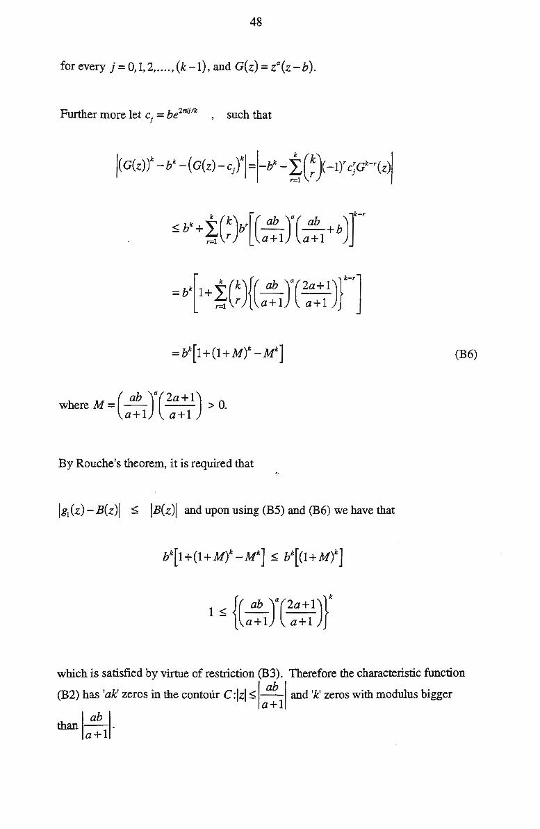
for every j=O,l,2, .... ,(k-1), and G(z)=z0 (z-b).

Further more let cj = be21fijlk , such that

j(G(z))' -b' -(G(z)-c;)'j= -b' -t(~)-1)' c;c'-'(z)

(B6)

h M (ab )

0

(2a+l) O were=-- >. a+l a+l

By Rouche's theorem, it is required that

lg1 (z)-B(z)I ::; IB(z)I and upon using (B5) and (B6) we have that

which is satisfied by virtue of restriction (B3). Therefore the characteristic function

(B2) has 'ak' zeros in the contour C :lzl ::; _.!!:!!_ and 'k' zeros with modulus bigger a+l

than _.!!:!!_ . a+l

49

Consider as, an example a= 3, b = 10, k = 6 such that restriction (B3) is satisfied and

C:lzl ::;;1¥2. The zeros of qj(z) are listed below, showing that one dominant zero

appears from each of the q/z), for j = 0, 12, 3, 4, 5.

qo(z) 10.0100 -0.9696 0.4798- 0.8944i 0.4798+0.8944i

qi (z) 10.0051+0.0086i -0.9157- 0.3231i 0.7697- 0.6786i 0.1412+0.9933i

q2(z) 9.9951+0.0087i -0.7589- 0.6127 i 0.9669- 0.3668 i -0.2031 +0.9708i

%(Z) 9.9900 1.0372 -0.5136+ 0.8375i -0.5136-0.8375i

q4(z) 9.9951-0.0087i -0.7589+0.6127i 0.9669+ 0.3668 i -0.2031-0.9708i

qs(z) 10.0051-0.0086 i -0.9157+0.3231 i 0.7697+0.6786i 0.1412-0.9932i

The dominant zeros of q/z)are listed in the first column and all have modulus bigger

than 7¥2. These dominant zeros are exactly the same k dominant zeros of (B2).

It appears that the zeros, a j (a, b) of equation (B4) can be related for b > 0 and b < 0.

It may be shown that the following relationships hold:

(i) For all values of k and a even

a.j(a,b) =-a./a,-b)

(ii) For k odd and a odd

and,

I

50

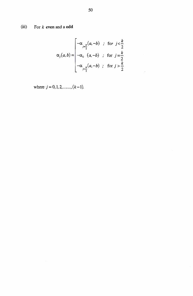
(iii) For k even and a odd

-a "(a,-b) . f . k ' or l<-

"+- 2 J 2

a/a,b) = -CXo (a, -b) . f . k ' or l=-

2

-a . "(a,-b) f . k . or 1 >-' 1- 2 2

where)= 0, 1, 2, ... ... , (k-1).

51

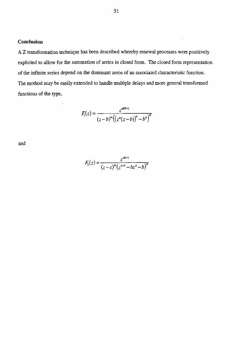
Conclusion

A Z transformation technique has been described whereby renewal processes were positively

exploited to allow for the summation of series in closed form. The closed form representation

of the infinite series depend on the dominant zeros of an associated characteristic function.

The method may be easily extended to handle multiple delays and more general transformed

functions of the type,

and

zaR+1

E(z)--------,~ 2 - { )m( a+l b a b)R z-c z - z -

52

References

[1] ABRAMOWITZ, M. and STEGUN, I. A. Handbook of Mathematical functions.

Dover Publications Inc. New York, 1972.

[2] BAILEY, N. T. J. On Queueing Processes with Bulk Service. Journal of the

Royal Statistical Society B 16, 1954, p 80-87.

[3] CHAUDHRY, M. L., HARRIS, C. M., and MARCHAL, W. G. Robustness of

Rootfinding in single server queueing Models. ORSA Journal of Computing

Vol. 2 (3), 1990 p 273 - 286.

[4] CHU, W. Binomial Convolutions and Hypergeometric Identities. Rendiconti Del

Circolo Matematico Di Palermo. Serie II, Torno XLIII, 1994, p333 - 360.

[5] COHEN, J. W. The Single Server Queue. North-Holland Publishing Company,

Amsterdam, Revised Edition, 1982.

[6] ELA YDI, S. N. An Introduction to Difference Equations. Springer Verlag,

New York, 1996.

[7] GASPER, G. and RAHMAN, M. Basic Hypergeometric Series. Encyclopedia of

Mathematics and its Applications 35. Cambridge University Press, Cambridge, 1990.

[8] GRAHAM, R. L., KNUTH, D. E., and PATASHNIK, 0. Concrete Mathematics.

Addison Wesley, Reading, MA, 1989.

[9] GROSS, D. and HARRIS, C. M. Fundamentals of Queueing Theory. John Wiley and

Sons, New York, 1964.

53

[10] KELLEY, W. G., and PETERSON, A. C. Difference Equation and Introduction with

Applications. Academic Press, Inc., New York, 1991.

[11] PETKOVSEK, M., WILF, H. E., and ZEILBERGER, D. A = B. A. K. Peters,

Wellesley, Massachusetts, 1996.

[12] SAATY, T. L. Elements of Queueing theory with Applications. McGraw Hill Book

Company, New York, 1961.

[13] SLATER, L. J. Generalised Hypergeometricfunctions. Cambridge University Press,

Cambridge, 1966.

[14] SOFO, A. and CERONE, P. On a Fibonacci Related Series. To be published in the

Fibonacci Quarterly.

[15] TAKAGI, H. Queueing Analysis, A Foundation of Peiformance Evaluation, Vol. 1,

Vacation and Priority System, Part 1. North Holland, Amsterdam, 1991.

[16] ZHAO, Y. Analysis of the Gix IM IC, model. Questa 15, 1994, p 347 - 364.

AMS Classification numbers: 05A15, 05A19, 39Al0.