Faculdad de Informatica

Universidad Politecnica de Madrid

Dental Implants SuccessPrediction: Tomography Based

and Data Mining BasedApproach

Master of Science Thesis

Author : Abdallah ELALAILY

Supervisors : Prof. Consuelo Gonzalo

Prof. Ernestina Menasalvas

Submission date : 11 September, 2013

Abstract

There are a number of factors that contribute to the success of dental implantoperations. Among others, is the choice of location in which the prosthetictooth is to be implanted. This project offers a new approach to analyse jawtissue for the purpose of selecting suitable locations for teeth implant oper-ations. The application developed takes as input jaw computed tomographystack of slices and trims data outside the jaw area, which is the point of in-terest. It then reconstructs a three dimensional model of the jaw highlightingpoints of interest on the reconstructed model.On another hand, data mining techniques have been utilised in order to con-struct a prediction model based on an information dataset of previous dentalimplant operations with observed stability values. The goal is to find pat-terns within the dataset that would help predicting the success likelihood ofan implant.

i

Contents

1 Introduction 11.1 Dental implants . . . . . . . . . . . . . . . . . . . . . . . . . . 21.2 Computed tomography . . . . . . . . . . . . . . . . . . . . . . 21.3 Objective . . . . . . . . . . . . . . . . . . . . . . . . . . . . . 21.4 Thesis structure . . . . . . . . . . . . . . . . . . . . . . . . . . 3

2 Background 42.1 Dental implants . . . . . . . . . . . . . . . . . . . . . . . . . . 4

2.1.1 History . . . . . . . . . . . . . . . . . . . . . . . . . . . 42.1.2 Factors affecting osseointegration . . . . . . . . . . . . 5

2.2 Computed tomography scanning . . . . . . . . . . . . . . . . . 52.3 Image processing . . . . . . . . . . . . . . . . . . . . . . . . . 6

2.3.1 Fiji . . . . . . . . . . . . . . . . . . . . . . . . . . . . . 72.4 Data mining . . . . . . . . . . . . . . . . . . . . . . . . . . . . 7

2.4.1 CRISP-DM . . . . . . . . . . . . . . . . . . . . . . . . 82.4.2 Classification analysis . . . . . . . . . . . . . . . . . . . 92.4.3 Weka . . . . . . . . . . . . . . . . . . . . . . . . . . . . 10

3 Approach 113.1 Problem . . . . . . . . . . . . . . . . . . . . . . . . . . . . . . 113.2 Jaw computed tomography slice analysis . . . . . . . . . . . . 11

3.2.1 Visualisation . . . . . . . . . . . . . . . . . . . . . . . 113.2.2 Excess volume cropping . . . . . . . . . . . . . . . . . 123.2.3 Point selection . . . . . . . . . . . . . . . . . . . . . . 17

3.3 Data mining . . . . . . . . . . . . . . . . . . . . . . . . . . . . 21

4 Implementation 234.1 Jaw computed tomography slice analysis . . . . . . . . . . . . 23

4.1.1 Visualisation . . . . . . . . . . . . . . . . . . . . . . . 234.1.2 Excess volume cropping . . . . . . . . . . . . . . . . . 244.1.3 Point selection . . . . . . . . . . . . . . . . . . . . . . 26

ii

4.2 Data mining . . . . . . . . . . . . . . . . . . . . . . . . . . . . 31

5 Results & Discussion 325.1 Tooth marking . . . . . . . . . . . . . . . . . . . . . . . . . . 325.2 Data mining . . . . . . . . . . . . . . . . . . . . . . . . . . . . 36

5.2.1 Naıve Bayes classification . . . . . . . . . . . . . . . . 37

6 Conclusion & Future Work 386.1 Conclusion . . . . . . . . . . . . . . . . . . . . . . . . . . . . . 386.2 Future work . . . . . . . . . . . . . . . . . . . . . . . . . . . . 39

Appendix 40

Bibliography 52

iii

Chapter 1

Introduction

The idea of this study is to find a method that helps predicting the degreeof success of an implant in a certain patient, in a way that would increasethe likelihood success of such operations.

After examining the problem at hand, it was decided that this researchintegrates two approaches. The first one, examining jaw medical imaginingscans to determine what information can be extracted from there. And thesecond involving data mining, in order to look for patterns within records,of already performed operations, to determine if there are in fact patternswithin patient variables that increase or decrease the likelihood of success fordental implant operations.

Over the years, technology improvement within the medical imaging do-main has created more thorough and complex data, that it created the needfor computational systemic ways of extracting information from such images.Biology research thus relies heavily on computer science advances in order toapproach research problems.

The main idea of the research is to automate some analysis techniques toextract information from medical imaging slices in a way that could help in-formation preparation for dental implant operations or other relevant dentalapplications. To do so, we had to get acquainted with the medical aspect ofthe operation, and the rationale behind further studies on the topic. Thiswas conducted in order not to steer away from the practical applications ofthe case we were asked to assist with.

1

Data mining was then thought of as a technique that would create apredictive model for patients undergoing dental implant operations. Datamining would be used to extract on one hand clusters of patients in whichimplants behave similarly, and on the other finding those discriminative fac-tors that may cause the implant operation either success or failure.

1.1 Dental implants

In dentistry, dental implants are root devices used to replace one or moremissing teeth in the human jaw. Dental implants are bolts placed in the hu-man jaw to replace missing teeth. They are normally of metallic structure,usually titanium, made in a way to react with human jaw bone structureso that after healing it becomes difficult to separate from the natural tis-sue. The process by which this occurs is called osseointegration. If a dentalimplant becomes osseointegrated, the implant operation is considered a suc-cessful one. Osseointegration is affected by a number of patient and operationvariables. This is further discussed in the following chapter.

1.2 Computed tomography

X-ray computed tomography is the use of X-rays to acquire tomographic im-ages of specific body parts. The process is used for diagnostic purposes acrossnumerous medical disciplines. Computed tomography produces data thatcould be manipulated in numerous ways to show different physical structuresbased on individual body parts absorption of the X-rays. The tomographicimages are then used to reconstruct a three dimensional representation ofthe scanned volume. Aside from medical applications, computed tomogra-phy also has other applications such as material testing, and archaeologicalscanning.

1.3 Objective

The main goal of this study is to implement computational techniques thatwill further assist dental implant operation planning. Doing so by integrat-ing two approaches. One which dental medical scan files are analysed forinformation that could be deemed beneficial. While the second is to analyse

2

patient related information as well as dental implant parameters to determinefactors that increase or decrease the likelihood of success of dental implantoperations.

1.4 Thesis structure

This thesis consists of 6 chapters, including this one. The following chap-ters are, Background, Approach, Implementation, Results & Discussion andConclusion & Future Work respectively. The Background chapter reviewscontextual information on the technology and software used for the researchproject this document covers. Then, the Approach chapter explains the de-velopment followed for addressing the research problem. Next, the Implemen-tation chapter examines the algorithms developed. After that, the Results& Discussion chapter points out analysis of the results achieved followingthe approach and implementation methodology discussed in the previouschapters. And finally the Conclusion & Future Work chapter covers the im-plications of the research findings and sheds light on the direction of somepossible future work that builds upon the findings of the research.

3

Chapter 2

Background

This chapter discuses the background of concepts and technologies that areused or mentioned throughout this research study.

2.1 Dental implants

2.1.1 History

On a historic level, evidence suggest that dental implants may have datedback to the Ancient Egyptian as early as 3000 B.C.[1][2]. Evidence for den-tal implants were found in Mayan civilisation artifacts that dated back to600 A.D.[2]. Middle-Age Europe, for up until the 17th century, has seenpractices were human teeth were bought off from the poor or corpses to beallotransplanted to other individuals[2]. This practice however involved therisk of spreading infectious diseases.

However, on a medical level, dental implants started taking place aroundthe 1800s, the beginning of the modern surgery era, with concepts of steril-ising and disinfecting surgical apparatus[2]. But in any case, dental implantoperations in a clinical sense was introduced in 1918[3]. The techniques ofthe dental implant operations have changed since then. Modern day den-tal implants rely on a technique discovered by Per-Ingvar Branemark, whileconducting experimentation in which titanium implant chambers were usedto study flow of blood in rabbits’ bones. After however it was time to re-move the chambers from the bone, he realised that bone tissue had com-pletely fussed with the titanium chamber that it has become impossible toremove[4]. Branemark then considered the possibility for human use, and

4

went on to study the effects of titanium implants and bone integration. Heproved that bone tissue could integrate with the titanium oxide layer of animplant that it becomes impossible to separate without fracturing the sur-rounding bone[5]. Branemark named that process osseointegration, derivedfrom the Greek word osteon (bone) and the Latin word integrare (to makewhole).

An implant is said to have osseointegrated when the implant is not ableto show relative movement between its surface and the bone it is in contactwith. In essence the objective is to achieve a stabilising mechanism wherethe prosthetic implant can be incorporated into bone tissue and last undernormal conditions of loading[6].

2.1.2 Factors affecting osseointegration

Several factor may affect osseointegration favourably or unfavourably. Fac-tors that have a favourable effect include implant related factors, such as;implant design, chemical composition, topography of the implant surface,material, shape, diameter, etc. Other factors relate to the implant site, thehost bone tissue and its ability to heal. Furthermore, loading conditions andthe use of adjuvant agents[6].

While factors that might have an unfavourable effect include, excessiveimplant mobility and factors that contribute to that, mismatched coating forthe implant, undergoing radiation therapy, and patient related conditionssuch as; osteoporosis, rheumatoid arthritis, nutritional deficiency, smoking,etc.[6].

2.2 Computed tomography scanning

The use of computed tomography scanning has been cemented in radiologydiagnostics soon following its introduction. The technology was conceived inthe mid 1960s. Sir Godfrey Hounsfield thought of an experimental project inwhich he attempted to reconstruct contents of a box from different readingsat randomly assigned directions. He used a programme to attain absorptionvalues collected, then used another programme to reconstruct those valuesinto a three-dimensional model. Much to his surprise, Sir Hounsfield, foundthe results to be much more accurate than he expected[7].

5

Hounsfield describes the technology as a scanning mechanism in whichX-ray readings are recorded from a number of angles. The data is then trans-lated to absorption values and displayed as a number of pictures (slices). Thetechnology is far more accurate than traditional X-ray systems in a way thatdifferences in tissues of almost the same density can be highlighted. He thenproceeds to describe how the same X-ray technology used in the conventionalway, then, losses precision. Through transforming all information acquiredfrom a three-dimensional body onto a two-dimensional film, where the imageoverlaps objects from back to front. And for which an object to be noticeable,it has to be very different from all the objects that are positioned forwardand backward relative to it[8].

Shortly after the introduction of computed tomography scanning technol-ogy, scan data were taken on tape for processing on an ICL 1905 computer,that required around 20 minutes per slice. Often the reconstruction wouldbe left as an overnight process. The process was thought of as so compli-cated that it would require mainframe processing abilities. However this allchanged as computer technology improved and reconstruction algorithms be-came more efficient[7].

2.3 Image processing

Digital image processing is the process of using computer algorithms to en-hance/show details on raw digital images. The output of image processing iseither an image or image characteristics set that is associated with the inputimage. Image processing maybe be performed for number of reasons:

Image restoration Improving the quality of an image.

Object recognition Detecting different objects in an image.

Pattern recognition Detecting patterns in an image.

Image retrieval Seeking image(s) of interest.

Visualisation Displaying objects that are not clearly visible in an image.

The applications of image processing are numerous, and can range fromtextile manufacturing monitoring to military surveillance operations. Butwhat the diverse applications have in common is the need for storing, pre-processing and then interpreting the raw images.

6

2.3.1 Fiji

Fiji[9] is an open-source image-processing software project that is based onthe skeleton of ImageJ[10]. Fiji addresses problems that underlie with Im-ageJ. For ImageJ is a tool that was developed for biological research by biol-ogists. The result is a software architecture that does not adhere to modernsoftware conventions. Fiji, however, readdresses the outdated architecture,while simultaneously introducing software libraries that deploy a number im-age analysis algorithms.

Fiji is still compatible with ImageJ, while adding extended functionality.In essence, Fiji serves as a distribution of ImageJ that includes additionallibraries and plugins specifically targeting biological image analysis[9].

2.4 Data mining

Knowledge Discovery from Databases (KDD) is defined as the non-trivialtechnique for processing and understanding raw data, and in doing so trans-forming it into data that can be used to give actionable knowledge. The termKDD was put forward in 1989, and it has become prominent in the fields ofartificial intelligence and machine learning since then. To find patterns indata, it incorporates various fields of knowledge such as, statistics, databaseknowledge, machine learning and visualisation. The process includes datacleaning, data storing, machine learning algorithms, processing and visuali-sation.

There are two types of problems, descriptive problems and predictiveproblems. Descriptive problems are problems which data within a dataset isto be interrupted and illustrated in the form of patterns, without the need ofany forecasting. While predictive problems are problems which models aredesigned for information in a dataset in order to anticipate attributes. Theaim of which is to predict an attribute (target variable) based on analysedpatterns in other attributes. For the purpose of this study a predictive modelis needed, and as such classification techniques are utilised to achieve thattarget.

7

2.4.1 CRISP-DM

Data mining process is a far more complex process than applying machinelearning algorithms on a dataset. It is a gradual process that requires infor-mation acquisition and knowledge understanding beforehand. As that is thecase, for the data analytics in this study, the CRISP-DM methodology (CrossIndustry Standard Process for Data Mining) was followed. CRISP-DM is themost used process for data mining projects, and often referred to as the “defacto standard”. CRISP-DM draws guidelines to the phases of developmentthat is to be followed for a data mining project. It also sheds light on thedetails and deliverables of each phase[11].

ProblemUnderstanding

DataUnderstanding

DataPreparation

Modelling

Evaulation

Deployment

Data

Figure 2.1: The phases of CRISP-DM standard model process.

There are 6 phases in the CRISP-DM methodology:

Problem UnderstandingThe initial phase which focusses on understanding the project, itsobjectives and from the business point of view. This includes thor-ough comprehension of different business related aspects, and how theywould relate to one another. The knowledge attained in this phase re-sults in drafting the data mining problem and having a preliminaryplan in order to achieve targeted goals.

Data UnderstandingThis phase aims at comprehending dataset attributes and how they

8

relate to the problem. It starts with initial data collection. This isfollowed by further inspection of the dataset to better one’s under-standing, discovering connections and forming an early hypothesis.

Data PreparationA phase that involves cleaning the initial raw data in order to get toa formal dataset to work on for the later phases. Data preparation islikely to be performed multiple times, as in some cases the data format-ting or selection is constricted by the choice of modelling algorithms.

ModellingIn this phase various machine learning and data mining algorithms areapplied to the dataset. Some algorithms may have specific requirementsregarding the data form. As such, the data preparation phase may berevised.

EvaluationBefore proceeding to the final model deployment, the model is assessedthoroughly and is checked to be in compliance with the predeterminedobjectives. And in doing so reviewing the steps executed to constructthe model.

DeploymentFinally, after passing the evaluation phase, the model is deployed andresults are collected. The creation of the model is generally not the endof the project. Even if the purpose was to increase knowledge of thedata, information will be organised and presented in a way that theend user can use.

2.4.2 Classification analysis

Classification analysis deals with defining a set of categories on data withina dataset whose attributes are known, in other words. The attributes areanalysed and quantised to allow basis for the classification. The purpose oflearning algorithms is to create a classifier given a labelled training set.

Classification analysis not a very exploratory technique. It serves moreof assigning instances to predefined classes, as the objective is to figure outa way of how new instances are to be classified. It is considered as a formof supervised learning, in which a dataset of correctly identified instances isgiven. Some clustering algorithms only work on discrete attributes, and assuch would require preprocessing on numeric based attributes to make them

9

discrete.

Classification analysis is one of pattern recognition algorithms, that serveto assign a kind of output label to given input values. It is a typical approachin data analysis applicable in numerous fields, such as, machine learning, pat-tern recognition, image analysis, information retrieval, and bioinformatics.

2.4.3 Weka

Weka is a machine learning software environment developed at the Univer-sity of Waikato, New Zealand in Java. Weka was developed as it was ob-served that most research in the field of machine learning was focused on therenovation of new machine learning algorithms, whilst little attention wasgiven to expanding existing algorithms to real problem applications. Thedevelopment was focusing on allowing the use of multiple machine learningtechniques that has a simple to use interface with visualisation tools, whilealso allowing some pre- and post-processing tools, with the goal of reachingsupport for scientists in various fields, and not just machine learning ex-perts[12][13].

10

Chapter 3

Approach

This chapter discusses the process that led to the development and imple-mentation of the application as it currently stands.

3.1 Problem

Formally characterised, this study focuses on integrating two approaches withthe main goal of finding a methodology that helps predicting the success ofdental implant operations. The first of which the image analysis of the med-ical image files of the jaw area. The idea being, taking as input a DICOM(Digital Imaging and Communications in Medicine) file stack, and perform-ing investigation based on tissue density differences computed from thosefiles. So as to find information that can be integrated together with thestructured information obtained from patients. This information will be laterused by a knowledge extraction process. Consequently the second approachis to apply data mining techniques to find patterns from the integrated infor-mation. This is done with the objective being creating a model that wouldbe able to calculate the success likelihood of a future dental implant opera-tion based on the variable parameters and how they would fit in the patternsdetected from the dataset analysis.

3.2 Jaw computed tomography slice analysis

3.2.1 Visualisation

The first aspect of the problem is the input, how to handle the informationfiles. Input files in this case are multiple DICOM files per application run.

11

Computed tomography produced volumes of data are windowed around thejaw area. Each file contains a two dimensional horizontal scan of the skull,known as a slice. Slices are then stacked on top of one another bring up threedimensional volumetric data. From there it is possible to render a three di-mensional volume of the scanned body part.

Fiji plug-ins are deployed for the purpose of three dimensional renderingand visualisation of medical scans in this project.

3.2.2 Excess volume cropping

The next aspect is extracting a region of interest from the windowed scanfiles as the entire scan volume contains information that is not needed. Theregions of interest in this case are the locations of individual teeth in thejaw. Any additional tissue that is not trimmed from the scan volume is anunnecessary inefficiency. As it increases the computations throughout therun of the application. And thus it is in the best interest to minimise, asmuch as possible, the unimportant tissue from the application’s perspective.

To deal with this, we thought of doing analysis based on the digital valueof DICOM files. The digital values correspond to the density of the scannedtissues. The idea being, teeth are the most dense tissue in the entire humanbody. As this is the case, scanning an image or a stack volume for the averagemost dense tissue would segment the jaw area (containing teeth) from therest of the scan.

The implementation idea was first tested for two dimensional images, tosee if it holds. Given a two dimensional slice, a box of fixed size traversesthroughout the image, in doing so, calculating the average density at thisspecific location. The location where highest average density is located isstored till all average densities are calculated. After that the region with thehighest average density is highlighted.

As figure 3.1 shows, small-sized average boxes do manage to successfullyhighlight the jaw area, which is our region of interest. However as boxes’sizes increase, the highlighted region switches from the jaw area, to a bitback in the slice. This can be observed clearly in the swtich from an averagebox size of 250× 100 (c) to 300× 125 (d). This takes place because a biggerbox engulfs a lager null area, as the jaw has a relative smaller width than therest of the head on the slice. Despite the relative high density of teeth, thisphenomena disallows a big average box to highlight our region of interest,

12

(a) (b)

(c) (d)

(e) (f)

Figure 3.1: Given a 512×512 slice, the highest average density is highlightedusing average boxes of different sizes; (a) 150×50, (b) 200×75, (c) 250×100,(d) 300 × 125, (e) 350 × 150 and (f) 400 × 175

and instead, highlighting an area that has a more or less monotonic lowerdensity but that does not have null values indicated by the absence of tissue.

This seemed problematic at first, as the technique did not yield the ex-pected result. However, another approach came to mind.

Instead of aiming directly for highlighting the region of interest, the di-rection was changed to use the average calculating box to determine thepoint after which lies the unwanted region. The aspect ratio of the box waschanged, increasing the width to height ratio. And thus, the box would lo-cate the widest region of the scan that has a more or less monotonous densityvalues, and would not select the jaw region as a thin wide box would engulf a

13

(a) (b)

Figure 3.2: Alternative approach using a box with bigger width-to-heightratio in order to mark the monotonous area, which is located directly belowthe region of interest. Again given a 512×512 slice and box sizes (a) 450×75and (b) 500 × 75.

lot of null values at the narrowest region of the scan which corresponds to thejaw. Figure 3.2 shows the results achieved by using the previously describedbox in order to differentiate between rejoins in a jaw slice scan based on theaverage calculated density.

From there, eliminating the unwanted area becomes a trivial problem offiguring out the orientation of the slice, leaving the jaw area in place whileremoving the rest of the tissue below, as shown in figure 3.3.

Figure 3.3: Previous technique deployed to eliminate unwanted region of aslice.

The following step would be to extend this technique to the three di-mensional stack, as opposed to the two dimensional primary implementationpreviously discussed.

14

There were a number of considerations to extend this technique into onemore dimension. The first of which how many degrees of freedom shouldthe average calculating cube be allowed to have. The two dimensional boxhad fixed dimensions based on the best results achieved through the testingprocess. How would adding a new dimension to this affect the outcome wasstill unknown.

It was decided the cube would span the entire stack, and as such be onlyallowed one degree of freedom. The cube has the width of an entire slice,the height of the entire stack and only moves along the y-axis evaluating theaverage density. The results achieved were fairly predictable. The three di-mensional extension of the two dimensional implementation achieved similarresults to those achieved running the two dimensional implementation. Thesame points for extraction were reached in both cases.

But while this removes nearly half of the stack volume, depending onscanning variables as well as the windowing used, this wasn’t enough. Therestill remains unnecessary tissue in the stack. There needs to be further crop-ping to remove the part of the stack which includes the nose in some cases,or the area above the jaw generally speaking. However this was not a simpletask, as some of the scans are upper jaw scans while others are lower jawscans. Deciding which part to remove next would have to rely on figuringout which type of scan the application is dealing with and acting accordingly.

Upper jaw scans are windowed along with the nose tip, while lower jawscans are windowed along with the chin. Examining test data indicated thatthe region of interest is always contained in one half of the remaining scan.

If the scan is of the upper jaw, then the region of interest is in the lowerhalf of the scan, as the upper half contains the nose and middle skull tissue.And if however the scan is of the lower jaw, then thee region of interest isin the upper half of the remaining volume, as the lower jaw is windowedwith the chin and lower skull tissue. The problem then became coming upwith a technique that would figure out which remaining half of the volumeto remove.

A simplistic approach was developed for that sub-problem. Finding thenumber of high value voxels in the remaining scan, the half-volume thatcontains higher number of dense voxels is the half-volume that contains theregion of interest. This stems from the fact that teeth are the highest densitytissue in the human body. And as such, given that the region of interest (jaw)

15

contains at least one tooth, the points with higher density are located there,and the other half of the scan is eliminated. Figure 3.4 shows the results ofthis approach.

(a)

(b)

(c)

Figure 3.4: Two views of the three dimensional reconstruction of the entirestack, (a) before cropping, (b) after removing the back end of the skull (av-erage density cube), and (c) after eliminating further half of the remainingvolume (point of highest intensity).

16

3.2.3 Point selection

After the original scan has been trimmed of unneeded data, there comes thepoint where individual teeth needs to be marked to allow further computa-tions. And while it seems like a trivial task of allocating clusters of highdensity voxels, the task is presented with challenges.

There are a number of factors to consider while planning an algorithmthat performs such a task. Often scan imperfections distort the given data.As a result, two or more teeth could be connected and this from a compu-tational view point be observed as one body after the merging. As well assome voxels of high intensity have been observed in areas where they do notbelong. Furthermore, the lack of uniformity of the space occupied by teethin three dimensional space, caused by different teeth types, positions andorientations, further complicates the task of tooth marking.

The primary purpose of the tooth selection technique was not solely toallocate positions of teeth. But the intention was also to allocate locationswhere teeth used to reside. The rationale was that the site in with a tooth’sroot is fixed to, is of very dense material too. And that those locations willbe highlighted if an algorithm is searching for highly dense voxels. Howeverrepeated tests on different scan cases have concluded that this is not the case.Only the enamel of teeth gets highlighted when looking for highly dense tis-sue in the medical scan. While searching for fairly dense tissue results resultsin highlighting a lot of redundant tissue, that it makes it impossible to pin-point a base of a tooth.After it was confirmed that the selection of both teeth and bases of teethwas not computationally feasible at the moment, it was decided to settle forhighlighting only location of teeth based on the enamel density highlighting.

Much consideration was given to how individual teeth are to be marked ina most computationally efficient manner. And with that in mind, techniquessearching through three dimensional space seemed like performing a lot ofunnecessary computations that would undoubtedly affect the complexity un-favourably. As the three dimensional volume contains information that isredundant for the tooth selection process. The technique developed for ap-proaching this was projecting a threshold version three dimensional volumeof interest down to a two dimensional map. This would in essence simplifygreatly the calculations required to assess the x - and y-axis borders of thebounding box containing the tooth. And in turn, locating the z -axis bound-aries can be performed trivially.

17

In technical terms, the algorithm would traverse the entire region of inter-est, marking voxels that have a value higher than that of the threshold, andplacing those in a two dimensional map. And that serves as a pre-processingphase in order to allocate teeth positions.

After the projection map is attained, it becomes a much simpler task tomark individual tooth locations. The algorithm developed traverses the twodimensional map looking for hits. A hit in this particular incident is definedas a pixel that corresponds in location to a voxel that has a value higherthan that of the threshold. Once a hit is encountered, it is imperative todetermine if this in fact was part of a tooth, and if so the size of the tooth.And if it was a tooth, the location should be marked so that it would notbe revisited in later iterations of the algorithm. This can be a tricky task asteeth are not usually uniform in shape. Which would make searching for thedimensions of the cube/box that engulfs the tooth give inaccurate results ifa simplistic approach was used.

(b) (c) (d)(a)

Figure 3.5: 3-Step Depth Search algorithm, (a) when the algorithm makes ahit is starts to assess the size of the high dense area it has encountered, (b) itfirst steps along the x -axis to determine the end bounds location, (c) alongthat it inspects the vertical bounds, (d) and finally revisiting to horizontalbounds to make sure the entire area is covered within the bounds.

The technique developed particularly for that search case, which we named3-Step Depth Search. In order to accurately find the dimensions, the algo-rithm which starts from one of the leftmost points, proceeds by expandingits search within three steps. The algorithm first encounters a point of highdensity from the leftmost point, and as such the lower x -axis bound is set. Itthen inspects elements to the right of the initial point to see if they lie within

18

this area of high density. With each step in the x direction, it checks for theupper and lower y limits of the area of high density. And furthermore, itsteps again along the x axis looking for the boundary limit. This results inan accurate definition of the bounds of an irregular object.

While this seems like computationally extensive calculations, it is impor-tant to point out that is not performed often, and those nested loop searchesare likely to end quickly as the area covered by the projection of a tooth ontoa two dimensional plane is relatively small. Each iteration halts as soon asit reaches a region outside of what is defined to be a hit.

The technique however, as accurate as it may be, does not account forscan imperfections, in which two or more teeth may appear to be connected.For all it takes is one line of pixels connecting one tooth with another for theselection border to engulf both teeth as one. This is handled by a size checkjust before the tooth’s location is about to be stored. If the size is substan-tially larger than the size of an average tooth, the area is further inspectedfor possible separations between teeth. After a suitable separation is found,the area is then separated into two teeth. That condition keeps evaluatingtill the size of the high density area is deemed suitable to be of one tooth.

(a) (b)

Figure 3.6: Three dimensional reconstruction of a mandible scan showinghigh density bone formation running through the entire jaw, (a) back view,(b) bottom view.

The methodology discussed above runs for two kinds of scan types, max-illa (upper jaw) and mandible (lower jaw) scans. However, as it turns out,

19

there was a complication when running with mandible scans. Mandible scansshowed a unique bone structure features that are not present for maxillascans. Those in turn are of very high density in a way that hindered thealgorithm useless as the entire jaw structure (with or without presence ofteeth) would be marked as one hit spanning all over tooth locations.

Figure 3.6 illustrates the high density bone structure present in mandiblescans. This bone formation results in the entire jaw being positively markedas high density tissue that the algorithm uses as a way to allocate teeth. Assuch, it fails to further mark individual teeth.

The complication was overcome by using statistical methods in order todetermine the average positions of teeth in the mandible. And while havingthe region of interest as the entire jaw, reducing the three dimensional spacethat gets mapped onto a two dimensional plane for tooth marking in a waythat does not let the high density bone structure get in the way of the algo-rithm running.

The running of the plugin previously discussed results in attaining theinput medical scan slices, reconstructed into a three dimensional volume,cropped of unneeded data and with location markers for the positions of ex-isting teeth. While the original purpose of this research was to use thosetooth markers to obtain patterns or information that could otherwise assistin tooth implant operation, time allocated for this project and a number ofsetbacks have disallowed applying further analyses.

20

3.3 Data mining

The CRISP-DM methodology have been followed. First, the problem under-standing phase involved understanding the surgical process and the factorstherein. Doing so to be able to find the information that can be integratedand analysed to find the patterns. And following that, a data mining problemdefinition was obtained. The problem involved finding a predictive model inwhich an osseointegration measure is to be determined. The main goal be-ing, to find the factor of osseointegration based on the clinical informationtogether with the information obtained from the images.

Then came the data understanding phase, which begins with data col-lection, further inspection of the dataset to better one’s understanding, dis-covering connections and forming an early hypothesis. Initial raw data thatwas utilised in order to produce the dataset used for the data mining processwas donated by the dentist who put forward the research topic. Originally,data included two separate work sets. One that included 15 attributes aboutpatients. And another that included 15 attributes about implant operationsperformed on said patients.

The raw data patient attributes contained instances for 32 patients. Thoseattributes are: patient number, age, sex, consultation frequency, oral hygiene,and boolean attributes for: smoking, bruxism, drugs, diabetes, hypertension,hyperparathyroidism, heart disease and osteoporosis, as well as two stringattributes for other conditions and pharmaceutical drugs patients might beon. While the the implant operation data included attributes for 77 implantoperations done on the 32 patients listed before. The collected attributesare: patient number, maxillar dental notation, mandibular dental notation,implant type, length, diameter, drilling method, graft, graft material, sur-gical technique, closing technique, torque, resonance frequency value beforeosseointegration, osseointegration time, resonance frequency value after os-seointegration.

Dental notations use the World Dental Federation notation system (atwo-digit numbering standard used to point to a specific tooth in the jaw).The resonance frequency value is a measure of dental stability calculatedby a hand-held measuring device allowing clinicians to asses the healing ofdental implants. The reading is defined as implant stability quotient whichranges from 0 to 100, 100 being most stable. Readings have a primary valueindicating implant stability and a secondary value indicating changes due tobone formation.

21

Next comes the data preparation phase, which involved cleaning the ini-tial raw data in order to get to a formal dataset to work on for the laterphases. Both sets were merged into one, and attributes were assessed to de-termine their significance for the data mining process. Data cleaning detailsare further discussed int he following chapter.

After that comes the modelling phase, in which modelling techniques areapplied to the dataset. Weka was utilised to apply different classificationtechniques. Weka provides a wide variety of classification algorithms to beapplied to datasets. The dataset was tested with 66 algorithms for the twodental implant stability attributes, resonance frequency value before osseoin-tegration, and resonance frequency value after osseointegration. Resonancefrequency value before osseointegration is the value right after the trans-plant operation is performed. It is not the ultimate measure of success ofan operation, however there is a strong correlation between the resonancefrequency value right after the implant operation and after osseointegration.And as such, a predictive classification model was created for the resonancefrequency value after the implant, and another for the resonance frequencyvalue after osseointegration using the previous resonance frequency value asan attribute of the dataset model.

22

Chapter 4

Implementation

This chapter discusses how the approach process discussed in the previouschapter has been implemented.

The application developed for the purpose of this project is developed asFiji plugin. Fiji is a cross-platform, open-source package based on ImageJ.

4.1 Jaw computed tomography slice analysis

4.1.1 Visualisation

Fiji has a number of plugins that come with the default installation package,as is the case with ImageJ. However, Fiji is more concerned with pluginsthat allows for life sciences research[9].

There was a plugin that comes with the default installation that visualisesstacks in DICOM files, called 3D Viewer. It however was difficult to interpretfor end-users as the visualisation was a single mass blob where tissues exist.There was a necessity of some form of pre-processing. After consideration, itwas decided to go with an edge detecting plugin, which too comes with thedefault installation package. The used plugin is part of the FeatureJ pack-age, and is called FeatureJ Edges. The plugin runs edge detection algorthimsthroughout the volume, and the output is a 3D voulme of the dected edges.The result of the use of those two plugins is a diagram easy to interpret andinteract with.

After the platform for visualising the stack volume was selected, it wastime to assess whether selected platform was suitable for development of the

23

code that does the tasks required for addressing the problem of this research.

4.1.2 Excess volume cropping

As previously discussed, there was a need to separate the region of interest(jaw region) from the rest of scan volume in order to optimise calculationstaking place on the volume through removing unwanted tissue. This takesplace over the course of two steps. The first of which is to find the regionof highest average density, which corresponds to the mid-skull region thatwould engulf the least null values when the calculating average cube movesalong the scan volume. When that region is found, the application proceedsby removing the volume to the back of the cube. The region almost corre-sponds to the back-half of the skull, depending on the scanning variables.

After which, the application then proceeds by further removing half ofthe remaining scan by detecting where the region of interest lies. It looksfor the voxel with the highest intensity, which is placed in the remaining halfof scan that engulfs the region of interest, and removes the other half fromthe scan volume. The result of this step is always a 50% reduction. As thevolume is divided into two based on the number of slices, and one half of thevolume is always removed.

The following is the pseudo-code of the above mentioned functionality.

function segment()

...

get sliceWidth ;

get sliceHeight ;

get NumberofSlices ;

set cubeLength, cubeWidth ;

cubeHeight := NumberofSlices;

HighestAverage := 0;

HighestAveragePosition := 0;

// calculating region with highest average density

for different Y values within image height

for different voxels within cube with dimensions(

cubeLength, cubeWidth, cubeHeight )

get voxelValue;

24

end for

calculate voxelValueAverage;

if voxelValueAverage > HighestAverage

HighestAverage := voxelValueAverage;

HighestAveragePosition := currentY Position;

end if

end for

// removing the back end of the skull

for voxels from HighestAveragePosition till sliceHeight

voxelValue := 0;

end for

// detecting number of voxels with higher intensity

upperHighIntensity := 0, lowerHighIntensity := 0;

for remaining scan voxels

get voxelValue;

if voxelValue > intensityThreshold

if voxel is in upperHalf of scan

upperHighIntensity ++;

else

lowerHighIntensity ++;

end if

end if

end for

if upperHighIntensity > lowerHighIntensity

upper := true;

else

upper := false;

end if

// eliminating the other half of the remaining volume

if upper

for upper half of remaining scan voxels

25

voxelValue := 0;

end for

else

for lower half of remaining scan voxels

voxelValue := 0;

end for

end if

...

end segment

4.1.3 Point selection

As discussed in the approach chapter, the point selection part of the code iswhere most of the plugin functionality is implemented.

The process starts by finding the boundaries of the region of interest,which engulfs all the high dense tissue which at a later point positions ofteeth are to be determined. After that, the three dimensional region of inter-est is projected on a two dimensional boolean plane, where positive values arethose that correspond to the voxels that exceed the value of a tooth intensitythreshold in the three dimensional volume of interest. Once the projectionmap is computed, it is looped upon where positive values trigger a searchingmechanism named 3-Step Depth Search, that determines the size of this re-gion of high dense tissue. If the size is big enough for a tooth, the positionis allocated for the tooth and marked as such so it does not get included infuture iterations of the code. If however the size of the region of interest isbigger than the size of one tooth, it is likely to have been caused by bridgingbetween two or more teeth. The region is inspected for possible separationswithin the region indicating the beginning or end of one tooth. This carrieson until the size of an individual tooth is not computed as too large. Inany case, before any tooth is marked, it is checked that the center positionof the previous tooth is at an adequate distance from the center position ofthe current tooth. As it is the case that sometimes teeth are split into twodue to the size constraint implemented or scan imperfections. If the distancebetween the two centres is too small, the two teeth are merged into one toothengulfing the area that they both are allocated in.

The following is pseudo code that implements the discussed functionality.

26

function teethLocator()

...

get minx, maxx, miny, maxy, minz, maxz ;

//bounding coordinates of the region of interest

boolean[][] projmap := new boolean[maxx -minx ][maxy -miny ];

for voxels within coordinates(minx to maxx, miny to maxy,

minz to maxz )

if voxelValue > threshold

projmap [x][y] := true;

end if

end for

int[][] toothpos := new int[30][4];

toothc := 0;

//array and counter for teeth markers

for points within coordinates(minx to maxx, miny to maxy )

if projmap [x][y] = true

for number of marked teeth

if x and y lie in teethpos

break;

end if

end for

//3-step depth search

offx1 :=1, offyp :=1, offyn :=1, offx2 :=1;

//setting up search offsets

startx :=x, starty :=y, endx :=x, endy :=y;

//setting up tooth boundaries

while x+offx1 <bound && projmap [x+offxp1 ][y]=true

offyp := 1, offyn := 1;

while y+offyp <bound && projmap [x+offxp1 ]

27

[y+offyp ]=true

offx2 := offx1 +1;

while x+offx2 <bound && projmap [x+offx2 ]

[y+offyp ]=true

if endx < x+offx2

endx := x+offx2 ;

end if

offx2 ++;

end while

if endy <y+offyp

starty := y+offyp ;

end if

offyp ++;

end while

while y-offyn >bound && projmap [x+offxp1 ]

[y-offyn ]=true

offx2 := offx1 +1;

while x+offx2 <bound && projmap [x+offx2 ]

[y-offyn ]=true

if endx < x+offx2

endx := x+offx2 ;

end if

offx2 ++;

end while

if starty >y-offyn

starty := y-offyn ;

28

end if

offyn ++;

end while

if endx < x+offx1

endx := x+offx1 ;

end if

end while

//size checking

if toothSize is not too small

while toothSize is too big

if endy -starty > endx -startx

find suitable horizontal separation

add tooth coordinates to toothpos ;

toothc++;

else

find suitable vertical separation

add tooth coordinates to toothpos ;

toothc++;

end if

end while

if toothc > 0

if currentToothCenter-previousToothCenter <

threshold

merge two teeth;

end if

end if

add tooth coordinates to toothpos

toothc++;

end if

29

end if

end for

...

end teethLocator

30

4.2 Data mining

Throughout the data preparation phase, attributes were assessed to deter-mine their significance for the data mining process. It was found that thetext attributes, “other medical conditions” and “pharmaceutical drugs,” willbe of little help to the process. And as they were not of great significance,it was decided not to use those. Also, the attributes “implant type” and“drug use” both had only one value each for all the instances. As such,they will not add anything of value to the model, and they were both dis-carded. As for the “resonance frequency value” attributes, both includedthe primary and secondary numeric values as strings. But as those valueswere of high importance, each text value was split into two numeric values,marking the primary and secondary values of the resonance frequency. Andfinally patient number was discarded after used to merge both data work sets.

The resonance frequency value is the sought variable in the dataset in-stances. The goal of the data mining process is to define how other factorsaffect tooth implant stability. As, however, the dataset does not contain alarge number of instances, it would become especially difficult to attempt topredict the exact numerical figure of the dental stability quotient. It was de-cided to discretise the attributes, each around the mean value of its attribute,distinguishing below average instances from above average instances. Theresonance frequency right after the implant operation is performed, beforeosseointegration, has a mean value of 68.58 and a standard of deviation of8.429, with maximum and minimum values of 86 and 30 respectively. Af-ter allowing time for osseointegration, the mean value becomes 72.74 with a4.601 standard of deviation, 85 as a maximum value and 62 as a minimumvalue. Consequently, for resonance frequency values before osseointegration,values below 68.58 were replaced with below average, while the remainingvalues were replaced with above average. As for values after osseointegra-tion, values above 72.74 were replaced with above average while the restbelow average.

The final size of the dataset after the data cleaning process was 27 at-tributes for each of the 77 instances.

For the modelling phase, Weka was then utilised to use classification algo-rithms which Weka offers to estimate the accuracy of prediction techniques.A total of 66 algorithms compatible with the dataset and the sought at-tributes. The evaluation fo the results achieved is discussed in the followingchapter.

31

Chapter 5

Results & Discussion

This chapter discusses the result achieved from running the developed Fijiplugin with different test case sets. The later part of the chapter discussesthe data mining results.

5.1 Tooth marking

As previously explained the Fiji plugin takes as input medical jaw slices ofeither the maxilla or the mandible and attempts to locate and mark posi-tions that believes to be of tooth positions. The states that will be used toassess the running of the plugin; true positive, in which the plugin correctlyidentifies and marks a tooth position, true negative, correctly not assigninga tooth locator to positions that do not correspond to teeth, false positive,incorrectly placing a tooth locator to a position that does not correspond toa tooth, and false negative, not placing a tooth locator to a position thatcorresponds to a tooth.

Throughout the testing period, it was evident that the scan quality hasa direct correlation to the quality of results achieved. Other variables keptconstant, scans that contained a lot of noise often resulted in poor resultquality, where clean scans often result in better result quality.

Figure 5.1 shows a three dimensional reconstruction of the maxilla scanslices. The figure is shown once clear of the tooth markings, and anotherafter a successful run for the test case. The result shows a success, in whichthere are true positives for all nine teeth positioned in maxilla, along withthe absence of false positives.

32

Figure 5.1: Maxilla test case, all teeth are successfully marked with no falsepositives.

Figure 5.2: Mandible test case, ten of thirteen teeth are successfully marked.The remaining teeth are left unmarked. There are no false positives.

Figure 5.2 shows the plugin run for a mandible test case. The mandiblecontained thirteen teeth, only ten of them were successfully marked. Thismeans there are three cases of false negatives for that particular case. It isalso noticeable that the tooth marker for the second cuspid on the left sideof the mandible is not correctly placed at the center of the tooth. The falsenegatives could be explained by the fact that the incisors and the canineteeth are closely packed. The post processing size segmentation might havenot worked for this case as the size of a number of teeth did not reach thesegmentation threshold size. This is a difficulty that is hard to get around asteeth sizes range from incisors, which are relatively small in size, to molars,which are quite larger. As for the misplaced marker, after viewing the two di-mensional boolean map of the high dense tissue of the volume, it was evidentthat segmentation between the the second cuspid and first molar has been

33

performed at an incorrect place, in a way such that part of the molar toothbecame attached to the molar. This resulted in expanding the x componentof the tooth, and thus centring the marker in the tooth volume of a wrongproportion resulted in a wrong position.

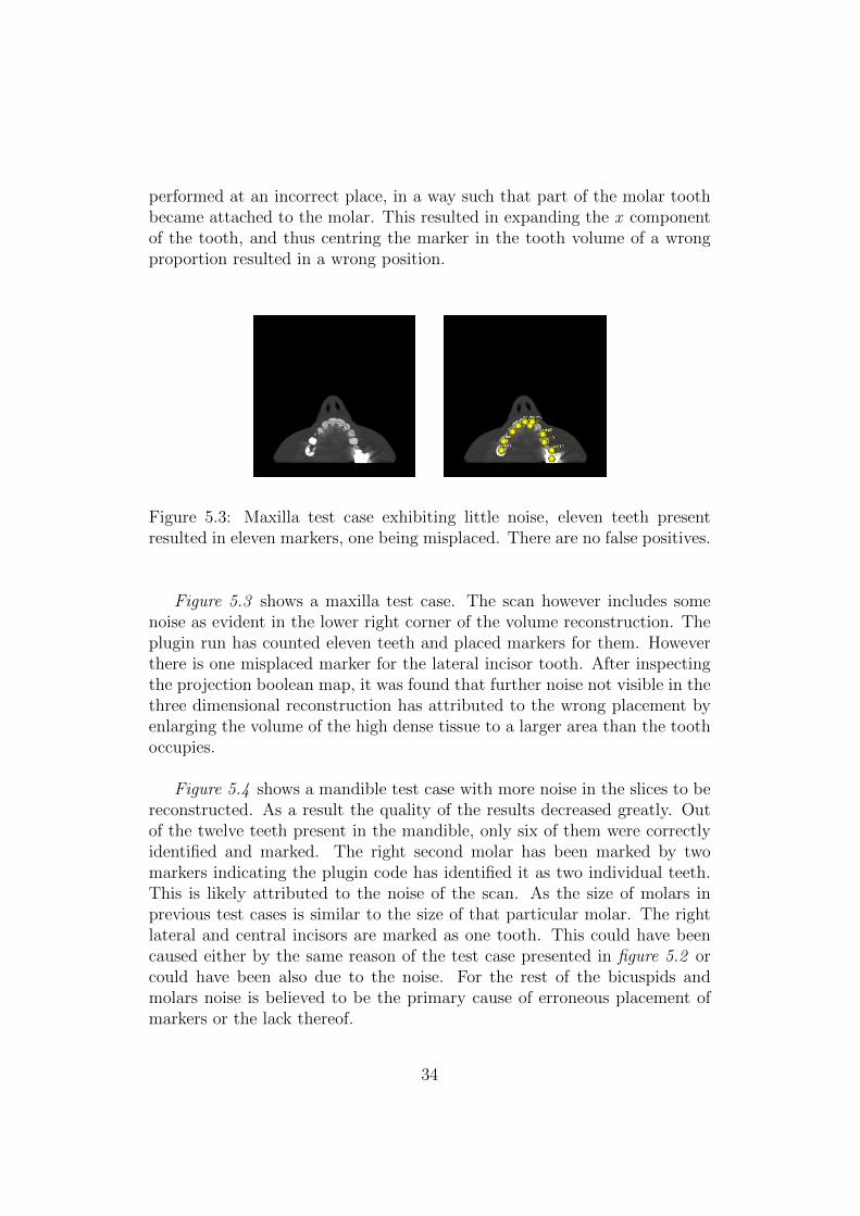
Figure 5.3: Maxilla test case exhibiting little noise, eleven teeth presentresulted in eleven markers, one being misplaced. There are no false positives.

Figure 5.3 shows a maxilla test case. The scan however includes somenoise as evident in the lower right corner of the volume reconstruction. Theplugin run has counted eleven teeth and placed markers for them. Howeverthere is one misplaced marker for the lateral incisor tooth. After inspectingthe projection boolean map, it was found that further noise not visible in thethree dimensional reconstruction has attributed to the wrong placement byenlarging the volume of the high dense tissue to a larger area than the toothoccupies.

Figure 5.4 shows a mandible test case with more noise in the slices to bereconstructed. As a result the quality of the results decreased greatly. Outof the twelve teeth present in the mandible, only six of them were correctlyidentified and marked. The right second molar has been marked by twomarkers indicating the plugin code has identified it as two individual teeth.This is likely attributed to the noise of the scan. As the size of molars inprevious test cases is similar to the size of that particular molar. The rightlateral and central incisors are marked as one tooth. This could have beencaused either by the same reason of the test case presented in figure 5.2 orcould have been also due to the noise. For the rest of the bicuspids andmolars noise is believed to be the primary cause of erroneous placement ofmarkers or the lack thereof.

34

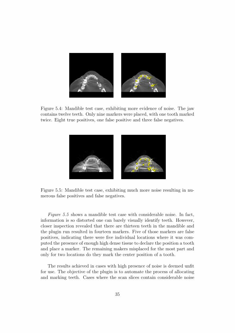
Figure 5.4: Mandible test case, exhibiting more evidence of noise. The jawcontains twelve teeth. Only nine markers were placed, with one tooth markedtwice. Eight true positives, one false positive and three false negatives.

Figure 5.5: Mandible test case, exhibiting much more noise resulting in nu-merous false positives and false negatives.

Figure 5.5 shows a mandible test case with considerable noise. In fact,information is so distorted one can barely visually identify teeth. However,closer inspection revealed that there are thirteen teeth in the mandible andthe plugin run resulted in fourteen markers. Five of those markers are falsepositives, indicating there were five individual locations where it was com-puted the presence of enough high dense tissue to declare the position a toothand place a marker. The remaining makers misplaced for the most part andonly for two locations do they mark the center position of a tooth.

The results achieved in cases with high presence of noise is deemed unfitfor use. The objective of the plugin is to automate the process of allocatingand marking teeth. Cases where the scan slices contain considerable noise

35

hinder the process by causing false calculations that often result in false pos-itives and false negatives.

5.2 Data mining

While testing the data models that predict the stability right after the im-plant operation, before osseointegration, data regarding stability after os-seointegration was eliminated. As the idea is to create a predictive modelthat relies on information available at the time. Testing the stability valueafter osseointegration, included the stability parameter before osseointegra-tion. And thus resulted in an overall better classification success rate due tothe likely strong correlation between the stability values.

For the before osseointegration stability value testing, different algorithmstested on the dataset resulted in classification success that ranged from46.75% to 76.62%. Of the better performing models, Naıve Bayes (71.43%),Lazy Bagging (71.43%), Classification Via Regression (71.43%), LogitBoost(76.62%), Random Committee (75.32%), Rotation Forest (70.13%), VotingFeature Intervals (72.73%), Decision Table/Naıve Bayes Hybrid (71.43%),ADTree (74.03%), Functional Tree (71.43%), NB-Tree (74.02%) and Ran-dom Forest (70.13%).

As for the after osseointegration parameter, different models have a cor-rect classification rate of 62.34% to 84.42%. The models differ with theuse of the stability value before osseointegration as this offer a closer indi-cation to the stability factor after. The successful models in this case are,Bayes Net (83.12%), Naıve Bayes (84.42%), Sequential Minimal Optimisation(80.52%), Attribute Selected Classifier (80.52%), Bagging (83.12%), Dagging(81.82%), Filtered Classifier (80.52%), Random Sub-Space (81.82%), Rota-tion Forest (81.82%), Voting Feature Intervals (81.82%), OneR (83.12%), J48Graft (80.52%), Logistic Model Trees (80.52%), Random Forest (81.82%) andRandom Tree (80.52%).

The inclusiveness of the outcome of classification models could be at-tributed to two factors. The first being there is no strong direct correlationbetween the attributes given in the dataset and the stability parameters.And the second, the number of instances in the dataset is relatively small forclassification techniques to operate adequately.

36

The appendix at the end of this document contains a detailed list of thesummary of results achieved for the different classification and regression al-gorithms tested.

Of the well scoring models tested, it was decided the Naıve Bayes modelprovides a fairly good prediction model for both cases, before as well as afterosseointegration.

5.2.1 Naıve Bayes classification

Naıve Bayes is one of the most powerful inductive learning algorithms formachine learning. Classification is done by applying Bayes rule to computethe portability of the class attribute given a set of attributes. It is a simpleform of Bayesian networking in which all attributes are assumed to be inde-pendent of the class variable, which is called conditional independence. Theconditional independence might not be applicable in real world examples,however the classifier still produce favourable results. This is likely due tothe fact that the classification results most depend on dependencies amongall attributes. It is that dependence between the attributes that affects theclassification[14][15].

37

Chapter 6

Conclusion & Future Work

6.1 Conclusion

The application developed for the purpose of this research performs compu-tations to automatically discover and mark teeth positions in medical scans.It does so by firstly by performing analysis of different scan parts and choos-ing which parts to discard and which to attain for further processing. Afterthat, more fine grain processing is performed, in which structures of highdensity are examined and checked with size constraints. Once the structureis determined is big enough to be that of a tooth, one further size constraintis checked in order to establish that the detected tooth is too big and wasthe likely result of scan imperfections merging two or more teeth together.If that was the case, computations are performed to figure out likely toothboundaries within the high density mass. After all those checks have beenperformed, and the tooth’s position is ready to be marked, one final check isperformed. The last constraint calculates if the current tooth’s center pointis within close proximity with the center point of the tooth before. If the testis positive, it means this is likely caused due to splitting one tooth onto twovolumes. Both teeth are merged back together to be covered by one marker.

The overall accuracy of the markers depends largely on the quality of thescan files. Scan files with considerable noise result in poor quality of results.It is thus imperative to consider the quality in terms of input to obtain qual-ity output.

As for the data mining approach, two probabilistic classifier predictionmodels based on Bayes’ theorem were obtained. The two models attempt toforecast the stability measure of a tooth implant based on other information

38

acquired, one before the operation is performed, and one right after it isperformed and the initial stability value is attained. The model success rateof initial classification ranges from 71.43% to 84.42%.

6.2 Future work

As the time allocated for the project disallowed analysis beyond marking po-sitions of individual teeth within scans of maxillae and mandibles, it thereforeleaves an opportunity for further analysis based on this work and findings.Perhaps even beyond the application for dental implants. It is possible to usethe application developed, or the idea behind the implementation, for a moregeneral approach of other dental problems. And apart from dental problems,the implementation could be adjusted in order to be used for various medicalproblems. Automated way of detecting volumes based on density (high orlow) in various body parts for different applications. And lastly one furtherroom for improvement here might be introduction of additional algorithmconstraints to help increase the precision of the resultant markers.

It remains to be seen if the data mining models could be improved withthe introduction of more information to the dataset. It is likely that in-creasing the dataset instances results in better pattern matching and thusbetter classification. Additional attributes that provide the classification andregression algorithms more information to work on might result in improve-ment in classification success rate of the models.

And finally it would be beneficial if the two implementations were fullyintegrated into one application. Doing so was the motivation of this study.Knowledge discovery and pattern detection working along side tissue densityanalysis, is likely to improve the results achieved for both processes.

39

Appendix.Data mining results usingdifferent classifiers

Resonance frequency value before osseointe-

grationBayes:

Bayes Net:Correctly Classified Instances 52 67.5325%Incorrectly Classified Instances 25 32.4675%Kappa statistic 0.3446Mean absolute error 0.3297Root mean squared error 0.4806Relative absolute error 67.1864%Root relative squared error 96.9831%Total Number of Instances 77

Naıve Bayes:Correctly Classified Instances 55 71.4286%Incorrectly Classified Instances 22 28.5714%Kappa statistic 0.4296Mean absolute error 0.3069Root mean squared error 0.4625Relative absolute error 62.5357%Root relative squared error 93.3351%Total Number of Instances 77

Naıve Bayes Simple:Correctly Classified Instances 55 71.4286%Incorrectly Classified Instances 22 28.5714%Kappa statistic 0.4296Mean absolute error 0.3015Root mean squared error 0.4578Relative absolute error 61.4379%Root relative squared error 92.3787%Total Number of Instances 77

Naıve Bayes Updatable:Correctly Classified Instances 55 71.4286%Incorrectly Classified Instances 22 28.5714%Kappa statistic 0.4296

Mean absolute error 0.3069Root mean squared error 0.4625Relative absolute error 62.5357%Root relative squared error 93.3351%Total Number of Instances 77

Functions:

Logistic:Correctly Classified Instances 50 64.9351%Incorrectly Classified Instances 27 35.0649%Kappa statistic 0.2921Mean absolute error 0.3612Root mean squared error 0.5764Relative absolute error 73.6136%Root relative squared error 116.319%Total Number of Instances 77

Multi-player Perception:Correctly Classified Instances 49 63.6364%Incorrectly Classified Instances 28 36.3636%Kappa statistic 0.2519Mean absolute error 0.3576Root mean squared error 0.5635Relative absolute error 72.871%Root relative squared error 113.716%Total Number of Instances 77

RBF Network:Correctly Classified Instances 53 68.8312%Incorrectly Classified Instances 24 31.1688%Kappa statistic 0.3588Mean absolute error 0.3656Root mean squared error 0.4834Relative absolute error 74.509%

40

Root relative squared error 97.5502%Total Number of Instances 77

Simple Logistic:Correctly Classified Instances 44 57.1429%Incorrectly Classified Instances 33 42.8571%Kappa statistic 0.1283Mean absolute error 0.4237Root mean squared error 0.5027Relative absolute error 86.3485%Root relative squared error 101.449%Total Number of Instances 77

SMO:Correctly Classified Instances 53 68.8312%Incorrectly Classified Instances 24 31.1688%Kappa statistic 0.3731Mean absolute error 0.3117Root mean squared error 0.5583Relative absolute error 63.5179%Root relative squared error 112.662%Total Number of Instances 77

S Pegasos:Correctly Classified Instances 48 62.3377%Incorrectly Classified Instances 29 37.6623%Kappa statistic 0.2509Mean absolute error 0.3766Root mean squared error 0.6137Relative absolute error 76.7508%Root relative squared error 123.842%Total Number of Instances 77

Voted Perceptron:Correctly Classified Instances 50 64.9351%Incorrectly Classified Instances 27 35.0649%Kappa statistic 0.2158Mean absolute error 0.3512Root mean squared error 0.5817Relative absolute error 71.5762%Root relative squared error 117.389%Total Number of Instances 77

Lazy:

IB1:Correctly Classified Instances 48 62.3377%Incorrectly Classified Instances 29 37.6623%Kappa statistic 0.2222Mean absolute error 0.3766Root mean squared error 0.6137Relative absolute error 76.7508%Root relative squared error 123.842%Total Number of Instances 77

IBk:Correctly Classified Instances 48 62.3377%Incorrectly Classified Instances 29 37.6623%Kappa statistic 0.2222Mean absolute error 0.3801Root mean squared error 0.6052

Relative absolute error 77.4575%Root relative squared error 122.126%Total Number of Instances 77

K-Star:Correctly Classified Instances 53 68.8312%Incorrectly Classified Instances 24 31.1688%Kappa statistic 0.3488Mean absolute error 0.346Root mean squared error 0.552Relative absolute error 70.502%Root relative squared error 111.385%Total Number of Instances 77

LWL:Correctly Classified Instances 53 68.8312%Incorrectly Classified Instances 24 31.1688%Kappa statistic 0.3588Mean absolute error 0.3559Root mean squared error 0.4482Relative absolute error 72.5323%Root relative squared error 90.4493%Total Number of Instances 77

Meta:

Ada Boost M1:Correctly Classified Instances 51 66.2338%Incorrectly Classified Instances 26 33.7662%Kappa statistic 0.2946Mean absolute error 0.3561Root mean squared error 0.4668Relative absolute error 72.5626%Root relative squared error 94.1942%Total Number of Instances 77

Attribute Selected Classifier:Correctly Classified Instances 47 61.039%Incorrectly Classified Instances 30 38.961%Kappa statistic 0.186Mean absolute error 0.4138Root mean squared error 0.5187Relative absolute error 84.3354%Root relative squared error 104.665%Total Number of Instances 77

Bagging:Correctly Classified Instances 55 71.4286%Incorrectly Classified Instances 22 28.5714%Kappa statistic 0.4254Mean absolute error 0.3585Root mean squared error 0.4394Relative absolute error 73.059%Root relative squared error 88.6705%Total Number of Instances 77

Classification Via Clustering:Correctly Classified Instances 45 58.4416%Incorrectly Classified Instances 32 41.5584%Kappa statistic 0.1884Mean absolute error 0.4156

41

Root mean squared error 0.6447Relative absolute error 84.6905%Root relative squared error 130.090%Total Number of Instances 77

Classification Via Regression:Correctly Classified Instances 55 71.4286%Incorrectly Classified Instances 22 28.5714%Kappa statistic 0.4167Mean absolute error 0.3812Root mean squared error 0.4657Relative absolute error 77.6936%Root relative squared error 93.9808%Total Number of Instances 77

CV Parameter Selection:Correctly Classified Instances 44 57.1429%Incorrectly Classified Instances 33 42.8571%Kappa statistic 0Mean absolute error 0.4907Root mean squared error 0.4955Relative absolute error 100%Root relative squared error 100%Total Number of Instances 77

Dagging:Correctly Classified Instances 48 62.3377%Incorrectly Classified Instances 29 37.6623%Kappa statistic 0.1976Mean absolute error 0.413Root mean squared error 0.4726Relative absolute error 84.1612%Root relative squared error 95.3753%Total Number of Instances 77

END:Correctly Classified Instances 53 68.8312%Incorrectly Classified Instances 24 31.1688%Kappa statistic 0.3731Mean absolute error 0.3384Root mean squared error 0.4985Relative absolute error 68.9702%Root relative squared error 100.602%Total Number of Instances 77

Filtered Classifier:Correctly Classified Instances 51 66.2338%Incorrectly Classified Instances 26 33.7662%Kappa statistic 0.3106Mean absolute error 0.3888Root mean squared error 0.4979Relative absolute error 79.2243%Root relative squared error 100.475%Total Number of Instances 77

Grading:Correctly Classified Instances 44 57.1429%Incorrectly Classified Instances 33 42.8571%Kappa statistic 0Mean absolute error 0.4286Root mean squared error 0.6547Relative absolute error 87.3371%

Root relative squared error 132.107%Total Number of Instances 77

LogitBoost:Correctly Classified Instances 59 76.6234%Incorrectly Classified Instances 18 23.3766%Kappa statistic 0.5227Mean absolute error 0.304Root mean squared error 0.4228Relative absolute error 61.9565%Root relative squared error 85.3216%Total Number of Instances 77

Multi Boost AB:Correctly Classified Instances 49 63.6364%Incorrectly Classified Instances 28 36.3636%Kappa statistic 0.2462Mean absolute error 0.3522Root mean squared error 0.5386Relative absolute error 71.7689%Root relative squared error 108.683%Total Number of Instances 77

Multi Class Classifier:Correctly Classified Instances 50 64.9351%Incorrectly Classified Instances 27 35.0649%Kappa statistic 0.2921Mean absolute error 0.3612Root mean squared error 0.5764Relative absolute error 73.6136%Root relative squared error 116.316%Total Number of Instances 77

Multi Scheme:Correctly Classified Instances 44 57.1429%Incorrectly Classified Instances 33 42.8571%Kappa statistic 0Mean absolute error 0.4907Root mean squared error 0.4955Relative absolute error 100%Root relative squared error 100%Total Number of Instances 77

Nested Dichotomies, Class Balanced ND:Correctly Classified Instances 53 68.8312%Incorrectly Classified Instances 24 31.1688%Kappa statistic 0.3731Mean absolute error 0.3384Root mean squared error 0.4985Relative absolute error 68.9702%Root relative squared error 100.602%Total Number of Instances 77

Nested Dichotomies, Data Near Balanced ND:Correctly Classified Instances 53 68.8312%Incorrectly Classified Instances 24 31.1688%Kappa statistic 0.3731Mean absolute error 0.3384Root mean squared error 0.4985Relative absolute error 68.9702%Root relative squared error 100.602%Total Number of Instances 77

42

Nested Dichotomies, ND:Correctly Classified Instances 53 68.8312%Incorrectly Classified Instances 24 31.1688%Kappa statistic 0.3731Mean absolute error 0.3384Root mean squared error 0.4985Relative absolute error 68.9702%Root relative squared error 100.602%Total Number of Instances 77

Ordinal Class Classifier:Correctly Classified Instances 53 68.8312%Incorrectly Classified Instances 24 31.1688%Kappa statistic 0.3731Mean absolute error 0.3384Root mean squared error 0.4985Relative absolute error 68.9702%Root relative squared error 100.602%Total Number of Instances 77

Raced Incremental LogitBoost:Correctly Classified Instances 44 57.1429%Incorrectly Classified Instances 33 42.8571%Kappa statistic 0Mean absolute error 0.4907Root mean squared error 0.4955Relative absolute error 100%Root relative squared error 100%Total Number of Instances 77

Random Committee:Correctly Classified Instances 58 75.3247%Incorrectly Classified Instances 19 24.6753%Kappa statistic 0.5019Mean absolute error 0.3095Root mean squared error 0.4456Relative absolute error 63.066%Root relative squared error 89.9243%Total Number of Instances 77

Random Sub Space:Correctly Classified Instances 50 64.9351%Incorrectly Classified Instances 27 35.0649%Kappa statistic 0.2703Mean absolute error 0.3949Root mean squared error 0.4472Relative absolute error 80.4834%Root relative squared error 90.2376%Total Number of Instances 77

Rotation Forest:Correctly Classified Instances 54 70.1299%Incorrectly Classified Instances 23 29.8701%Kappa statistic 0.3878Mean absolute error 0.3438Root mean squared error 0.4511Relative absolute error 70.0655%Root relative squared error 91.041%Total Number of Instances 77

Stacking:

Correctly Classified Instances 44 57.1429%Incorrectly Classified Instances 33 42.8571%Kappa statistic 0Mean absolute error 0.4907Root mean squared error 0.4955Relative absolute error 100%Root relative squared error 100%Total Number of Instances 77

Stacking C:Correctly Classified Instances 44 57.1429%Incorrectly Classified Instances 33 42.8571%Kappa statistic 0Mean absolute error 0.4908Root mean squared error 0.4957Relative absolute error 100.011%Root relative squared error 100.023%Total Number of Instances 77

Threshold Selector:Correctly Classified Instances 36 46.7532%Incorrectly Classified Instances 41 53.2468%Kappa statistic 0.0205Mean absolute error 0.4469Root mean squared error 0.5857Relative absolute error 91.0667%Root relative squared error 118.196%Total Number of Instances 77

Vote:Correctly Classified Instances 44 57.1429%Incorrectly Classified Instances 33 42.8571%Kappa statistic 0Mean absolute error 0.4907Root mean squared error 0.4955Relative absolute error 100%Root relative squared error 100%Total Number of Instances 77

Misc:

Hyper Pipes:Correctly Classified Instances 48 62.3377%Incorrectly Classified Instances 29 37.6623%Kappa statistic 0.1646Mean absolute error 0.4954Root mean squared error 0.4955Relative absolute error 100.951%Root relative squared error 99.9862%Total Number of Instances 77

VFI:Correctly Classified Instances 56 72.7273%Incorrectly Classified Instances 21 27.2727%Kappa statistic 0.4535Mean absolute error 0.381Root mean squared error 0.4751Relative absolute error 77.6338%Root relative squared error 95.8743%Total Number of Instances 77

43

Rules:

Conjunctive Rule:Correctly Classified Instances 48 62.3377%Incorrectly Classified Instances 29 37.6623%Kappa statistic 0.1781Mean absolute error 0.4394Root mean squared error 0.4869Relative absolute error 89.5349%Root relative squared error 98.2536%Total Number of Instances 77

Decision Table:Correctly Classified Instances 47 61.039%Incorrectly Classified Instances 30 38.961%Kappa statistic 0.1667Mean absolute error 0.4482Root mean squared error 0.4996Relative absolute error 91.333%Root relative squared error 100.828%Total Number of Instances 77

DTNB:Correctly Classified Instances 55 71.4286%Incorrectly Classified Instances 22 28.5714%Kappa statistic 0.4254Mean absolute error 0.3326Root mean squared error 0.4299Relative absolute error 67.775%Root relative squared error 86.747%Total Number of Instances 77

JRip:Correctly Classified Instances 50 64.9351%Incorrectly Classified Instances 27 35.0649%Kappa statistic 0.2814Mean absolute error 0.4045Root mean squared error 0.5206Relative absolute error 82.4293%Root relative squared error 105.055%Total Number of Instances 77

NNge:Correctly Classified Instances 53 68.8312%Incorrectly Classified Instances 24 31.1688%Kappa statistic 0.3538Mean absolute error 0.3117Root mean squared error 0.5583Relative absolute error 63.5179%Root relative squared error 112.662%Total Number of Instances 77

OneR:Correctly Classified Instances 43 55.8442%Incorrectly Classified Instances 34 44.1558%Kappa statistic 0.1185Mean absolute error 0.4416Root mean squared error 0.6645Relative absolute error 89.9837%Root relative squared error 134.094%Total Number of Instances 77

PART:Correctly Classified Instances 50 64.9351%Incorrectly Classified Instances 27 35.0649%Kappa statistic 0.2921Mean absolute error 0.3701Root mean squared error 0.5382Relative absolute error 75.4255%Root relative squared error 108.610%Total Number of Instances 77

Ridor:Correctly Classified Instances 49 63.6364%Incorrectly Classified Instances 28 36.3636%Kappa statistic 0.2462Mean absolute error 0.3636Root mean squared error 0.603Relative absolute error 74.1042%Root relative squared error 121.688%Total Number of Instances 77

Zero R:Correctly Classified Instances 44 57.1429%Incorrectly Classified Instances 33 42.8571%Kappa statistic 0Mean absolute error 0.4907Root mean squared error 0.4955Relative absolute error 100%Root relative squared error 100%Total Number of Instances 77

Trees:

AD Tree:Correctly Classified Instances 57 74.026%Incorrectly Classified Instances 20 25.974%Kappa statistic 0.4697Mean absolute error 0.3593Root mean squared error 0.4483Relative absolute error 73.2143%Root relative squared error 90.4604%Total Number of Instances 77

BF Tree:Correctly Classified Instances 53 68.8312%Incorrectly Classified Instances 24 31.1688%Kappa statistic 0.3636Mean absolute error 0.3662Root mean squared error 0.4773Relative absolute error 74.6199%Root relative squared error 96.3261%Total Number of Instances 77

Decision Stump:Correctly Classified Instances 45 58.4416%Incorrectly Classified Instances 32 41.5584%Kappa statistic 0.1515Mean absolute error 0.454Root mean squared error 0.4985Relative absolute error 92.5101%Root relative squared error 100.6039%

44

Total Number of Instances 77

FT:Correctly Classified Instances 55 71.4286%Incorrectly Classified Instances 22 28.5714%Kappa statistic 0.4211Mean absolute error 0.3375Root mean squared error 0.5045Relative absolute error 68.7876%Root relative squared error 101.803%Total Number of Instances 77

J48:Correctly Classified Instances 53 68.8312%Incorrectly Classified Instances 24 31.1688%Kappa statistic 0.3731Mean absolute error 0.3384Root mean squared error 0.4985Relative absolute error 68.9702%Root relative squared error 100.602%Total Number of Instances 77

J48 Graft:Correctly Classified Instances 53 68.8312%Incorrectly Classified Instances 24 31.1688%Kappa statistic 0.3731Mean absolute error 0.3384Root mean squared error 0.4985Relative absolute error 68.9702%Root relative squared error 100.602%Total Number of Instances 77

LAD Tree:Correctly Classified Instances 52 67.5325%Incorrectly Classified Instances 25 32.4675%Kappa statistic 0.3346Mean absolute error 0.3544Root mean squared error 0.5444Relative absolute error 72.2255%Root relative squared error 109.859%Total Number of Instances 77

LMT:Correctly Classified Instances 49 63.6364%Incorrectly Classified Instances 28 36.3636%Kappa statistic 0.2632Mean absolute error 0.3893Root mean squared error 0.4999Relative absolute error 79.3442%Root relative squared error 100.875%Total Number of Instances 77

NB Tree:Correctly Classified Instances 57 74.026%Incorrectly Classified Instances 20 25.974%Kappa statistic 0.4737

Mean absolute error 0.2866Root mean squared error 0.4672Relative absolute error 58.3952%Root relative squared error 94.2863%Total Number of Instances 77

Random Forest:Correctly Classified Instances 54 70.1299%Incorrectly Classified Instances 23 29.8701%Kappa statistic 0.3831Mean absolute error 0.3285Root mean squared error 0.431Relative absolute error 66.941%Root relative squared error 86.9828%Total Number of Instances 77

Random Tree:Correctly Classified Instances 51 66.2338%Incorrectly Classified Instances 26 33.7662%Kappa statistic 0.3106Mean absolute error 0.3485Root mean squared error 0.5745Relative absolute error 71.0161%Root relative squared error 115.936%Total Number of Instances 77

REP Tree:Correctly Classified Instances 53 68.8312%Incorrectly Classified Instances 24 31.1688%Kappa statistic 0.3636Mean absolute error 0.3377Root mean squared error 0.4404Relative absolute error 68.8274%Root relative squared error 88.876%Total Number of Instances 77

Simple Cart:Correctly Classified Instances 53 68.8312%Incorrectly Classified Instances 24 31.1688%Kappa statistic 0.3636Mean absolute error 0.3503Root mean squared error 0.471Relative absolute error 71.3869%Root relative squared error 95.0404%Total Number of Instances 77

User Classifier:Correctly Classified Instances 44 57.1429%Incorrectly Classified Instances 33 42.8571%Kappa statistic 0Mean absolute error 0.4904Root mean squared error 0.4956Relative absolute error 99.9454%Root relative squared error 100.003%Total Number of Instances 77

45

Resonance frequency value after osseointegra-

tionBayers:

Bayes Net:Correctly Classified Instances 64 83.1169%Incorrectly Classified Instances 13 16.8831%Kappa statistic 0.638Mean absolute error 0.1883Root mean squared error 0.3768Relative absolute error 40.0104%Root relative squared error 77.7247%Total Number of Instances 77

Naıve Bayes:Correctly Classified Instances 65 84.4156%Incorrectly Classified Instances 12 15.5844%Kappa statistic 0.6726Mean absolute error 0.172Root mean squared error 0.3636Relative absolute error 36.541%Root relative squared error 74.9882%Total Number of Instances 77

Naıve Bayes Simple:Correctly Classified Instances 65 84.4156%Incorrectly Classified Instances 12 15.5844%Kappa statistic 0.6726Mean absolute error 0.1761Root mean squared error 0.3683Relative absolute error 37.4187%Root relative squared error 75.9631%Total Number of Instances 77

Naıve Bayes Updatable:Correctly Classified Instances 65 84.4156%Incorrectly Classified Instances 12 15.5844%Kappa statistic 0.6726Mean absolute error 0.172Root mean squared error 0.3636Relative absolute error 36.541%Root relative squared error 74.9882%Total Number of Instances 77

Functions:

Logistic:Correctly Classified Instances 54 70.1299%Incorrectly Classified Instances 23 29.8701%Kappa statistic 0.3506Mean absolute error 0.2986Root mean squared error 0.5464Relative absolute error 63.4485%Root relative squared error 112.700%Total Number of Instances 77

Multilayer Perception:Correctly Classified Instances 59 76.6234%

Incorrectly Classified Instances 18 23.3766%Kappa statistic 0.4953Mean absolute error 0.2305Root mean squared error 0.448Relative absolute error 48.9731%Root relative squared error 92.4111%Total Number of Instances 77

RBF Network:Correctly Classified Instances 61 79.2208%Incorrectly Classified Instances 16 20.7792%Kappa statistic 0.5692Mean absolute error 0.23Root mean squared error 0.3935Relative absolute error 48.8627%Root relative squared error 81.1579%Total Number of Instances 77

Simple Logistic:Correctly Classified Instances 60 77.9221%Incorrectly Classified Instances 17 22.0779%Kappa statistic 0.52Mean absolute error 0.2973Root mean squared error 0.3984Relative absolute error 63.1583%Root relative squared error 82.1693%Total Number of Instances 77

SMO:Correctly Classified Instances 62 80.5195%Incorrectly Classified Instances 15 19.4805%Kappa statistic 0.5823Mean absolute error 0.1948Root mean squared error 0.4414Relative absolute error 41.39%Root relative squared error 91.0386%Total Number of Instances 77

S Pegasos:Correctly Classified Instances 55 71.4286%Incorrectly Classified Instances 22 28.5714%Kappa statistic 0.3831Mean absolute error 0.2857Root mean squared error 0.5345Relative absolute error 60.7054%Root relative squared error 110.253%Total Number of Instances 77

Voted Perceptron:Correctly Classified Instances 50 64.9351%Incorrectly Classified Instances 27 35.0649%Kappa statistic 0.0996Mean absolute error 0.3485Root mean squared error 0.5798Relative absolute error 74.0458%Root relative squared error 119.599%Total Number of Instances 77

46

Lazy:

IB1:Correctly Classified Instances 54 70.1299%Incorrectly Classified Instances 23 29.8701%Kappa statistic 0.3595Mean absolute error 0.2987Root mean squared error 0.5465Relative absolute error 63.4647%Root relative squared error 112.731%Total Number of Instances 77

IBk:Correctly Classified Instances 54 70.1299%Incorrectly Classified Instances 23 29.8701%Kappa statistic 0.3595Mean absolute error 0.3044Root mean squared error 0.539Relative absolute error 64.6657%Root relative squared error 111.176%Total Number of Instances 77

K-Star:Correctly Classified Instances 52 67.5325%Incorrectly Classified Instances 25 32.4675%Kappa statistic 0.3132Mean absolute error 0.3251Root mean squared error 0.551Relative absolute error 69.0763%Root relative squared error 113.653%Total Number of Instances 77

LWL:Correctly Classified Instances 59 76.6234%Incorrectly Classified Instances 18 23.3766%Kappa statistic 0.4953Mean absolute error 0.2852Root mean squared error 0.4213Relative absolute error 60.5983%Root relative squared error 86.8995%Total Number of Instances 77

Meta:

Ada Boost M1:Correctly Classified Instances 58 75.3247%Incorrectly Classified Instances 19 24.6753%Kappa statistic 0.4781Mean absolute error 0.2607Root mean squared error 0.4185Relative absolute error 55.3929%Root relative squared error 86.3116%Total Number of Instances 77

Attribute Selected Classifier:Correctly Classified Instances 62 80.5195%Incorrectly Classified Instances 15 19.4805%Kappa statistic 0.5765Mean absolute error 0.2576

Root mean squared error 0.4172Relative absolute error 54.7281%Root relative squared error 86.0595%Total Number of Instances 77

Bagging:Correctly Classified Instances 64 83.1169%Incorrectly Classified Instances 13 16.8831%Kappa statistic 0.6277Mean absolute error 0.2814Root mean squared error 0.3743Relative absolute error 59.7943%Root relative squared error 77.2016%Total Number of Instances 77

Classification via Clustering:Correctly Classified Instances 51 66.2338%Incorrectly Classified Instances 26 33.7662%Kappa statistic 0.3268Mean absolute error 0.3377Root mean squared error 0.5811Relative absolute error 71.7427%Root relative squared error 119.857%Total Number of Instances 77

Classification via Regression:Correctly Classified Instances 60 77.9221%Incorrectly Classified Instances 17 22.0779%Kappa statistic 0.5392Mean absolute error 0.2465Root mean squared error 0.3543Relative absolute error 52.3799%Root relative squared error 73.0873%Total Number of Instances 77

CV Parameter Selection:Correctly Classified Instances 48 62.3377%Incorrectly Classified Instances 29 37.6623%Kappa statistic 0Mean absolute error 0.4707Root mean squared error 0.4848Relative absolute error 100%Root relative squared error 100%Total Number of Instances 77

Dagging:Correctly Classified Instances 63 81.8182%Incorrectly Classified Instances 14 18.1818%Kappa statistic 0.6074Mean absolute error 0.3Root mean squared error 0.3798Relative absolute error 63.7406%Root relative squared error 78.3496%Total Number of Instances 77

END:Correctly Classified Instances 60 77.9221%Incorrectly Classified Instances 17 22.0779%Kappa statistic 0.5132Mean absolute error 0.2614Root mean squared error 0.4241Relative absolute error 55.5291%

47

Root relative squared error 87.4735%Total Number of Instances 77

Filtered Classifier:Correctly Classified Instances 62 80.5195%Incorrectly Classified Instances 15 19.4805%Kappa statistic 0.5765Mean absolute error 0.2573Root mean squared error 0.3985Relative absolute error 54.6747%Root relative squared error 82.2002%Total Number of Instances 77

Grading:Correctly Classified Instances 48 62.3377%Incorrectly Classified Instances 29 37.6623%Kappa statistic 0Mean absolute error 0.3766Root mean squared error 0.6137Relative absolute error 80.0207%Root relative squared error 126.584%Total Number of Instances 77

LogitBoost:Correctly Classified Instances 59 76.6234%Incorrectly Classified Instances 18 23.3766%Kappa statistic 0.5022Mean absolute error 0.2495Root mean squared error 0.3963Relative absolute error 53.0016%Root relative squared error 81.7522%Total Number of Instances 77

Multi-Boost AB:Correctly Classified Instances 61 79.2208%Incorrectly Classified Instances 16 20.7792%Kappa statistic 0.5513Mean absolute error 0.218Root mean squared error 0.4514Relative absolute error 46.3175%Root relative squared error 93.1051%Total Number of Instances 77

Multi-Class Classifier:Correctly Classified Instances 54 70.1299%Incorrectly Classified Instances 23 29.8701%Kappa statistic 0.3506Mean absolute error 0.2986Root mean squared error 0.5464Relative absolute error 63.4485%Root relative squared error 112.700%Total Number of Instances 77

Multi-Scheme:Correctly Classified Instances 48 62.3377%Incorrectly Classified Instances 29 37.6623%Kappa statistic 0Mean absolute error 0.4707Root mean squared error 0.4848Relative absolute error 100%Root relative squared error 100%Total Number of Instances 77

Nested Dichotomies, Class Balanced ND:Correctly Classified Instances 60 77.9221%Incorrectly Classified Instances 17 22.0779%Kappa statistic 0.5132Mean absolute error 0.2614Root mean squared error 0.4241Relative absolute error 55.5291%Root relative squared error 87.4735%Total Number of Instances 77

Nested Dichotomies, Data Near Balanced ND:Correctly Classified Instances 60 77.9221%Incorrectly Classified Instances 17 22.0779%Kappa statistic 0.5132Mean absolute error 0.2614Root mean squared error 0.4241Relative absolute error 55.5291%Root relative squared error 87.4735%Total Number of Instances 77

Nested Dichotomies, ND:Correctly Classified Instances 60 77.9221%Incorrectly Classified Instances 17 22.0779%Kappa statistic 0.5132Mean absolute error 0.2614Root mean squared error 0.4241Relative absolute error 55.5291%Root relative squared error 87.4735%Total Number of Instances 77

Ordinal Class Classifier:Correctly Classified Instances 60 77.9221%Incorrectly Classified Instances 17 22.0779%Kappa statistic 0.5132Mean absolute error 0.2614Root mean squared error 0.4241Relative absolute error 55.5291%Root relative squared error 87.4735%Total Number of Instances 77

Raced Incremental LogitBoost:Correctly Classified Instances 48 62.3377%Incorrectly Classified Instances 29 37.6623%Kappa statistic 0Mean absolute error 0.4707Root mean squared error 0.4848Relative absolute error 100%Root relative squared error 100%Total Number of Instances 77

Random Committee:Correctly Classified Instances 59 76.6234%Incorrectly Classified Instances 18 23.3766%Kappa statistic 0.4953Mean absolute error 0.2549Root mean squared error 0.3873Relative absolute error 54.1562%Root relative squared error 79.8814%Total Number of Instances 77

Random Sub Space:

48

Correctly Classified Instances 63 81.8182%Incorrectly Classified Instances 14 18.1818%Kappa statistic 0.6019Mean absolute error 0.3271Root mean squared error 0.39Relative absolute error 69.4995%Root relative squared error 80.4455%Total Number of Instances 77

Rotation Forest:Correctly Classified Instances 63 81.8182%Incorrectly Classified Instances 14 18.1818%Kappa statistic 0.6074Mean absolute error 0.2462Root mean squared error 0.3545Relative absolute error 52.3201%Root relative squared error 73.1244%Total Number of Instances 77

Stacking:Correctly Classified Instances 48 62.3377%Incorrectly Classified Instances 29 37.6623%Kappa statistic 0Mean absolute error 0.4707Root mean squared error 0.4848Relative absolute error 100%Root relative squared error 100%Total Number of Instances 77

Stacking C:Correctly Classified Instances 48 62.3377%Incorrectly Classified Instances 29 37.6623%Kappa statistic 0Mean absolute error 0.4705Root mean squared error 0.4848Relative absolute error 99.976%Root relative squared error 99.999%Total Number of Instances 77

Threshold Selector:Correctly Classified Instances 52 67.5325%Incorrectly Classified Instances 25 32.4675%Kappa statistic 0.3568Mean absolute error 0.3121Root mean squared error 0.5159Relative absolute error 66.3138%Root relative squared error 106.422%Total Number of Instances 77

Vote:Correctly Classified Instances 48 62.3377%Incorrectly Classified Instances 29 37.6623%Kappa statistic 0Mean absolute error 0.4707Root mean squared error 0.4848Relative absolute error 100%Root relative squared error 100%Total Number of Instances 77

Misc:

Hyper Pipes:Correctly Classified Instances 50 64.9351%Incorrectly Classified Instances 27 35.0649%Kappa statistic 0.3468Mean absolute error 0.4925Root mean squared error 0.4927Relative absolute error 104.633%Root relative squared error 101.617%Total Number of Instances 77

VFI:Correctly Classified Instances 63 81.8182%Incorrectly Classified Instances 14 18.1818%Kappa statistic 0.618Mean absolute error 0.3601Root mean squared error 0.4537Relative absolute error 76.5165%Root relative squared error 93.5814%Total Number of Instances 77

Rules:

Conjunctive Rule:Correctly Classified Instances 59 76.6234%Incorrectly Classified Instances 18 23.3766%Kappa statistic 0.4953Mean absolute error 0.2991Root mean squared error 0.4343Relative absolute error 63.5447%Root relative squared error 89.5814%Total Number of Instances 77

Decision Table:Correctly Classified Instances 59 76.6234%Incorrectly Classified Instances 18 23.3766%Kappa statistic 0.5022Mean absolute error 0.3198Root mean squared error 0.4112Relative absolute error 67.9443%Root relative squared error 84.8189%Total Number of Instances 77

DTNB:Correctly Classified Instances 60 77.9221%Incorrectly Classified Instances 17 22.0779%Kappa statistic 0.52Mean absolute error 0.268Root mean squared error 0.413Relative absolute error 56.9399%Root relative squared error 85.1864%Total Number of Instances 77

J Rip:Correctly Classified Instances 61 79.2208%Incorrectly Classified Instances 16 20.7792%Kappa statistic 0.5575Mean absolute error 0.2714Root mean squared error 0.4147Relative absolute error 57.6578%Root relative squared error 85.5477%Total Number of Instances 77

49

NNge:Correctly Classified Instances 59 76.6234%Incorrectly Classified Instances 18 23.3766%Kappa statistic 0.4882Mean absolute error 0.2338Root mean squared error 0.4835Relative absolute error 49.668%Root relative squared error 99.7278%Total Number of Instances 77

OneR:Correctly Classified Instances 64 83.1169%Incorrectly Classified Instances 13 16.8831%Kappa statistic 0.6429Mean absolute error 0.1688Root mean squared error 0.4109Relative absolute error 35.8714%Root relative squared error 84.7523%Total Number of Instances 77

PART:Correctly Classified Instances 59 76.6234%Incorrectly Classified Instances 18 23.3766%Kappa statistic 0.4953Mean absolute error 0.2639Root mean squared error 0.4523Relative absolute error 56.0758%Root relative squared error 93.3012%Total Number of Instances 77

Ridor:Correctly Classified Instances 58 75.3247%Incorrectly Classified Instances 19 24.6753%Kappa statistic 0.4709Mean absolute error 0.2468Root mean squared error 0.4967Relative absolute error 52.4274%Root relative squared error 102.460%Total Number of Instances 77

Zero R:Correctly Classified Instances 48 62.3377%Incorrectly Classified Instances 29 37.6623%Kappa statistic 0Mean absolute error 0.4707Root mean squared error 0.4848Relative absolute error 100%Root relative squared error 100%Total Number of Instances 77

Trees:

AD Tree:Correctly Classified Instances 60 77.9221%Incorrectly Classified Instances 17 22.0779%Kappa statistic 0.533Mean absolute error 0.2804Root mean squared error 0.4023Relative absolute error 59.585%Root relative squared error 82.9842%

Total Number of Instances 77

BF Tree:Correctly Classified Instances 60 77.9221%Incorrectly Classified Instances 17 22.0779%Kappa statistic 0.5266Mean absolute error 0.2838Root mean squared error 0.4247Relative absolute error 60.3043%Root relative squared error 87.6044%Total Number of Instances 77

Decision Stump:Correctly Classified Instances 61 79.2208%Incorrectly Classified Instances 16 20.7792%Kappa statistic 0.5513Mean absolute error 0.2934Root mean squared error 0.4129Relative absolute error 62.3401%Root relative squared error 85.177%Total Number of Instances 77

FT:Correctly Classified Instances 60 77.9221%Incorrectly Classified Instances 17 22.0779%Kappa statistic 0.5266Mean absolute error 0.235Root mean squared error 0.4496Relative absolute error 49.9202%Root relative squared error 92.7267%Total Number of Instances 77

J48:Correctly Classified Instances 60 77.9221%Incorrectly Classified Instances 17 22.0779%Kappa statistic 0.5132Mean absolute error 0.2614Root mean squared error 0.4241Relative absolute error 55.5291%Root relative squared error 87.4735%Total Number of Instances 77

J48 Graft:Correctly Classified Instances 62 80.5195%Incorrectly Classified Instances 15 19.4805%Kappa statistic 0.5643Mean absolute error 0.2469Root mean squared error 0.411Relative absolute error 52.4631%Root relative squared error 84.7806%Total Number of Instances 77

LAD Tree:Correctly Classified Instances 61 79.2208%Incorrectly Classified Instances 16 20.7792%Kappa statistic 0.5513Mean absolute error 0.2788Root mean squared error 0.4432Relative absolute error 59.2295%Root relative squared error 91.4243%Total Number of Instances 77

50

LMT:Correctly Classified Instances 62 80.5195%Incorrectly Classified Instances 15 19.4805%Kappa statistic 0.5823Mean absolute error 0.2575Root mean squared error 0.3887Relative absolute error 54.7017%Root relative squared error 80.1696%Total Number of Instances 77

NB Tree:Correctly Classified Instances 53 68.8312%Incorrectly Classified Instances 24 31.1688%Kappa statistic 0.3451Mean absolute error 0.312Root mean squared error 0.5062Relative absolute error 66.2947%Root relative squared error 104.4028%Total Number of Instances 77

Random Forest:Correctly Classified Instances 63 81.8182%Incorrectly Classified Instances 14 18.1818%Kappa statistic 0.6074Mean absolute error 0.2528Root mean squared error 0.3621Relative absolute error 53.7151%Root relative squared error 74.6926%Total Number of Instances 77

Random Tree:Correctly Classified Instances 62 80.5195%Incorrectly Classified Instances 15 19.4805%Kappa statistic 0.5765Mean absolute error 0.2011

Root mean squared error 0.4432Relative absolute error 42.7343%Root relative squared error 91.4109%Total Number of Instances 77

Rep Tree:Correctly Classified Instances 58 75.3247%Incorrectly Classified Instances 19 24.6753%Kappa statistic 0.4781Mean absolute error 0.318Root mean squared error 0.4516Relative absolute error 67.5629%Root relative squared error 93.144%Total Number of Instances 77

Simple Cart:Correctly Classified Instances 60 77.9221%Incorrectly Classified Instances 17 22.0779%Kappa statistic 0.52Mean absolute error 0.2993Root mean squared error 0.4339Relative absolute error 63.5823%Root relative squared error 89.5084%Total Number of Instances 77

User Classifier:Correctly Classified Instances 48 62.3377%Incorrectly Classified Instances 29 37.6623%Kappa statistic 0Mean absolute error 0.4698Root mean squared error 0.4848Relative absolute error 99.82%Root relative squared error 99.999%Total Number of Instances 77

51

Bibliography

[1] Irish, J. (2004). A 5,500 year old artificial human tooth from Egypt: ahistorical note. The International Journal of Oral and MaxillofacialSurgery, 19 (5), p: 645-647.

[2] Ring, M. (1995). A Thousand Years of Dental Implants: A DefinitiveHistory-Part 1. Compendium of Continuing Education in Dentistry,16 (10), p: 1060-1690.

[3] Ring, M. (1995). A Thousand Years of Dental Implants: A DefinitiveHistory-Part 2. Compendium of Continuing Education in Dentistry,16 (11), p: 1132-1152.

[4] Branemark, P. (1959). Vital microscopy of bone marrow in rabbit. Scan-dinavian Journal of Clinical and Laboratory Investigation, 11 (38), p:1-82.

[5] Branemark, P. (1983). Osseointegration and its experimental back-ground. The Journal of Prosthetic Dentistry, 50 (3), p: 399-410.doi:10.1016/S0022-3913(83)80101-2

[6] Mavrogenis, A., Dimitriou, R., Parvizi, J. & Babis, G. (2009). Biologyof Implant Osseointegration. Journal of Musculoskeletal and NeuronalInteractions 9 (2), p: 61-71.

[7] Beckmann, E. (2006). CT scanning the early days. The British Journalof Radiology, 79, p: 5-8. doi:10.1259/bjr/29444122

[8] Hounsfield, G. (1973). Computerized Transverse Axial Scanning (to-mography): Part 1. Description of system. The British Journal ofRadiology, 46, p: 1016-1022. doi:10.1259/0007-1285-46-552-1016

[9] Schindelin, J., et al. (2012). Fiji: An Open-Source Platform forBiological-Image Analysis. Nature Methods, 9 (7), p: 676-682. doi:10.1038/nmeth.2019

52

[10] Schneider, C., Rasband, W. & Eliceiri, K. (2012). NIH Image to Im-ageJ: 25 years of image analysis. Nature Methods, 9 (7), p: 671-675.doi:10.1038/nmeth.2089

[11] Marban, O., Mariscal, G. & Segovia, J. (2009). A Data Mining & Knowl-edge Discovery Process Model (p: 438-453). Vienna, Austria: In-Teh.

[12] Holmes, G., Donkin, A. & Witten, I. (1994). WEKA: A Machine Learn-ing Workbench. Proceedings of Second Australia and New ZealandConference on Intelligent Information Systems.

[13] Garner, S., Cunningham, S., Holmes, G., Nevill-Manning, C. & Witten,I. (1995). Applying a Machine Learning Workbench: Experience withAgricultural Databases. Proceedings of Machine Learning in PracticeWorkshop, Machine Learning Conference, p: 14-21.

[14] Zhang, H. (2004). The Optimality of Naive Bayes. Florida ArtificialIntelligence Research Society, proceedings of FLAIRS Conference 2004,p: 562-567.

[15] Othman, M. & Yau T. (2007). Comparison of Different ClassificationTechniques Using WEKA for Breast Cancer. International Conferenceon Biomedical Engineering, proceedings of IFMBE Conference 2007,15, p: 520-523.

53