Density extraction from P-wave AVO inversion: Tuscaloosa Trend example

Jyoti Behura1, Nurul Kabir2, Richard Crider2, Petr J́ılek2, and Ellen Lake3

1Center for Wave Phenomena, Colorado School of Mines, Golden, Colorado 80401, USA; 2BP Explorationand Production Technology Group, Houston, Texas 77079, USA; 3BP North American Gas StrategicPerformance Unit, Houston, Texas 77079, USA.

Summary

Density extraction from AVO inversion is thought to beunstable and difficult. Recent research has, however,shown that it is possible to extract density reliably fromP-wave reflection data if the density contrast is significantacross the interface. This approach is tested over a gasreservoir where petrophysical evidence suggests thatdensity is the primary driver of reflectivity. By adoptinga linear as well as a non-linear approach, inversion isperformed for density and P-wave velocity from a 3Dprestack seismic dataset acquired over this gas reservoir.The non-linear inversion results agree well with the logand production data, thus proving that density can beextracted reliably in this case and used for reservoircharacterization. We use the extracted density alongwith the P-wave velocity to distinguish the low-densityporous gas sands from wet sands, tight sands, andshales.

Introduction

The Tuscaloosa Trend, located in South Louisiana, is aseries of gas fields. All these sands are of Cretaceous ageand were deposited in a near-shore marine depositionalenvironment. Data from a 3D seismic survey over thisarea is used in this study. Lithology at the reservoirdepths consists of gas-saturated sands along with wetsands, tight sands, and shales. Reduction of drilling riskand optimization of production requires delineating andseparating gas sands from other lithologies.

Amplitude-variation-with-offset (AVO), a useful tool inseismic exploration, is applied here to extract physical pa-rameters (P-wave velocity, S-wave velocity, and density)used for lithology discrimination. In isotropic media, P-wave AVO is a function of four quantities: g (backgroundVP /VS), P-wave velocity contrast, S-wave velocity con-trast, and density contrast across the interface. However,a common impression is that these individual parameterscannot be found uniquely using this tool i.e. all theseparameters cannot be decoupled from one another usingAVO without long-offset data. Estimation of density canbe particularly difficult (Debski and Tarantola, 1995) andrequires wide range of incidence angles to be stable aspointed out by Li (2005). Kabir et. al. (2006), how-ever, showed that density can be estimated reliably fromnear- and mid-offsets where density contrast is the dom-inant contributing factor in the AVO equation (Figure1). Through a field data example, they could successfullyrelate the estimated density to gas saturation in the Ma-

Fig. 1: Sensitivity curves for the density parameter generatedby varying the density of the bottom layer between +20% and−20% (Kabir et. al. 2006).

hogany gas field in offshore Trinidad. The same idea isexpressed by Li (2005) who concludes that, “In general,high porosity reservoirs and reservoirs with better den-sity contrasts or anomalies are appropriate candidates forapplying density inversion.”

The prestack data in this Tuscaloosa Trend study, how-ever, spans from 0◦ to 30◦. So the obvious question iswhether density can be reliably extracted in this field us-ing only near- to mid-offset data. In other words, is den-sity the primary driver of reflectivity in this reservoir?

Why density?

To test the applicability of density inversion, well logs areanalyzed for one of the Tuscaloosa fields. A cross-plot ofthe density and P-wave slowness logs (inverse of P-wavevelocity) in one of the wells is shown in Figure 2a, wherethe data points have been scaled by the correspondinggamma ray recording at that depth. Note that thedensity of most of the sands is quite different from thatof the shales. On the other hand, the P-wave velocities ofsands and shales span over the same range. By knowingdensities, sands can be separated from shales, whichis not possible using P-wave velocities alone. So weconclude that density is the primary driver of reflectivitybetween gas sands and shales in this area.

From Figure 2b, in conjunction with Figure 2a, also notethat the low density and low P-wave velocity sands arethe producing gas sands (with the low density resultingfrom high porosity). With increasing water saturation,the density and velocity of these porous sands increases.

Density from P-wave AVO inversion

(a)

1/V

P(s

/km

)

Gam

ma r

ay

Gas sands

Wet &

Gas Sands Tight

Sands

Shales

0.165

0.198

0.231

0.264

0.297

(gm/cm3)

(b)

(gm/cm3)

1/V

P(s

/km

)

SW

Wet &

Gas Sands

ShalesGas sands

Tight

Sands0.165

0.198

0.231

0.264

0.297

Fig. 2: Crossplots of P-wave slowness and density scaled by(a) gamma ray and (b) water saturation from one of the wellsin the study area.

VP

AI

Fig. 3: Comparison of performance of non-linear (blue) andlinear (magenta) inversions for density (left panel), P-wave ve-locity (middle panel), and acoustic impedance (right panel).White curves represent synthetics calculated from well logs.

Tight sands have the highest density and velocity amongstthem all. The conclusion from the above analysis is thatdensity can not only help distinguish sands from shales,but also, in combination with P-wave velocity, might helpseparate gas sands from wet and tight sands. Separatinggas sands from shales and tight sands would be relativelyeasy; separating gas sands from wet sands would be morechallenging as evident from the overlap in properties ofthe two (Figures 2a and 2b).

Linear vs. non-linear inversion

A similar procedure is adopted as Kabir et. al. (2006)to separate gas sands from wet sands, tight sands, andshales using density extracted from near-to-mid angle(0◦

− 30◦) AVO. Both linear and a non-linear inversionalgorithms are used to compare their performance.Conventional linearized approximations of P-wave AVO(e.g. Smith and Gidlow, 1987) are valid only for smallcontrasts in rock properties across the interface. For non-linear inversion, Lavaud et. al. (1999) reparameterizedthe Knott-Zoeppritz equation in terms of a backgroundparameter and three contrast parameters as:

RPP (θ) = f(χ, eP , eS, eρ), (1)

whereχ = 2β

2

/α2, (2)

eP = (α2

2 − α2

1)/(α2

2 + α2

1), (3)

eS = (β2

2 − β2

1)/(β2

2 + β2

1), (4)

eρ = (ρ2 − ρ1)/(ρ2 + ρ1), (5)

1/α2 = (1/α2

1 + 1/α2

2)/2, (6)

1/β2

= (1/β2

1 + 1/β2

2)/2, (7)

with subscripts 1 and 2 corresponding to the inci-dence and reflecting half-spaces respectively. The aboveparametrization imposes no limitations on the magnitudeof the contrast parameters and is valid for long-offset dataand this parameterization is used for the non-linear inver-sion here. Because non-linear inversion is based on theexact AVO equation, it is likely to yield more accurateresults than linear inversion. For the same reason indi-vidual parameters are better resolved, even though thisinversion is more computer intensive. Non-linear inver-sion, however, can be more unstable compared to linearinversion and its solution might get trapped in a localminima (thus yielding the wrong result). The objectivefunction used by this non-linear algorithm is the least-squares error between the observed and computed data(l2-norm). Detailed mathematical formulation of the al-gorithm is given in Lavaud et. al. (1999).

A comparison between the two inversions in shown in Fig-ure 3. The white curves represent synthetics calculated

Density from P-wave AVO inversion

Well 1

Well 2

Well 3

B

A

-ve +ve

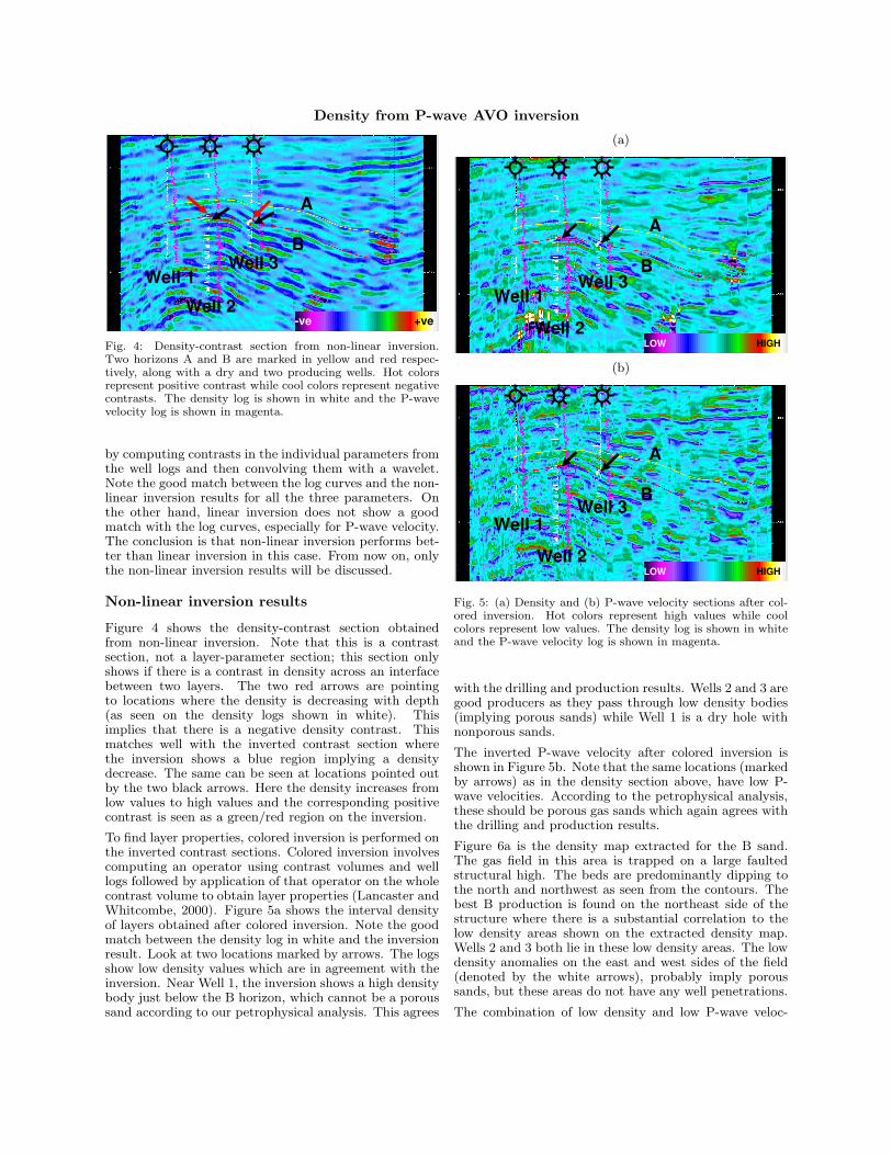
Fig. 4: Density-contrast section from non-linear inversion.Two horizons A and B are marked in yellow and red respec-tively, along with a dry and two producing wells. Hot colorsrepresent positive contrast while cool colors represent negativecontrasts. The density log is shown in white and the P-wavevelocity log is shown in magenta.

by computing contrasts in the individual parameters fromthe well logs and then convolving them with a wavelet.Note the good match between the log curves and the non-linear inversion results for all the three parameters. Onthe other hand, linear inversion does not show a goodmatch with the log curves, especially for P-wave velocity.The conclusion is that non-linear inversion performs bet-ter than linear inversion in this case. From now on, onlythe non-linear inversion results will be discussed.

Non-linear inversion results

Figure 4 shows the density-contrast section obtainedfrom non-linear inversion. Note that this is a contrastsection, not a layer-parameter section; this section onlyshows if there is a contrast in density across an interfacebetween two layers. The two red arrows are pointingto locations where the density is decreasing with depth(as seen on the density logs shown in white). Thisimplies that there is a negative density contrast. Thismatches well with the inverted contrast section wherethe inversion shows a blue region implying a densitydecrease. The same can be seen at locations pointed outby the two black arrows. Here the density increases fromlow values to high values and the corresponding positivecontrast is seen as a green/red region on the inversion.

To find layer properties, colored inversion is performed onthe inverted contrast sections. Colored inversion involvescomputing an operator using contrast volumes and welllogs followed by application of that operator on the wholecontrast volume to obtain layer properties (Lancaster andWhitcombe, 2000). Figure 5a shows the interval densityof layers obtained after colored inversion. Note the goodmatch between the density log in white and the inversionresult. Look at two locations marked by arrows. The logsshow low density values which are in agreement with theinversion. Near Well 1, the inversion shows a high densitybody just below the B horizon, which cannot be a poroussand according to our petrophysical analysis. This agrees

(a)

LOW HIGH

Well 1

Well 2

Well 3B

A

(b)

LOW HIGH

Well 1

Well 2

Well 3B

A

Fig. 5: (a) Density and (b) P-wave velocity sections after col-ored inversion. Hot colors represent high values while coolcolors represent low values. The density log is shown in whiteand the P-wave velocity log is shown in magenta.

with the drilling and production results. Wells 2 and 3 aregood producers as they pass through low density bodies(implying porous sands) while Well 1 is a dry hole withnonporous sands.

The inverted P-wave velocity after colored inversion isshown in Figure 5b. Note that the same locations (markedby arrows) as in the density section above, have low P-wave velocities. According to the petrophysical analysis,these should be porous gas sands which again agrees withthe drilling and production results.

Figure 6a is the density map extracted for the B sand.The gas field in this area is trapped on a large faultedstructural high. The beds are predominantly dipping tothe north and northwest as seen from the contours. Thebest B production is found on the northeast side of thestructure where there is a substantial correlation to thelow density areas shown on the extracted density map.Wells 2 and 3 both lie in these low density areas. The lowdensity anomalies on the east and west sides of the field(denoted by the white arrows), probably imply poroussands, but these areas do not have any well penetrations.

The combination of low density and low P-wave veloc-

Density from P-wave AVO inversion

(a)

HI

Well 1

Well 2

Well 3

G/W

G/W

LOW HIGH

(b)

HI

G/W

G/W

Well 1

Well 2

Well 3

LOW HIGH

Fig. 6: (a) Density and (b) P-wave velocity maps extractedfor B sand. Hot colors represent high values while cool colorsrepresent low values. The contours shown in red denote theapproximate gas/water contact for the B horizon.

ity has the highest probability of being a productive gassand. For the highly productive portion of the B horizon,there are low velocity regions (Figure 6b) which overlielow density regions. The two productive wells (Wells 2and 3) lie in low P-wave velocity regions while the dryhole (Well 1) is in the high P-wave velocity region. Thecumulative production from the B horizon in the Well 2fault block is 57 bcf. The cumulative production in theWell 3 fault block is 139 bcf. This can be contrasted withthe western fault block which has both substantially highdensity and high P-wave velocities; this block has onlyproduced 2.4 bcf of gas. For the low density anomaliesnoted earlier on the east and west sides of the field, thereare no distinct features on the P-wave map. At some loca-tions, the P-wave velocity is high while at others it is low.For this low density and erratic velocity, the fluid proper-ties for these anomalies cannot be accurately determined.

Because these areas are both structurally low to the gas-water contacts in the field, the sands are undoubtedly wethere.

Discussion

Even though density inversion was successful in thisfield, this technique should not be blindly applied toall areas. Care should be taken while interpreting theresults as a mismatch was observed at one well locatedoutside of the field. The well passes through a thick wetsand but inversion results show a high density region.The thick sand zone has many interbedded shales andthus interference of reflections and tuning might beyielding the wrong inversion results. It is also possiblethat this contradictory result may have several otherexplanations: the data might not have been zero-phasedat the well, the inversion might be trapped in a localminima, violation of certain assumptions like absenceof attenuation, anisotropy etc. More analysis needsto be done to understand the cause of this mismatch.The important lesson is to be careful while interpretingresults and geological information and other evidenceshould be taken into account to improve the chances ofsuccess.

Conclusions

Density is the primary driver of reflectivity in this field.Petrophysical analysis suggests that porous gas sandshave low density and low P-wave velocity. Porous sandscan easily be distinguished from shales and tight sands,but separating gas sands from wet sands is more chal-lenging. Because gas sands have higher porosity and thuslower density than other lithologies, density informationcan help in locating them, especially when coupled withother geological and structural data. Density extractedfrom prestack AVO data shows a good match with logand production data and thus AVO inversion for densityworks well. Moreover, non-linear inversion producedbetter results than linear inversion in this case and sothis should be the preferred methodology. The extracteddensity and P-wave velocity helped identify gas sands inthe field as seen from the good correlation between theinterpretation and the log and production data in thefield.

Acknowledgments

We are grateful to BP for permission to publish thispaper. We also thank SEI (Seismic Exchange, Inc.) forproviding the seismic data. The seismic data is owned orcontrolled by Seismic Exhange, Inc.; the interpretation isthat of BP.

Density from P-wave AVO inversion

References

Debski, W., and A. Tarantola, 1995, Information on elas-tic parameters obtained from the amplitudes of re-flected waves: Geophysics, 60, 1426-1436.

Kabir, N., R. Crider, R. Ramkhelawan, and C. Baynes,2006, Can hydrocarbon saturation be estimated us-ing density contrast parameter?: CSEG Recorder,31-37.

Lancaster, S., and D. Whitcombe, 2000, Fast-track ‘col-ored’ inversion: 70th Annual International Meeting,SEG, Expanded Abstracts, 19, 1572-1575.

Lavaud, B., N. Kabir, and G. Chavent, 1999, PushingAVO inversion beyond linearized approximation: J.Seis. Expl., 8, 279-302.

Li, Y., 2005, A study on applicability of density in-version in defining reservoirs: 75th Annual Interna-tional Meeting, SEG, Expanded Abstracts, 24, 1646-1649.

Smith, G., and P. Gidlow, 1987, Weighted stacking forrock property estimation and detection of gas: Geo-physical Prospecting, 35, 993-1014.