1

Dense Subgraph Extraction with Application toCommunity Detection

Jie Chen and Yousef Saad

Abstract— This paper presents a method for identifying aset of dense subgraphs of a given sparse graph. Within themain applications of this “dense subgraph problem”, the densesubgraphs are interpreted as communities, as in, e.g., socialnetworks. The problem of identifying dense subgraphs helpsanalyze graph structures and complex networks and it is knownto be challenging. It bears some similarities with the problemof reordering/blocking matrices in sparse matrix techniques.We exploit this link and adapt the idea of recognizing matrixcolumn similarities, in order to compute a partial clusteringof the vertices in a graph, where each cluster represents adense subgraph. In contrast to existing subgraph extractiontechniques which are based on a complete clustering of the graphnodes, the proposed algorithm takes into account the fact thatnot every participating node in the network needs to belongto a community. Another advantage is that the method doesnot require to specify the number of clusters; this number isusually not known in advance and is difficult to estimate. Thecomputational process is very efficient, and the effectiveness ofthe proposed method is demonstrated in a few real-life examples.

Index Terms— Dense subgraph, social network, community,matrix reordering, hierarchical clustering, partial clustering.

I. INTRODUCTION

A challenging problem in the analysis of graph structures isthe dense subgraph problem, where given a sparse graph,

the objective is to identify a set of meaningful dense subgraphs.This problem has attracted much attention in recent years dueto the increased interest in studying various complex networks,such as the World Wide Web (information network), socialnetworks, and biological networks, etc. The dense subgraphsare often interpreted as “communities” [1]–[4], based on thebasic assumption that a network system consists of a numberof communities, among which the connections are much fewerthan those inside the same community.

The recent data mining literature has seen various techniquesfor approaching this network analysis problem from different as-pects. Because of a potentially wide variety of purposes, differentdefinitions of communities are employed and methods are pro-posed, ranging from partitioning the network to minimize inter-connections between parts [5], [6], to aiming at extracting a largenumber of subgraphs that have a high enough density [7]–[9]. Inaddition to partitioning-based and density-based approaches, alsoseen are techniques that build hierarchical structures [10]–[13],that exploit stochastic block models [14]–[16], and that extractchains of adjacent cliques [17], [18]. It is beyond the scope of thispaper to list the many existing approaches in such an emergingarea. We refer the interested reader to surveys [19]–[21].

The authors are with the Department of Computer Science and Engineer-ing, University of Minnesota at Twin Cities, MN 55455. Email: {jchen,saad}@cs.umn.edu

In this paper, we focus on the methodology of graph partition-ing/clustering, with the goal of obtaining dense partitions/clusters.A broad set of partitioning techniques (spectral based [6], [22],multilevel based [23], [24], and stochastic based [25]) can be used.However, these methods have several drawbacks and issues thatneed to be addressed for the purpose of network analysis and com-munity detection. The first drawback is that in general, the numberk of partitions is a mandatory input parameter, and the partitioningresult is sensitive to the change of k. In most applications, thenumber k is not known a priori. A number of researchers proposedto remedy this difficulty by tracking a goodness measure, such asthe conductance [4] and the modularity [11], of the partitioningas a function of k. However, this remedy may not always bepractical due to the underlying expensive computational cost ofthe algorithm. Second, most of these methods yield a completeclustering of the data. A crucial question when studying humanbehavior and social phenomena is: “Why should every participantbe grouped into some community?” It is natural to consider thatif a node in a network is far away from the rest of the nodes,then excluding this node from the analysis will usually yield moreaccurate results. Therefore, when attempting to discover commu-nities, an incomplete clustering of the network is usually moredesirable. Finally, note that many graph partitioning techniquesbased on optimizing an objective function [26] favor balancing,i.e., sizes of different partitions should not vary too much [5].This may not accurately represent human communities, since itis common for social connections not to be evenly divided.

We propose a dense subgraph extraction approach that ad-dresses the above issues. It is inspired by an effective techniquedesigned for a similar problem—matrix blocking [27], [28]—froma different discipline (solving linear systems). How the proposedapproach overcomes the general drawbacks of graph partitioningmethodology for community detection will be made clear later inthe paper. For now, let us consider the matrix blocking problem,which sheds light on the rationale of the approach we propose forthe graph problem. For solving a linear system, preconditioning(e.g., an incomplete LU factorization) is an important step toimprove the convergence of an iterative method [29], wherebyblocking is a vital ingredient for preconditioning. The mainmotivation is that block preconditioning methods are known toyield better convergence than scalar ones (see [28], [29] andreferences therein). Matrix blocking amounts to symmetricallypermuting the rows and the columns of a sparse matrix such thatthe nonzeros are moved toward the diagonal. In this way, thematrix exhibits dense diagonal blocks, whereas the rest of thearea contains sporadic nonzeros (see Fig. 1(b)). In our case, eachblock naturally corresponds to a dense subgraph, or a communitythat we seek after.

The blocking algorithm presented in [28] groups similarcolumns (and rows) of a matrix according to a cosine similaritymeasure. By a non-trivial adaptation of this algorithm, we obtain

2

what turns out to be a form of a hierarchical clustering (see,e.g. [30] for AGNES and DIANA) of the graph nodes usingthe same similarity measure. Hierarchical structures of a networkhave been exploited for the purpose of community extraction, byperforming either a divisive clustering [11] or an agglomerativeclustering [10], [31]. A feature of our method is that it can beviewed from both perspectives, by using the idea of a similaritygraph G′ computed from the original graph G. In the divisiveperspective edges of G′ are removed in an order of the edgeweights, whereas in the agglomerative perspective edges areinserted to a set of isolated nodes in the opposite order to formG′. This approach avoids tracking/updating all-pairs distances ineach merge or division step in the clustering process. The result isa computationally inexpensive procedure as long as the similarityscores can be efficiently computed.

Before looking at the algorithmic details, we shall mentionhere two important issues concerning this approach. The firstconcerns the similarity measure for building the hierarchy. Be-sides the obvious fact that the matrix blocking technique [28](which inspires the algorithms proposed in this paper) uses thecosine similarity, this measure also has a clear interpretation forcommunities. A large cosine means that two nodes share a largeportion of common neighbors with respect to their own neighborsets, hence it can be interpreted as a probability that the twonodes belong to a community. This measure has been adoptedin mining natural communities [31], and a similar measure—the Jaccard coefficient—is also used for a similar purpose [32].The second is the interpretation of the hierarchy. Traditionalhierarchical clustering methods cut the hierarchy at a specificlevel, yielding a complete partitioning of the graph. However,our goal is to identify dense subgraphs. Therefore, a sensibleapproach is to define the notion of the density, and to walk thehierarchy in a top-down fashion and return clusters only whenthey have high densities. By using this approach, one can navigatethe hierarchy and adjust the density threshold (at almost no timecost) until a desirable result is achieved. Note that by introducingthe definition of density, we do not intend to enumerate all thedense subgraphs; instead, we form an incomplete partitioning ofthe graph with dense partitions.

A common misperception is that computing pairwise similari-ties have at least a quadratic cost, which would make an algorithmbased on such calculations ineffective for large data sets. Thus,to guarantee scalability, the shingling algorithm in [32] (whichemploys the Jaccard coefficient as the similarity measure) mapsthe set of neighbors of each graph node to a small number of“shingles”, and the similarity of the nodes is translated to thenumber of shingles they share. In this paper, we employ a differentapproach. We exploit the fact that the matrix representation of thegraph is sparse, and use sparse matrix computation techniquesto compute the similarities in linear time. In fact, our overallalgorithm is efficient. As will be seen in Sec. III, for a typicalsparse graph, most parts of the algorithm are linear except that inaddition we need to sort an array of size also linear in the numberof graph nodes.

We note that existing community extraction approaches varyconsiderably in terms of applications and properties of the ex-tracted subgraphs (e.g., ones that have the largest densities, thelargest modularities, or bipartite structures, etc), which makesthem difficult to compare, but in general a linear time algorithmequipped with external sorting, such as ours, will be desirable

in facing mega- or giga-scale data. Further, as the study [21]points out, there tend to be a tradeoff between the quality of thesubgraphs and the computational cost for existing methods. Thus,we show in Sec. IV extensive experiments demonstrating that ourresults are accurate and the extracted subgraphs are semanticallymeaningful.

II. DENSE SUBGRAPHS EXTRACTION

Given a sparse graph G(V,E) which consists of the vertexset V and the edge set E, we are interested in identifyingdense subgraphs of G. To be precise, the candidate subgraphsshould have densities higher than a threshold value in order tobe interesting. We consider the following three types of graphs,with an appropriate definition of density for each one.

1) Undirected graphs. Undirected graphs are the most commonmodels of networks, where the directions of the connectionsare unimportant, or can be safely ignored. A natural defi-nition of the graph density is

dG =|E|

|V |(|V | − 1)/2. (1)

Note that dG ∈ [0, 1], and a subgraph has the density oneif and only if it is a clique.

2) Directed graphs. The density of a directed graph is

dG =|E|

|V |(|V | − 1), (2)

since the maximum number of possible directed edgescannot exceed |V |(|V | − 1). In other words, the densityof a directed graph also lies in the range from 0 to 1. Itis interesting to note that if we “undirectify” the graph,i.e., remove the directions of the edges and combine theduplicated resulting edges, we yield an undirected graphG(V, E) with the edge set E. Then,

1

2dG ≤ dG ≤ dG.

An immediate consequence is that if we extract the sub-graphs of the undirected version of the graph given a densitythreshold, we essentially obtain directed subgraphs withdensities at least half of the threshold.

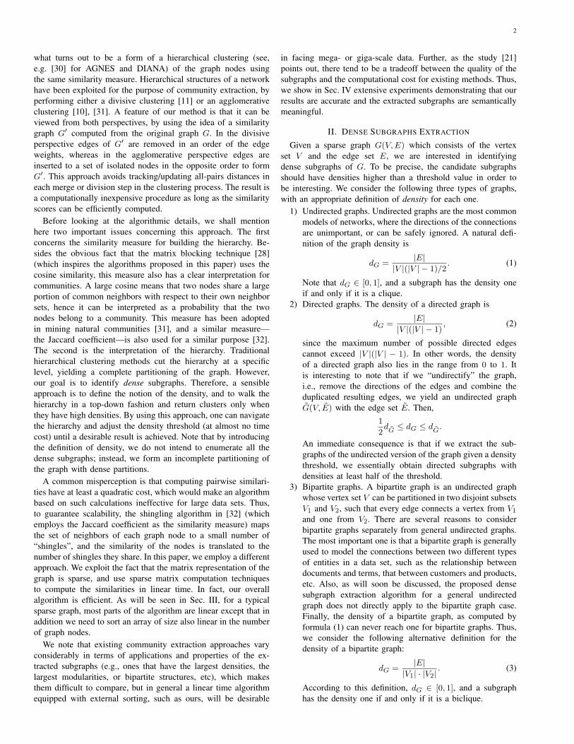
3) Bipartite graphs. A bipartite graph is an undirected graphwhose vertex set V can be partitioned in two disjoint subsetsV1 and V2, such that every edge connects a vertex from V1and one from V2. There are several reasons to considerbipartite graphs separately from general undirected graphs.The most important one is that a bipartite graph is generallyused to model the connections between two different typesof entities in a data set, such as the relationship betweendocuments and terms, that between customers and products,etc. Also, as will soon be discussed, the proposed densesubgraph extraction algorithm for a general undirectedgraph does not directly apply to the bipartite graph case.Finally, the density of a bipartite graph, as computed byformula (1) can never reach one for bipartite graphs. Thus,we consider the following alternative definition for thedensity of a bipartite graph:

dG =|E|

|V1| · |V2|. (3)

According to this definition, dG ∈ [0, 1], and a subgraphhas the density one if and only if it is a biclique.

3

The adjacency matrix A of the above three types of graphshas specific patterns. Throughout the paper, we assume that A issparse, because we are considering subgraphs of a sparse graph.We also assume that the entries of A are either 0 or 1, since theweights of the edges are not taken into account for the densityof a graph. In all cases, the diagonal of A is empty, since wedo not allow self-loops. For undirected graphs, A is symmetric,whereas for directed graphs, A is only square. A natural matrixrepresentation of a bipartite graph is a rectangular matrix B,where B(i, j) is nonzero if and only if there is an edge connectingi ∈ V1 and j ∈ V2. The adjacency matrix for such a bipartite graphis indeed

A =

[0 B

BT 0

],

where the vertices from V1 are ordered before those from V2.Note that there are situations where we do not know that thegiven undirected graph is bipartite in advance, i.e., A is givenin a permuted form where the above 2 × 2 block structure isnot revealed. In such a case, a simple strategy adapted from thebreadth first search can be used to check if the inherent undirectedgraph is bipartite, and if so to extract the two disjoint subsets.

A. Matrix Blocking

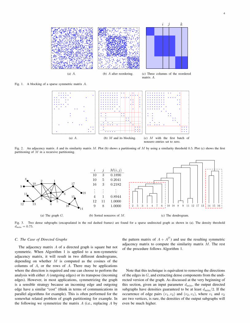
As mentioned earlier, the dense subgraphs extraction methodsproposed in this paper are inspired by the so-called matrixblocking problem. Fig. 1(b) illustrates a blocking result of a sparsematrix A. Here we describe a simple yet effective blocking algo-rithm [28] that accomplishes this result. It exploits the similaritiesbetween a pair of columns in the pattern matrix P of A. Recallthat P is obtained from A by simply replacing its nonzero entriesby ones. The idea is that the nonzero patterns of two columnscorresponding to the same block should be more similar thanthose of the two columns that correspond to different blocks. Tobe specific, let some dense block of the reordered P correspondto a subset of vertices Vs. Also, let i, j ∈ Vs and k /∈ Vs; seeFig. 1(c). The heuristic is that the cosine of the angle betweenthe i-th and the j-th columns of P is large, whereas that of thei-th and the k-th (or the j-th and the k-th) columns is small.The blocking algorithm is to find maximal subsets of V such thatinside the same subset, for each vertex i, there exists a vertexj 6= i such that the cosine of P (:, i) and P (:, j) is larger than apredefined threshold.

The adjacency matrix of an undirected graph plays exactlythe same role as P here. Roughly speaking, the goal of densesubgraph extraction is to reorder the adjacency matrix and tofind the dense diagonal blocks, each of which represents a densesubgraph. One is tempted to directly apply the above algorithmon the adjacency matrix of a given graph. However, a difficultyarises when choosing an appropriate similarity threshold. Afurther concern is that each block should employ a differentthreshold. For example, two columns corresponding to a largerblock have a higher probability of yielding a larger cosine thanthose corresponding to a smaller block.

B. The Case of Undirected Graphs

Consider the matrix M that stores the cosines between any twocolumns of the adjacency matrix A:

M(i, j) =〈A(:, i), A(:, j)〉‖A(:, i)‖ ‖A(:, j)‖ . (4)

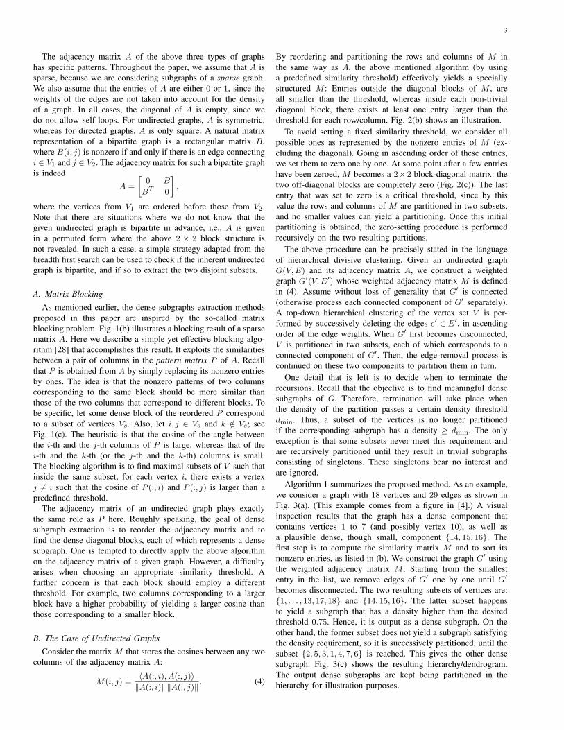
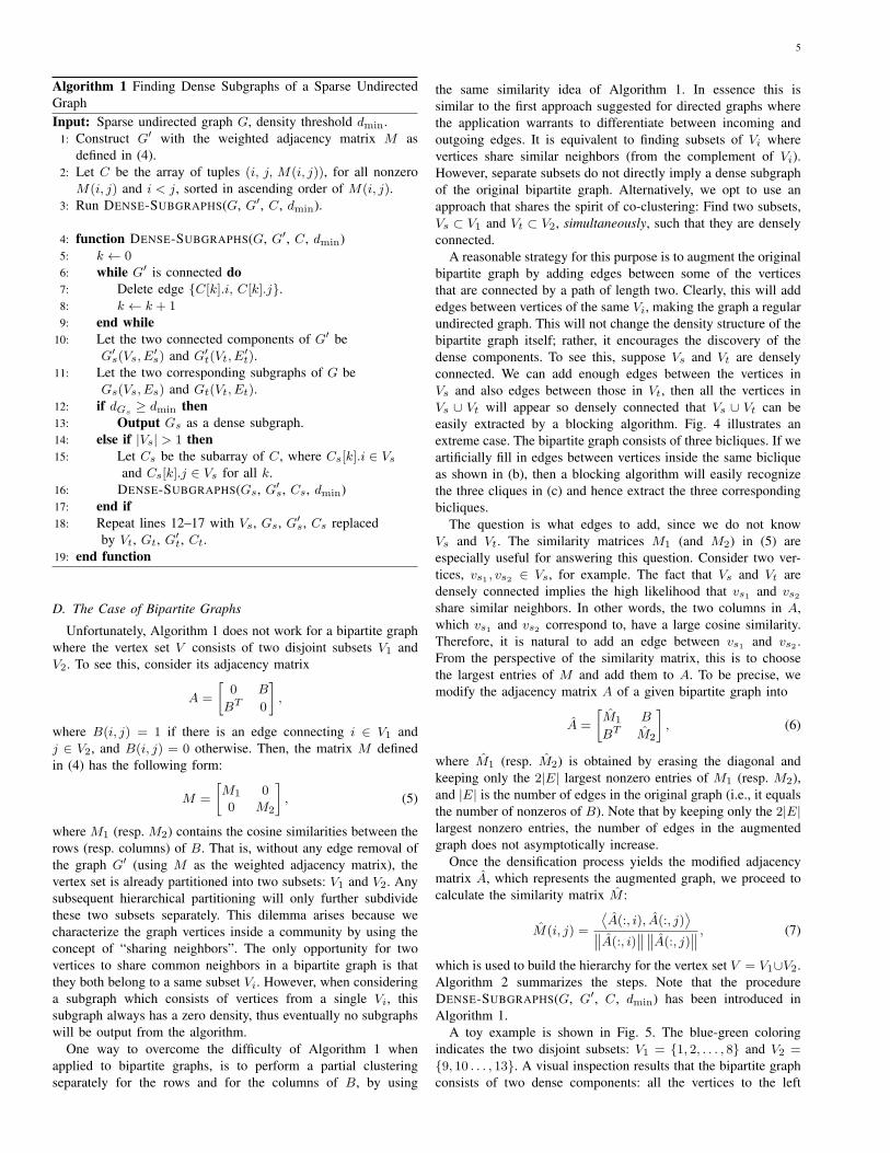
By reordering and partitioning the rows and columns of M inthe same way as A, the above mentioned algorithm (by usinga predefined similarity threshold) effectively yields a speciallystructured M : Entries outside the diagonal blocks of M , areall smaller than the threshold, whereas inside each non-trivialdiagonal block, there exists at least one entry larger than thethreshold for each row/column. Fig. 2(b) shows an illustration.

To avoid setting a fixed similarity threshold, we consider allpossible ones as represented by the nonzero entries of M (ex-cluding the diagonal). Going in ascending order of these entries,we set them to zero one by one. At some point after a few entrieshave been zeroed, M becomes a 2×2 block-diagonal matrix: thetwo off-diagonal blocks are completely zero (Fig. 2(c)). The lastentry that was set to zero is a critical threshold, since by thisvalue the rows and columns of M are partitioned in two subsets,and no smaller values can yield a partitioning. Once this initialpartitioning is obtained, the zero-setting procedure is performedrecursively on the two resulting partitions.

The above procedure can be precisely stated in the languageof hierarchical divisive clustering. Given an undirected graphG(V,E) and its adjacency matrix A, we construct a weightedgraph G′(V,E′) whose weighted adjacency matrix M is definedin (4). Assume without loss of generality that G′ is connected(otherwise process each connected component of G′ separately).A top-down hierarchical clustering of the vertex set V is per-formed by successively deleting the edges e′ ∈ E′, in ascendingorder of the edge weights. When G′ first becomes disconnected,V is partitioned in two subsets, each of which corresponds to aconnected component of G′. Then, the edge-removal process iscontinued on these two components to partition them in turn.

One detail that is left is to decide when to terminate therecursions. Recall that the objective is to find meaningful densesubgraphs of G. Therefore, termination will take place whenthe density of the partition passes a certain density thresholddmin. Thus, a subset of the vertices is no longer partitionedif the corresponding subgraph has a density ≥ dmin. The onlyexception is that some subsets never meet this requirement andare recursively partitioned until they result in trivial subgraphsconsisting of singletons. These singletons bear no interest andare ignored.

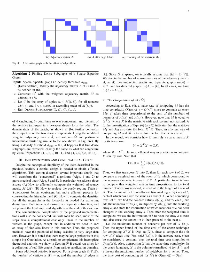
Algorithm 1 summarizes the proposed method. As an example,we consider a graph with 18 vertices and 29 edges as shown inFig. 3(a). (This example comes from a figure in [4].) A visualinspection results that the graph has a dense component thatcontains vertices 1 to 7 (and possibly vertex 10), as well asa plausible dense, though small, component {14, 15, 16}. Thefirst step is to compute the similarity matrix M and to sort itsnonzero entries, as listed in (b). We construct the graph G′ usingthe weighted adjacency matrix M . Starting from the smallestentry in the list, we remove edges of G′ one by one until G′

becomes disconnected. The two resulting subsets of vertices are:{1, . . . , 13, 17, 18} and {14, 15, 16}. The latter subset happensto yield a subgraph that has a density higher than the desiredthreshold 0.75. Hence, it is output as a dense subgraph. On theother hand, the former subset does not yield a subgraph satisfyingthe density requirement, so it is successively partitioned, until thesubset {2, 5, 3, 1, 4, 7, 6} is reached. This gives the other densesubgraph. Fig. 3(c) shows the resulting hierarchy/dendrogram.The output dense subgraphs are kept being partitioned in thehierarchy for illustration purposes.

4

(a) A. (b) A after reordering.

i j k

(c) Three columns of the reorderedmatrix A.

Fig. 1. A blocking of a sparse symmetric matrix A.

(a) A. (b) M and its blocking. (c) M with the first batch ofnonzero entries set to zero.

Fig. 2. An adjacency matrix A and its similarity matrix M . Plot (b) shows a partitioning of M by using a similarity threshold 0.5. Plot (c) shows the firstpartitioning of M in a recursive partitioning.

12

3

45

6

7

8

910

11

12 13

14

15

16

17

18

(a) The graph G.

i j M(i, j)

10 3 0.1890

10 5 0.2041

16 3 0.2182...

......

4 1 0.8944

12 11 1.0000

9 8 1.0000

(b) Sorted nonzeros of M .

2 5 3 1 4 7 6 10 18 8 9 11 12 17 13 14 15 16

(c) The dendrogram.

Fig. 3. Two dense subgraphs (encapsulated in the red dashed frames) are found for a sparse undirected graph as shown in (a). The density thresholddmin = 0.75.

C. The Case of Directed Graphs

The adjacency matrix A of a directed graph is square but notsymmetric. When Algorithm 1 is applied to a non-symmetricadjacency matrix, it will result in two different dendrograms,depending on whether M is computed as the cosines of thecolumns of A, or the rows of A. There may be applicationswhere the direction is required and one can choose to perform theanalysis with either A (outgoing edges) or its transpose (incomingedges). However, in most applications, symmetrizing the graphis a sensible strategy because an incoming edge and outgoingedge have a similar “cost” (think in terms of communications inparallel algorithms for example). This is often performed for thesomewhat related problem of graph partitioning for example. Inthe following we symmetrize the matrix A (i.e., replacing A by

the pattern matrix of A + AT ) and use the resulting symmetricadjacency matrix to compute the similarity matrix M . The restof the procedure follows Algorithm 1.

Note that this technique is equivalent to removing the directionsof the edges in G, and extracting dense components from the undi-rected version of the graph. As discussed at the very beginning ofthis section, given an input parameter dmin, the output directedsubgraphs have densities guaranteed to be at least dmin/2. If theoccurrence of edge pairs (v1, v2) and (v2, v1), where v1 and v2are two vertices, is rare, the densities of the output subgraphs willeven be much higher.

5

Algorithm 1 Finding Dense Subgraphs of a Sparse UndirectedGraphInput: Sparse undirected graph G, density threshold dmin.

1: Construct G′ with the weighted adjacency matrix M asdefined in (4).

2: Let C be the array of tuples (i, j, M(i, j)), for all nonzeroM(i, j) and i < j, sorted in ascending order of M(i, j).

3: Run DENSE-SUBGRAPHS(G, G′, C, dmin).

4: function DENSE-SUBGRAPHS(G, G′, C, dmin)5: k ← 0

6: while G′ is connected do7: Delete edge {C[k].i, C[k].j}.8: k ← k + 1

9: end while10: Let the two connected components of G′ be

G′s(Vs, E

′s) and G′

t(Vt, E′t).

11: Let the two corresponding subgraphs of G beGs(Vs, Es) and Gt(Vt, Et).

12: if dGs≥ dmin then

13: Output Gs as a dense subgraph.14: else if |Vs| > 1 then15: Let Cs be the subarray of C, where Cs[k].i ∈ Vs

and Cs[k].j ∈ Vs for all k.16: DENSE-SUBGRAPHS(Gs, G′

s, Cs, dmin)17: end if18: Repeat lines 12–17 with Vs, Gs, G′

s, Cs replacedby Vt, Gt, G′

t, Ct.19: end function

D. The Case of Bipartite Graphs

Unfortunately, Algorithm 1 does not work for a bipartite graphwhere the vertex set V consists of two disjoint subsets V1 andV2. To see this, consider its adjacency matrix

A =

[0 B

BT 0

],

where B(i, j) = 1 if there is an edge connecting i ∈ V1 andj ∈ V2, and B(i, j) = 0 otherwise. Then, the matrix M definedin (4) has the following form:

M =

[M1 0

0 M2

], (5)

where M1 (resp. M2) contains the cosine similarities between therows (resp. columns) of B. That is, without any edge removal ofthe graph G′ (using M as the weighted adjacency matrix), thevertex set is already partitioned into two subsets: V1 and V2. Anysubsequent hierarchical partitioning will only further subdividethese two subsets separately. This dilemma arises because wecharacterize the graph vertices inside a community by using theconcept of “sharing neighbors”. The only opportunity for twovertices to share common neighbors in a bipartite graph is thatthey both belong to a same subset Vi. However, when consideringa subgraph which consists of vertices from a single Vi, thissubgraph always has a zero density, thus eventually no subgraphswill be output from the algorithm.

One way to overcome the difficulty of Algorithm 1 whenapplied to bipartite graphs, is to perform a partial clusteringseparately for the rows and for the columns of B, by using

the same similarity idea of Algorithm 1. In essence this issimilar to the first approach suggested for directed graphs wherethe application warrants to differentiate between incoming andoutgoing edges. It is equivalent to finding subsets of Vi wherevertices share similar neighbors (from the complement of Vi).However, separate subsets do not directly imply a dense subgraphof the original bipartite graph. Alternatively, we opt to use anapproach that shares the spirit of co-clustering: Find two subsets,Vs ⊂ V1 and Vt ⊂ V2, simultaneously, such that they are denselyconnected.

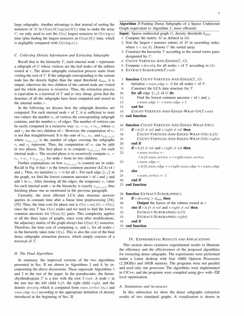
A reasonable strategy for this purpose is to augment the originalbipartite graph by adding edges between some of the verticesthat are connected by a path of length two. Clearly, this will addedges between vertices of the same Vi, making the graph a regularundirected graph. This will not change the density structure of thebipartite graph itself; rather, it encourages the discovery of thedense components. To see this, suppose Vs and Vt are denselyconnected. We can add enough edges between the vertices inVs and also edges between those in Vt, then all the vertices inVs ∪ Vt will appear so densely connected that Vs ∪ Vt can beeasily extracted by a blocking algorithm. Fig. 4 illustrates anextreme case. The bipartite graph consists of three bicliques. If weartificially fill in edges between vertices inside the same bicliqueas shown in (b), then a blocking algorithm will easily recognizethe three cliques in (c) and hence extract the three correspondingbicliques.

The question is what edges to add, since we do not knowVs and Vt. The similarity matrices M1 (and M2) in (5) areespecially useful for answering this question. Consider two ver-tices, vs1 , vs2 ∈ Vs, for example. The fact that Vs and Vt aredensely connected implies the high likelihood that vs1 and vs2share similar neighbors. In other words, the two columns in A,which vs1 and vs2 correspond to, have a large cosine similarity.Therefore, it is natural to add an edge between vs1 and vs2 .From the perspective of the similarity matrix, this is to choosethe largest entries of M and add them to A. To be precise, wemodify the adjacency matrix A of a given bipartite graph into

A =

[M1 B

BT M2

], (6)

where M1 (resp. M2) is obtained by erasing the diagonal andkeeping only the 2|E| largest nonzero entries of M1 (resp. M2),and |E| is the number of edges in the original graph (i.e., it equalsthe number of nonzeros of B). Note that by keeping only the 2|E|largest nonzero entries, the number of edges in the augmentedgraph does not asymptotically increase.

Once the densification process yields the modified adjacencymatrix A, which represents the augmented graph, we proceed tocalculate the similarity matrix M :

M(i, j) =

⟨A(:, i), A(:, j)

⟩∥∥A(:, i)∥∥∥∥A(:, j)

∥∥ , (7)

which is used to build the hierarchy for the vertex set V = V1∪V2.Algorithm 2 summarizes the steps. Note that the procedureDENSE-SUBGRAPHS(G, G′, C, dmin) has been introduced inAlgorithm 1.

A toy example is shown in Fig. 5. The blue-green coloringindicates the two disjoint subsets: V1 = {1, 2, . . . , 8} and V2 =

{9, 10 . . . , 13}. A visual inspection results that the bipartite graphconsists of two dense components: all the vertices to the left

6

(a) Adjacency matrix A. (b) A after edge fill-in. (c) Blocking of the matrix in (b).

Fig. 4. A bipartite graph with the effect of edge fill-in.

Algorithm 2 Finding Dense Subgraphs of a Sparse BipartiteGraphInput: Sparse bipartite graph G, density threshold dmin.

1: [Densification:] Modify the adjacency matrix A of G into A

as defined in (6).2: Construct G′ with the weighted adjacency matrix M as

defined in (7).3: Let C be the array of tuples (i, j, M(i, j)), for all nonzero

M(i, j) and i < j, sorted in ascending order of M(i, j).4: Run DENSE-SUBGRAPHS(G, G′, C, dmin).

of 6 (including 6) contribute to one component, and the rest ofthe vertices (arranged in a hexagon shape) form the other. Thedensification of the graph, as shown in (b), further convincesthe conjecture of the two dense components. Using the modifiedweighted adjacency matrix A, we compute M and perform ahierarchical clustering similar to the one shown in Fig. 3(c). Byusing a density threshold dmin = 0.5, it happens that two densesubgraphs are extracted, exactly the same as what we conjectureby visual inspection: {1, 2, 3, 9, 10, 11} and {4, 5, 6, 7, 8, 12, 13}.

III. IMPLEMENTATION AND COMPUTATIONAL COSTS

Despite the conceptual simplicity of the ideas described in theprevious section, a careful design is needed to obtain efficientalgorithms. This section discusses several important details thatwill transform the “conceptual” algorithms (Algo. 1 and 2) tomore practical ones (Algo. 3 and 4). In particular, we address threeissues: (A) How to efficiently compute the weighted adjacencymatrix M (M ); (B) How to replace the costly routine DENSE-SUBGRAPHS by an equivalent but more efficient process forconstructing the hierarchy; and (C) How to compute the densitiesfor all the subgraphs in the hierarchy as needed for extractingdense ones. Each issue is discussed in a separate subsection, andwe present the final improved algorithms at the end of this section.

The computational complexities of the proposed implementa-tions will also be considered. As will soon be seen, most of thesteps have a computational cost only linear to the number ofvertices in the graph, except that in addition we need to sortan array of size also linear in this number. Thus, the proposedmethods have the potential of being scalable to very large datasets. However, it is noted that there may be large prefactors in thissimple big-O notation. As a result, to complement this incompletetheoretical analysis, we show in Section IV-B actual run times fora collection of real-life graphs from various application domains.

Some additional notation is needed. For a given graph G(V,E),the number of vertices is |V | = n, and the number of edges is

|E|. Since G is sparse, we typically assume that |E| = O(|V |).We denote the number of nonzero entries of the adjacency matrixA, nz(A). For undirected graphs and bipartite graphs nz(A) =

2|E|, and for directed graphs nz(A) = |E|. In all cases, we havenz(A) = O(n).

A. The Computation of M (M )

According to Eqn. (4), a naive way of computing M has thetime complexity O(nz(A)2) = O(n2), since to compute an entryM(i, j) takes time proportional to the sum of the numbers ofnonzeros of A(:, i) and A(:, j). However, note that M is equal toXTX, where X is the matrix A with each column normalized. Afurther investigation of Eqn. (6) (or (5)) indicates that the matricesM1 and M2 also take the form XTX. Thus, an efficient way ofcomputing M and M is to exploit the fact that X is sparse.

In the sequel, we consider how to multiply a sparse matrix X

by its transpose:Y = XTX := ZX,

where Z = XT . The most efficient way in practice is to computeY row by row. Note that

Y (i, :) =∑j

Z(i, j)X(j, :).

Thus, we first transpose X into Z, then for each row i of Z, wecompute a weighted sum of the rows of X which correspond tothe nonzero elements in row i of Z. A particular issue is howto compute this weighted sum in time proportional to the totalnumber of nonzeros involved, instead of to the length of a row ofX. The technique is to pre-allocate two working arrays a and b,each of which has a size the same as a row of X. When computingrow i of Y , we find the nonzero entries Z(i, j), and for each j, weadd the nonzeros of X(j, :) multiplied by Z(i, j) into the workingarray a, and store the information of which locations of a has beenchanged in the working array b. Then after the weighted sum iscomputed, we use the information in b to reset the array a to zeroand also erase the content in b, then proceed to the next i.

Let the maximum number of nonzeros per row of X be p.Then the upper bound of the time cost of the above techniquefor computing XTX is O(p · nz(X)), since to compute the i-throw of Y takes time O(p ·nz(Z(i, :))). In the average case, p canbe considered a constant, thus the total time cost simplifies toO(nz(X)). Also, transposing X has the same time complexity. Inthe graph language, X is the column-normalized A (or AT ), andp means the maximum number of neighbors for a vertex. Thus,the time cost of computing M (or M ) is O(nz(A)) = O(n).

7

1

2

3

4

5

6

7

8

9

10 11

12

13

(a) Bipartite graph G.

1

2

3

4

5

6

7

8

9

10 11

12

13

(b) Densification of G. Weights of the fill-inedges (dashed) have not been shown.

1 11 2 9 3 10 6 5 7 8 4 12 13

(c) The dendrogram constructed from (b).

Fig. 5. Two dense subgraphs (encapsulated in the red dashed frames) are found for a sparse bipartite graph as shown in (a). The density threshold dmin = 0.5.

We should note that the above method is a standard techniqueused for sparse matrix-matrix multiplications (cf. e.g., [29]).Perhaps the only important point to stress here is the fact thatit takes time only linear in n to multiply two sparse matrices,assuming that the maximum number p of nonzeros per row isbounded by a constant. Note that for some real-life graphs thedegree of a vertex may follow a power low distribution, whichmeans that p can become large for large graphs of a givenapplication. It suffices to have one column/row pair of n entriesfor the cost of the product to rise to O(n2) (because the productbecomes dense). Nevertheless, this situation is rare and it isalso rare that p will be O(n), and so the situation where thecomputational cost will rise to the forbidding O(n2) is rare inpractice.

B. The Computation of the Hierarchy/Dendrogram

The routine DENSE-SUBGRAPHS (cf. Algorithm 1) essentiallycomputes a hierarchy of the graph vertices in a top-down fashion.Recursive calls of this routine are very time consuming sincebetween lines 5 and 9, with each removal of an edge in G′, a graphtraversal procedure (such as the breadth first search) is needed toexamine the connectivity of the graph. However, as the two toyexamples (cf. Fig. 3(c) and 5(c)) suggest, it is entirely possibleto build the dendrogram T in an opposite (but equivalent) way:the bottom-up fashion.

The key is the array C which is sorted in ascending order ofthe nonzero entries M(i, j) (or M(i, j))1. It indicates the order ofthe merges in the hierarchy/dendrogram T . Initially, each vertexv ∈ V is a separate tree in the forest. Beginning from the end ofthe array C, each time we have a pair (i, j). We find the rootsri and rj of i and j, respectively. If ri and rj are different, wemake a new root r with the left child ri and the right child rj(see Fig. 6). After iterating the whole array C, a single tree isreturned, which is nothing but T .

Note that the above process is equivalent to monitoring theconnected components of a graph when edges are successivelyinserted (a.k.a. incremental connected components [33]). Initiallywe have a virtual graph with the vertex set V but without edges.When reversely iterating the array C, we merge the two subsets siand sj , which i and j belongs to respectively, if si 6= sj . Finally,a single set, which contains all the vertices in V , is returned.

1To reduce the complication in reading, we thereafter omit the text “(orM )” in this subsection. Readers are reminded that whenever the analysis isapplied to a bipartite graph, all the notions involving M should be replacedby M .

r

ri rj

i j

T

Fig. 6. The dendrogram T as a binary tree. Node r is the lowest commonancestor of i and j, and ri and rj are the children of r.

Therefore, we can utilize the two standard disjoint-set opera-tions SET-FIND and SET-UNION to assist the process of buildingT . When we iterate C and get a pair (i, j) each time, we first doSET-FIND(i) → si and SET-FIND(j) → sj . If si = sj , nothingis done. On the other hand, if si 6= sj , we call SET-UNION tocombine si and sj . Meanwhile, we make a new node r which hasthe ri and rj (stored with the disjoint-set data structure) as thetwo children, and associate r with the combined set s = si ∪ sj .

The total time of the above process can be split in two parts: (a)the time of all the SET-FIND and SET-UNION calls, and (b) thegross time to build T . Part (a) is indeed the incremental connectedcomponent process, which takes time O(n + nz(M)), since thegraph G′ has n vertices and O(nz(M)) edges. Part (b), whichconsists of making new nodes and assigning children, has a timecomplexity linear to the size of T , which is O(n).

We still can improve the performance. Recall that the wholebottom-up process is nothing but to yield the graph G′ from acollection of isolated vertices by successively inserting edges. Wecan stop the insertion of edges at some point. This essentiallyyield an incomplete hierarchy, which is the part of T belowsome level. We opt to stop after we have inserted O(n) edges. Inpractice, the number of inserted edges can be simply set as nz(A),or as τ ·nz(A) by introducing some coefficient parameter τ . Thismay greatly reduce the cost of part (a) from O(n + nz(M)) toO(n), and also some minimal cost of part (b). By doing this, thenegative impact on the final dense subgraphs extraction process ishoped to be minimal, since we only miss, if any, large subgraphsthat have not been formed by merging in the hierarchy. We stillare able to extract the dense parts of the hypothetically missing

8

large subgraphs. Another advantage is that instead of sorting thenonzeros of M in O(nz(M) log(nz(M))) time to make the arrayC, we only need to sort the O(n) largest nonzeros in O(n logn)

time (plus finding the largest nonzeros in O(nz(M)) time, whichis negligible compared with O(n logn).)

C. Collecting Density Information and Extracting Subgraphs

Recall that in the hierarchy T , each internal node r representsa subgraph of G whose vertices are the leaf nodes of the subtreerooted at r. The dense subgraphs extraction process starts fromvisiting the root of T . If the subgraph corresponding to the currentnode has the density higher than the input threshold dmin, it isoutput; otherwise the two children of the current node are visitedand the whole process is recursive. Thus, the extraction processis equivalent to a traversal of T and is very cheap, given that thedensities of all the subgraphs have been computed and stored inthe internal nodes r.

In the following we discuss how the subgraph densities arecomputed. For each internal node r of T , it is sufficient to storetwo values: the number nr of vertices the corresponding subgraphcontains, and the number er of edges. The number of vertices canbe easily computed in a recursive way: nr = nri +nrj , where riand rj are the two children of r. However, the computation of eris not that straightforward. It is the sum of eri , erj and ec(ri,rj),where ec(ri,rj) is the number of edges crossing the subgraphsri and rj represent. Thus, the computation of er can be splitin two phases. The first phase is to compute ec(ri,rj) for eachinternal node r. The second phase is to recursively compute er =

eri + erj + ec(ri,rj) for node r from its two children.Further explanations on how ec(ri,rj) is counted are in order.

Recall in Fig. 6 that r is the lowest common ancestor (LCA) of iand j. Thus, we initialize er = 0 for all r. For each edge {i, j} inthe graph, we find the lowest common ancestor r of i and j andadd 1 to er . After iterating all the edges, the temporary er valuefor each internal node r in the hierarchy is exactly ec(ri,rj), thusfinishing phase one as mentioned in the previous paragraph.

Currently, the most efficient LCA data structure answersqueries in constant time after a linear time preprocessing [34],[35]. Thus, the time cost for phase one is O(n+nz(A)) = O(n),since the tree T has O(n) nodes and we need to find the lowestcommon ancestors for O(nz(A)) pairs. This complexity appliesto all the three types of graphs, since even after modifications,the adjacency matrix of the graph always has O(nz(A)) nonzeros.Therefore, the time cost of computing nr and er for all nodes r

in the hierarchy takes time O(n). This is also the cost of the finaldense subgraphs extraction process, which simply consists of atraversal of T .

D. The Final Algorithms

In summary, the improved versions of the two algorithmspresented in Sec. II are shown in Algorithms 3 and 4, by in-corporating the above discussions. These supersede Algorithms 1and 2 in the rest of the paper. In the pseudocodes, the hierar-chy/dendrogram T is a tree with the root T.root. A node r inthe tree has the left child left, the right child right, and thedensity density which is computed from num vertex (nr) andnum edge (er) according to the appropriate definition of densityintroduced at the beginning of Sec. II.

Algorithm 3 Finding Dense Subgraphs of a Sparse UndirectedGraph (equivalent to Algorithm 1, more efficient)Input: Sparse undirected graph G, density threshold dmin.

1: Compute the matrix M as defined in (4).2: Sort the largest t nonzero entries of M in ascending order,

where t = nz(A). Denote C the sorted array.3: Construct the hierarchy T according to the sorted vertex pairs

designated by C.4: COUNT-VERTICES-AND-EDGES(T , G)5: Compute r.density for all nodes r of T according to (1).6: EXTRACT-SUBGRAPHS(T.root)

7: function COUNT-VERTICES-AND-EDGES(T , G)8: Initialize r.num edge← 0 for all nodes r of T .9: Construct the LCA data structure for T .

10: for all edge {i, j} of G do11: Find the lowest common ancestor r of i and j.12: r.num edge← r.num edge+ 1

13: end for14: COUNT-VERTICES-AND-EDGES-WRAP-UP(T.root)15: end function

16: function COUNT-VERTICES-AND-EDGES-WRAP-UP(r)17: if r.left 6= nil and r.right 6= nil then18: COUNT-VERTICES-AND-EDGES-WRAP-UP(r.left)19: COUNT-VERTICES-AND-EDGES-WRAP-UP(r.right)20: end if21: if r.left 6= nil and r.right 6= nil then22: r.num vertex←

r.left.num vertex+ r.right.num vertex

23: r.num edge←r.left.num edge+ r.right.num edge+ r.num edge

24: else25: r.num vertex← 1

26: end if27: end function

28: function EXTRACT-SUBGRAPHS(r)29: if r.density > dmin then30: Output the leaves of the subtree rooted at r.31: else if r.left 6= nil and r.right 6= nil then32: EXTRACT-SUBGRAPHS(r.left)33: EXTRACT-SUBGRAPHS(r.right)34: end if35: end function

IV. EXPERIMENTAL RESULTS AND APPLICATIONS

This section shows extensive experimental results to illustratethe efficiency and the effectiveness of the proposed algorithmsfor extracting dense subgraphs. The experiments were performedunder a Linux desktop with four AMD Opteron Processors(2.20GHz) and 16GB memory. The programs were not paralleland used only one processor. The algorithms were implementedin C/C++, and the programs were compiled using g++ with -O2level optimization.

A. Simulations and Accuracies

In this subsection we show the dense subgraphs extractionresults of two simulated graphs. A visualization is shown in

9

Algorithm 4 Finding Dense Subgraphs of a Sparse BipartiteGraph (equivalent to Algorithm 2, more efficient)Input: Sparse bipartite graph G, density threshold dmin.

1: [Densification:] Modify the adjacency matrix A of G into A

as defined in (6).2: Compute the matrix M as defined in (7).3: Sort the largest t nonzero entries of M in ascending order,

where t = nz(A). Denote C the sorted array.4: Construct the hierarchy T according to the sorted vertex pairs

designated by C.5: COUNT-VERTICES-AND-EDGES(T , G). [Instead of counting

the number of vertices r.num vertex for each subgraph,count the number of vertices that belong to each partite setfor each subgraph, in a similar way.]

6: Compute r.density for all nodes r of T according to (3).7: EXTRACT-SUBGRAPHS(T.root)

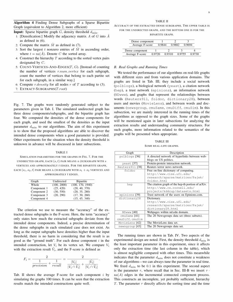
Fig. 7. The graphs were randomly generated subject to theparameters given in Tab. I. The simulated undirected graph hasthree dense components/subgraphs, and the bipartite graph hasfour. We computed the densities of the dense components foreach graph, and used the smallest of the densities as the inputparameter dmin to our algorithms. The aim of this experimentis to show that the proposed algorithms are able to discover theintended dense components when a good parameter is provided.Other experiments for the situation when the density threshold isunknown in advance will be discussed in later subsections.

TABLE ISIMULATION PARAMETERS FOR THE GRAPHS IN FIG. 7. FOR THE

UNDIRECTED GRAPH, EACH (s, t) PAIR MEANS A (SUB)GRAPH WITH s

VERTICES AND APPROXIMATELY t EDGES. FOR THE BIPARTITE GRAPH,EACH (s1, s2, t) PAIR MEANS A (SUB)GRAPH WITH s1 + s2 VERTICES AND

APPROXIMATELY t EDGES.

Graph Undirected BipartiteWhole (100, 2000) (100, 170, 1940)Component 1 (25, 420) (20, 40, 370)Component 2 (30, 550) (20, 35, 280)Component 3 (20, 290) (17, 30, 260)Component 4 (15, 45, 340)

The criterion we use to measure the “accuracy” of the ex-tracted dense subgraphs is the F-score. Here, the term “accuracy”only states how much the extracted subgraphs deviate from theintended dense components. Indeed, a precise determination ofthe dense subgraphs in each simulated case does not exist. Aslong as the output subgraphs have densities higher than the inputthreshold, there is no harm in considering that the result is asgood as the “ground truth”. For each dense component i in theintended construction, let Vi be its vertex set. We compare Viwith the extraction result Vi, and the F-score is defined as

Fi =2

1

precision+

1

recall

=2

|Vi||Vi ∩ Vi|

+|Vi|

|Vi ∩ Vi|

.

Tab. II shows the average F-score for each component i bysimulating the graphs 100 times. It can be seen that the extractionresults match the intended constructions quite well.

TABLE IIACCURACY OF THE EXTRACTED DENSE SUBGRAPHS. THE UPPER TABLE IS

FOR THE UNDIRECTED GRAPH, AND THE BOTTOM ONE IS FOR THE

BIPARTITE GRAPH.

Dense component 1 2 3Average F-score 0.9844 0.9882 0.9694

Dense component 1 2 3 4Average F-score 0.9720 0.9310 0.9755 0.9730

B. Real Graphs and Running Times

We tested the performance of our algorithms on real-life graphswith different sizes and from various application domains. Thegraphs are listed in Tab. III; they include a social network(polblogs), a biological network (yeast), a citation network(hep), a trust network (epinions), an information network(NDwww), and graphs that represent the relationships betweenwords (Reuters911, foldoc, dictionary28), betweenusers and movies (MovieLens), and between words and doc-uments (newsgroup, cmuSame, cmuDiff, cmuSim). In thissubsection, we are mainly interested in the running times of thealgorithms as opposed to the graph sizes. Some of the graphswill be mentioned again in later subsections for analyzing theextraction results and understanding community structures. Forsuch graphs, more information related to the semantics of thegraphs will be presented when appropriate.

TABLE IIISOME REAL-LIFE GRAPHS.

Graph Descriptionpolblogs [36] A directed network of hyperlinks between web-

blogs on US politics.yeast [37] Protein-protein interaction network.

Reuters911 [38] Reuters terror news network.foldoc Free on-line dictionary of computing.

http://www.cise.ufl.edu/research/sparse/matrices/Pajek/foldoc.html

hep The citation graph of the hep-th portion of arXiv.http://www.cs.cornell.edu/projects/kddcup/datasets.html

epinions [39] Trust network of the users on Epinions.com.dictionary28 Dictionary.

http://www.cise.ufl.edu/research/sparse/matrices/Pajek/dictionary28.html

NDwww [40] Webpages within nd.edu domain.cmuSame [41] The 20 Newsgroups data set (three subsets).

cmuDiff, cmuSimMovieLens [42] The MovieLens data set.newsgroup [43] The 20 Newsgroups data set.

The running times are shown in Tab. IV. Two aspects of theexperimental design are noted. First, the density threshold dmin isthe least important parameter in this experiment, since it affectsonly the extraction time (the last column in the table), whichis almost negligible compared with other times. This meanwhileindicates that the parameter dmin does not constitute a weaknessof our algorithms—we can always tune the parameter in real time.We fixed dmin to be 0.1 in this experiment. The second aspectis the parameter τ , where recall that in Sec. III-B we insert τ ·nz(A) edges in the incremental connected component process.This constructs an incomplete, yet probably sufficient, hierarchyT . The parameter τ directly affects the sorting time and the time

10

0 10 20 30 40 50 60 70 80 90 100

0

10

20

30

40

50

60

70

80

90

100

nz = 2000

(a) An undirected graph.

0 10 20 30 40 50 60 70 80 90 100

0

10

20

30

40

50

60

70

80

90

100

nz = 2000

(b) Dense subgraphs of (a).

0 20 40 60 80 100 120 140 160

0

10

20

30

40

50

60

70

80

90

100

nz = 1939

(c) A bipartite graph.

0 20 40 60 80 100 120 140 160

0

10

20

30

40

50

60

70

80

90

100

nz = 1939

(d) Dense subgraphs of (c).

Fig. 7. The extracted dense subgraphs of two simulated graphs.

to compute the hierarchy. In most of the cases τ = 1 is sufficientto yield meaningful dense subgraphs, except that in a few caseswe tune the parameter to an appropriate value such that desirablesubgraphs are extracted. The values of τ are listed in the table.

From Tab. IV we see that the proposed algorithms are efficient.A large part of the running time is spent on the matrix-matrixmultiplication (computing M or M ), which is not difficult toparallelize. Note that all the graphs are run on a single desktopmachine. In the future we will investigate parallel versions of thealgorithms that can deal with massive graphs.

C. Power Law Distribution of the Dense Subgraph Sizes

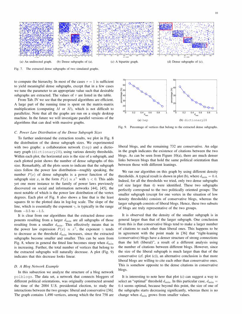
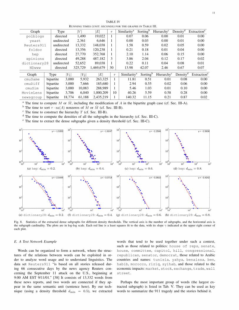
To further understand the extraction results, we plot in Fig. 8the distribution of the dense subgraph sizes. We experimentedwith two graphs: a collaboration network (hep) and a dictio-nary graph (dictionary28), using various density thresholds.Within each plot, the horizontal axis is the size of a subgraph, andeach plotted point shows the number of dense subgraphs of thissize. Remarkably, all the plots seem to indicate that the subgraphsizes follow the power law distribution—roughly speaking, thenumber P (x) of dense subgraphs is a power function of thesubgraph size x, in the form P (x) ∝ xγ with γ < 0. This addsyet one more instance to the family of power laws previouslydiscovered on social and information networks [44], [45], themost notable of which is the power law distribution of the vertexdegrees. Each plot of Fig. 8 also shows a line that is the leastsquares fit to the plotted data in log-log scale. The slope of theline, which is essentially the exponent γ, is typically in the rangefrom −3.5 to −1.5.

It is clear from our algorithms that the extracted dense com-ponents resulting from a larger dmin are all subgraphs of thoseresulting from a smaller dmin. This effectively means that inthe power law expression P (x) ∝ xγ , the exponent γ tendsto decrease as the threshold dmin increases, since the extractedsubgraphs become smaller and smaller. This can be seen fromFig. 8, where in general the fitted line becomes steep when dmin

is increasing. Further, the total number of vertices that belong tothe extracted subgraphs will naturally decrease. A plot (Fig. 9)indicates that this decrease looks linear.

D. A Blog Network Example

In this subsection we analyze the structure of a blog networkpolblogs. The data set, a network that connects bloggers ofdifferent political orientations, was originally constructed aroundthe time of the 2004 U.S. presidential election, to study theinteractions between the two groups: liberal and conservative [36].The graph contains 1,490 vertices, among which the first 758 are

0 0.2 0.4 0.6 0.8 110

20

30

40

50

60

70

dmin

perc

enta

ge (

%)

(a) hep

0 0.2 0.4 0.6 0.8 110

20

30

40

50

dmin

perc

enta

ge (

%)

(b) dictionary28

Fig. 9. Percentage of vertices that belong to the extracted dense subgraphs.

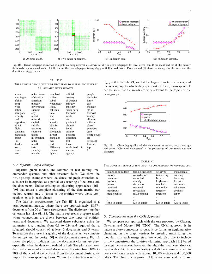
liberal blogs, and the remaining 732 are conservative. An edgein the graph indicates the existence of citations between the twoblogs. As can be seen from Figure 10(a), there are much denserlinks between blogs that hold the same political orientation thanbetween those with different leanings.

We ran our algorithm on this graph by using different densitythresholds. A typical result is shown in plot (b), where dmin = 0.4.Indeed, for all the thresholds we tried, only two dense subgraphs(of size larger than 4) were identified. These two subgraphsperfectly correspond to the two politically oriented groups: Thesmaller subgraph (except for one vertex in the situation of lowdensity thresholds) consists of conservative blogs, whereas thelarger subgraph consists of liberal blogs. Hence, these two subsetsof blogs are truly representative of the two groups.

It is observed that the density of the smaller subgraph is ingeneral larger than that of the larger subgraph. One conclusionfrom this is that conservative blogs tend to make a larger numberof citations to each other than liberal ones. This happens to bein agreement with the point made in [36] that “right-leaning(conservative) blogs have a denser structure of strong connectionsthan the left (liberal)”, a result of a different analysis usingthe number of citations between different blogs. However, sincethe size of the liberal subgraph is much larger than that of theconservative (cf. plot (c)), an alternative conclusion is that moreliberal blogs are willing to cite each other than conservative ones.This is somehow opposite to the dense citations in conservativeblogs.

It is interesting to note here that plot (c) can suggest a way toselect an “optimal” threshold dmin. In this particular case, dmin =

0.4 seems optimal, because beyond this point, the size of one ofthe subgraphs starts decreasing significantly, whereas there is nochange when dmin grows from smaller values.

11

TABLE IVRUNNING TIMES (UNIT: SECONDS) FOR THE GRAPHS IN TABLE III.

Graph Type |V | |E| τ Similaritya Sortingb Hierarchyc Densityd Extractione

polblogs directed 1,490 19,022 1 0.07 0.06 0.00 0.01 0.00yeast undirected 2,361 6,646 1 0.00 0.03 0.00 0.01 0.00

Reuters911 undirected 13,332 148,038 1 1.58 0.59 0.02 0.05 0.00foldoc directed 13,356 120,238 1 0.21 0.18 0.01 0.04 0.00hep directed 27,770 352,768 1 2.10 1.14 0.06 0.15 0.00

epinions directed 49,288 487,182 3 3.86 2.04 0.12 0.17 0.02dictionary28 undirected 52,652 89,038 1 0.22 0.11 0.04 0.08 0.01

NDwww directed 325,729 1,469,679 30 13.98 42.07 2.46 0.67 0.07

Graph Type |V1| |V2| |E| τ Similaritya Sortingb Hierarchyc Densityd Extractione

cmuSame bipartite 3,000 5,932 263,325 1 11.81 0.51 0.01 0.08 0.00cmuDiff bipartite 3,000 7,666 185,680 1 2.94 0.55 0.02 0.06 0.00cmuSim bipartite 3,000 10,083 288,989 1 5.46 1.03 0.01 0.10 0.00

MovieLens bipartite 3,706 6,040 1,000,209 10 40.26 5.59 0.58 0.28 0.00newsgroup bipartite 18,774 61,188 2,435,219 1 140.32 11.15 0.21 0.87 0.02a The time to compute M or M , including the modification of A in the bipartite graph case (cf. Sec. III-A).b The time to sort τ · nz(A) nonzeros of M or M (cf. Sec. III-B).c The time to construct the hierarchy T (cf. Sec. III-B).d The time to compute the densities of all the subgraphs in the hierarchy (cf. Sec. III-C).e The time to extract the dense subgraphs given a density threshold (cf. Sec. III-C).

100

101

102

10310

0

101

102

103

γ = −1.5353

(a) hep: dmin = 0.2.10

010

110

210

3100

101

102

103

γ = −1.9247

(b) hep: dmin = 0.4.10

010

110

210

3100

101

102

103

γ = −2.2506

(c) hep: dmin = 0.6.10

010

110

210

3100

101

102

103

γ = −2.5836

(d) hep: dmin = 0.8.

100

101

10210

0

101

102

103

γ = −2.5444

(e) dictionary28: dmin = 0.2.10

010

110

2100

101

102

103

γ = −3.3714

(f) dictionary28: dmin = 0.4.10

010

110

2100

101

102

103

γ = −3.3915

(g) dictionary28: dmin = 0.6.10

010

110

2100

101

102

103

γ = −3.4242

(h) dictionary28: dmin = 0.8.

Fig. 8. Statistics of the extracted dense subgraphs for different density thresholds. The vertical axis is the number of subgraphs, and the horizontal axis isthe subgraph cardinality. The plots are in log-log scale. Each red line is a least squares fit to the data, with its slope γ indicated at the upper right corner ofeach plot.

E. A Text Network Example

Words can be organized to form a network, where the struc-tures of the relations between words can be exploited in or-der to analyze word usage and to understand linguistics. Thedata set Reuters911 “is based on all stories released dur-ing 66 consecutive days by the news agency Reuters con-cerning the September 11 attack on the U.S., beginning at9:00 AM EST 9/11/01.” [38] It consists of 13,332 words fromthese news reports, and two words are connected if they ap-pear in the same semantic unit (sentence here). By our tech-nique (using a density threshold dmin = 0.5), we extracted

words that tend to be used together under such a context,such as those related to politics: house of reps, senate,house, committee, capitol, hill, congressional,republican, senator, democrat, those related to Arabiccountries and names: tunisia, yahya, benaissa, ben,habib, morocco, riziq, syihab, and those related to theeconomic impacts: market, stock, exchange, trade, wallstreet.

Perhaps the most important group of words (the largest ex-tracted subgraph) is listed in Tab. V. They can be used as keywords to summarize the 911 tragedy and the stories behind it.

12

0 500 1000

0

200

400

600

800

1000

1200

1400

nz = 19022

(a) Original graph.

0 500 1000

0

200

400

600

800

1000

1200

1400

nz = 19022

(b) Two dense subgraphs.

0.2 0.4 0.6 0.8 10

50

100

150

dmin

subg

raph

siz

e

smaller subgraphlarger subgraph

(c) Subgraph size.

0.2 0.4 0.6 0.8 10.2

0.4

0.6

0.8

1

dmin

subg

raph

den

sity

smaller subgraphlarger subgraph

(d) Subgraph density.

Fig. 10. Dense subgraph extraction of a political blog network as shown in (a). Only two subgraphs (of size larger than 4) are identified for all the densitythresholds experimented with. Plot (b) shows the two subgraphs (using dmin = 0.4) in red boxes. Plots (c) and (d) show the changes in the sizes and thedensities as dmin varies.

TABLE VTHE LARGEST GROUP OF WORDS THAT TEND TO APPEAR TOGETHER IN

911-RELATED NEWS REPORTS.

attack united states pres bush official peoplewashington afghanistan taliban country bin ladenafghan american kabul al quaeda forcetroop tuesday wednesday military dayweek government friday thursday mondaynation support pakistan saudi-born strikenew york city time terrorism terroristsecurity report war world sundayraid network new air allianceopposition capital america pakistani militanthijack suicide hijacker aircraft planeflight authority leader bomb pentagonkandahar southern stronghold anthrax casebacterium target airport possible white housegroup information campaign operation jetfbi letter mail test dissidentdeadly month part threat federaltower twin 110-story world trade ctr septstate saturday islamic muslim 11man member fighter agency

F. A Bipartite Graph Example

Bipartite graph models are common in text mining, rec-ommender systems, and other research fields. We show thenewsgroup example where the dense subgraph extraction re-sults can be interpreted as a partial co-clustering of the terms andthe documents. Unlike existing co-clustering approaches [46]–[49] that return a complete clustering of the data matrix, ourmethod returns only a subset of the entities where dense con-nections exist in each cluster.

The data set newsgroup (see Tab. III) is organized as aterm-document matrix, where there are approximately 18,774documents from 20 different newsgroups. The dictionary (numberof terms) has size 61,188. The matrix represents a sparse graphwhere connections are drawn between two types of entities:terms and documents. We extracted dense subgraphs using theparameter dmin ranging from 0.1 to 0.9, and required that asubgraph should consist of at least 5 documents and 3 terms.To measure the clustering quality of the documents, we computethe entropy and the purity [50] of the document clusters. Fig. 11shows the plot. It indicates that the document clusters are pure,especially when the density threshold is high. The plot also showsthe total number of clustered documents. It varies from 10% to30% of the whole document set. From the document clusters, weinspect the corresponding terms. We use the extraction results of

dmin = 0.9. In Tab. VI, we list the largest four term clusters, andthe newsgroup to which they (or most of them) correspond. Itcan be seen that the words are very relevant to the topics of thenewsgroups.

0 0.2 0.4 0.6 0.8 10

0.2

0.4

0.6

0.8

1

dmin

entropypurityclustered documents

Fig. 11. Clustering quality of the documents in newsgroup: entropyand purity. “Clustered documents” is the percentage of documents that areclustered.

TABLE VITHE LARGEST TERM CLUSTERS AND THE CORRESPONDING NEWSGROUPS.

talk.politics.mideast talk.politics.guns sci.crypt misc.forsaleinjuries overwhelmed transfering cruisingcomatose conceded betwen barrelingboyhood crudely keyboards liscencepranks detractors numlock occurancedevalued outraged micronics reknownedmurderous revocation speedier copiousmunicipalities mailbombing phantom loper...

......

...(368 in total) (29 in total) (28 in total) (28 in total)

G. Comparisons with the CNM Approach

We compare our approach with the one proposed by Clauset,Newman and Moore [10] (CNM). The CNM approach is innature a close competitor to ours; it performs an agglomerativeclustering on the graph vertices by greedily maximizing themodularity in each merge step. We would also like to includein the comparisons the divisive clustering approach [11] basedon edge betweenness; however, the algorithm was very slow (atleast with cubic time complexity) and did not terminate withinhours even on a graph with around 10,000 vertices and 100,000edges. Therefore, the approach [11] is not compared here. We

13

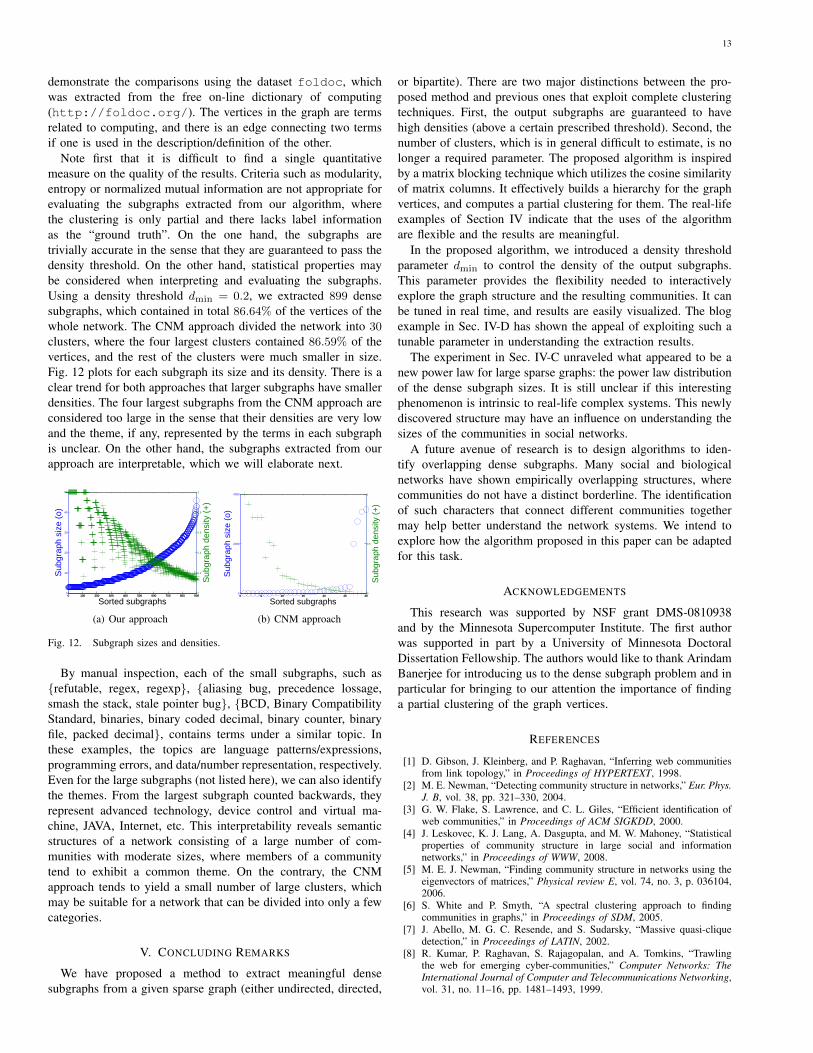
demonstrate the comparisons using the dataset foldoc, whichwas extracted from the free on-line dictionary of computing(http://foldoc.org/). The vertices in the graph are termsrelated to computing, and there is an edge connecting two termsif one is used in the description/definition of the other.

Note first that it is difficult to find a single quantitativemeasure on the quality of the results. Criteria such as modularity,entropy or normalized mutual information are not appropriate forevaluating the subgraphs extracted from our algorithm, wherethe clustering is only partial and there lacks label informationas the “ground truth”. On the one hand, the subgraphs aretrivially accurate in the sense that they are guaranteed to pass thedensity threshold. On the other hand, statistical properties maybe considered when interpreting and evaluating the subgraphs.Using a density threshold dmin = 0.2, we extracted 899 densesubgraphs, which contained in total 86.64% of the vertices of thewhole network. The CNM approach divided the network into 30

clusters, where the four largest clusters contained 86.59% of thevertices, and the rest of the clusters were much smaller in size.Fig. 12 plots for each subgraph its size and its density. There is aclear trend for both approaches that larger subgraphs have smallerdensities. The four largest subgraphs from the CNM approach areconsidered too large in the sense that their densities are very lowand the theme, if any, represented by the terms in each subgraphis unclear. On the other hand, the subgraphs extracted from ourapproach are interpretable, which we will elaborate next.

0 100 200 300 400 500 600 700 800 9000

10

20

30

40

50

Sub

grap

h si

ze (

o)

Sorted subgraphs0 100 200 300 400 500 600 700 800 900

0

0.2

0.4

0.6

0.8

1

Sub

grap

h de

nsity

(+

)

(a) Our approach

0 5 10 15 20 25 300

2000

4000

Sub

grap

h si

ze (

o)

Sorted subgraphs0 5 10 15 20 25 30

0

0.5

1

Sub

grap

h de

nsity

(+

)

(b) CNM approach

Fig. 12. Subgraph sizes and densities.

By manual inspection, each of the small subgraphs, such as{refutable, regex, regexp}, {aliasing bug, precedence lossage,smash the stack, stale pointer bug}, {BCD, Binary CompatibilityStandard, binaries, binary coded decimal, binary counter, binaryfile, packed decimal}, contains terms under a similar topic. Inthese examples, the topics are language patterns/expressions,programming errors, and data/number representation, respectively.Even for the large subgraphs (not listed here), we can also identifythe themes. From the largest subgraph counted backwards, theyrepresent advanced technology, device control and virtual ma-chine, JAVA, Internet, etc. This interpretability reveals semanticstructures of a network consisting of a large number of com-munities with moderate sizes, where members of a communitytend to exhibit a common theme. On the contrary, the CNMapproach tends to yield a small number of large clusters, whichmay be suitable for a network that can be divided into only a fewcategories.

V. CONCLUDING REMARKS

We have proposed a method to extract meaningful densesubgraphs from a given sparse graph (either undirected, directed,

or bipartite). There are two major distinctions between the pro-posed method and previous ones that exploit complete clusteringtechniques. First, the output subgraphs are guaranteed to havehigh densities (above a certain prescribed threshold). Second, thenumber of clusters, which is in general difficult to estimate, is nolonger a required parameter. The proposed algorithm is inspiredby a matrix blocking technique which utilizes the cosine similarityof matrix columns. It effectively builds a hierarchy for the graphvertices, and computes a partial clustering for them. The real-lifeexamples of Section IV indicate that the uses of the algorithmare flexible and the results are meaningful.

In the proposed algorithm, we introduced a density thresholdparameter dmin to control the density of the output subgraphs.This parameter provides the flexibility needed to interactivelyexplore the graph structure and the resulting communities. It canbe tuned in real time, and results are easily visualized. The blogexample in Sec. IV-D has shown the appeal of exploiting such atunable parameter in understanding the extraction results.

The experiment in Sec. IV-C unraveled what appeared to be anew power law for large sparse graphs: the power law distributionof the dense subgraph sizes. It is still unclear if this interestingphenomenon is intrinsic to real-life complex systems. This newlydiscovered structure may have an influence on understanding thesizes of the communities in social networks.

A future avenue of research is to design algorithms to iden-tify overlapping dense subgraphs. Many social and biologicalnetworks have shown empirically overlapping structures, wherecommunities do not have a distinct borderline. The identificationof such characters that connect different communities togethermay help better understand the network systems. We intend toexplore how the algorithm proposed in this paper can be adaptedfor this task.

ACKNOWLEDGEMENTS

This research was supported by NSF grant DMS-0810938and by the Minnesota Supercomputer Institute. The first authorwas supported in part by a University of Minnesota DoctoralDissertation Fellowship. The authors would like to thank ArindamBanerjee for introducing us to the dense subgraph problem and inparticular for bringing to our attention the importance of findinga partial clustering of the graph vertices.

REFERENCES

[1] D. Gibson, J. Kleinberg, and P. Raghavan, “Inferring web communitiesfrom link topology,” in Proceedings of HYPERTEXT, 1998.

[2] M. E. Newman, “Detecting community structure in networks,” Eur. Phys.J. B, vol. 38, pp. 321–330, 2004.

[3] G. W. Flake, S. Lawrence, and C. L. Giles, “Efficient identification ofweb communities,” in Proceedings of ACM SIGKDD, 2000.

[4] J. Leskovec, K. J. Lang, A. Dasgupta, and M. W. Mahoney, “Statisticalproperties of community structure in large social and informationnetworks,” in Proceedings of WWW, 2008.

[5] M. E. J. Newman, “Finding community structure in networks using theeigenvectors of matrices,” Physical review E, vol. 74, no. 3, p. 036104,2006.

[6] S. White and P. Smyth, “A spectral clustering approach to findingcommunities in graphs,” in Proceedings of SDM, 2005.

[7] J. Abello, M. G. C. Resende, and S. Sudarsky, “Massive quasi-cliquedetection,” in Proceedings of LATIN, 2002.

[8] R. Kumar, P. Raghavan, S. Rajagopalan, and A. Tomkins, “Trawlingthe web for emerging cyber-communities,” Computer Networks: TheInternational Journal of Computer and Telecommunications Networking,vol. 31, no. 11–16, pp. 1481–1493, 1999.

14

[9] Y. Dourisboure, F. Geraci, and M. Pellegrini, “Extraction and classi-fication of dense communities in the web,” in Proceedings of WWW,2007.

[10] A. Clauset, M. E. J. Newman, and C. Moore, “Finding communitystructure in very large networks,” Physical review E, vol. 70, no. 6,p. 066111, 2004.

[11] M. E. Newman and M. Girvan, “Finding and evaluating communitystructure in networks,” Physical Review E, vol. 69, no. 2, 2004.

[12] K. Wakita and T. Tsurumi, “Finding community structure in mega-scalesocial networks,” in Proceedings of WWW, 2007.

[13] J. P. Scott, Social Network Analysis: A Handbook, 2nd ed. SagePublications Ltd, 2000.

[14] E. M. Airoldi, D. M. Blei, S. E. Fienberg, and E. P. Xing, “Mixedmembership stochastic blockmodels,” J. Machine Learning Research,vol. 9, no. June, pp. 1981–2014, 2008.

[15] K. Nowicki and T. A. B. Snijders, “Estimation and prediction forstochastic blockstructures,” Journal of the American Statistical Asso-ciation, vol. 96, no. 455, pp. 1077–1087, 2001.

[16] K. Yu, S. Yu, and V. Tresp, “Soft clustering on graphs,” in Proceedingsof NIPS, 2005.

[17] G. Palla, I. Derenyi, I. Farkas, and T. Vicsek, “Uncovering the overlap-ping community structure of complex networks in nature and society,”Nature, vol. 435, no. 7043, pp. 814–818, 2005.

[18] I. Derenyi, G. Palla, and T. Vicsek, “Clique percolation in randomnetworks,” Physical Review Letters, vol. 94, no. 16, 2005.

[19] L. Tang and H. Liu, “Graph mining applications to social networkanalysis,” in Managing and Mining Graph Data (Advances in DatabaseSystems), C. C. Aggarwal and H. Wang, Eds., 2010.

[20] V. E. Lee, N. Ruan, R. Jin, and C. Aggarwal, “A survey of algorithmsfor dense subgraph discovery,” in Managing and Mining Graph Data(Advances in Database Systems), C. C. Aggarwal and H. Wang, Eds.,2010.

[21] L. Danon, A. Dıaz-Guilera, J. Duch, and A. Arenas, “Comparingcommunity structure identification,” Journal of Statistical Mechanics:Theory and Experiment, vol. 2005, p. P09008, 2005.

[22] J. Shi and J. Malik, “Normalized cuts and image segmentation,” IEEETrans. Pattern Anal. Machine Intell., vol. 22, no. 8, pp. 888–905, 2000.

[23] G. Karypis and V. Kumar, “Multilevel k-way partitioning scheme forirregular graphs,” J. Parallel Distrib. Comput., vol. 48, no. 1, pp. 96–129, 1998.

[24] A. Abou-Rjeili and G. Karypis, “Multilevel algorithms for partitioningpower-law graphs,” in Proceedings of IPDPS, 2006.

[25] S. V. Dongen, “Graph clustering via a discrete uncoupling process,”SIAM J. Matrix Anal. Appl., vol. 30, no. 1, pp. 121–141, 2008.

[26] D. S. Hochbaum, “Polynomial time algorithms for ratio regions and avariant of normalized cut,” IEEE Trans. Pattern Anal. Machine Intell.,vol. 32, no. 5, pp. 889–898, 2010.

[27] J. O’Neil and D. B. Szyld, “A block ordering method for sparsematrices,” SIAM J. Sci. Comput., vol. 11, no. 5, pp. 811–823, 1990.

[28] Y. Saad, “Finding exact and approximate block structures for ILUpreconditioning,” SIAM J. Sci. Comput., vol. 24, no. 4, pp. 1107–1123,2002.

[29] ——, Iterative methods for sparse linear systems, 2nd ed. SIAM, 2003.[30] L. Kaufman and P. J. Rousseeuw, Finding Groups in Data: An Intro-

duction to Cluster Analysis. John Wiley & Sons Ltd., 1990.[31] J. Hopcroft, O. Khan, B. Kulis, and B. Selman, “Natural communities

in large linked networks,” in Proceedings of ACM SIGKDD, 2003.[32] D. Gibson, R. Kumar, and A. Tomkins, “Discovering large dense

subgraphs in massive graphs,” in Proceedings of VLDB, 2005.[33] D. Eppstein, Z. Galil, and G. F. Italiano, “Dynamic graph algorithms,” in

CRC Handbook of Algorithms and Theory of Computation, 1997, ch. 22.[34] D. Harel and R. E. Tarjan, “Fast algorithms for finding nearest common

ancestors,” SIAM J. Comput., vol. 13, no. 2, pp. 338–355, 1984.[35] M. A. Bender and M. Farach-Colton, “The LCA problem revisited,” in

Lecture Notes in Computer Science. Springer Berlin/Heidelberg, 2000,pp. 88–94.

[36] L. A. Adamic and N. Glance, “The political blogosphere and the 2004u.s. election: divided they blog,” in Proceedings of LinkKDD, 2005.

[37] D. Bu, Y. Zhao, L. Cai, H. Xue, X. Zhu, H. Lu, J. Zhang, S. Sun,L. Ling, N. Zhang, G. Li, and R. Chen, “Topological structure analysisof the protein-protein interaction network in budding yeast,” Nucl. AcidsRes., vol. 31, no. 9, pp. 2443–2450, 2003.

[38] S. R. Corman, T. Kuhn, R. D. McPhee, and K. J. Dooley, “Studyingcomplex discursive systems: Centering resonance analysis of communi-cation,” Human Communication Research, vol. 28, no. 2, pp. 157–206,2002.

[39] P. Massa and P. Avesani, “Trust-aware recommender systems,” inProceedings of RecSys, 2007.

[40] R. Albert, H. Jeong, and A. L. Barabasi, “The diameter of the worldwide web,” Nature, vol. 401, pp. 130–131, 1999.

[41] A. Banerjee, I. Dhillon, J. Ghosh, and S. Sra, “Clustering on the unithypersphere using von mises-fisher distributions,” J. Machine LearningResearch, vol. 6, pp. 1345–1382, 2005.

[42] J. L. Herlocker, J. A. Konstan, A. Borchers, and J. Riedl, “An algorithmicframework for performing collaborative filtering,” in Proceedings ofSIGIR, 1999.

[43] K. Lang, “Newsweeder: Learning to filter netnews,” in Proceedings ofICML, 1995.

[44] M. Faloutsos, P. Faloutsos, and C. Faloutsos, “On power-law relation-ships of the internet topology,” in Proceedings of SIGCOMM, 1999.

[45] A.-L. Barabasi and R. Albert, “Emergence of scaling in random net-works,” Science, vol. 286, no. 5439, pp. 509–512, 1999.

[46] I. S. Dhillon, “Co-clustering documents and words using bipartitespectral graph partitioning,” in Proceedings of ACM SIGKDD, 2001.

[47] I. S. Dhillon, S. Mallela, and D. S. Modha, “Information-theoretic co-clustering,” in Proceedings of ACM SIGKDD, 2003.

[48] M. Rege, M. Dong, and F. Fotouhi, “Co-clustering documents andwords using bipartite isoperimetric graph partitioning,” in Proceedingsof ICDM, 2006.

[49] A. Banerjee, I. Dhillon, J. Ghosh, S. Merugu, and D. S. Modha, “Ageneralized maximum entropy approach to Bregman co-clustering andmatrix approximation,” J. Machine Learning Research, vol. 8, pp. 1919–1986, 2007.

[50] Y. Zhao and G. Karypis, “Empirical and theoretical comparisons ofselected criterion functions for document clustering,” Machine Learning,vol. 55, no. 3, pp. 311–331, 2004.