Max-Planck-Institut für demografische ForschungMax Planck Institute for Demographic ResearchDoberaner Strasse 114 · D-18057 Rostock · GERMANYTel +49 (0) 3 81 20 81 - 0; Fax +49 (0) 3 81 20 81 - 202; http://www.demogr.mpg.de

This working paper has been approved for release by: Alexia Fürnkranz-Prskawetz(fuernkranz@demogr.mpg.de), Head of the Research Group on Population, Economy, and Environment.

© Copyright is held by the authors.

Working papers of the Max Planck Institute for Demographic Research receive only limited review. Views or opinions expressed in working papers are attributable to the authors and do not necessarily reflect those of the Institute.

Demographic Dynamics andSustainability: Insights from an Integrated, Multi-country Simulation Model

MPIDR WORKING PAPER WP 2002-039AUGUST 2002

Brantley Liddle (btliddle@alum.mit.edu)

Demographic Dynamics and Sustainability: Insights from an Integrated, Multi-country

Simulation Model

Brantley LiddleMPI for Demographic ResearchDoberanerstr. 11418057 Rostock, Germany

btliddle@alum.mit.eduphone: + 49 (0) 381 2081 175fax: + 49 (0) 381 2081 475

ABSTRACT

We develop a simulation model to assess sustainable development on three levels: economic (by

determining production, consumption, investment, direct foreign investment, technology transfer,

and international trade), social (by calculating population change, migration flows, and welfare),

and environmental (by computing the difference between pollution and remediation). The model

follows “representative” countries that differ in their initial endowments (i.e., natural resource

endowment, physical and human capital, technology, and population), and thus in their

development levels and prospects. In a world with movement of goods, people, and capital, free

substitution in production, flexible economic structures, and the ability to upgrade input factors

via investment, we find that, rather than the physical capacity of the earth being responsible for

unsustainable paths, the initial disparities in circumstances among countries and the complex of

internal and international human interrelationships can lead to a “social non sustainability” or

continued divergence of outcomes. In our model history matters (the exogenous history implied

by different starting conditions as well as the endogenous history that evolves over the

simulations) in the ultimate prospects of countries and how they respond to institutions (e.g., free

trade). Many of the most important country-specific starting points relate to population: human

capital and population size, structure, and rates of change.

DisclaimerThe views expressed in this paper are the author’s own views and do not necessarily representthose of the Max Plank Institute for Demographic Research.

2

1. Introduction and Background

Much of the population debate has been couched in the distinctions made by “population

pessimists” and “population optimists.” Population pessimists believe that rapid population

growth will overwhelm any induced response by technological progress and capital accumulation

(Coal and Hoover, 1958 and Ehrlich, 1968). In addition, high youth-dependency, they believe,

raises the requirements for consumption at the expense of savings. Following the logic of the

familiar “IPAT” identity—where I is environmental impact, P is population, A is affluence or

consumption per capita, and T is impact per unit of consumption—pessimists argue that more

people necessarily result in more human impact on the environment. In general pessimistic

models focus on the short to medium run, do not consider feedbacks like substitution in the face

of population pressures, and omit possible positive impacts of population like scale economies.

Population optimists believe that rapid population growth allows countries to capture economies

of scale and promotes technological innovation, either because population pressure or scarcity

induces technological progress (Boserup, 1981), or because more people mean more good ideas

(Simon, 1981). The optimists focus on the longer run and stress the importance of feedbacks,

particularly price induced substitutions.

More recently, a “revisionist position” has emerged. Kelley (2001) defines revisionism

not by its conclusions—revisionists typically argue that most developing countries would benefit

from slower population growth—but by its methods, that is highlighting “… the intermediate to

longer run, taking into account both direct and indirect impacts, and feedbacks within economic,

political, and social systems.” This new literature argues that the growth of the working-aged

population is good for economic growth while growth of young, dependant population is not. In

3

other words, the demographic transition (from high fertility and mortality to low fertility and

mortality) will be first a “burden,” as the youth cohorts increase, but then a “gift,” as the middle,

working aged cohorts swell, and lastly, perhaps, a burden again as aging progresses causing the

retired cohorts to rise. Revisionists concerned with the environment criticize the IPAT framework

for failing to capture interdependencies among P, A, and T.

Much recent, interdisciplinary research has focused on aspects of the economic-

population-environment system. Yet, many of these studies focus on only two of the three

important subsystems. In addition, studies often consider only one or more developed countries

or one or more developing countries, and ignore interactions among levels of development.

Lastly, when studies do consider both developed and developing countries, they usually involve

cross-sectional analysis, and thus, the studies assume transitions or transformations, rather than

directly model or observe them. The simulation modeling technique, in theory, can address the

above shortcomings by building complete, multi-country dynamic models and running them over

long horizons. In addition, as Simon (1977) argues, simulation allows one “to compare the results

of population growth structures [or other variable structures of interest] that have not existed.”

Many simulation models, however, suffer from some combination (of more than one) of

no environment, not multi-country, no endogenous growth, and no developed-developing country

interactions (see reviews by Sanderson, 1980 & 1992; Dellink, 1999; and Loschel, 2002). Bloom

and Canning (2001) argue that models dealing with the “new” demography—emphasizing age-

structure effects rather than total population—should necessarily use a systems framework. Yet,

their own model, which does not include environment, is currently at only the schematic level.

Other population revisionists that use simulation models (e.g., Williamson and Higgins, 2001 and

Lee et al., 2001) developed models that are at most partial equilibrium models and are used to

4

project variables like the savings rate, rather than to account for feedbacks or interrelationships at

multiple levels of a complex, integrated system.

We develop a simulation model, borrowing from economics, demography, and

environmental and political science, to simultaneously consider environment, economic

development, and population/politics by focusing specifically on the impact of important flows

(i.e., pollution, capital, technology, production goods, natural resources, and people). The model

can assess sustainable development on three levels: economic (by determining production,

consumption, investment, direct foreign investment, foreign aid, technology transfer, and

international trade), social (by calculating population growth/change, migration flows, and

political stress levels), and environmental (by calculating natural resource use and the difference

between environmental pollution and upgrading expenditures). The model follows

“representative” countries that differ in their initial endowments (i.e., natural resource

endowment, physical and human capital, technology, and population), and thus in their

development levels and prospects. We take a revisionist tract by focusing on age structure and

transition dynamics. Our model allows us to consider population’s impact on per capita

consumption as well as the social interdependencies among these variables.

In this paper we focus on the impact of demographic dynamics on sustainability

prospects. Specifically, we examine the importance of international migration among countries

with different starting points, and review various population policies for aging, rich countries and

high population growth, poor ones. The following two sections describe the simulation model:

first, a general overview is presented, and the “countries” used in the model are defined; next, the

basic modules are described. Some results from the base case are discussed in Section 4,

focussing particularly on the source of long-run economic growth in the model. Section 5

5

discusses the impact of international migration on rich and middle countries, while section 6

reports the results of population motivated polices in rich and poor countries. Section 7

concludes the paper with a summary of the findings. In addition, an appendix contains some of

the important model equations.

2. Overview of Model

The model contains the following major segments: (1) a global economic system,

covering seven significantly different “countries”; (2) an environmental natural resource system,

relating environmental quality and natural resource capacity to welfare and economic production

and consumption; and (3) induced changes in population growth and age distribution in each

country (including international migration). The economic system comprises sets of relationships

in different stages for each country: (1) production of three kinds of commodities (two final

goods and one intermediate); (2) patterns of international trade and foreign direct investment; (3)

determination of consumption and investment; (4) allocation of investment resources over five

investment categories (physical capital, human capital, natural resource capacity, environmental

quality upgrading, and development of new technology).

There are four types of decision-makers in the model: (1) all consumers; (2) owners of

productive resources, i.e., workers and owners of physical capital and land (or the firms); (3) in

each of seven countries, three separate production sectors (thus making 21 individual “firms”

overall); and (4) an aggregate national “investor” for each country. The aggregate national

investor allocates a country’s total investment pool among different types of investment, actually

engages all those investment activities, determines the size of the total investment pool via a

Keynesian investment function, and determines the market goods-environmental quality tradeoff

(by choosing to spend on environmental quality upgrading).

6

Each type of decision-maker renders decisions via optimization. Consumers choose their

consumption mix (between two final goods) to maximize their utility, derived from demand

functions. The national optimal consumption mix is based on national utility maximization

reflected in consumer goods demand. Since we have no interest in specific consumption

preferences, we assume these demand functions all have unitary price and income elasticities;

thus, budgetary allocations to these goods are constant and, for simplicity, are equal for the two

goods in all countries. Each “industry firm” maximizes its profits. Since there is no leisure or

operation-related depreciation, factor owners maximize period returns to their assets by supplying

what is demanded. The national investor maximizes present discounted value of all investments

performed in each period, based on the marginal productivity of different investment types and

on national preference tradeoffs between market goods and environmental quality. Each type of

investment generates a lifetime marginal value productivity, via sectoral production functions and

profit-maximizing levels of output, which are transformed into present discounted values via a

single social rate of discount specified for each country as a function of its per capita GDP.

Relative rates of return form the basis of allocation. The size of the investment pool is given by a

Keynesian consumption-investment function, modified by social provision for rates of population

dependency.

The model sequentially, deterministically, and in discrete-time runs through (i) equilibria

(individual country labor markets and internationally traded goods), (ii) optimizations (profit

maximization, final goods consumption mix, and investment mix—including welfare-

maximizing goods consumption versus environmental quality choice), and (iii) updates

(productive endowments, discount rates, and population—number, age structure, and mortality

and fertility rates). Thus, at the end (and as a result) of this sequence of events, each country has

7

a new set of input endowments and prices. In addition, there is a new set of international trade

prices. In this manner the whole global system will generate 90-100-period (or year) national

trajectories1.

The country initial conditions are based on judgmental stereotypes of Rich, Middle, and

Poor countries, as enhanced by empirical data on country factor endowments; however, only the

age structure and birth and death rates are taken directly from the empirical data of specific

countries (from Keyfitz and Flieger, 1990). Since the different levels of development or per

capita GDP (in our model and empirically) are essentially defined in terms of technology, human

capital, and physical capital per capita, differences within each level of development refer to

population size and resource (land) endowment. Middle countries differ as well in population

growth rates.

So, there are two Rich countries, one with larger total population and higher resource

endowment per capita; three Middle countries, varying in population, resource base, and

population growth; and two Poor countries, differing in population size. The two Poor countries

have the greatest resource endowment, followed by Middle3, then Middle2 and Rich2; Middle1

and Rich1 have the smallest resource endowment. The Rich countries’ populations have low

birth rates and advanced age structures (based on the European Community circa 1980). The

three Middle countries use data from Venezuela in 1975, Chile in 1980, and Taiwan in 1985, and

thus, vary in the degree to which they have undergone demographic transition. The Poor

1 To calibrate and test the limits of the entire model a series of nested, two-level, full and fractional factorial

experimental designs were used. Factorial designs (described in detail in Schmidt and Launsby, 1992) allow study of

the effects of changes in levels of independent factors as well as of interaction effects. In general, our model’s

behavior is not sensitive even to reasonably large changes in parameters—there is numerical sensitivity to changes in

some parameters; however, behavior robustness is most important for our findings.

8

countries have high birth rates and young age structures (initial data from Guatemala in 1985).

Table 1 shows the most important initial country endowments (these data—with the exception of

TFRs and dependency ratios—as well as the simulation output, are “stylized” and in generic units

applicable to the specific variables they describe, e.g., units of physical capital, production,

consumption, etc.).

Place Table 1 here

3. Model Modules

3.1 Production module

In each country, there are three production sectors: resource intensive industry (producing

a final good), resource nonintensive (“service”) industry (producing a final good), and natural

resource extraction industry (producing an intermediate good). Final goods and processed natural

resources are tradables, so their prices are the same for all countries; wage and rent rates are

determined locally. Because labor (but not capital) is completely mobile (within each country),

countries can shift production each period for competitive advantage. Since the producers are

treated as profit-maximizing price takers, and since physical capital is not sectorally mobile, the

amount of each good produced by each country is a straight-forward optimization calculation.

The local wage rate for each country clears the labor market each period. At the end of each

period each country's rent rate on physical capital is updated by recalculating the average

marginal value product of capital for the three sectors, weighted by the total amount of capital in

each sector. Lastly, world prices for the two final consumption goods and the intermediate,

natural resource good are calculated for use in the following period. These prices are calculated

iteratively by equating forecasted world supply and demand. This (arguably simplified) solution

method results in actual global supplies and demands that equate within +/- one percent (after an

9

initialization process taking from three to seven periods). The national aggregate adjustments in

equilibrium have many lags, constraints, and uncertainties, making for varied speeds of

adjustment. These adjustments are too complex to model simultaneously, so we simplify by

adjusting prices at the end of each period, and leaving the direction of behavioral adjustments to

these new prices to the next period. Adjustments, therefore, lead to continued temporal

changes—a main focus in the model.

The production functions for the two final consumer goods sectors are of “Barro” form.

The production function for the resource extraction sector is slightly different in that we include a

drag parameter to allow for heavy recent production to increase rapidly the cost of further

extraction. This increasing cost to extract can lead to increasing prices for the natural resource,

despite its inexhaustibility. All the production functions are assumed to have constant returns to

scale. The resource intensive industry is less labor intensive than the resource nonintensive one.

The equations as well as the exponents used (see Table A-1) are shown in the appendix.

3.2 Investment module

The share of a country’s total GDP allocated for investment depends positively on the

country’s per capita GDP relative to the initial per capita GDP of the richest country (a measure

of a minimum consumption necessity), and negatively on the country’s young (ages 0-14) and

aged (65+) dependency (i.e., the ratio of those cohorts to the total population). This relationship

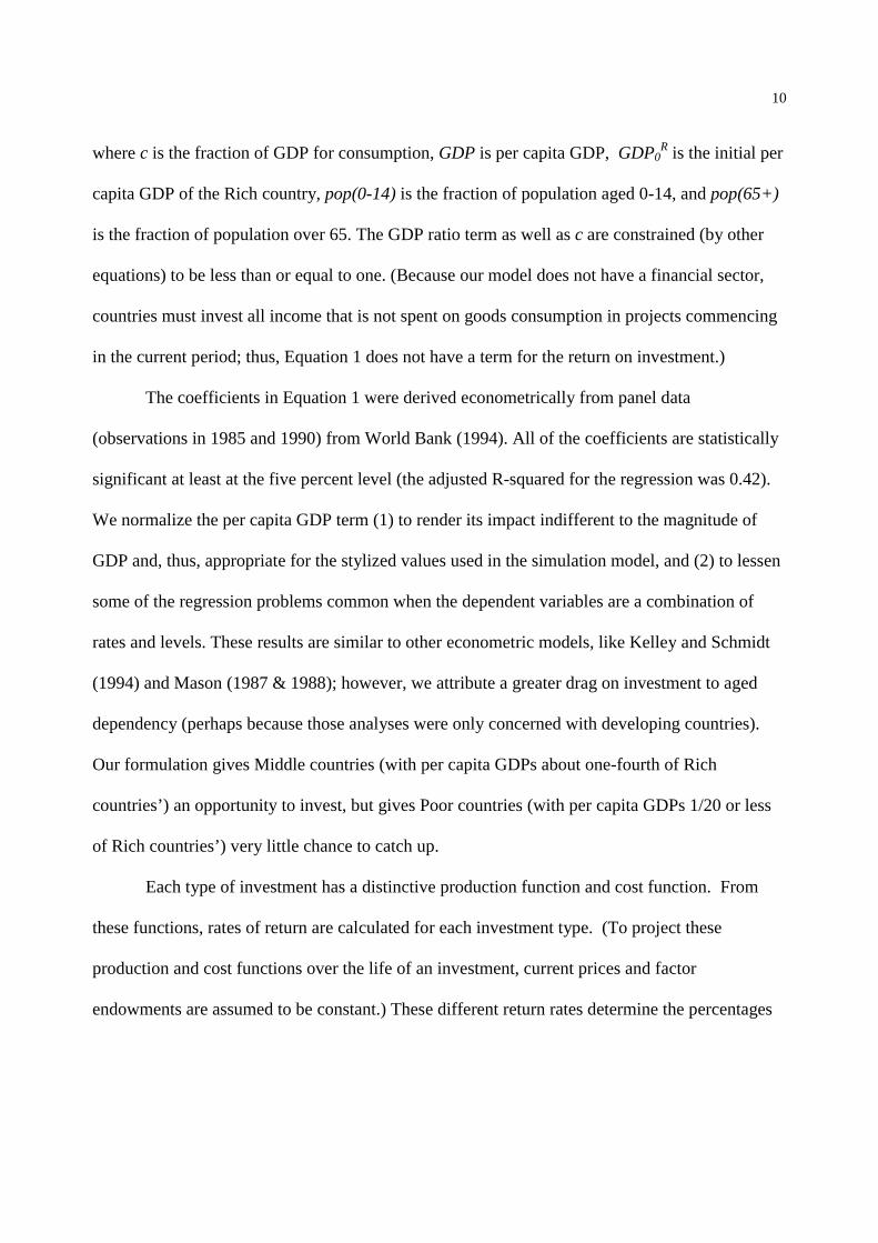
is one of the most important in the model2:

c = 0.34 + -0.071 ln(GDP/ GDP0R) + 0.7 x pop(0-14) + 2.1 x pop(65+) (1)

2 The one exception to the model’s lack of behavioral sensitivity occurs when the coefficients in Equation 1 are

adjusted (by one standard deviation from their econometrically derived values) in the way that constrains investment

the most. Under this scenario the rich countries’ per capita GDP displays "growth and then collapse," as their share of

income for investment eventually reaches zero (driven by their population aging).

10

where c is the fraction of GDP for consumption, GDP is per capita GDP, GDP0R is the initial per

capita GDP of the Rich country, pop(0-14) is the fraction of population aged 0-14, and pop(65+)

is the fraction of population over 65. The GDP ratio term as well as c are constrained (by other

equations) to be less than or equal to one. (Because our model does not have a financial sector,

countries must invest all income that is not spent on goods consumption in projects commencing

in the current period; thus, Equation 1 does not have a term for the return on investment.)

The coefficients in Equation 1 were derived econometrically from panel data

(observations in 1985 and 1990) from World Bank (1994). All of the coefficients are statistically

significant at least at the five percent level (the adjusted R-squared for the regression was 0.42).

We normalize the per capita GDP term (1) to render its impact indifferent to the magnitude of

GDP and, thus, appropriate for the stylized values used in the simulation model, and (2) to lessen

some of the regression problems common when the dependent variables are a combination of

rates and levels. These results are similar to other econometric models, like Kelley and Schmidt

(1994) and Mason (1987 & 1988); however, we attribute a greater drag on investment to aged

dependency (perhaps because those analyses were only concerned with developing countries).

Our formulation gives Middle countries (with per capita GDPs about one-fourth of Rich

countries’) an opportunity to invest, but gives Poor countries (with per capita GDPs 1/20 or less

of Rich countries’) very little chance to catch up.

Each type of investment has a distinctive production function and cost function. From

these functions, rates of return are calculated for each investment type. (To project these

production and cost functions over the life of an investment, current prices and factor

endowments are assumed to be constant.) These different return rates determine the percentages

11

of the total investment pool that are allocated to each investment type via a logit share equation

(thus, investment funds are allocated in proportion to their relative returns).

Each production sector has its own (well-mixed) physical capital allotment, which is

increased through investment and decreased by depreciation (set at five percent a year). Physical

capital created (by investment) at the end of one period is considered operational (included in the

production function) in the following period. The rate of return on physical capital for each

sector depends on the marginal value product of capital for that sector.

Technology enters the production functions as a constant multiplier (T in Equations 2, 3,

and 4 shown in the appendix). There is a ten period lag on technology investment, i.e., the

technology multiplier is increased based on technology investment ten periods ago, but the

technology multiplier does not depreciate if investment ceases. The increase in the technology

multiplier is a logarithmic function of the five-year average of technology investment (ten periods

ago). The five-year moving average reflects the fact that innovation is an interactive process that

takes time to bear fruit, i.e., labs must “ramp up”.

A country’s human capital multiple, H (in Equations 2, 3, and 4), is based on the average

per student spending on education for the work force. The new H for a country is the weighted

(by population size) average of the H of the graduating class and the current H of the workforce.

The H of the graduating class is based on the average per student spending (i.e., per student

human capital investment) for the class over their 12 periods in school. Hence, for human capital

investment both time lags and age structure are important. A one period increase in per student

spending likely will have a marginal effect on the graduating class’ H since it will be averaged

together with the per student spending for the previous 11 periods. Also, a graduating class’s H

has a greater impact on the country’s H as a whole when the graduating class is large relative to

12

the work force. In addition, the “life” of a human capital investment is limited by the life

expectancy of the graduating class.

Investment in the resource base increases land endowment, A (in Equation 4). This

investment is analogous to exploration, but is limited by original land endowment and the sum of

past additions to land endowment (via rapidly diminishing returns); thus, countries with small

original land endowments but large amount of investment funds could not end up being the major

resource producing country. Finally, there is a five period lag between investment in resource

replenishment and increases to land endowment.

3.2.1 Foreign direct investment

The three middle countries and two rich countries form a multi-national “investment

corporation” that invests in and builds, when profitable, physical capital in the two poor

countries. The investment corporation allocates its investment pool (the sum of contributions

from the five controlling countries) in six investments (physical capital in the three economic

sectors of the two poor countries) according to relative returns. The donor countries decide how

much to invest in the pool based on relative returns (compared with their average return on

“domestic” investments). The investment corporation has its own wage rate, rent rate, cost to

produce physical capital (determined by the same function used by the individual countries),

discount rate, human capital, and technology. These factors are a weighted average of the factors

for the contributing countries (based on their share of the corporation’s investment pool). The

corporation receives rent payments (based on the rent rate of capital in the host or poor country)

on their capital, which it divides among the members according to their share of the total pool.

The individual countries repatriate or reinvest their shares depending on the investment-

consumption rate of their home investments (determined by Equation 1).

13

The poor countries pay, out of their own GDP, rent on the foreign capital. They also tax

the investment corporation’s remittances (at 40 percent, a rate roughly optimal for the poor

countries). This tax rate influences the amount of foreign capital, beyond the obvious, by

affecting the profitability of direct foreign investment since the corporation knows this rate and

incorporates it into its return on investment calculation. There is also a technology transfer from

the investment corporation to the poor countries. The rate of this transfer depends on the share of

a sector’s capital that was foreign produced and the technology’s “appropriateness” (based on the

ratio of human capital of the poor country to that of the investment corporation).

3.3 Environmental quality and welfare module

The environmental module essentially considers air pollution and focuses on local and

regional impacts of a flow pollutant. The strategy is to relate emissions to economic activity and,

to a lesser extent, economic structure and to allow countries to invest in environmental quality

upgrading (or remediation). Pollution results from energy use, which is assumed to be a linear

function of production in the resource intensive industry and a log-linear function of per capita

final goods consumption. The most important aspect of this relationship is that pollution depends

on consumption (which means pollution cannot be avoided completely through economic

structural change). The log-linear nature of this relationship could be interpreted as consumption

becoming relatively less polluting as countries become richer; however, in the absence of

investment in environmental quality upgrading, the relationship between consumption and

pollution is unambiguous, i.e., more per capita consumption leads to greater per capita pollution.

This model feature captures the (often overlooked) empirical fact that primarily-consumption-

driven pollution is significant in developed countries; for example, in the US, personal transport

and energy use in the residential building sector account for the majority of total energy

14

consumption and a large percentage of air pollution emissions. In addition, personal transport and

personal living space have generally increased, not decreased, with wealth in developed

countries.

Environmental quality and per capita final goods consumption are the main arguments of

the log-linear welfare function. Environmental quality is the difference between the environment

in a pure state and "effective pollution," or the amount of pollution produced that is not

remediated through investments in environmental quality upgrading. The exponents for goods

consumption and environmental quality sum to one, and change so that the welfare weight of

environmental quality increases with per capita GDP (equations shown in appendix).

Investment in environmental quality upgrading (remediation) is not really an

investment—it is made on a yearly basis—but another form of “consumption”. Thus, to calculate

its return the extra welfare from a cleaner environment must be converted into consumption

terms. First, given no environmental upgrading, the welfare level corresponding to the current

consumption and environmental quality is calculated. Next, given a certain expenditure on

environmental upgrading and the same consumption level, a higher welfare level is calculated.

The benefit of environmental upgrading is measured as the additional goods consumption needed

to raise the no-environmental upgrading-welfare level to the environmental upgrading-welfare

level. Unlike the other investments, environmental quality upgrading has a one-time immediate

payoff, so no discounting is required.

3.4 Population module

The mortality rates for infants (0-1), children (1-5), and the aged (approximately 60 and

up) are updated every five periods according to changes in per capita GDP (negatively) and time

(negatively). Fertility is adjusted at five year intervals according to infant mortality (positively

15

affected) and human capital (negatively affected). Aging is performed based on one year cohorts,

i.e., instead of one-fifth of a cohort moving to the next one, the amount of people at each age is

known. The school age population consists of 6-17, and the working population consists of 18-

64. Although gender differences are not explicitly modeled, we assume half of each cohort is

female to calculate births.

3.4.1 International migration

Migrants are assumed to come only from the 20-35-age cohort. The motivation for a

worker’s migrating is to maximize his human capital adjusted wage. The human capital adjusted

wage is the country’s wage rate divided by its human capital multiple. This operation reflects the

fact that lower skilled immigrants expect lower wages than the higher skilled indigenous

population. Besides the obvious impacts of a larger and younger population, migrants affect their

host countries in more subtle ways. Migrants bring with them their country’s human capital

multiple and fertility rates, thus affecting the host country’s (through a simple weighted average).

The direction of migration is from countries with a lower human capital adjusted wage to

countries with higher ones. Migrants do not return to their source countries nor do they remit any

of their wages to relatives in those countries. The destination country of the migrants is

determined from a logit model. Besides the relative weighted wage, migrants are attracted to

countries where there is a history of past migration from their country and their cultures are

similar (as measured by a ratio of the countries’ respective human capital). Migrants are

discouraged from a particular host country if that country makes an effort to restrict their

migration. Countries restrict migration when their population density is high (as measured by the

population divided by the initial natural resource endowment) and the prospective migrants’

16

culture is very different from their own. Migration is encouraged when a host country’s retired

population is large relative to its total population.

There are two “judgmental” parameters in this module that are particularly important

because they help govern the total flow of people in and out of the countries. One of these

parameters is the maximum percent of people migrating each period (set at 0.15), i.e., given a

very large difference in adjusted wages, the maximum percent of the 20-35-age cohort a country

(or our model) will “allow” to leave. The other important parameter is the percent of migrants

remaining in the system (set at 0.25). Because of the limited number of destination countries in

our model (relative to the real world), we believed that all migrants could not be accounted for

without rather extreme changes in population occurring. Thus, we allowed the model to be open

in this one respect: only a certain percentage of migrants actually will find their way to one of the

other six countries; others will simply be “lost”.

4. Base Case and Sources of Growth

The basic model is one of investment and growth; hence, the two main drags on growth

are the two main drags on investment. One drag is population aging, which reduces the

percentage of GDP allotted for investment. The other drag is the environment: as countries get

richer their assessment of the value of a clean environment (seen through the weight of

environmental quality in the welfare function) increases; yet, getting richer means creating more

pollution (again through industrial production and, especially, consumption). Countries remedy

this conflict by spending on environmental quality upgrading; the consequence of this spending is

less money left over for GDP growth producing investments, thus the environmental drag on

GDP growth.

17

Both of these drags can be seen in the following plot of welfare (Figure 1). In the rich

countries, both GDP per capita (not shown) and welfare (defined in Equation 7 in appendix)

leveled off in the middle periods, but then rose again. Population aging and the resulting

shrinkage of the investment pool, as well as an increased concentration of spending on the

environment, caused the leveling off. Migration from the middle and poor countries helped to

decrease the dependency ratios, and thus raise investment—this, along with lower pollution

levels because of a shift to less industry production, led to the second increase.

Insert Figure 1

The constraint on growth is a drag on investment, specifically spending on environmental

quality upgrading and population aging. However, investment in and of itself does not guarantee

growth; rather, it is a very specific kind of investment that generates sustained growth, that is,

technology investment and, to a lessor degree, human capital investment. Even with the

environment and population aging drags removed, and considering we have already disallowed

the possibility of resource exhaustion to constrain growth, the key to growth is technological

advance, not factor accumulation. The following run removes the environment and population

dynamics (including migration)—so the share of GDP going toward investment stays essentially

constant (and in the rich and middle countries fairly high)—as well as foreign direct investment

and technology and human capital improvements. The remaining investments, therefore, are

physical capital in the three production sectors and resource base augmentation. In this run per

capita GDP (we do not show welfare since the run did not consider pollution) initially grew, but

then clearly was limited (see Figure 2), despite the fact that the investment pools grew and the

labor forces did not decline. Indeed, as economic theory would suggest, in some periods no

18

investment was made because further investment in the physical capital stock would have

negative returns.

Insert Figure 2

Human capital is believed to be and is often defined (i.e., knowledge and skills) like

technology does. In addition, human capital enters our production functions in a similar way as

technology. To test whether human capital can drive growth in the absence of explicit technology

improvements, we reintroduce human capital investment and population dynamics (although

there is still no migration). Under these conditions the rich countries reached higher levels of per

capita GDP than shown in Figure 2, but their GDP still fell in the later periods. The rapidly aging

Middle3 reached levels of per capita GDP that were only slightly higher than in Figure 2, and,

like the rich countries, ultimately experienced a fall in GDP. In the aging countries (the rich

countries and Middle3), the increase in human capital could not sustain growth because it had to

offset the decline in the labor force, and their aging populations led their investment pools to fall

toward zero. The poor countries experienced no growth—in fact they had a slight decline in per

capita GDP, as well as human capital. This last result suggests that when investment is

constrained, the high population growth in these countries is detrimental to per capita GDP

growth. Both Middle1 and Middle2 reached higher levels of per capita GDP, and these levels are

growing; however, they too will eventually experience GDP decline when their populations

ultimately level and then fall. Thus, although in principle both human capital and technological

improvements are the sources of sustained economic growth, as long as human capital is tied to

population dynamics, its contribution to sustained economic growth will be constrained by the

same limits imposed by population.

19

5. Impact of Migration Flows on Countries with Different Starting Points

In this section we discuss the impact of migration on the rich countries, who are

destination countries, and the middle countries, who are both destination and source countries.

Out-migration’s impact on the poor countries will be discussed in the following section on

“population reduction” strategies for those countries.

5.1 (In-)Migration and rich countries

As destination countries only, migration provides a clear, substantial benefit to the rich

countries whose indigenous populations are aging rapidly. Migration increases the work force

directly and lowers aged dependency burdens both directly (the migrants themselves are between

20-35) and indirectly, since migrants tend to come from countries with higher fertility rates.

Although the migrants also come from countries with lower human capital, the rich countries do

not suffer much human capital dilution since the rich countries can continue to increase their

indigenous human capital through the increased investment pool the larger, younger population

affords them. In addition, the rich countries also receive migrants from the growing, middle

countries who too have high human capital. Without migration, aged dependency burdens reach

0.4 by the 80th period, and the share of GDP going toward investment drops to (or very near)

zero. With migration, aged dependency burdens fluctuate between 0.3 and 0.25, and the share of

GDP for investment fluctuates between 10 and 15 percent. As a result of these higher numbers,

the total investment pool actually increases in the later periods (after a decline in the middle

periods).

Migration is a particularly important benefit to the rich countries when the environment is

considered. Welfare levels were only slightly lower under migration during the first 50 periods of

the run; in the later periods, after a brief plateau, welfare continued to rise under migration,

20

whereas without migration welfare fell. This divergence in the last half of the run resulted in final

welfare levels that were around three times higher with migration than without. This model result

shows the shortcoming of the linear IPAT framework, which predicts more population results in

greater environmental impact. However, in our model, a larger, younger population in the rich

countries—who highly value environmental quality—led to a larger investment pool, and that

pool was applied toward environmental quality upgrading to such an extent that the increased

impact from the larger population was easily compensated for. In other words, the IPAT

framework missed a feedback from the “P” to the “T,” which ultimately resulted in a lower “I”.

Figure 3 shows, for one of the rich countries, the traces of both welfare and the savings

rate in runs with and without migration. Again, the savings rate in the run with migration does

not fall as much since migrants mitigate aging, and the welfare level rises in the run with

migration because the higher savings rate translates into a larger investment pool and more

spending on environmental quality upgrading.

Insert Figure 3

5.2 Migration and middle countries

Not surprisingly, migration affects the middle countries differently from either the rich or

poor ones. Because the middle countries are both source and destination countries for migrants,

migration means for the middle countries, in part, trading their populations for the poor countries’

(with those countries’ lower human capital and higher fertility rates). In addition, the middle

countries have significantly different indigenous population dynamics (different both among

themselves and from the other two country “types” or development levels). For each of the three

middle countries a series of migration policies, combining both in- and out- migration rules, were

run. The three different in- and out- migration rules are: (i) the base case (or normal), (ii) none

21

allowed, and (iii) restricted. For in-migration, the restricted rule means only migrants from the

other middle countries are allowed (i.e., no in-migration from the poor countries). For out-

migration, restricted simply refers to a lower maximum migration rate for the target population

(0.06 instead of 0.15 in the base case). The possible combinations of rules results in nine different

overall migration polices.

5.2.1 Middle1

Middle1 has the youngest and fastest growing population among the middle countries. In

addition, because it is most similar to the poor countries, in terms of human capital and fertility,

under the base case conditions it received significant in-migration from those countries. In any

run where out-migration is limited (the “none” or “restricted” rule was used), but in-migration

was not, Middle1 experienced high population growth and finished with a substantially greater

population than under any other policy scenario. Under the policy of “normal” (out-migration)-

“normal” (in-migration), Middle1 was very much trading part of the poor countries’ populations

for part of its own. Thus, it is not surprising that the worst in- and out- migration rules clearly

were the “normal” ones. Because Middle1 typically achieved the lowest per capita income of the

middle countries, there was little difference in population between the “none” and “restricted” in-

migration rules. The “none” out-migration rule produced a slightly higher per capita GDP than

the “restricted” rule throughout the run. The “none-none” (and equivalently the “none-restricted”)

policy led to a larger population and higher percent of GDP for investment than the “restricted-

none” (and “restricted-restricted”) policy. However, the difference in per capita GDP between the

“none” out-migration policy and the “restricted” one was not great. Assuming that eliminating

migration is considerably more costly than controlling it, the best policy for Middle1 is probably

“restricted-restricted.”

22

5.2.2 Middle2

Of the five different population profiles used in the model, Middle2 enjoyed the most

modest degree of population growth (i.e., change in total population) and population aging (i.e.,

change in aged dependency ratio). Thus, out-migration provided little “population relief” for

Middle2, and not surprisingly, similar to Middle1 the “normal” rule was clearly the worst and the

“none” rule the best. For the first 80 periods the “none” and “restricted” in-migration rules were

very close and clearly better than “normal.” However, in the last 10 periods, Middle2 began to

have some negative impact from aging, and the “restricted” and “normal” rules became (close to

each other and) better than the “none” rule. Thus, the best migration policy is “none-restricted”.

Over the short-run (the first 50 periods or so), the second best policy is “none-none,” while over

the longer-run (because of some population aging) “restricted-restricted” becomes the second

best.

5.2.3 Middle3

Middle3 has population dynamics that allow for a very high percentage of GDP for

investment early on, but its population aged rapidly, causing a drop in investment even more

extreme than experienced by the rich countries. As a result of its unique population dynamics,

Middle3 had the most complex pattern of per capita GDP traces in response to the different

migration policies. In general, policies that limited both out- and in- migration (“none-none,”

“none-restricted,” “restricted-none,” and “restricted-restricted”) were the best policies over the

middle periods—periods 30-60. Yet, policies that allowed for significant out- or in- migration

(“normal-normal,” “normal-none,” “normal-restricted,” and “restricted-normal”) were clearly the

worst over this period. Middle3 enjoyed income growth during the middle periods; however, it

was still “poorer” than the rich countries, and thus, experienced some out-migration, with this

23

loss of its workers hurting the country. At the same time, an influx from the poor countries and

from the slower growing and, by now, lower human capital Middle1 put a drag on per capita

growth. Because of the high degree of population aging of the indigenous population, policies

that limited in-migration (“normal-none,” “normal-restricted,” “restricted-none,” and “none-

none”) all led to flat per capita GDP during the last 30 periods.

Policies that allow for in-migration (“none-normal,” “restricted-normal,” “none-

restricted,” “restricted-restricted,” and “normal-normal”) enjoyed sustained per capita GDP

growth in the later periods. Among this second group—the “sustained-growth” polices—there

was little difference in results over the last 30 periods between the “none” and “restrictive” out-

migration rules (i.e., “none-normal” was very similar to “restricted-normal” and “none-restricted”

was similar to “restricted-restricted”). This lack of sensitivity to the out-migration rule is not

surprising since in situations of income growth people are less likely to want to migrate.

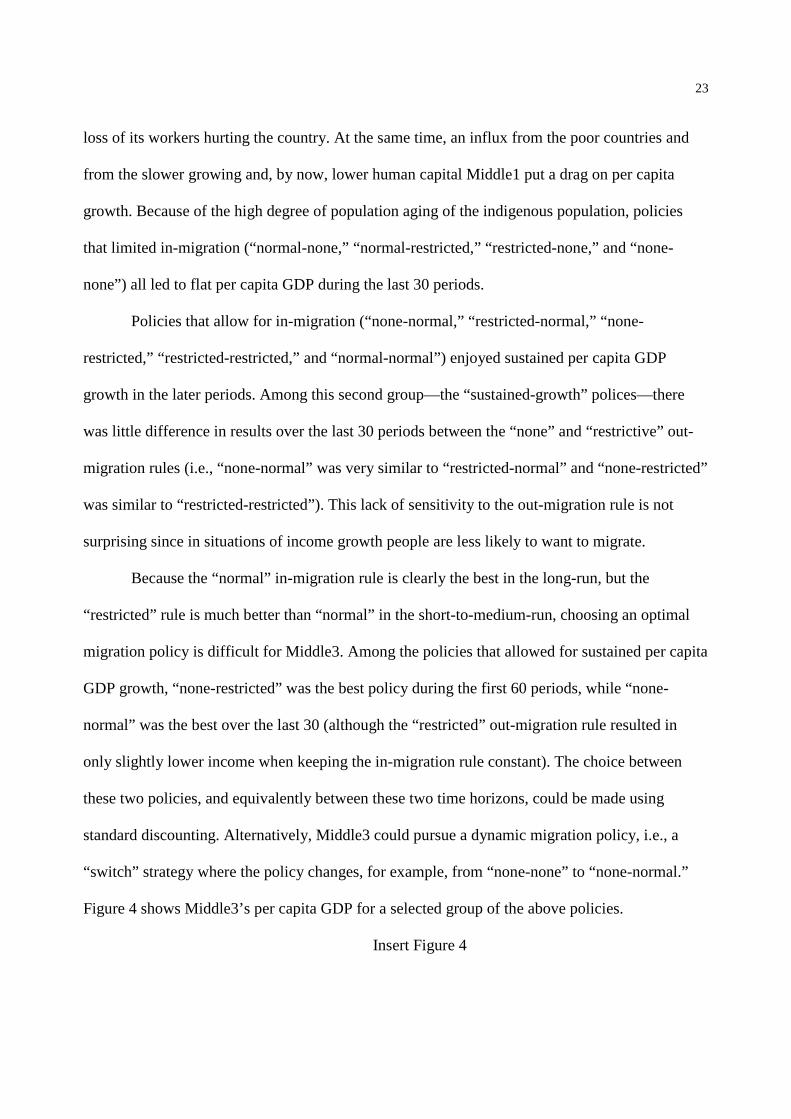
Because the “normal” in-migration rule is clearly the best in the long-run, but the

“restricted” rule is much better than “normal” in the short-to-medium-run, choosing an optimal

migration policy is difficult for Middle3. Among the policies that allowed for sustained per capita

GDP growth, “none-restricted” was the best policy during the first 60 periods, while “none-

normal” was the best over the last 30 (although the “restricted” out-migration rule resulted in

only slightly lower income when keeping the in-migration rule constant). The choice between

these two policies, and equivalently between these two time horizons, could be made using

standard discounting. Alternatively, Middle3 could pursue a dynamic migration policy, i.e., a

“switch” strategy where the policy changes, for example, from “none-none” to “none-normal.”

Figure 4 shows Middle3’s per capita GDP for a selected group of the above policies.

Insert Figure 4

24

6. Population Adjustment Polices: Migration vs. Fertility

In this section we discuss the results of two sets of policy experiments that were aimed at

overcoming the challenges for poor and rich countries, respectively. For the poor countries the

major challenge was affording sufficient investment to achieve growth in the face of rapid

population increases. The rich countries challenge involved affording investment—particularly

spending on environmental quality upgrading—at the time national savings rates were falling

because of the advanced age of their populations. In addition to reporting and analyzing the

results of these two experiments, we place our model in the context of important, new work in the

population-development debate.

6.1 Poor Countries’ Policy Experiment

We assume to reduce their populations the poor countries use the following combinations

of fertility control and out-migration policies:

1. Fertility controla. total fertility rate falls from 5.7 to 2.1 in 25 periods (similar to transition in EastAsia).b. total fertility rate falls from 5.7 to 2.0 in 45 periods (a slower transition rate,closer to Latin America).c. none

2. Migrationa. low level of out-migration (maximum percent of target cohort that may migrateset to 5% for Poor1 and 10% for Poor2).b. normal level of out-migration (maximum percent migrating set to 10% forPoor1 and 15% for Poor2).c. switch policy: maximum percent migrating set to normal level for first 50periods, then switched to low level for remainder of run.

The two population control policies operate at much different rates however, once the

policies have “run their course,” the final total fertility rates are very similar. The two polices

both begin at the 10th period. The “faster” policy (modeled after the East Asian demographic

experience) achieves replacement level fertility in about 25 periods. At this time the policy is

25

switched off, but fertility continues to fall at the same rate as in the other countries that have

completed the demographic transition (the total fertility rate falls to 1.8 by the end of the run). In

the “slower” policy (modeled after the transition experience most similar to that of Latin

American countries) replacement level fertility is achieved around the 55th period, and the total

fertility rate ultimately declines to 1.9. By comparison, the final total fertility rate declines to

around 3.0 for runs with no population control policy.

The migration policy had a significant impact on the size of the total population and

workforce, but a rather negligible impact on per capita GDP or welfare. Different rates of out-

migration can lead to very different population sizes (total and workforce) even when the

different rates exist only for a limited time. Out-migration lowers population in two ways: first,

most obviously, through the loss of the migrants themselves, and second, since we assume the

migrants come from fertile cohorts, migrants cause the number of births to fall (even if fertility

rates do not). Indeed, runs with the same population control policy but different migration

policies (i.e., low vs. switch) finished with significantly different population levels despite having

the same fertility rates and the same migration policy after the 50th period. Furthermore, under the

conditions of these runs, the difference in births is as significant as the difference in number of

migrants in contributing to the difference in population size. The difference in population sizes is

essentially constant after the switch time (period 50). Out-migration over the second half of the

run was influenced more by the relative performance of the various countries than by the out-

migration policy. The runs with the greatest amount of out-migration over the later periods were

the runs with the lowest per capita GDP.

At the levels set in these policies, out-migration primarily influences per capita GDP

through the relationship between aging (or aged dependency) and investment. Out-migration

26

initially raises aged dependency (and thus, lowers investment as a share of GDP), but ultimately

leads to less aging and aged dependency (and, thus, higher investment as a share of GDP). Higher

migration at the end (second half) of the run means higher aged dependency and, thus, lower

investment and GDP over this same time. By contrast, higher migration early in the run means

higher aged dependency early, but lower aged dependency later. Hence, the switch migration

policy tends to mean less aging and, thus, higher GDP at the end of the run.

For the smaller poor country, in some runs that are otherwise similar, a policy of greater

out-migration produces a slightly higher per capita GDP. However, it is abundantly clear, in

comparing runs that differ only in their “population reduction” strategies (migration vs. fertility

decline), lowering fertility is far better than encouraging out-migration for both poor countries.

Population control has an important impact on per capita measures. In the eight runs with

some form of population control, both per capita GDP and welfare were significantly higher than

the four runs with no population control. Fewer births directly improve per capita measures in the

obvious way by lowering the number of mouths, however, lower fertility has more subtle impact

as well. In runs without the austerity policy, population control (or lower fertility rates) led to a

higher share of GDP for investment during much of the run, and to higher investment pools as

well. The higher share of investment occurs more because of higher per capita consumption

(meaning investment is easier to afford) than because of lower youth dependency burdens that

accompany lower fertility. In addition, lower population sizes increase the return to human

capital investment (and, thus, lead to more of this type of investment). Indeed, the runs with

population control all produce substantially higher human capital multipliers. These benefits of

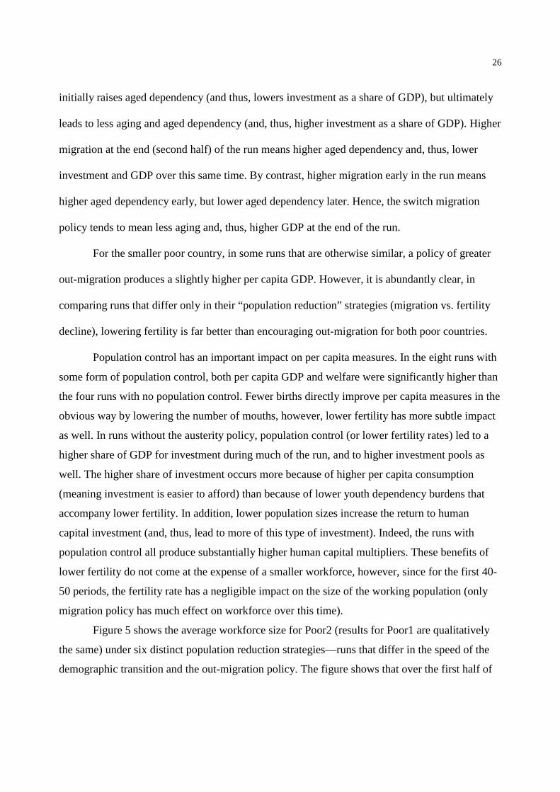
lower fertility do not come at the expense of a smaller workforce, however, since for the first 40-

50 periods, the fertility rate has a negligible impact on the size of the working population (only

migration policy has much effect on workforce over this time).

Figure 5 shows the average workforce size for Poor2 (results for Poor1 are qualitatively

the same) under six distinct population reduction strategies—runs that differ in the speed of the

demographic transition and the out-migration policy. The figure shows that over the first half of

27

the run the out-migration policy is most important; however, over the second half of the run

population varies greatly based on the speed of the fertility transition.

Insert Figure 5

Even though the two population control policies result in similar final total fertility rates

and youth and aged dependency ratios, their different dynamics lead to other important

differences. The faster population control policy produces a smaller population, which enjoys

higher per capita GDP and welfare for much of the run, and a higher share of GDP for investment

(again, primarily because of higher per capita consumption) for the first half of the run. However,

with the faster population control, the countries experience significant and rapid aging over the

second half of the run, and, thus, endure the same challenges aging brings to the rich countries,

i.e., declining investment pools and workforces, and an increasingly higher percentage of

investment going toward environmental quality upgrading. With the slower population control,

aging is not as great a problem. Indeed, under these conditions, workforces decline much less, the

aged dependency ratio increases at a lower rate, the share of GDP for investment is higher for the

second half of the run, as is the investment pool for much of this period, and ultimately, per

capita GDP and welfare are higher. The investment pool still falls, however, under the slower

population control policy, but because of the pool’s larger size, per capita GDP and welfare do

not fall.

The younger and larger populations from the slower population control policy mean the

investment pool peaks much later (approximately 15 periods later) and at a much higher level

(1.6 to 2 times)—even though population is only a third larger—than under the faster population

control policy. This discrepancy is important because the countries spend an increasingly higher

amount of their investment pools on environmental upgrading in the later periods.

28

In runs without population control, both total population and the workforce continue to

increase. Although, youth dependency is higher, the much lower aged dependency means the

share of GDP for investment finishes substantially higher in these runs. Eventually, the

investment pools are larger as well, and, unlike in the population control runs, do not decline.

However, without population control, per capita measures like GDP and welfare do not catch-up

because of the larger population that results when there is no population control, and because of

the greater investment that occurs early on when there is population control.

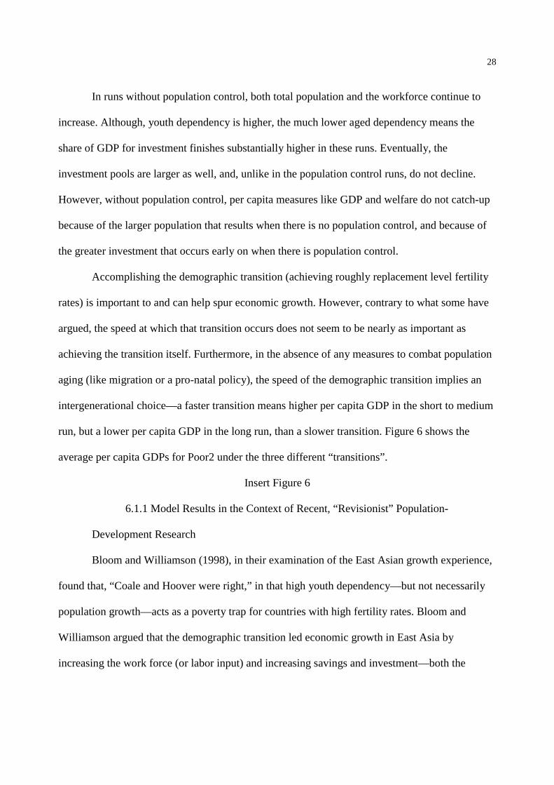
Accomplishing the demographic transition (achieving roughly replacement level fertility

rates) is important to and can help spur economic growth. However, contrary to what some have

argued, the speed at which that transition occurs does not seem to be nearly as important as

achieving the transition itself. Furthermore, in the absence of any measures to combat population

aging (like migration or a pro-natal policy), the speed of the demographic transition implies an

intergenerational choice—a faster transition means higher per capita GDP in the short to medium

run, but a lower per capita GDP in the long run, than a slower transition. Figure 6 shows the

average per capita GDPs for Poor2 under the three different “transitions”.

Insert Figure 6

6.1.1 Model Results in the Context of Recent, “Revisionist” Population-

Development Research

Bloom and Williamson (1998), in their examination of the East Asian growth experience,

found that, “Coale and Hoover were right,” in that high youth dependency—but not necessarily

population growth—acts as a poverty trap for countries with high fertility rates. Bloom and

Williamson argued that the demographic transition led economic growth in East Asia by

increasing the work force (or labor input) and increasing savings and investment—both the

29

supply (by lowering youth dependency) and the demand (through increasing the workforce and

thereby lowering physical capital per worker). According to them, “… population dynamics may

have been the single most important determinant of growth” (Bloom and Williamson, 1998).

In our model, if there is no FDI for the poor countries, but only a population control

policy, the results are very similar to the Coale and Hoover hypothesis as well as Bloom and

Williamson’s findings. The poor countries immediately experience higher per capita GDPs as

well as higher savings rates. The higher savings rates are more a result of this wealth effect—

needing a smaller share of income just for subsistence—than the lowering of youth dependency

burdens since there is some delay before these burdens begin to fall substantially. Mostly, the

fewer number of mouths causes the early increase in per capita GDP as production increases only

slightly. However, the greater amount of investment under the run with lower fertility becomes a

more important part of the higher income as the investments begin to pay-off. Indeed, both poor

countries experience growth in per capita GDP from the beginning of the run, whereas under

similar conditions without any population control (i.e., normal fertility conditions), it takes the

poor countries 30-35 periods before per capita GDP begins to grow. As for investment demands,

the lower student populations do increase the return to human capital investment—an investment

important for long-term economic growth—and the increased production (because of more

physical capital) eventually increases the return to technology investment. In all, these policy

experiments very much confirm the belief that growth of the working-aged population is not at

all bad and may be good for economic growth, but growth of the dependent, non-working

population is likely bad for economic growth.

30

6.2 Rich Countries’ Policy Experiment

As discussed previously, the rich countries’ aging presents challenges for their sustained

growth—both per capita GDP and welfare. Aging means both a declining workforce and, more

importantly, fewer resources going toward investment. One solution for this problem already

discussed is migration—particularly effective when the migrants come from higher fertility

countries. However, a high amount of migration has social and political costs; thus, programs that

may increase indigenous fertility have the attention of policy makers in areas of aging, rich

populations like Europe. Indeed, a recent report of a commission of government, business, and

academic leaders from the OECD countries, published by the Center for Strategic and

International Studies (2002), recommends prompt action to address the problem of aging in

OECD countries. The commission is particularly concerned with the negative impacts on growth

of declining workforces and the crowding effect that pension and health guarantees for the aged

have on public spending in areas like infrastructure and education.

To examine some of the differences between migration and pro-natal, fertility increasing

strategies in addressing the challenges brought on by aging societies, we make a series of runs

with combinations of various increasing fertility regimes with and without migration. In these

runs we do not specify what the pro-natal policy is; rather, we simply assume it is effective to a

particular level. The first pro-natal strategy, “replacement, fast”, causes the total fertility rate

(TFR) to increase from 1.62 in period 10 to 2.19 by period 20. Over the next 25 periods the TFR

falls to 2.09, and remains at this level for the rest of the run. This fertility change is roughly

modeled after the Swedish experience of the 1980s, where the total fertility rate rose from 1.61 in

1983 to 2.13 in 1990 (TFR fell thereafter). (See Andersson 1999 for some explanation of the

Swedish experience.) In the pro-natal policy, “replacement, slow”, it takes 15 years for the TFR

31

to rise to 2. Finally, there is a pro-natal “growth” strategy (run only without migration) that

causes the TFR to increase from 1.62 in period 10 to 2.37 by period 20, before gradually falling

to 2.20 by period 70, after which it remains constant. Furthermore, these three pro-natal policies

can either take effect “early”—beginning, as described above, at period 10—or “late”—

beginning at period 20. The runs with migration use the same migration model previously

described. For comparison purposes, we also run a “base case” that assumes no pro-natal policy

and no migration.

The qualitative aspects of the experiment’s results are the same for both rich countries;

thus, for brevity we concentrate on the results for Rich2. In addition, we separate the

presentation by initially looking at runs without migration and then runs containing migration,

but first we discuss how migration effects population.

Migrants increase the population in two ways: (i) they immediately increase the

population themselves; and (ii) their presence leads to more births (since we assume migrants

come from the most fertile cohorts). Migrants lead to more births both because they increase the

size of the most fertile cohorts and because they often come from countries with higher

indigenous fertility rates. In the terms of demographers, migrants both increase the risk of fertility

and the population at risk. Indeed, a run with migration but no pro-natal policy results in more

births than a run with the most effective pro-natal policy but without migration. Furthermore, this

rise in births from migrants has a much greater impact on the resulting increase in population

than the number of migrants themselves. For example, in the run with migration but no pro-natal

policy, over 100 periods the grand total of migrants was 43, but the final period population was

260 persons larger than in the run without migration or a pro-natal policy. Thus, migration plus

subsequent births can substantially increase the size of a population and reduce its aging without

32

necessarily altering tremendously other more indigenous characteristics (e.g., culture or

ethnicity). Our simplifying migrant assimilation assumptions (e.g., that migrants immediately

induce a change in their new host country’s fertility rates via a weighted average of the migrants’

home country’s rates and the prevailing rates in the destination country’s rates) are clearly that—

simplifications. However, given the previous discussion on the ways migrants affect births, our

assumptions that migrants come from the high fertility cohorts and come to stay—they do not

plan to nor do they ever return to their source country—probably have more to do with migrants’

ultimate impact on a country’s population in our model. In other words, given the lags involved

in human reproduction and the difficulty in government’s changing people’s desired family size,

it is likely the most effective way to increase births is by increasing the population at risk rather

than by increasing the rate of exposure—which of course is precisely what migration does.

For the rich countries, population growth impacts the results in fairly predictable ways. A

larger population means greater production, and hence pollution, and a larger investment pool. A

younger population means a higher percentage of GDP going toward investment. Subtler, per

capita influences on factors like human capital are not present. When the rich countries have

population growth, they are really never investment constrained (even toward the end of the runs

where they are spending heavily on environmental quality upgrading, their investment pools are

large enough to have significant growth enhancing investments as well). Thus, even though the

total populations vary greatly among the runs, the final period human capital multiplier ranges

from only 9.5 to 10.3.

Without migration, the pro-natal policy is important, both in terms of the timing of the

policy’s impact and the effectiveness of its impact. From around the 15th period, only the

“growth” pro-natal policy led to an increase in the size of the workforce (see Figure 7 (a)). In

33

fact, beginning around the mid-point of the run, for the “replacement, slow” policy and

“replacement, fast, late” policy (a policy that does not take effect until the 20th period), the

workforce declined from its initial size. Sometime after the 40th period all runs with a pro-natal

policy had significantly lower aged dependency, and thus, a higher share of GDP for investment,

than in the no migration, no pro-natal case. Significant lag effects are apparent by comparing the

“growth” policy to “growth, late” and comparing “replacement, fast” to “replacement, fast, late”.

Also, most runs had a falling investment share for the last 10 periods. The traces for per capita

GDP and welfare showed similar and predictable patterns: the “growth” policy run was among

the lowest for the first 50 periods, but was clearly the highest for the last 30. The two lagged

policies caught or nearly caught “growth” by the end of the run, but were substantially below it

for most of those last 30 periods.

When migration is added to the various pro-natal policies, all runs experience significant

growth in workforce (see Figure 7 (b)), and there is less difference among the different runs in

general than there was without migration. The run with migration, but without any pro-natal

policy had the smallest population and investment pool, the highest aged dependency, and lowest

investment share, as well as the lowest per capita GDP and welfare for the last 25 periods. There

is particularly little difference between the two sets of lagged runs (“replacement, fast” and

“replacement, fast, late” and “replacement, slow” and “replacement, slow, late”) in per capita

GDP, welfare, investment pool, or pollution. The runs finished with a higher share of GDP going

toward investment than the runs without migration, and with migration this share was steady or

increasing for all at the end of the run. Figures 7 (a) & (b) show the size of the workforce under

the various polices without migration.

Insert Figures 7 (a) & (b)

34

6.2.1 Rich Country Experiment Results in the Context of the Current “Aging

Problem” Debate

In adding migration to a pro-natal strategy, migration seems to function as an insurance

policy by smoothing outcomes, or in other words, making the timing and the success rate of the

pro-natal program less important. In the choice between a migration or pro-natal policy,

migration has the advantage of having a much greater track record of success, as policies to

increase desired fertility in developed countries have been notoriously disappointing—at least for

sustained periods. Furthermore, as long as the goal of the policy is to mitigate the negative effects

of aging, and not for population to reach a constant, replacement level, the amount of migrants

needed is far from overwhelming. The aforementioned commission on aging in OECD countries

recommended making it easier for nonnative residents to achieve citizenship or permanent

residency, and noted the positive impact of high human capital immigrants on the US as well as

the potential synergistic effects of them on their source countries—as is the case for India (Center

for Strategic and International Studies, 2002). In addition, the commission recognized that

policies aimed to increase fertility in developed countries have had mixed results at best.

The UN Population Division, in a recent report (UN, 2000), considered migration as a

solution to the problem of declining and aging populations of developed countries. Ultimately,

the UN, as well as some of the report’s critics (Mayerson, 2001 and Bermingham, 2001), came to

the conclusion that migration is an inadequate means of countering population aging and decline.

The report (and the two critics cited above) rejected the migration option because the large

volume of migrants needed to delay aging in the subject countries would create, “serious social

and political objections” (UN, 2000). In calculating population projections, the UN report

assumed that migrants would immediately experience the average fertility conditions prevailing

35

in their destination country. Yet, both the UN and one of its critics (Mayerson) pointed out the

fact that this is an unrealistic assumption. However, neither the UN nor Mayerson addressed the

logical conclusion that this assumption inflates the number of migrants needed to mitigate aging

in the destination countries, and thus, the social stress caused by the migrants—a primary

objection both expressed to the policy. Another fault of the UN report is assuming that the goal

of such a policy should be “replacement migration” or constant populations, as opposed to simply

mitigating extreme degrees of aging and workforce shrinkage. Likewise, the UN critics (at least

Mayerson and Bermingham) erred in concluding that population growth is necessarily bad—a

conclusion, it appears, driven by a linear interpretation of the IPAT equation, i.e., more

population in developed countries means more pollution.

7. Conclusions

We have tried to develop a model that is “more complete” than most, i.e., a fuller

treatment of population, an economic module that also considers international capital movements,

and some consideration for the environment. But the most important aspects of our work in

differentiating it from others, is our modeling of a diversity of “country types,” and our explicit

modeling of human capital and technology investments/improvements—widely accepted as the

drivers of sustained economic growth. We have allowed countries to differ in initial human

capital and technology levels, and thus, in initial development or wealth levels, as well as in

areas, like age structure, in which there is less likelihood of rapid convergence.

This paper focused on the impacts of different demographic dynamics in our stylized rich,

middle, and poor countries. We found that modeling feedbacks in the population-economy-

environment system means that conclusions derived from the linear IPAT identity do not

necessarily hold. Specifically, migration in the rich countries led to younger, larger populations

36

and ultimately lower levels of environmental impact. In addition, we found that migration into

the rich countries can mitigate the impact of aging (although, perhaps, not reverse it altogether),

and can do so without creating substantial social dislocations since a relatively small number of

migrants may be sufficient. For the middle countries, both source and destination countries of

migrants, the impact of international migrations was much more complex. For at least one middle

country (Middle3), a migration policy needed to be dynamic. Lastly, in the poor countries, as the

population revisionists contend, lowering fertility rates did lead to higher per capita growth; but,

lowering fertility rates was a far more effective way to spur growth than encouraging out-

migration. Yet, the speed at which this transition occurred did not affect the ultimate level or rate

of income growth; rather, it suggested an intergenerational tradeoff. In other words, if age

structure affects savings and investment, and thus economic growth, then a faster demographic

transition (over a slower one) means higher growth in the short to medium run; but because such

a transition results in faster aging as well, it can result in lower income in the longer run.

37

References

Andersson, G. 1999. Childbearing trends in Sweden 1961-1997. European Journal of Population:15 (1), 1-24.

Bermingham, John R. 2001. “Immigration: Not a Solution to Problems of Population Decline andAging,” Population and Environment. Volume 22, Number 4, pp. 355-63.

Bloom, David and David Canning. 2001 “Cumulative Causality, Economic Growth, and theDemographic Transition.” in Population Matters: Demographic Change, Economic Growth, andPoverty in the Developing World. Nancy Birdsall, Allen C. Kelley, and Steven W. Sindingeditors. Oxford: Oxford University Press. Pp. 165-97.

Bloom, David E. and Jeffrey G. Williamson. 1998. “Demographic Transitions and EconomicMiracles in Emerging Asia.” The World Bank Economic Review, 12, 3: 419-455.

Boserup, Ester. 1981. Population and Technological Change: A Study of Long-Term Trends.Chicago: University of Chicago Press.

Center for Strategic and International Studies. 2002. “Meeting the Challenge of Global Aging: AReport to World Leaders from the CSIS Commission on Global Aging.” CSIS: Washington, DC.

Coale, Ansley J. and Edgar Hoover. 1958. Population Growth and Economic Development inLow-Income Countries. Princeton, NJ: Princeton University Press.

Dellink, R.B. 1999. “Environmental-economic modeling: a survey of pollution, abatement andeconomic growth.” Wageningen University, Wageningen, Netherlands.

Ehrlich, Paul R. 1968. The Population Bomb. New York: Ballantine.

Kelley, Allen C. 2001. “The population debate in historical perspective: revisionism revised,” inPopulation Matters: Demographic Change, Economic Growth, and Poverty in the DevelopingWorld. Nancy Birdsall, Allen C. Kelley, and Steven W. Sinding editors. Oxford: OxfordUniversity Press. pp. 24-54.

Kelley, A. C. and Schmidt, R.M.,1994. Population and income change: recent evidence. WorldBank Discussion Paper 249, Washington, DC.

Keyfitz, N. & Flieger, W. (1990). World Population Growth and Aging: Demographic Trends inthe Late Twentieth Century. University of Chicago Press, Chicago.

Lee, Ronald D., Andrew Mason, and Tim Miller. 2001. “Saving, Wealth, and Population,” inPopulation Matters: Demographic Change, Economic Growth, and Poverty in the DevelopingWorld. Nancy Birdsall, Allen C. Kelley, and Steven W. Sinding editors. Oxford: OxfordUniversity Press. Pp. 137-64

38

Loschel, Andreas. 2002. “Technological Change in Economic Models of Environmental Policy:A Survey.” Working paper, University of Mannheim, Germany.

Mason, A. (1987). National Saving Rates and Population Growth: A New Model and NewEvidence. In Johnson, D. G. & Lee, R. D. (Eds.), Population Growth and EconomicDevelopment: Issues and Evidence, University of Wisconsin Press, Madison (pp. 523-560).

Mason, A. (1988). Saving, Economic Growth and Demographic Change. Population andDevelopment Review, 14 (March), 113-144.

Meyerson, Frederick A.B. 2001. “Replacement Migration: A Questionable Tactic for Delayingthe Inevitable Effects of Fertility Transition,” Population and Environment. Volume 22, Number4, pp. 401-9.

OECD. (1995). The OECD Input-Output Database. Organization for Economic Co-operation andDevelopment, Paris.

Sanderson, Warren C. 1980. Economic-Demographic Simulation Models: A Review of TheirUsefulness for Policy Analysis. RR-80-14. IIASA. Laxenburg, Austria.

Sanderson, W.C. 1992. Simulation models of economic, demographic, and environmentalinteractions: are they on a sustainable development path? Working paper WP-92-87, IIASA,Laxenburg, Austria.

Schmidt, S. R. and Launsby, R.G. (1992). Understanding Industrial Designed Experiments,Third Edition. Air Academy Press, Colorado Springs.

Simon, J. L. (1977). The Economics of Population Growth. Princeton University Press,Princeton, NJ.

Simon, Julian. 1981. The Ultimate Resource. Princeton, NJ: Princeton University Press.

United Nations Population Division. 2000. Replacement Migration: Is it a Solution to Decliningand Ageing Populations? New York: United Nations.

Williamson, Jeffrey G. and Higgins, Matthew. 2001. “The Accumulation and DemographyConnection in East Asia.” in Population Change and Economic Development in East Asia. Editedby Andrew Mason, Stanford, CA: Stanford University Press, pp. 123-54.

World Bank, 1994. World Tables 1994. The World Bank, Washington, DC.

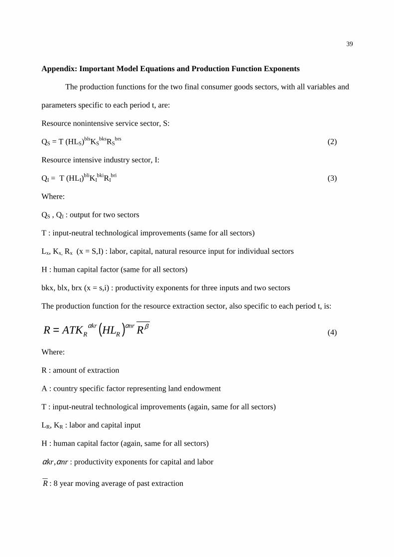
39

Appendix: Important Model Equations and Production Function Exponents

The production functions for the two final consumer goods sectors, with all variables and

parameters specific to each period t, are:

Resource nonintensive service sector, S:

QS = T (HLS)blsKSbksRS

brs (2)

Resource intensive industry sector, I:

QI = T (HLI)bliKI

bkiRIbri (3)

Where:

QS , QI : output for two sectors

T : input-neutral technological improvements (same for all sectors)

Lx, Kx, Rx (x = S,I) : labor, capital, natural resource input for individual sectors

H : human capital factor (same for all sectors)

bkx, blx, brx (x = s,i) : productivity exponents for three inputs and two sectors

The production function for the resource extraction sector, also specific to each period t, is:

( ) βαα RHLATKR nrR

krR= (4)

Where:

R : amount of extraction

A : country specific factor representing land endowment

T : input-neutral technological improvements (again, same for all sectors)

LR, KR : labor and capital input

H : human capital factor (again, same for all sectors)

nrkr αα , : productivity exponents for capital and labor

R : 8 year moving average of past extraction

40

ß : country specific drag parameter based on the extent of recent extraction (less than -1).

The exponents used in Equations 2-4 were estimated from empirical data of factor shares

using The OECD Input-Output Database (1995), as applied to the stylized definitions of our

aggregate sectors.

Place Table A-1 here

Environmental Quality Module Equations, again with all variables and parameters

specific to each period t, are:

PEQEQ −= 0 (5)

( )Π−= 1PP (6)

φθ CEQW = (7)

φθ +=1 (8)

GDPdgk −=θ (9)

( )ef−=Π 199.0 (10)

where EQ is environmental quality, EQ0 is environmental quality in a pure state

(arbitrarily set high enough so EQ is positive), P is effective pollution consumed, P is pollution

produced, Π is the percentage remediated, W is welfare, C is per capita final goods consumption,

GDP is per capita GDP, and k, d, and g are positives constants (all less than 1.0 and k > dg) that

set bounds for the welfare weight on environmental quality. The percentage remediated is based

on the amount of investment in environmental quality upgrading per unit of pollution produced,

e, and the ease of remediation, f (currently set to 0.05). Thus, the maximum amount remediated

is 99 percent of pollution produced.

41

Table 1: Initial Country EndowmentsTechnologymultiplier1

Humancapital

multiplier2

Landendowment3

Totalpopulation

TFR Ageddependency

ratio

Youthdependency

ratioRich1 3.0 3.0 2.5 182 1.81 0.244 0.536

Rich2 3.0 3.0 10.0 300 1.81 0.244 0.536

Middle1 2.0 2.0 5.0 204 3.58 0.073 1.086

Middle2 2.0 2.0 10.0 200 2.47 0.105 0.741

Middle3 2.0 2.0 15.0 300 1.88 0.106 0.635

Poor1 1.2 1.0 20.0 465 5.96 0.071 1.392

Poor2 1.2 1.0 20.0 200 5.96 0.071 1.392

Notes: (1) The T in Equations 2-4. (2) The H in Equations 2-4. (3) The A in Equation 4.

Table A-1: Production Function ExponentsExtraction/resource

replenishmentResourceintensive“industry”

Resourcenonintensive

“service”Labor share 0.3 0.45 0.6Capital share 0.7 0.20 0.3Natural resource share 0.35 0.1

42

Figure 1: Welfare levels for all countries in the base case run.

Figure 2: Per capita GDP for all countries when the base case is run without the environmentalmodule (thus, no environmental drag), without population dynamics (thus, no population drag),without FDI, and without the ability to increase technology or human capital via investment (i.e.,constant technology and human capital levels).

0

50

100

150

200

250

300

350

400

450

0 20 40 60 80

rich1

rich2

middle1

middle2

middle3

poor1

poor2

0

5

10

15

20

25

0 20 40 60 80

rich1

rich2

middle1

middle2

middle3

poor1

poor2

43

Figure 3. The right-hand axis shows, for the larger rich country, the savings rate with and withoutmigration. With migration there was less aging in the rich country; thus, the savings rate did notfall as much—indeed it leveled—over the second half of the run. The left-hand axis showswelfare for the same country. Welfare diverges because the higher savings rate with migrationtranslated into a larger investment pool and more spending on environmental quality upgradingand, thus, higher welfare levels.

0

50

100

150

200

250

300

350

400

0

0.05

0.1

0.15

0.2

0.25

welfare, migration welfare, no migration

savings rate no migration savings rate migration

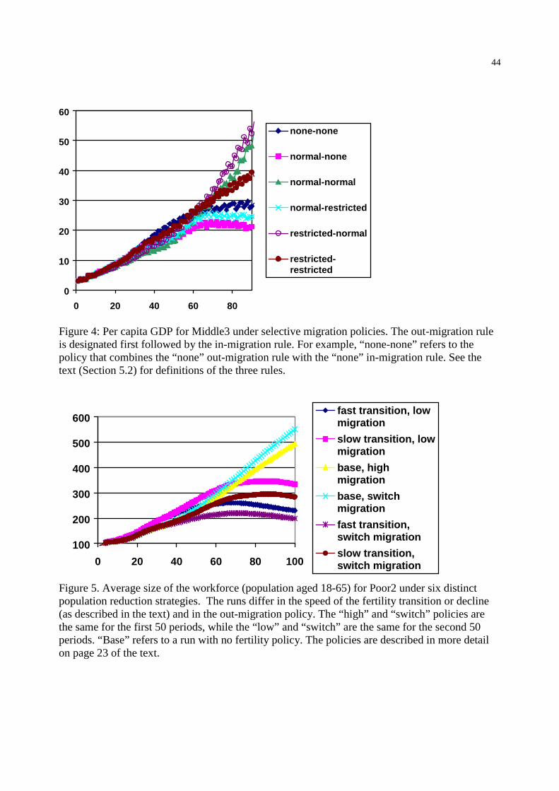
44

Figure 4: Per capita GDP for Middle3 under selective migration policies. The out-migration ruleis designated first followed by the in-migration rule. For example, “none-none” refers to thepolicy that combines the “none” out-migration rule with the “none” in-migration rule. See thetext (Section 5.2) for definitions of the three rules.

Figure 5. Average size of the workforce (population aged 18-65) for Poor2 under six distinctpopulation reduction strategies. The runs differ in the speed of the fertility transition or decline(as described in the text) and in the out-migration policy. The “high” and “switch” policies arethe same for the first 50 periods, while the “low” and “switch” are the same for the second 50periods. “Base” refers to a run with no fertility policy. The policies are described in more detailon page 23 of the text.

0

10

20

30

40

50

60

0 20 40 60 80

none-none

normal-none

normal-normal

normal-restricted

restricted-normal

restricted-restricted

100

200

300

400

500

600

0 20 40 60 80 100

fast transition, lowmigration

slow transition, lowmigration

base, highmigration

base, switchmigration

fast transition,switch migration

slow transition,switch migration

45

Figure 6. Average per capita GDP for Poor2 under three different fertility transitions: “base”refers to fertility control (c) as described on page 23 in the text; “fast transition” to fertilitycontrol (a); and “slow transition” to fertility control (b). Results are qualitatively the same forPoor1.

Figure 7 (a) The size of workforce for Rich2 under pro-natal polices that do not includemigration. The changes in fertility that correspond to the three policies, “replacement, fast,”“replacement, slow,” and “growth” are defined in the text. The distinction “late” means the policytakes effect in period 20 rather than period 10. The default or base case of no policy is “no pro-natal.”

0

5

10

15

20

25

30

35

0 50 100

base

fast transition

slow transition

100

120

140

160

180

200

220

240

0 20 40 60 80 100

replmnt, fast

replcmnt, slow

growth

replacement, fast-late

growth, late

no pro-natal

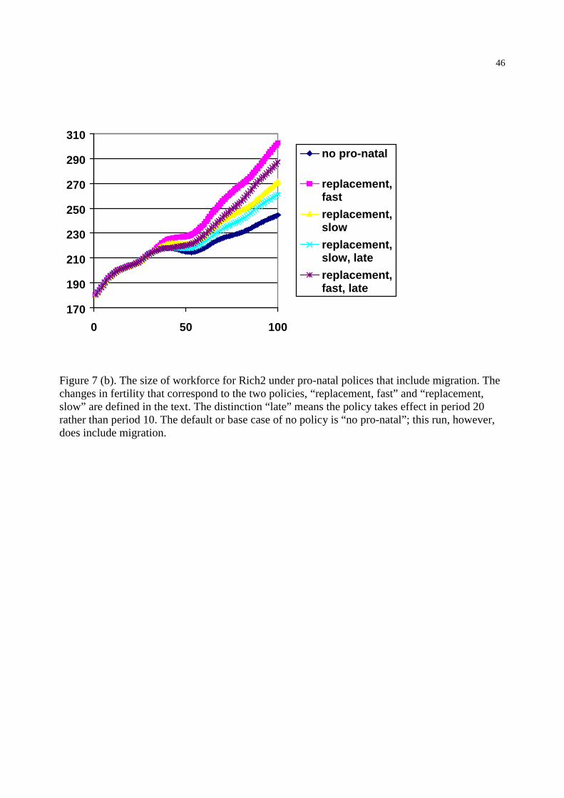
46

Figure 7 (b). The size of workforce for Rich2 under pro-natal polices that include migration. Thechanges in fertility that correspond to the two policies, “replacement, fast” and “replacement,slow” are defined in the text. The distinction “late” means the policy takes effect in period 20rather than period 10. The default or base case of no policy is “no pro-natal”; this run, however,does include migration.

170

190

210

230

250

270

290

310

0 50 100

no pro-natal

replacement,fast

replacement,slow

replacement,slow, late

replacement,fast, late