Delivery: an open–source model–based

Bayesian seismic inversion program ⋆

James Gunning a,∗, Michael E. Glinsky b

aCSIRO Division of Petroleum Resources, Ian Wark Laboratory, Bayview Ave.,

Clayton, Victoria, 3168, Australia, ph. +61 3 9545 8396, fax +61 3 9545 8380

bBHP Billiton Petroleum, 1360 Post Oak Boulevard Suite 150, Houston, Texas

77056, USA

Abstract

We introduce a new open–source toolkit for model–based Bayesian seismic inver-sion called Delivery. The prior model in Delivery is a trace–local layer stack,with rock physics information taken from log analysis and layer times initialisedfrom picks. We allow for uncertainty in both the fluid type and saturation in reser-voir layers: variation in seismic responses due to fluid effects are taken into accountvia Gassman’s equation. Multiple stacks are supported, so the software implicitlyperforms a full AVO inversion using approximate Zoeppritz equations. The likeli-hood function is formed from a convolutional model with specified wavelet(s) andnoise level(s). Uncertainties and irresolvabilities in the inverted models are capturedby the generation of multiple stochastic models from the Bayesian posterior (usingMarkov Chain Monte Carlo methods), all of which acceptably match the seismicdata, log data, and rough initial picks of the horizons. Post-inversion analysis ofthe inverted stochastic models then facilitates the answering of commercially use-ful questions, e.g. the probability of hydrocarbons, the expected reservoir volumeand its uncertainty, and the distribution of net sand. Delivery is written in java,and thus platform independent, but the SU data backbone makes the inversionparticularly suited to Unix/Linux environments and cluster systems.

Key words: seismic, inversion, AVO, Bayesian, stochastic, geostatistics, MarkovChain Monte Carlo, open–source,

⋆ Updated manuscript with additional Appendices from citation (Gunning and Glin-sky, 2004). Please cite as both (Gunning and Glinsky, 2004) and the website.∗ Corresponding author.

Email address: James.Gunning@csiro.au (James Gunning).

Article originally published in Computers & Geosciences 30 (2004)

Contents

1 Introduction 3

2 Outline of the model 6

2.1 Description and notation of the local layer model 8

2.2 Construction of the prior 10

3 The forward model 14

3.1 Computing the synthetic seismic 14

3.2 Isopach constraints 18

4 Sampling from the posterior 19

4.1 Mode location and local covariance 20

4.2 Mode enumeration 22

4.3 Sampling 23

5 The software 27

6 Examples 28

6.1 Sand Wedge 28

6.2 Net–to–gross wedge 28

6.3 Simple single–trace fluid detection problem 31

6.4 Field Example 31

7 Conclusions 32

Appendix 1: Typical computation of effective rock properties 36

Appendix 2: Error sampling rates 37

Appendix 3: Mode–location starting points 37

Appendix 4: An Independence Sampler 39

Appendix 5: Modified SU trace formats for properties 40

5.1 Model–prior trace formats 40

2

5.2 Stochastic trace outputs 40

Appendix 6: Wavelet format 41

Appendix 7: Usage of the code 41

7.1 Inputs 41

7.2 Outputs 43

Appendix 8: Incorporation of Floating Grain models into Delivery 44

8.1 Floating grain effects 44

8.2 Recommended methodology 46

8.3 Conversion to Delivery formats 46

8.4 Rock trends 47

8.5 Model system 48

8.6 Inversion Analysis of Posteriors 49

8.7 Delivery Implementation details 51

8.8 Inputs/Outputs 54

Appendix 9: Vertical model–stacking functionality 54

Appendix 10: Internal fluid–contact modelling 58

10.1 Upscaling rules 60

10.2 New outputs in the realisations SU file 60

10.3 Example Inversion 61

10.4 Likely Issues 63

Appendix 11: Model selection facilities 64

1 Introduction

The basic purpose of the seismic experiment in the oil exploration business hasalways been the extraction of information regarding the location, size and na-ture of hydrocarbon reserves in the subsurface. To say this is to also grant that

3

the analysis of seismic data is necessarily and always an inversion problem:we do not measure reservoir locations and sizes; we measure reflected wave-forms at the surface, from which information about potential reservoir zonesis extracted by a sequence of processing steps (stacking, migration etc) thatare fundamentally inversion calculations designed to put reflection responsesat their correct positions in time and space.

Such inversion calculations invariably depend on assumptions about the char-acter of the geological heterogeneity that are usually described informally(“gentle dips”, “weak impedance contrasts” etc), but could equally well becouched in formal probabilistic language. Further, such assumptions often holdwell across a range of geological environments, and are of a nature that leadsto generic processing formulae (e.g. Kirchoff migration) that may be appliedby the practitioner with merely formal assent to the assumptions underlyingtheir validity. From this point of view, we can say that traditional inversionis fundamentally based on a model of the subsurface, but no particular detailsof that model appear explicitly in the resulting formulae. These inversions canalso be claimed to have integrated certain portions of our geological knowledge,in that the empowering assumptions have been made plausible by observationand experience of typical geological structures.

By this line of argument, traditional inversion can be seen as an attempt toexplain the observed surface data by appeal to a broad (but definite) model ofthe subsurface, which yields congenial formulae when we incorporate certaingeological or rock-physics facts (“weak reflections” etc). It is then no great stepof faith to assert that inversion techniques ought to incorporate more definiteforms of knowledge about the subsurface structure, such as explicit surfaces orbodies comprised of certain known rock types whose loading behaviour maybe well characterised.

Such a step is in fact no longer contentious: it has long been agreed in the geo-physical community that seismic inversion tools ought to use whatever rock–physics knowledge is regionally available in order to constrain the considerablenon–uniqueness encountered in traditional inversion methodologies. Further,in an exploration or early–appraisal context, some limited log or core data areusually available, from which additional constraints on likely fluid types, timeand depth horizons etc can be constructed.

In practice, such knowledge is difficult to incorporate into “model–free” meth-ods like sparse–spike inversion, even though these methods have a sound geo-physical basis. Conversely, detailed multi–property models of the reservoir –such as geostatistical earth models – are often weak in their connection togeophysical principles: the relationship to seismic data is often embodied inarbitrary regression or neural–network mappings that implicitly hope that thecorrect rock physics has been divined in the calibration process.

4

Another long–settled consensus is that the inversion process is incurably non–unique: the question of interest is no longer “what is such and such a quantity”,but “what is the multi–component distribution of the quantities of interest”(fluids, pay zone rock volume etc) and the implications of this distribution fordevelopment decisions. The development of this distribution by the integrationof information from disparate sources and disciplines with the seismic data isnow the central problem of seismic inversion. An interesting aspect of this con-sensus is that most workers in seismic inversion (and closely related problemslike reservoir history matching) now concede that the most satisfactory way toapproach the non–uniqueness and data–integration problems is via a Bayesianformalism 1 . These approaches use explicit models for the quantities of inter-est: typically a suite of layers or facies, whose location and internal propertiesare the properties we wish to invert for. Examples of such work are Omre andTjelmeland (1997), Eide et al. (2002), Buland and Omre (2000), Buland et al.(2003), Eidsvik et al. (2002), Leguijt (2001) and Gunning (2000) in the con-text of seismic problems, and the many papers of Oliver and his school in thecontext of reservoir dynamics problems, e.g. Chu et al. (1995), Oliver (1997),Oliver (1996). Newer kinds of Bayesian inversion are also appearing, wherethe model uncertainty itself (e.g. the number of layers) is taken into account,e.g. Malinverno (2002). It is recognised also that the posterior distribution ofinterest is usually quite complicated and impossible to extract analytically; itsimpact on decisions will have to be made from Monte Carlo type studies basedon samples drawn from the posterior.

Nevertheless, the use of model–based Bayesian techniques in seismic inversionat this point in time is still novel or unusual, for a mixture of reasons. Themain reason is undoubtedly the lack of accessible software for performing suchinversions, and the associated lack of fine control of such systems even whenthey are available as commercial products. Bayesian inversion methodologiesare unlikely to ever become “black–box” routines which practitioners can applyblindly, and successful inversions will usually be the result of some iterativeprocess involving some adjustment of the model–prior parameters and choiceof algorithms. Such flexibility is hard to achieve in “black–box” algorithms.A second reason is that the amount of effort required to construct a suitableprior model of the rock physics and geological surfaces of interest will alwaysbe non–trivial, though repeated experience of such an exercise will reduce therequired effort with time. This effort is justified by the fact that a Bayesianinversion constructed around an appropriate prior will always produce morereliable predictions than an inversion technique which does not integrate theregional rock physics or geological knowledge. This fact will be obvious if wedo the thought experiment of asking what happens when the seismic data

1 other approaches to stabilising the inverse problem via regularisation or parameterelimination are perhaps best seen as varieties of Bayesian priors, perhaps augmentedwith parsimony–inducing devices like the Bayes information criterion.

5

has poor signal to noise ratio. We assert that the use of Bayesian model–based inversion techniques should become far more widespread once the firstmentioned obstacle above is overcome.

We do not presume in this paper to offer even a partial critique of non–modelbased inversion techniques from a Bayesian point of view: the reader will beable to do this for themselves after consideration of the methods and principlesoutlined below. The aim of this paper is rather to introduce a new open–sourcesoftware tool Delivery for Bayesian seismic inversion, and demonstrate howthis code implements a model–based Bayesian approach to the inversion prob-lem. The software described in this paper is a trace–based inversion routine,and is designed to draw stochastic samples from the posterior distribution ofa set of reservoir parameters that are salient for both reservoir volumetricsand geophysical modelling. The exposition will cover the choice of the modelparameters, construction of the prior model, the development of the forwardseismic model and the associated likelihood functions, discuss the mappingof the posterior density, and sketch the methods used for sampling stochasticrealisations from the posterior density. The latter involves use of sophisticatedMarkov Chain Monte Carlo (MCMC) techniques for multiple models that arerelatively new in the petroleum industry.

The main content of the paper is laid out as follows; in section 2 the overallframework and design of the inversion problem is outlined. Section 2.1 describesthe basic model and suitable notation, section 2.2 outlines the construction ofthe prior model, and section 3 describes the forward model and associatedlikelihood. Section 4 covers the problems of mode mapping and sampling fromthe posterior. An outline of the software is provided in section 5: it is releasedunder a generic open–source licence rather like the popular GNU and open–BSD style licenses. A discussion of a suite of example/test cases is given insection 6, and conclusions are offered in section 7.

2 Outline of the model

The inversion routine described in this paper is a trace–based algorithm, de-signed to operate in a computing environment where a local seismic trace(usually post-stack, post-migration) in Seismic Unix (SU) format (Cohen andStockwell, 1998) is piped to the routine in conjunction with a set of parametersdescribing the local prior model, also in SU format. Stochastic realisations arethen drawn from the posterior and written out, also in SU format. The detailsof these formats are discussed in section 5. Inverting on a trace-by–trace ba-sis amounts to an assumption that the traces are independent, and this canbe guaranteed by decimating the seismic data to a transverse sampling scaleequal to the longest transverse correlation appropriate for the local geology.

6

Spacings of a few hundred metres may be appropriate. Working with indepen-dent traces has the great advantage that the inversion calculation is massivelyparallelizable, and the computation may be farmed out by scatter–gather op-erations on cluster systems. Finer scale models may then be reconstructed byinterpolation if desired.

Inversion calculations on systems with inter–trace correlations are very dif-ficult to sample from rigorously. Sketches of a suitable theory are containedin Eide (1997), Eide et al. (2002), Abrahamsen et al. (1997), Huage et al.(1998) and Gunning (2000), from which we offer the following potted sum-mary. If the variables to be inverted are jointly multivariate Gaussian, someanalytical work can be done which yields a sequential trace–based algorithm,but the matrix sizes required to account for correlations from adjacent tracesare very large. Models which use non–Gaussian models for distributing facies(e.g. the indicator model used in Gunning (2000)) require methods that involvemultiple inversions over the whole field in order to develop certain necessarymarginal distributions. These calculations are very demanding, even for purelymulti–Gaussian models.

From another point of view, the sheer difficulty of rigorously sampling frominter–trace correlated inversion problems is the price of modelling at a scalefiner than the transverse correlation length of the sediments (and/or surfaces)of interest, which is commonly several hundred metres or more. We know fromthe Nyquist theorem that any random signal can be largely reconstructed bysampling at the Nyquist rate corresponding to this correlation length, andintermediate values can be recovered by smooth interpolation. This is a strongargument for performing inversion studies at a coarser scale than the fine scale(say 10-30m) associated with the acquisition geometry 2

By assuming the inter–trace correlation is negligible, the inversion can proceedon an independent trace basis, and the incorporation of non–linear effects likefluid substitution, and discrete components of the parameter space (what typeof fluid, presence or absence of a layer etc) become computationally feasible.In short, the correct sampling from systems with inter–trace correlations isprobably only possible in systems with fully multi–Gaussian distributions ofproperties, but such a restriction is too great when we wish to study systemswith strong nonlinear effect like fluid substitution and discrete components likelayer pinchouts or uncertain fluids. The latter, more interesting problems onlybecome possible if we reduce the transverse sampling rate.

2 The choise of the transverse sampling rate depends also on the form of the trans-verse correlation dependence, since, e.g. smooth surfaces are better reconstructedby interpolation than noisy ones. This requires some judgement. Possible correla-tion lengths appropriate to various geological environments are discussed in Deutsch(2002).

7

The model used in this inversion is somewhat coarser than that commonlyused in geocellular models. At each trace location, the time–region of interestis regarded as a stack of layers, typically a metre to several tens of metresin size. Each layer is generically a mixture of two “end-member” rock types:a permeable reservoir member, and an impermeable non–reservoir member.the balance of these two is determined by a layer net–to–gross (NG), and theinternal structure of mixed layers (0 < NG < 1) is assumed to be finely hori-zontally laminated, so acoustic properties can be computed using an effectivemedium theory appropriate for this assumption. Seismic energy reflects at theboundaries between layers, producing a surface signal that may be syntheti-cally computed, given an incident wavelet and all the requisite rock properties.

2.1 Description and notation of the local layer model

At the current trace location, the set of rock layers in the inversion region isfundamentally modelled in time rather than depth. The depth d enters as arelatively weakly controlling parameter of the rock properties, but time is afundamental variable in terms of computing seismic responses, so is the betterchoice of variable for the basic parameterisation.

Models in depth are more fundamentally useful for reservoir decision making,but we adopt a flow wherein depth models can be created from any timemodel by a simple post–processing step. Depth constraints can take the formof thickness constraints or absolute depth constraints, and both of these can beapplied either through the prior parameters or the isopach criterion we discusslater. Either way, the generation of depth models will require the specificationof a reference layer, from which all layer depths will be hung or supportedas required. This scheme ensures that depth and time models are mutuallyconsistent.

The model consists of Nl layers, with ti the top of layer i. Layer i is boundedby the times (ti, ti+1), i = 1...Nl. An additional parameter, tbase, is required tospecified the bottom of the model. Figure 1 shows a cartoon of the model.

Each layer is modelled as a mixture of two finely–laminated end–member rocktypes; a permeable member like sand or carbonate, and an impermeable mem-ber, such as shale or mudstone. The subscript f is used generically to denotethese facies, but also s for the permeable member (think “sand”) and m for theimpermeable (“mud”). The net-to-gross NG specifies the ratio of permeable toimpermeable rock by volume. Pure shales or other impermeable rocks can bemodelled by NG = 0. Hydrocarbons may be present only in the permeablemembers of the laminated mixture.

The properties of permeable rocks that we explicitly model are the p–wave

8

tt

Reflection coefficients Synthetic seismic

waveletm = {ttop, NG, f R, vp,R, vs,R, r NR, vp,NR, vs,NR, r b,vp,b,r h,vp,h,Sh}

Model parameters per layer:

R = reservoir rocks

NR = impermeable rocks

b = brine

h = hydrocarbon

Full suite of model parameters:

M = {m1,m2,m3,...}

shale

shale

shale

oil-filled laminated sand

brine-filled laminated sand

brine-filled laminated sand

Fig. 1. Schematic of the local layer–based model and its notation. For descriptionof the model parameters see the main text. The reflection coefficient sequence andsynthetic seismic are part of the forward model of section 3.

velocity vp,s, the shear velocity vs,s, and porosity φs, but for impermeablemembers we use vp,m, vs,m, and density ρm. Facies are assumed isotropic. Theserock properties are in general controlled by a loading curve which dependsprimarily on depth but also possibly a low–frequency interval velocity (LFIV)(derived perhaps from the migration), as explained in section 2.2.3.

Permeable members that are susceptible of fluid substitution will also requireknowledge of the dry matrix grain properties, and saturations, densities and p–wave velocities of the fluids undergoing substitution. For a particular rock type,the grain properties are taken as known, but the fluid saturations, densitiesand velocities can form part of the stochastic model.

The set of parameters describing the full acoustic properties for layer i, boundedby times ti−1, ti, with hydrocarbon h present, is then

m = {d, LFIV, NG, φs, vp,s, vs,s, ρm, vp,m, vs,m, ρb, vp,b, ρh, vp,h, Sh}, f = s,m,

(1)

at each trace. A i subscript is implicit for all quantities. If the layer is a pureimpermeable rock (NG = 0), this simplifies to

m = {d, LFIV, ρm, vp,m, vs,m}. (2)

The union of these parameters with the layer times ti (and the final bottom-layer base time tbase) then forms the full model vector of interest. Since thetimes are the dominant variables, it is convenient to arrange them to occurfirst in the full model vector, so this is assembled as

m = {t1, t2, . . . , tNl, tNl,base,mlayer–1,mlayer–2, . . .mlayer–Nl

, A,B}. (3)

The extra stochastic factors A,B affect the synthetic seismic and are explainedin section 3.1.4. Hereon we use dm for the dimensionality of the model m.

9

An additional feature is that some parameters may be common to severallayers (e.g. in many cases the LFIV is an average across many layers), so theunderlying model vector will map all duplicate instances to the one variable(so, e.g. there may be only one LFIV in the overall model vector).

Also, it is sometimes useful to “synchronise” the rock–matrix properties be-tween two layers, so that if they have the same end–members, acoustic con-trasts at the interface must be entirely due to fluid effects. In this case theunderlying parametrisation will map all rock-matrix affecting parameters inthe lower layer to those of the layer above, and remove all redundancies in themodel vector.

2.2 Construction of the prior

2.2.1 Layer times

Before inversion, the times ti are not known precisely, but are modelled asstochastic variables with prior distributions N(ti, σ

2ti). The mean and standard

deviation are estimated from horizon picking and approximate uncertainty es-timates (e.g. a half–loop or so may be chosen for the σti). The prior distributionon layer times is supplemented by an ordering criterion which says that layerscannot swap:

ti ≥ ti−1, (4)

so the prior for the layer times is actually a product of truncated Gaussianswith delta functions at the endpoints absorbing the mis–ordered configurations.A typical scenario is that the top and bottom of a large packet of layers havebeen picked reasonably accurately, but the time–location of the intermediatesurfaces is not well known.

The truncation rules allow the useful possibility of pinchouts. For example,layer 2 may disappear if we have t3 = t2, in which case the interface at thistime comprises a contrast between layer 1 properties and layer 3 properties,providing t3 > t1. Modelling pinchouts in this way then requires a specificalgorithm for determining where the pinchouts occur from a given set of (un-truncated) layer times ti. We have used this scheme:

(1) Form a sort order based on the layer prior time distributions uncertain-ties σti (sorting in increasing order), and from the top layer down as asecondary sort order if some σti ’s are identical.

(2) From the set of candidate time samples {ti} (which will not in generalsatisfy (4)), proceed to fix the times in the sort order above, truncating

10

values to preserve the ordering criterion (4) as we proceed. For example,if the sort order is {1,4,2,3}, and we have a set t1 < t4 < t3 < t2, this willend up truncated at t1, (t2 = t4), (t3 = t4), t4.

This recipe is designed to allow the “better picked” horizons higher priority insetting the layer boundary sequence.

Sometimes it is desirable to force a layer to permanently pinchout in someregion of space, and thus effectively drop out of the model: see Appendix 5.1for a discussion.

2.2.2 Prior beliefs about hydrocarbons

The modeller will have formed beliefs about the probability of certain kindsof hydrocarbons in each layer, informed by non-seismic sources such as pres-sure data or resistivity logs. A relative prior probability is assigned to eachhydrocarbon type in each layer on this basis. Specifically, each layer i maybear fluids; oil (o), gas (g), brine (b), or low–saturation gas (l). The modellermust specify the prior probabilities of each of these phases, on a layer basis,as Fio, Fig, Fib, Fil respectively, with Fio + Fig + Fib + Fil = 1.

Depending on the likely hydraulic communication between layers, the hydro-carbons allowed to be present in the permeable layers may be subjected to adensity–ordering criterion, e.g. oil is not permitted above gas in two adjacentpermeable layers. At least three types of density ordering rule can be envisaged:

(1) None. Any fluids are allowed in any permeable layer.(2) Partial. Fluids are density ordered for all adjacent permeable layers not

separated by an impermeable layer.(3) Full. Fluids are density ordered across the entire reservoir model, regard-

less of whether there are impermeable layers separating permeable ones.

The default density ordering is {b, l, o, g}, with low–saturation gas placedbetween brine and oil because it usually arises as a residual saturation trailbehind migrating hydrocarbons.

The set of possible fluids in each layer (as implied by the prior probabilities)are combined with a rule for density ordering to then enumerate a discrete setof possible fluid combinations k = 1 . . . NF . 3 Suppose the fluid–combinationk corresponds to the set of fluid labels fik ∈ {b, l, g, o}, i = 1 . . . Nl. Then the

3 E.g. a two layer system under ordering rule (3), where it is known that gas (andlow sat. gas) cannot occur (Fig = Fil = 0), may have the allowable set {(brine,brine) : (oil, brine) : (oil, oil)}, so NF = 3.

11

prior probability of this fluid–combination is taken to be

pk =

∏

i Fi,fik∑NF

k′=1

∏

i Fi,fik′

. (5)

Note that in multi–layer systems, this makes the marginal prior probability ofobtaining a certain fluid in a given layer quite different to the prior probabilityspecified on a layer basis, simply because of the ordering criterion 4 . In sub-sequent discussions, the prior probability of each distinct fluid combination kenumerated in this way is denoted pk.

Supplementing this fluid categorisation, it is desirable also to model the fluidsaturations Sif , f = o, g, b, l for each fluid type. The two phases present aretaken as brine (b) & hydrocarbon (o,g,l). The petrophysicist can assign Gaus-sian stochastic priors Sif ∼ N(Sif , σSif

), truncated 5 outside [0, 1] to thesesaturation parameters, based on regional knowledge.

2.2.3 Prior information about rock properties

Net–to–gross

The net–to–gross prior distribution is taken as N(NG, σ2NG

), truncated within[0, 1]. The mean and standard deviation of this distribution can be determinedby consultation with the geologist. A broad prior may be used to reflect un-certain knowledge.

Trend curves

From logging information in wells drilled through intervals deemed to be repre-sentative of the rock behaviour in the region to be inverted, a set of regressionrelationships for useful acoustic properties in all the facies is developed. Thepoints used in these local “trend curves” are computed using a known referencefluid (typically, a brine) in place of the in–situ fluid, and the basic acoustic

4 For example, in the two–layer problem of the preceeding footnote, if the priorprobability of oil in each layer had been specified as, say, 0.6, the 3 combina-tions would have probabilities proportional to 0.42, 0.6 × 0.4, 0.62 respectively, or0.21, 0.316, 0.474 after normalisation, so the post–ordering prior probability of oil inlayer 2 is 0.474, and in layer 1 is 0.316 + 0.474 = 0.79.5 The algorithms in this code treat truncated Gaussian distributions as a mixtureof a true truncated Gaussian plus delta functions at the trunction points, of weightequal to the truncated probability. This has the advantage of giving non–vanishingprobability to certain physically reasonable scenarios, like NG = 0, or a layer pin-chout.

12

properties (ρ, vp, vs) of these reference fluids have to be established (the refer-ence fluid may vary with facies for various reasons). These “reference–fluid”properties may also be slightly uncertain, with Normal distributions modellingtheir variation about a mean.

The trend curves are a set of rock-matrix velocities (p–wave, s–wave) vpf ,vsf , and density ρf (or porosity φf ) regressions for all end-member rocks. Forreservoir–members, the porosity is used in preference to the density 6 , and theset of regressions is

φf = (Aφ + Bφvpf ) ± σφf

vsf = (Avs+ Bvs

vpf ) ± σsf (7)

vpf = (Avp+ Bvp

d + CvpLFIV) ± σpf ,

where d=depth. The last equation models vp as linear in d = depth (com-paction etc) and linear in the low–frequency interval velocity (LFIV); a lo-cal mean vertical p-wave velocity obtained from pure seismic data like VSP,moveout or stacking considerations. Such a regression can capture most strati-graphic, compaction and overpressure effects.

For impermeable rocks, the porosity is of no direct interest, and the densityis regressed directly on vpf using a Gardner–Gardner–Gregory (GGG) typerelationship:

log ρf = (log Aρ + Bρ log vpf ) ± σρf or: ρf = AρvBρ

pf ± σρf

vsf = (Avs+ Bvs

vpf ) ± σsf (8)

vpf = (Avp+ Bvp

× depth + Cvp× LFIV) ± σpf .

Typically, Bρ ≈ 0.25. Since the range of densities and velocities in a singlerock type is not large, this GGG type regression can also be cast as a linearregression over a suitable range.

The regression errors (σpf ,σsf , . . . ) used in these relationships are the predic-tion errors formed from linear regression studies, which yield t–distributionsfor the predictive distribution. We approximate this result by taking the priorto be of Normal form, with variance set to the regression variance. For exam-ple, the prior for vp,f is N(Avp

+ Bvpd + Cvp

LFIV, σ2pf ). This approximation is

exact in the limit of large data.

6 Density is computed from

ρsat = (1 − φ)ρg + φρfluid (6)

for permeable members.

13

2.2.4 Fluid properties

We have also, from measurements or prior information, Gaussian prior distri-butions for the fluid p–wave velocities N(vp, σvp

) and densities N(ρ, σρ) (fromwhich the bulk moduli distribution can be computed) for the reference brinesand any possible hydrocarbons.

3 The forward model

The Bayesian paradigm requires a likelihood function which specifies how prob-able the data are, given a particular model. This requires calculation of a syn-thetic seismic trace from the suite of layers and their properties, and formingthe likelihood by comparing the seismic data and the synthetic seismic. Theforward seismic model is a simple convolutional model, which treats layers asisotropic homogeneous entities with effective properties computed from thesuccessive application of Gassman fluid substitution in the permeable rocksand Backus averaging with the impermeable rocks.

There may be additional constraints in the form of isopach specifications, wherea particular layer–thickness is known to within some error by direct observa-tion, or other source of knowledge. The isopach constraint, being independentfrom the seismic, forms its own likelihood, and the product of the syntheticseismic likelihood and the isopach likelihood form the overall likelihood for theproblem.

3.1 Computing the synthetic seismic

3.1.1 Rock mixtures

When two different isotropic rocks are mixed at a fine (sub–seismic resolution)scale with strong horizontal layering, it is well known that the effective acousticproperties of the mixture can be computed using the Backus average (Mavkoet al. (1998), p. 92). This assumes that the wavelengths are long comparedto the fine–scale laminations represented by the net–to–gross measure. Thestandard formulae are

1

Meff

=NG

Mpermeable

+1 − NG

Mimpermeable

, (9)

14

where M can stand for either the p-wave (M) or shear (µ) modulus (µeff =ρeffv

2s,eff, Meff = Keff + 4

3µeff = ρeffv

2p,eff), and the effective density is

ρeff = NGρpermeable + (1 − NG)ρimpermeable. (10)

3.1.2 Fluid substitution in permeable rocks

When the saturation of a particular hydrocarbon is not trivially 0 or 1, wetake the hydrocarbon and brine phases to be well mixed on the finest scale, sothe fluid can be treated as an effective fluid (see p. 205, Mavko et al. (1998))whose properties are computed using the Reuss average

K−1fluid =

Six

Kix

+1 − Six

Kib

. (11)

When the effective fluid replaces brine in the pore space, the saturated rock haseffective elastic parameters that are computed from the usual low-frequencyGassman rules (Mavko et al., 1998): viz

Ksat

Kg − Ksat

=Kdry

Kg − Kdry

+Kfluid

φs(Kg − Kfluid). (12)

The Mpermeable in the Backus relation (9) will be the p–wave modulus for perme-able rock after fluid substution via Gassman (only the permeable end–memberwill undergo fluid substitution). Here Kdry is the dry rock bulk modulus, Kg isthe bulk modulus of rock mineral grains, Kfluid the bulk modulus of the substi-tuted fluid (gas/oil/brine/low-sat. gas), and Ksat the effective bulk modulus ofthe saturated rock. The shear modulus µ is unchanged by fluid substitution.

Under replacement of the reference fluid b by a fluid fl (a two–phase mix ofbrine and hydrocarbon h), the Gassman law can be written 7

Ksat,fl

Kg − Ksat,fl

− Ksat,b

Kg − Ksat,b

=Kfl

φs(Kg − Kfl)− Kb

φs(Kg − Kb). (13)

3.1.3 Typical computation sequence

A typical computation sequence for computing the set of effective properties fora laminated, fluid–substituted rock layer would run as described in Appendix 1.Prior to computing the synthetic seismic, the effective properties of all thelayers must be computed following this recipe.

7 Assuming no pressure effects on the dry modulus Kdry.

15

3.1.4 The synthetic seismic and seismic–likelihood

Given a wavelet w, an observed seismic S, and an estimate of the seismic noisepower σ2

s , we can use the reflectivities R associated with effective–propertycontrasts between layers to construct the synthetic seismic appropriate to anyparticular stack. The synthetic is taken to be

Ssyn ≡ w ∗ R, (14)

where we use an FFT for the convolution, and w and R will be discretised atthe same sampling rate ∆t as the seismic data set S for the trace. The set ofdelta functions in R are projected onto the discretised time–grid using a 4–point Lagrange interpolation scheme (Abramowitz and Stegun, 1965) based onthe nearest 4 samples to the time of a spike. This ensures the synthetic seismichas smooth derivatives with respect to the layer times, a crucial property inthe minimisation routines that are described in section 4.1.

Available data traces S may be near or far-offset (or both), and an appropriatewavelet w will be provided for each. The P–P reflection coefficient for smalllayer constrasts and incident angles θ is 8

Rpp =1

2

(

∆ρ

ρ+

∆vp

vp

)

+ θ2

∆vp

2 vp

−2 vs

2(

∆ρρ

+ 2 ∆vs

vs

)

vp2

, (15)

with

ρ = (ρ1 + ρ2)/2 (16)

vp = (vp,1 + vp,2)/2 (17)

vs = (vs,1 + vs,2)/2 (18)

∆ρ = ρ2 − ρ1 (19)

∆vp = vp,2 − vp,1 (20)

∆vs = vs,2 − vs,1 (21)

and layer 2 below layer 1. All properties in these formulae are effective prop-erties obtained as per Appendix 1. The coefficient of θ2 is usually called theAVO gradient.

Due to anisotropy and other effects related to background AVO rota-tion (Castagna and Backus, 1993), some corrections to this expression may

8 From the small–contrast Zoeppritz equation for Rpp(θ), expanded to O(θ2) (topof p.63, Mavko (1998))

16

be required, so the reflection coefficient will take the form

Rpp(A,B) =A

2

(

∆ρ

ρ+

∆vp

vp

)

+ Bθ2

∆vp

2 vp

−2 vs

2(

∆ρρ

+ 2 ∆vs

vs

)

vp2

, (22)

where the factors A and B may be stochastic, typically Gaussian with meansclose to unity and small variances: A ∼ N(A, σA), B ∼ N(B, σB).

Explicitly, θ2 for a given stack is obtained from the Dix equation. The stackhas average stack velocity Vst, event–time Tst and mean–square stack offset

〈X2st〉 =

(X3st,max − X3

st,min)

3(Xst,max − Xst,min), (23)

from which the θ2 at a given interface is computed as

θ2 =v2

p,1

V 4stT

2st/〈X2

st〉. (24)

The likelihood function associated with the synthetic seismic mismatch is con-structed as

Lseis = exp(−ferror

∑

error–sampling points

(Ssyn − S)2/2σ2s)), (25)

where the range of the error–sampling points is computed from the prior mean–layer time range and the wavelet characteristics as per figure 2. Within thisrange, the points used in the error sum are spaced at the maximum multipleof the seismic sampling time p∆t which is smaller than the optimal errorsampling time ∆Ts derived in Appendix 2 (i.e. p∆t ≤ ∆Ts). The correctionfactor ferror ≡ p∆t/∆Ts, is designed to recovery the error that would obtain ifthe error trace were discretised at exactly ∆Ts. The signal–to–noise ratio SN

is implied by the noise level σs supplied by the user, with typically SN ≈ 3.

If both normal–incidence (small θ) and far–offset seismic data are available(“large” θ), we model the overall likelihood as a product of likelihoods fornormal–incidence and far–offset angles.

The stack information required by the likelihood model thus comprises the pa-rameters Vst (stack velocity to event), Xst,max (far offset), Xst,min (near offset),and Tst (event time), a wavelet appropriate for the stack, and the noise levelσs.

17

Tabove

Tbelow

Ran

ge o

f err

or -

sam

plin

g po

ints

mod

el in

terv

al (

<t 1

> to

<t b

ase>

from

prio

r)

<t2>=top reflector (prior)

Region above model in which assumption of no reflectors is implied

Region below model in which assumption of no reflectors is implied

wavelet coda

wavelet precursor

t=0

t=0

<tNl>=bottom reflector (prior)

Error trace

Fig. 2. Diagram indicating range over which the error samples are computed. Ingeneral Tabove,below are free parameters, but we take Tabove = wavelet–coda andTbelow = wavelet–precursor as a sensible choice, since this allows the full reflectionenergy from the top and bottom reflections to enter the error count for models nottoo different to the mean prior model. The error is usually acquired by a sum overa subsampled range (circled samples), the sub–sampling rate computed as per themain text.

3.2 Isopach constraints

For certain layers there may be a constraint on the thickness which is obtainedfrom well data, or kriged maps of layer thicknesses constrained to well data.Let j = 1, . . . Nt label the layers on which such a constraint is imposed. Thethickness of the layer must match a known thickness ∆Zj, within an error σ∆Zj

18

specified. This can be represented in a likelihood function

Liso = exp(−∑

j

(vj,p,eff(tj − tj−1) − ∆Zj)2

2σ2∆Zj

) (26)

Similarly, constraints on the net–to–gross may be imposed by kriging net–to–gross estimates from well data. These will then be used to populate theprior–model traces with a spatially–variable net–to–gross.

4 Sampling from the posterior

The posterior distribution for the inversion problem is a simultaneous modelselection and model sampling problem. The selection problem is primarilythat of choosing a model from the suite of models associated with the fluidcombinations described in section 2.2.2. For a particular combination k offluids in the permeable layers, the model vector mk can be constructed fromthe union of all relevent parameters in equation (3). Hydrocarbon terms areomitted if the layer contains brine. Any fixed or irrelevant parameters arediscarded. Different possible fluid combination will then yield model vectorsmk of different dimension.

A further model–selection problem can also emerge from strong multimodalitythat may appear in the posterior for any particular fluid combination. If, for afixed fluid combination, the posterior contains strongly isolated modes, sam-pling from this density is best approached by regarding the modes as separatemodels and incorporating them into the model–selection problem.

Model–selection problems can proceed in two ways. The first is to seek themarginal probability of the kth model P (k|d) by integrating out all the conti-nous variables mk in the problem and then drawing samples via the decomposi-tion P (k,mk|d) = P (mk|k, d)P (k|d). The problem is to find reliable estimatesof P (k|d) when the necessary integrals cannot be done analytically. Methodsto form such estimates using MCMC methods are described in Raftery (1996),and tend to focus on harmonic means of the likelihood computed with MCMCsamples drawn from the conditional P (mk|k, d). Preliminary experiments haveshown some difficulty in stabilising the various estimators described by Raftery.The best estimator we have found is the full Laplace estimator, based on theposterior covariance matrix obtained by Newton updates at the mode. Thisforms the basis of an “independence sampler”, whose implementation detailsare described in Appendix 4.

The second method samples for the full posterior P (k,mk|d) by constructinga hybrid MCMC scheme that make jumps between the various models as well

19

as jumps within the continuous parameter space of each model. Such methodsare variously described as model jumping methods, e.g. Andrieu et al. (2001),Phillips and Smith (1996); we implement the methods described by Adrieu.

For a fixed fluid combination k (of prior probability pk), the posterior distribu-tion of the model parameters mk should clearly be proportional to the productof the prior distributions with all the applicable likelihoods:

Π(mk|S) ∼ Lseis(m′

k|S)Liso(m′

k)P (mk), (27)

where the full prior is

P (mk) =pk

(2π)dmk/2|Ck|1/2

exp(−1

2(mk − mk)

T C−1k (mk − mk)) (28)

Note that the likelihood functions are evaluated for the model m′

k obtainedfrom mk after applying time ordering (section 2.2.1) and truncation of anyvalues to their appropriate physical range of validity (e.g. 0 ≤ NG ≤ 1). In agreat majority of cases in realistic models, m′

k = mk. The prior mean vectormk and inverse covariance C−1

k can be built directly from the description ofthe prior in section 2.2.

Efficient sampling from the posterior will require location of all the feasiblemodes for a particular fluid combination, plus an estimate of the dispersion ateach mode. The latter is usually taken as the local covariance associated witha Gaussian approximation to the local density.

4.1 Mode location and local covariance

Location of the modes is usually performed by searching for minima of thenegative log–posterior starting from strategic points. For each fluid combina-tion, the full model vector m can easily have dimension of d = O(50) or more,so this minimisation is quite demanding. The log–posterior surface is smoothfor all parameters except where a layer pinches out, since the disappearinglayer causes an abrupt discontuity in the reflection coefficient. Such problemscan be tackled with variable metric methods like BFGS minimizers 9 speciallyadapted to detect solutions that lie along the lines of dicontinuity (typically atsome ti+1 = ti). Still, very best-case d–dimension minimisation usually requiresO(d2) function evaluations, with the coefficient being in the order of 10-100.

9 The code actually uses an adaptation of Verrill’s java UNCMIN routines (Koontzand Weiss, 1982), which implement both BFGS and Hessian–based Newton methods.

20

Observe also that the function evaluation is a synthetic seismic (over Nt sam-ples), plus prior, plus isopach, so the work count for this is O(d2 +Nt log(Nt)),which is typically O(103) flops.

This accounting shows that the overall minimisation, performed over all d pa-rameters will be quite slow. In practice, some of the parameters affect theposterior much more strongly than others. Layer times, p–velocities and den-sities have strong effects, whereas, e.g. hydrocarbon saturations have ratherweak ones. This observation leads to a scheme wherein the minimisation iscarried out over a subset of important parameters (say 2 or three per layer),and the remainder are estimated after the minimisation terminates using asequence of Newton iterates as follows.

4.1.1 Newton updates

If the prior distribution for mk is multi–Gaussian, with negative log–likelihood− log(P (mk)) ∼ (mk−m)C−1

m (mk−m), and the likelihood function is of form

log(L(m|D)) ∼ −1

2(f(mk) − y)T .diag(σ−2

i ).(f(mk) − y), (29)

then the posterior mode m can be estimated by linearising f(m) about aninitial guess m0 using the standard inverse theory result (Tarantola, 1987)

X =∇f(m0) (30)

Cm = (XT C−1D X + C−1

m )−1 (31)

m= Cm(XT C−1D (y + Xm0 − f(m0)) + C−1

m m) (32)

where CD = diag(σ2i ). Here the f(m) will be read from the seismic (25) or

isopach likelihoods (26).

The updates encountered in the code are all cases where the error covarianceis diagonal, so the formulae are more simply stated in terms of the scaledresiduals e:

e(m0) = C−1/2D (f(m0) − y) (33)

X ≡∇e(m0) (34)

d= Xm0 − e(m0) (35)

Cm = (XT X + C−1m )−1 (36)

m= Cm(XTd + C−1m m) (37)

21

The gradient X is evaluated by finite differences, and the scheme can be it-erated by replacing m0 ← m at the end. It converges quadratically to thetrue mode if the path crosses no layer-pinchouts. Typically, after minimisationusing, say, BFGS methods over the dominant parameters in m, only a few New-ton iterates are required to get decent estimates of the remaining parameters,and the posterior covariance matrix Cm comes along for free.

4.2 Mode enumeration

Incorporation of the isopach likelihood alone will likely yield an approximatelyquadratic log–posterior function, which has a single mode. This mode mayalso be quite tight, especially at the wells. Conversely, the synthetic seismiclikelihood is likely to be strongly multimodal, especially in the time parameters.

For this reason, we always perform a small set of Newton updates (say 5) tothe prior based on the isopach likelihood before commencing a minimisationstep for the entire posterior. The “partial–posterior” formed from the productof the prior and isopach constraint will be approximately multi–Gaussian, andthe mode and covariance of this distribution are then used to choose startingpoints for a set of subsequent minimisation calls. The subset of parametersused in the modified BFGS minimisation routines are typically the layer timesti, the impermeable layer p–velocities vp and the net–to–gross NG. Other com-binations are conceivable and perhaps better. The initial starting values of thenon–time parameters are taken from the “partial–posterior” mean, and a setof starting times are assembled as per the description in Appendix 3. A runof subspace minimisations looping over this set of starting configurations willyield a set of points hopefully in the vicinity of global modes. Duplicates areeliminated. Figure 3 indicates how the sequence of dispersed starting points,subspace minimisation, and global Newton methods converge to the desiredseparate modes.

The remaining candidate points then undergo a set of Newton updates (about10) for the full model. Subsequently, any modes that look wildly implausibleare eliminated 10 . If a mode is acceptable, the Newton-updated mean andcovariance are stored, along with a measure of the mode weight such as thelikelihood at the peak of the mode, and the Laplace–estimator weight, equa-tion (59), described in Appendix 4. Diagnostic routines capable of drawinggraphs of the log posterior centered at the mode are useful in checking thecharacter of the mode and the adequacy of the Gaussian approximation.

In cases where the seismic likelihood value obtained after these local optimi-

10 the remaining freedom in the frozen parameters is unlikely to redeem a bad loop–skip

22

t

subspace minima

full-space local minima

Newton steps

Newton steps

vs

start

start

Fig. 3. Minimisation scheme consisting of subspace minimisations (the subspacerepresented by t) starting from dispersed points, followed by global Newton steps,yielding a set of local minima in the full parameter space.

sations looks poor (or for other reasons), a global optimisation step may beinitiated operating on the subvector of layer times, with non-time propertiesfixed at their prior+isopach means. The initiation conditions for this step aredesigned to detect trapping of the BFGS/Newton optimisers in poor local so-lutions. The globally optimal t values are then used as starting points for theNewton optimiser. The global optimiser uses the Differential Evolution geneticalgorithm of Storn and Price (1997).

4.3 Sampling

The overall Markov Chain for the sampling is generated by a kernel that flipsrapidly between two kinds of proposals: (a) jumps to different models, and (b)jumps within the current model. Currently the scheme chooses one of thesemoves with a 50% probability at each step, and performs a within–model jumpor model–jump according to the schemes described below. This is the mixturehybrid–kernel of section 2.3 in Brooks (1998). Special “moves” for unusualsituations can also be devised, and are generally safe to use providing they aredrawn independently of the current state of the chain.

23

Within–model jumps

For single–model d–dimensional problems that have smooth densities, a Metro-polis–Hastings sampler that is both efficient and robust is the scaled reversible–jump random–walk sampler (RWM) described in Ch. 11 of Gelman et al.(1995). In this sampler, the jumps are drawn from the distribution q(mnew|mold) =N(mold, s

2C), where C is the estimated covariance at the mode, and s is a scalefactor set to s = 2.4/

√d. For multi–Gaussian distributions, this scale factor

leads to optimal sampling efficiency for this class of samplers (acceptance ratesnear 0.23), and the sampling efficiency is then about 0.3/d. The proposals mnew

drawn from q(mnew|mold) are then time–ordered and truncated if necessary (asper section 4) to produce m′

new and then used to compute the full posteriordensity

Π(mnew|S) = Lseis(m′

new|S)Liso(m′

new)P (mnew). (38)

If the posterior were perfectly multi–Gaussian, samples could be drawn froman independence sampler (Brooks, 1998) using a Gaussian proposal density,which would be 100% efficient since successive samples are independent, butthe assumption of a compact Gaussian distribution for the proposal densityin a Metropolis technique will force undersampling of regions of the posteriorthat may have thick tails. Such regions appear reasonably likely when crosssections of the log–posterior are plotted as diagnostic output: significant non–parabolicity is usually evident in the time–parameters (see figure 4).

Hence, for random walks within a fixed model, we use the RWM sampler wherethe covariance used is that produced by the sequence on Newton updates atthe mode. The initial state is taken at the mode peak. Jumps that produce anunphysical state are treated as having zero likelihood. The acceptance proba-bility for a jump mold → mnew is the usual rule

α = min(1,Π(mnew|S)

Π(mold|S). (39)

Note that the actual proposal probability q does not need to be evaluated, butthe appropriate scaling for it is crucial.

Model jumping

Jumps between models have to be made with care so as to preserve reversibility.A notable feature of the set of models to be sampled from is that a great manyparameters are common to all models (times, rock parameters etc), and onlythe fluid characteristics distinguish the models corresponding to different fluid

24

vs_s

3200 3400 3600 3800 4000 4200 4

5

6

7

8

9

vs_m

3200 3400 3600 3800 4000 4200 4

5

6

7

8

9

vp_s

8400 8600 8800 9000 9200 9400 4

5

6

7

8

9

vp_m

8600 8800 9000 9200 9400 9600 9800 4

5

6

7

8

9

t

4.30 4.35 4.40 4.45 4.50 4.55 4.60 4.65 4

5

6

7

8

9

rho_m

2.30 2.32 2.34 2.36 2.38 2.40 2.42 4

5

6

7

8

9

phi_s

0.26 0.28 0.30 0.32 0.34 0.36 4

5

6

7

8

9

NG

0.2 0.4 0.6 0.8 1.0 1.2 4

5

6

7

8

9

Fig. 4. Series of log–posterior cross–sections taken through the maximum–likelihoodpoint found from the optimisation step and the sequence of Newton updates. Cross—sections are shown for the parameters shown, in all relevant layers, over a range of 2standard deviations as computed from the local covariance matrix. Near–Gaussianparameters will show symmetric parabolas with a rise of +2 at the endpoints, butnon–Gaussianity is evidenced by skewed or a-symmetric profiles, most obvious inthe case of the time parameters in this instance.

states. For example, if a jump involves introducing gas into a layer, the modelvector is augmented by the gas velocity, saturation, and density (if they are notfixed). The models are thus good examples of the nested structures discussedin Andrieu et al. (2001), and the algorithms below are simple instances of themethods discussed in section 3 of that paper.

25

Suppose the models m1 and m2 are partitioned into components as m1 ={m∗

12,m′

12}, m2 = {m∗

21,m′

21}, the asterisk denoting common elements andthe prime non–common parameters (so m∗

12 = m∗

21 is the same set). We haveestimates of the maximum likelihood model values m1 = {m∗

12,m′

12} andm2 = {m∗

21,m′

21} from the sequence of minimisation steps for each mode,and it is invariably the case that the shared parameters will have differentvalues at each of these maximum–likelihood points. A jump from model 1 to2 is then performed by the mapping

m2,new = {m∗

12,old + (m∗

21 − m∗

12),m′

21} (40)

where m′

21 is drawn from a suitable proposal distribution q12(m′

21), which weusually take to be the prior for those components, since the fluid parametersare uncorrelated with the rest of the model in the prior:

q12(m′

21) =∏

new fluid components parameters j in modelpj(m

′

21,j) (41)

A reverse jump, from 2 to 1, would have invoked the proposal probabilityq21(m

′

12) for the components of model 1 not present in model 2. The jumpfrom model 1 to 2 is then accepted with probability

α = min(1,π(m21)q21(m

′

12)

π(m12)q12(m′

21)). (42)

where π(·) is the full posterior density of equation (27), including the dimension–varying terms in the prior.

In the thought–experiment limit that the likelihood functions are trivially unity(we “switch” them off) this jumping scheme will result in certain acceptance,as the qij(·) densities will cancel exactly with corresponding terms in the prior.The likelihoods are expected to be moderately weak functions of the fluid prop-erties, so this seems a reasonable choice. Further, in many practical scenarios,the fluid constants may be sufficiently well known that they are fixed for theinversion, in which case the models share all the parameters, and the q termsdisappear from equation (42).

The linear translation embodied in equation (40) is based on an plausible as-sumption that the ’shape’ of the posterior density for the common parametersremains roughly the same across all the models, but the position may vary.Corrections to this assumption can be attempted by rescaling the mappingusing scale–factors estimated from covariance estimates – which introduces aconstant Jacobian term into equation (42) – but numerical experiments havenot shown that this embellishment significantly improves the acceptance rates.

26

Mixing has generally been found to be very good when jumps are performedbetween various fluid states using this scheme. When multimodality in theposterior due to loop–skipping occurs, mixing can be more problematic, andthe posterior samples should be checked carefully to ensure mixing is adequate.Various options for detecting and auto–correcting for this problem, using dec-imation estimates computed from the time–series in the Markov chain (Ch. 7,Gelman et al. (1995)), have been added to the code.

5 The software

The Delivery inversion software is written in java, a design decision ratherunusual in the context of numerically intensive scientific software. It shouldrun on java implementations from 1.2 on. The advent of hotspot and just–in–time (JIT) compiler technology has made java a very much more efficientlanguage than in its early days as a purely interpreted language (see the JavaNumerics website as an entry point 11 . The core cpu demands in the code are(a) linear algebra calls, for which we use the efficient CERN colt library 12

and (b) FFTs, for which we provide a library operating on primitive double[]or colt DenseDoubleMatrix1D arrays, and the former have been demonstratedto be as fast as C on the platforms we use.

On platforms with modern hotspot or JIT compilers, the code is estimatedto run somewhere within a factor of 2-5 of the speed of a C++ implementa-tion, and has the advantage of being platform independent, free of memory–management bugs, and has been simpler to develop using the large suite oflibraries now standard in java 1.2 and its successors.

In practice, the inversion code will likely be run in an operating system thatallows piping of input and output data in the form of SU streams, and theattractive possibility of clustering the calculation means that it will likely berun on some flavour of unix or Linux.

Some explanation of the files required for input/output and usage is given inAppendix 7. The inversion is chiefly driven by an XML file that specifies thenecessary rock–physics, layer descriptions, and information about the seismic.A quality schema–driven GUI editor expressly developed for the constructionof this XML file is also available at the website: further details are in theAppendix.

11 Boisvert, R., Pozo, R., 2003. The Java Numerics website, http://math.nist.gov/javanumerics/.12 Hoschek, W., 2003. The CERN colt java library, http://dsd.lbl.gov/~hoschek/colt.

27

The code is available for download (Gunning, 2003), under a generic open–source agreement. Improvements to the code are welcome to be submitted tothe author. A set of simple examples is available in the distribution.

6 Examples

6.1 Sand Wedge

A simple but useful test problem is one where a wedge of sand is pinched out bysurrounding shale layers. This is modelled as a three layer problem, where weexpect the inversion to force pinching–out in the region where no sand exists,if the signal–to–noise ratio is favourable and the sand–shale acoustic contrastis adequate.

In this example, the prior time parameters are independent of the trace, sothere is no information in the prior to help detect the wedge shape. The inter-nal layer times have considerable prior uncertainty (20ms, 50ms respectively).Figure 5 illustrates pre and post inversion stochastic samples of the layers,displayed with many realisations per trace. Here the noise strength is about1/4 of the peak reflection response when the wedge is thick (i.e. away fromtuning effects).

This test problem shows how the inverter can readily unscramble tuning effectsfrom rock–physics to produce an unbiased inversion of a layer pinchout.

6.2 Net–to–gross wedge

Another useful test problem is where a slab of shaly sand is gradually madecleaner from left to right across a seismic section, and embedded in the mixingshale. As the net–to–gross increases, the reflection strength improves, and theposterior distribution of the net–to–gross and layer thickness is of interest.

In this example, the only parameters that varies areally is the mean net–to–gross: this is fixed to be the same as the “truth–case” model, but has a (verybroad) prior standard deviation of σNG = 0.3. Figure 6 illustrates pre and postinversion estimates of the net–to–gross distribution parameters, superposed onthe truth case. This example is also used to demonstrate the convergence of theMCMC sampler, for which we show some characteristic plots of the randomwalk for the inversion on trace 8. Here the prior was loosened considerably toNG ∼ N(0.45, 0.72). The chains are always started at the maximum likelihoodpoint, so ’burn–in’ times are generally very short.

28

1.7

1.8

1.9

2.0

2.1

1.7

1.8

1.9

2.0

2.1

(a) (b) (c)

(d) (e) (f)

1.80

1.85

1.90

1.95

2.00

2.05

1.80

1.85

1.90

1.95

2.00

2.05

2.10

0

20

40

60

80

100

1.88

1.90

1.92

1.94

1.96

1.98

2.00

Thi

ckne

ss (

m)

laye

r-tim

es

Fig. 5. (a) Truth case wedge model, (b) truth case seismic, (d) pre-inversion stochas-tic samples (i.e. drawn from prior distribution only, (e) post inversion samples(100 per trace), (c) p10, p50, p90 quantiles for the layer times of the wedge, and (f)p10, p50, p90 quantiles of the wedge thickness. Note how the wedge layer time un-certainty increases to the prior when the wedge pinches out, as there is no longera significant reflection event to facilitate the detection of this horizon: the inverterdoes not care where the horizon is, as long as it pinches out. The wedge thickness(zero) is still well constrained though.

This test problem shows that the inverter produces a relatively unbiased inver-sion for the net–to–gross, but subject to increasing uncertainty as the reflectinglayer dims out.

29

1.80

1.85

1.90

1.95

2.00

0.0

0.2

0.4

0.6

0.8

1.0

0.0

0.2

0.4

0.6

0.8

1.0

(b)

(a)

(c)

(d) (e)

(f) (g)

p10p10

p90

p90

p50p50

time

(sec

s)

Net

-to-

gros

s

Net-to-gross

Nea

r re

flect

ion

coef

ficie

nt

Nea

r re

flect

ion

coef

ficie

ntN

et-t

o-gr

oss

Net

-to-

gros

s

-0.1

0.0

0.1

0.2

0.3

0.4

0.5

0.6

0.0

0.2

0.4

0.6

0.8

1.0

PRIOR POSTERIOR

POSTERIOR

POSTERIORPOSTERIOR

POSTERIOR

10000

5

10

15

20

25

30

2000 4000 6000 8000 10

4

Iteration

trace number

trace number trace number

trace numbertrace number

Log(

likel

ihoo

d)

0.0 0.2 0.4 0.6 0.80.08

0.10

0.12

0.14

0.16

0.18

0.20

Fig. 6. (a) Truth case seismic for net–to–gross (NG) wedge model, (b) pre–inversion(prior) spread of NG as show by p10, p50, p90 quantiles; truth–case shown dashed, (c)as per (b), but post–inversion. Inset (d) shows the near–stack reflection coefficientvariations, and (e) the associated samples of NG. The signal–to–noise ratio hereis very favourable, with noise 1/10th of the peak seismic response. The residualuncertainty in the NG is due to the fact that there is also uncertainty in the layervelocity variations. The seismic constrains primarily the reflection coefficient, but thesystem indeterminacy will still allow appreciable variation in the NG. Convergence& mixing of the MCMC scheme is illustrated for a highly non–informative priorNG ∼ N(0.45, 0.72) on trace 8: (f) trace plot of log-likelihood, with early iterationsmagnified, (g) trajectory of Markov chain walk for the NG of layer 2 vs. its reflectioncoefficient at the top.

30

6.3 Simple single–trace fluid detection problem

In this simple test a slab of soft sand surrounded by shale layers has oil present,and the prior model is set to be uninformative with respect to fluid type (sothe reservoir has 50% prior chance of brine, 50% oil). The rest of the storyis told in the caption of figure 7. In summary, the inverter will detect fluidcontrasts reliably if the signal quality is sufficient, the rocks sufficiently “soft”and porous, and the wavelet well calibrated.

1.86

1.88

1.90

1.92

1.94

1.96

1.98

2.00

-0.10 -0.05 0 0.05 0.10 -0.05 0 0.05 0.10

1.86

1.88

1.90

1.92

1.94

1.96

1.98

2.00

1.86

1.88

1.90

1.92

1.94

1.96

1.98

2.00

-0.10 -0.05 0 0.05 0.10

(a) brine prior samples (b) oil prior samples (c) synthetics of posterior samples

Fig. 7. Three “spaghetti” graphs showing synthetic seismic traces drawn from (a)the prior models with brine in the reservoir (b) prior models with oil, and (c) theposterior distribution, which puts the oil probability at ≈ 97%. the noise level is0.01. The “truth case” trace is shown in gray.

6.4 Field Example

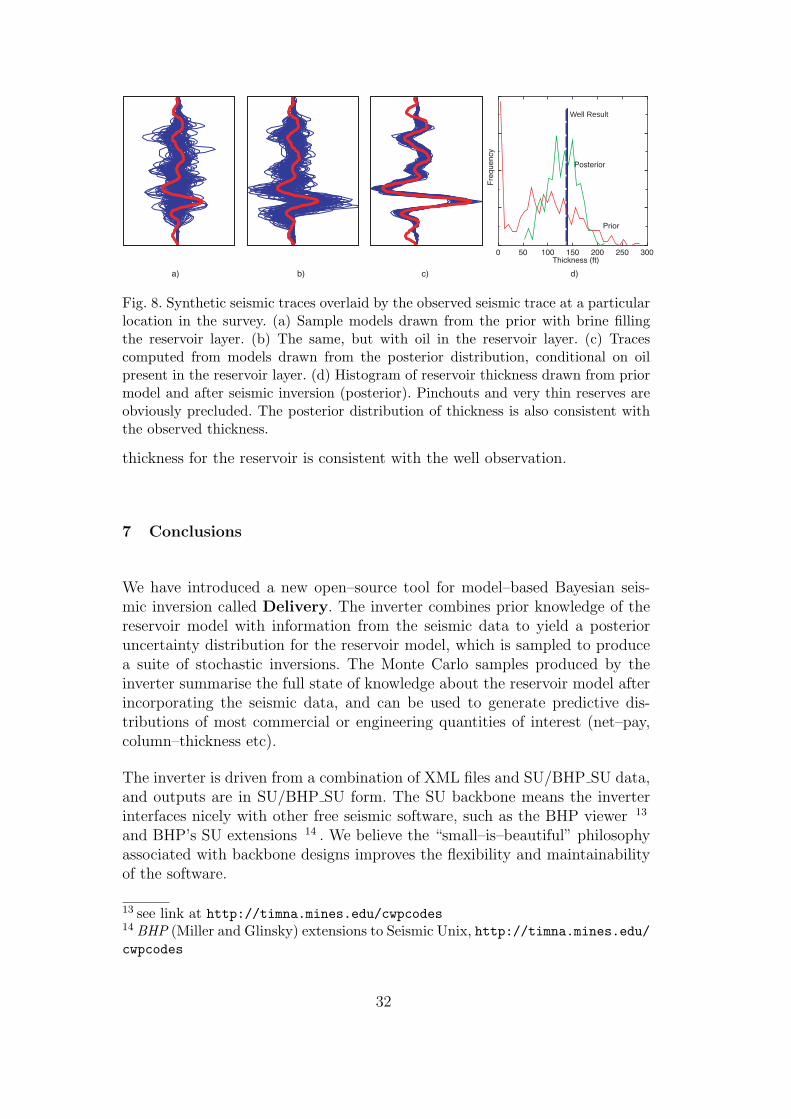
We expect in the near future to publish several extended papers focussed on theinversion of some real field data using Delivery and the workflow of developingthe prior. For the moment, we will confine our discussion to a simple test for anactual field, shown in figure 8. This is a ’test’ inversion at the well location. An8–layer model for a set of stacked turbidite sands has been built with provenhydrocarbons in the second–bottom layer. The sands are quite clean and havehigh porosities (≈ 30%), so the effects of Gassman substitution are very strongin the reservoir layers. The layers are constructed from log analysis, but theirboundaries are set to have a broad prior uncertainty around the 10-15ms range.Low net–to–gross layers (NG < 0.1) are often set as pure shales (NG = 0) togkeep the model dimensionality down. The prior for fluid type (brine:oil) is setas 50:50, as in the previous example.

The inversion at the well location not only confirms the presence of oil (>80% probability) but also demonstrates that the posterior distribution of layer

31

Well Result

Fig. 8. Synthetic seismic traces overlaid by the observed seismic trace at a particularlocation in the survey. (a) Sample models drawn from the prior with brine fillingthe reservoir layer. (b) The same, but with oil in the reservoir layer. (c) Tracescomputed from models drawn from the posterior distribution, conditional on oilpresent in the reservoir layer. (d) Histogram of reservoir thickness drawn from priormodel and after seismic inversion (posterior). Pinchouts and very thin reserves areobviously precluded. The posterior distribution of thickness is also consistent withthe observed thickness.

thickness for the reservoir is consistent with the well observation.

7 Conclusions

We have introduced a new open–source tool for model–based Bayesian seis-mic inversion called Delivery. The inverter combines prior knowledge of thereservoir model with information from the seismic data to yield a posterioruncertainty distribution for the reservoir model, which is sampled to producea suite of stochastic inversions. The Monte Carlo samples produced by theinverter summarise the full state of knowledge about the reservoir model afterincorporating the seismic data, and can be used to generate predictive dis-tributions of most commercial or engineering quantities of interest (net–pay,column–thickness etc).

The inverter is driven from a combination of XML files and SU/BHP SU data,and outputs are in SU/BHP SU form. The SU backbone means the inverterinterfaces nicely with other free seismic software, such as the BHP viewer 13

and BHP’s SU extensions 14 . We believe the “small–is–beautiful” philosophyassociated with backbone designs improves the flexibility and maintainabilityof the software.

13 see link at http://timna.mines.edu/cwpcodes14 BHP (Miller and Glinsky) extensions to Seismic Unix, http://timna.mines.edu/cwpcodes

32

The authors hope that this tool will prove useful to reservoir modellers workingwith the problem of seismic data integration, and encourage users to helpimprove the software or submit suggestions for improvements. We hope thatthe newer ideas on probabilistic model–comparison and sampling (vis–a–visthe petroleum community) prove useful and applicable to related problems inuncertainty and risk management.

Acknowledgement

This work has been supported by the BHP Billiton Technology Program.

References

Abrahamsen, P., et al., 1997. Seismic impedance and porosity: support effects.In: Geostatistics Wollongong ’96. Kluwer Academic, pp. 489–500.

Abramowitz, M., Stegun, I. A., 1965. Handbook of Mathematical Functions.Dover.

Andrieu, C. A., Djuric, P. M., Doucet, A., 2001. Model selection by MCMCcomputation. Signal Processing 81, 19–37.

Brooks, S. P., 1998. Markov chain Monte Carlo and its application. The Statis-tician 47, 69–100.

Buland, A., Kolbjornsen, A., Omre, H., 2003. Rapid spatially coupled AVOinversion in the Fourier domain. Geophysics 68 (3), 824–83.

Buland, A., Omre, H., 2000. Bayesian AVO inversion. Abstracts, 62nd EAGEConference and Technical Exhibition, 18–28See extended paper at http:

//www.math.ntnu.no/~omre/BuOmre00Bpaper.ps.Castagna, J. P., Backus, M. M. (Eds.), 1993. Offset-dependent reflectivity –

Theory and practice of AVO Analysis. Society of Exploration Geophysicists.Chu, L., Reynolds, A. C., Oliver, D. S., Nov. 1995. Reservoir Description from

Static and Well–Test Data using Efficient Gradient Methods. In: Proceed-ings of the international meeting on Petroleum Engineering, Beijing, China.Society of Petroleum Engineers, Richardson, Texas, paper SPE 29999.

Cohen, J. K., Stockwell, Jr., J., 1998. CWP/SU: Seismic Unix Release 35: a freepackage for seismic research and processing,. Center for Wave Phenomena,Colorado School of Mines, http://timna.mines.edu/cwpcodes.

Denison, D. G. T., et al., 2002. Bayesian Methods for Nonlinear Classificationand Regression. Wiley.

Deutsch, C. V., 2002. Geostatistical Reservoir Modelling. Oxford UniversityPress.

Eide, A. L., 1997. Stochastic reservoir characterization conditioned on seismicdata. In: Geostatistics Wollongong ’96. Kluwer Academic.

33

Eide, A. L., Omre, H., Ursin, B., 2002. Prediction of reservoir variables basedon seismic data and well observations. Journal of the American StatisticalAssociation 97 (457), 18–28.

Eidsvik, J., et al., 2002. Seismic reservoir prediction using Bayesian integra-tion of rock physics and Markov random fields: A North Sea example. TheLeading Edge 21 (3), 290–294.

Gelman, A., Carlin, J. B., Stern, H. S., Rubin, D. B., 1995. Bayesian DataAnalysis. Chapman and Hall.

Gilks, W., Richardson, S., Spiegelhalter, D., 1996. Markov Chain Monte Carloin Practice. Chapman and Hall.

Gunning, J., 2000. Constraining random field models to seismic data: gettingthe scale and the physics right. In: ECMOR VII: Proceedings, 7th Europeanconference on the mathematics of oil recovery, Baveno, Italy.

Gunning, J., 2003. Delivery website: follow links from http://www.

petroleum.csiro.au.Gunning, J., Glinsky, M., 2004. Delivery: an open-source model-based Bayesian

seismic inversion program. Computers and Geosciences 30 (6), 619–636.Gunning, J., Glinsky, M., 2006. WaveletExtractor: A Bayesian well–tie and

wavelet extraction program. Computers and Geosciences 32, 681–695.Huage, R., Skorstad, A., Holden, L., 1998. Conditioning a fluvial reservoir on

stacked seismic amplitudes. In: Proc. 4th annual conference of the IAMG.http://www.nr.no/research/sand/articles.html.

Koontz, R. S. J., Weiss, B., 1982. A modular system of algorithms for uncon-strained minimization. Tech. rep., Comp. Sci. Dept., University of Coloradoat Boulder, Steve Verrill’s Java translation at http://www1.fpl.fs.fed.

us/optimization.html.Leguijt, J., 2001. A promising approach to subsurface information integration.

In: Extended abstracts, 63rd EAGE Conference and Technical Exhibition.Malinverno, A., 2002. Parsimonious bayesian Markov chain Monte Carlo inver-

sion in a nonlinear geophysical problem. Geophysical Journal International151, 675–688.

Mavko, G., Mukerji, T., Dvorkin, J., 1998. The Rock Physics Handbook. Cam-bridge University Press.

Oliver, D. S., 1996. On conditional simulation to inaccurate data. Mathemat-ical Geology 28, 811–817.

Oliver, D. S., 1997. Markov Chain Monte Carlo Methods for Conditioning aPermeability Field to Pressure Data. Mathematical Geology 29, 61–91.

Omre, H., Tjelmeland, H., 1997. Petroleum Geostatistics. In: GeostatisticsWollongong ’96. Kluwer Academic.

Phillips, D. B., Smith, A. F. M., 1996. Bayesian model comparison via jumpdiffusions. In: Markov Chain Monte Carlo in Practice. Chapman and Hall.

Raftery, A. E., 1996. Hypothesis testing and model selection. In: Markov ChainMonte Carlo in Practice. Chapman and Hall.

Storn, R., Price, K., 1997. Differential evolution – a simple and efficient heuris-tic for global optimisation over continuous spaces. Journal of Global Opti-

34

mization 11, 341–359.Tarantola, A., 1987. Inverse Problem Theory, Methods for Data Fitting and

Model Parameter Estimation. Elsevier Science Publishers, Amsterdam.

35

Appendices

Appendix 1: Typical computation of effective rock properties

Here we illustrate how the effective rock properties for a single layer might becomputed from a full suite of fundamental model parameters (equation (1))for the layer.

• Compute the brine+matrix density

ρsat,b = φsρb + (1 − φs)ρg. (43)

• Compute the associated moduli

µsat,b = ρsat,bv2s,s (44)

Msat,b = ρsat,bv2p,s (45)

Ksat,b = Msat,b −4

3µsat,b (46)

µsat,fl = µsat,b (47)

• Use the fluid properties to compute Kb = ρbv2p,b and Kh = ρhv

2p,h, and then

Kfl = (Sh

Kh

+1 − Sh

Kb

)−1

• Using literature values of Kg, compute Ksat,fl using equation (13). This comesout to be

Ksat,fl = Kg/

1 +

[

1

φs

(

1

Kg/Kfl − 1− 1

Kg/Kb − 1

)

+1

Kg/Ksat,b − 1

]−1

(48)

This equation has regions of parameter space with no positive solution (of-ten associated with, say, small φ). The forward model must flag any set ofparameters that yield a negative Ksat,fl and furnish a means of coping sanelywith such exceptions. The same remark applies to equations (46) and (51)below.

• Compute the new effective density

ρsat,fl = (1 − φs)ρg + φs(Shρh + (1 − Sh)ρb),

• Compute also the new effective p–wave modulus from

Msat,fl = Ksat,fl +4

3µsat,fl

36

• Compute the impermeable–rock moduli

µm = ρmv2s,m (49)

Mm = ρmv2p,m (50)

Km = Mm − 4

3µm (51)

• Mix the fl–substituted permeable rock with the shale properties using therock–mixing Backus averaging formula (9). Compute also the mixed densityfrom (10).

• From the mixed rock, back out the velocities vp,eff = (Meff/ρeff)1/2, and

vs,eff = (µeff/ρeff)1/2.

Appendix 2: Error sampling rates

When comparing synthetic seismic traces to co–located actual seismic, it is aquestion of some nicety as to what rate of sampling of the difference trace mustbe applied to quantify the error between the two. It is trivial to show that if arandom process has, eg. a Ricker-2 power spectrum (i.e. ∼ f 2 exp(−(f/fpeak)

2)),then 95% of the spectral energy in the process can be captured by samplingat times

∆Ts = 0.253/fpeak, (52)

where fpeak is the peak energy in the spectrum (and often about half of thebandwidth). Most practical seismic spectra will yield similar results.

The sampling rate in equation (52) is about 2 times the Nyquist rate associatedwith the peak frequency. If the error is acquired with a faster sampling ratethan this, adjacent error samples will be strongly correlated and the errorterm will become large. Since the error covariance is unknown, and bearingin mind that we seek an error measure corresponding to a maximum numberof “independent” data points, we use the rate given by equation (52) andmodel the error points as i.i.d. values. The peak frequency fpeak is estimatedat initialisation from the FFT spectrum of the wavelet.

Appendix 3: Mode–location starting points

The location, characterisation, and enumeration of local modes in the posteriordistribution is performed by a loop over a set of strategically chosen starting

37

points in the model parameter space. Since one of the major functions of theprior distribution is to exclude improbable posterior modes, it makes sense tobase the choice of starting points on the prior distribution.

The fundamental variables associated with multi–modality are the layer times,in that the posterior likelihood surface is frequently oscillatory in the layertimes. Convergence to a secondary or minor solution is usually called loop–skipping, and may or may not be desirable. In situations where loop skippingmay be permissible or even desirable, the prior uncertainty on the layer timesis usually set to be quite broad, as these secondary solutions may be feasible.Convergence to these solutions can then be prompted by setting the initial layertimes fed to the minimisation routine at values likely to be within the basinof attraction of the desired solution. The hueristic method used for definingthese starting points is as follows:

Form a set of starting configurations, for each fluid state, by:

(1) Forming an approximate multi–Gaussian posterior distribution for theproperties by updating the prior to account for any isopach constraintsand the depth consistency requirement. This posterior is characterised bythe mean m and covariance C. Recall that the layer times are the firsti = 1 . . . (n + 1) elements in the vector m. Fix all non-time parametersi = n + 2 . . . at the values in m.

(2) From this posterior, compute the expected layer time thickness ∆ti, layertime uncertainties σti and layer time thickness uncertainty σ∆ti , from

∆ti = mi+1 − mi (53)

σ2ti

= Ci,i (54)

σ2ti+1

= Ci+1,i+1 (55)

σ2∆ti

= Ci,i + Ci+1,i+1 − 2Ci,i+1. (56)

(3) Now, if σ∆ti/∆ti > 0.5, this amounts to a ≈ 5% chance of the layerpinching out (∆ti < 0) before taking into account the seismic, so this islikely enough to warrant investigation. The starting points

t′i =σti+1

mi + σtimi+1

σti+1+ σti

(57)

t′i+1 = t′i − 2ǫFD (58)

are then used as suitable starting times for the times ti, ti+1. The remain-ing times tj, j 6= i, i + 1 are set at the posterior means tj = mj. If morethan one layer is potentially pinched out, we form a set of starting pointsby looping over the set of potentially–pinched–out layers, and setting onlyone of these layers at a time to the pinched–out starting configuration justdescribed, with remaining times at the values in m.

38

Appendix 4: An Independence Sampler

For each fixed fluid combination k, a successful location of a mode in thefull parameter space will produce a “maximum likelihood” vector mkj

and

local covariance Ckj, by successive Newton iterates (equations (33)–(37)). Here

the index j runs over the set of distinct modes we have found for each fluidcombination by starting from separated starting points, as per Appendix 3 (inmany cases there will be only one). To save notational baggage, we will use khenceforth to mean kj - the context makes the meaning clear.

The Laplace approximation to the mode posterior marginal likelihood is formedby assuming the posterior surface is fully Gaussian, centred at the maximum–likelihood point, and characterised by the covariance Ck. Integrating over allthe model parameters then gives the marginal probability to be proportionalto

qk ∼ (2π)dmk |Ck|1/2Π(mk|S), (59)

where the posterior Π is evaluated as per (27,28), and the determinant anddimension–varying terms in (28) are carefully retained.

A full independence sampler can then be implemented using a Metropolis Hast-ings method. With the chain in mode k, with model vector mk, we propose anew mode k′ with probability ∼ p′k, whose new model vector m′

k is drawn fromq(m′

k′) = N(m′

k′|m′

k′ , Ck′). We accept this candidate with the usual probability

α = min(1,Π(m′

k′|S)pkq(mk)

Π(mk|S)pk′q(m′

k′), (60)

or leave the state of the chain unchanged. This method has have somewhatmixed success - it is perfect when drawing from the prior (since the prior ismulti–Gaussian), but is susceptible of being trapped in particularly favourablestates for long periods when the posterior departs sharply from Gaussianity.Further, any thick tails in the posterior density are not likely to be exploredby the proposal density, since it has compact Gaussian tails. The proposaloverdispersion recommended by Gelman (Gelman et al., 1995, Ch. 11) doesnot work well, since the dimensionality is so high that even mildly overdisperedt–distributions dramatically reduce the acceptance rates, even when samplingfrom the prior.

It has proven useful to implement an approximate sampler where the modesare proposed from the posterior marginal (∼ qk′) with normal approximationsat each mode (q(m′

k′) = N(m′

k′|m′

k′ , Ck′), and mandatory acceptance (α = 1).

39

Such candidates appear to very rarely produce unlikely χ2 values for the seismicand isopach likelihoods.

Appendix 5: Modified SU trace formats for properties

5.1 Model–prior trace formats

The local prior information for the inversion at each trace is communicatedto the inversion code by a SU data set with a set of traces on a pattern andordering that matches the SU seismic data set exactly. The xml Modelparame-ters.xml file which sets up the inversion will specify which prior quantities varyon a trace-by–trace basis, and the block indices k at which they are located.Suppose there are Np properties which vary, and there are Nl layers. The valuefor property k in layer l is then the (l + (k − 1)Nl)th float value in the currenttrace of prior data. There are some special rules as well

• The layer times must always be present in the prior trace, and they mustalways be the last block (k = Nk). Further, one additional float value isappended for the base time of the last layer tbase).

• All values are expected to be positive, and are converted to positive numbersif not. The value -999.0 signifies a “bad value”, and will be ignored (thedefault prior will then apply)

• All times are in milliseconds.• Layers can be effectively suppressed from the model by providing the isopach

constraint ∆Z = N(0, 0) (see eqn (26)), either from the XML or the modeltraces file for some subset of traces. If this is supplied, the layer is deemed in-active. This is advantageous when a layer is known to permanently pinchoutin some region. Any model reduction help in speeding up the inversion.

5.2 Stochastic trace outputs

Delivery will write stochastic samples from the posterior to the requestedoutput file in a very similar format to the model–prior traces. A sequence ofblocks is written, each of size Nl, and the last block of Nl + 1 floats is eithertime or depth, as specified by the obvious entry in the ModelDescription.xmlfile. The names of the properties can be written to a single–line ascii file bysupplying -BHPcommand filename to the delivery command line.

Similarly, the deliveryAnalyser program can collate the large statistical ensem-ble produced by the delivery output into a compact set of traces representing

40

either means, standard deviations or quantiles of all the salient quantities ofinterest. The set of property names of the blocks in these summary traces isobtained by adding -BHPcommand filename to the deliveryAnalyser com-mand line.

Appendix 6: Wavelet format

Wavelets are expected to be single trace SU files, with the fields ns, dt and f1set to reflect the number of samples, sampling interval, and starting time of thefirst sample (beginning of precursor). The ns and f1 fields are set so as to makethe wavelet as compact as possible with respect to the tapering, so excessivesamples are discouraged, but the tapering must also be smooth to the first andlast sample. Wavelets generated by the WaveletExtractor code (Gunning andGlinsky, 2006) distributed with Delivery are automatically properly initialized.

Appendix 7: Usage of the code

7.1 Inputs

Typical usage of the delivery inversion code demands 3 input files:

• An XML file ModelDescription.xml specifying the disposition of the lay-ers, the rock and fluid physics, and so meta–information about the su tracescontaining the variable prior information.

• One or two SU files for the seismic data. These will represent near (andpossibly far) offset data.

• An SU file containing the variable prior information.

In distributed systems, the latter two items may refer to named pipes on aunix/Linux system.

A typical inversion would be run with the command% delivery ModelDescription.xml -m prior traces.su -v 3 -PD -o re-

alisations.su -N 1000

which will generate (-N) 1000 realisations per trace and write them (-o) tothe file realisations.su, using the pinchout detection (-PD) BFGS meth-ods described in section 4.1. The prior model (-m) is read from the SU fileprior traces.su. Many other commandline options are available, and can beperused in the code’s SU–style self documentaion.

41

7.1.1 The ModelDescription.xml file

The inversion is chiefly driven by an XML file that specifies the necessary rock–physics, layer descriptions, and information about the seismic. A well formedXML file is crucial to this end, so the file can be created using a schema–driven GUI editor expressly built for the purpose, which is also available at thewebsite. “Help” documentation for the inverter is available through standardmenus. The editor is also capable of creating, running and controlling complexscripts on distributed systems, using a schema for common unix, SU, BHP SUand delivery commands.

The structure of the XML document is controlled by the schema, and themeaning of the various entries is readily inferred by reference to the examplesin the distribution.

Some particular entries in the XML file are worth further explanation

• The attribute “varies areally” may be set to true or false for a certain prop-erty. If true, the quantity in question will vary on a trace–by–trace basis, andis expected to be read in from the SU model file. The “<property indices>”block then will contain an entry “property link” which defines the block ofthe SU model file containing the property (see Appendix 5).

• Various properties may contain the attribute “same as layer above”. Thisis set to true when the property in question should be a replica of thesame property in the layer above. For example, the low–frequency–interval–velocity (LFIV) is usually a coarse scale measure representing an averageacross many layers, so it is best fixed at the same value (or mapped to thesame stochastic variable) for all of the relevant layers. Likewise, the “depth”input is an approximation used to sample from the trend curves, and maysafely be set to the same value for many adjacent thin layers. Prudent useof this attribute helps to reduce the dimensionality of the final model.

• Each “<layer>” entry may have the attribute “synchronise rock matrix” setto true. This is a flag to indicate that any stochastic rock properties of a givenrock type in this layer must be matched to those of the matching rock typein the layer above (for example, the vp, vs and φs of the permeable memberin the two layers is mapped to the same underlying stochastic variable Bythis means, two adjacent layers with matching end–member rocks are madeacoustically indistinguishable but for fluid property differences. Any internalreflections are then due to fluid contrasts, and this feature can then be usedto make the layer boundaries track a fluid interface.

• Linear trend curves are of form vs = slope × vp + intercept ± sigma. TheGardner-Gardner-Gregory regression curves for impermeable rocks are of

form ρ = factor × vexponentP ± sigma.

• The “<output>” block has the following useful flags.· “<density ordering>” is set to one of full/partial/none, with the meanings

42

as described in section 2.2.2.· “<realisation number header field>” denoted the SU header word used to

store the realisation number.· “<master depth layer number>” denotes the layer number from which

depths of the other layers will be computed using summations of layerthicknesses (vp,eff× one–way time thickness). The actual depth of the mas-ter layer is the depth variable d in the model vector m.

7.2 Outputs

The inversion code dumps stochastic realisation of the posterior model to aseries of SU traces, so the fastest scan direction in the resulting (large) SU fileis that of the realisation number, which defaults to the mark header word.Posterior analysis of the simulations is performed with a second program de-

liveryAnalyser, which can form various statistical quantities of interest, syn-thetic seismic traces, and blocked layer maps of the simulations. Some of thesalient quantities of interest include

• All the basic model variables in m of equation (3).• Fluid type.• Effective layer properties such as vp,eff, ρeff, Zeff (impedance).• Effective reflection coefficients for each stack at the layer top.• Both a normalised and full χ2 variable indicating the degree of match with

the seismic, from equation (25)).

χ2seismic ≡ ferror

∑

error–sampling points

(Ssyn − S)2/2σ2s (61)

χ2seismic,normalised ≡

χ2seismic

Nerror-sampling-points

(62)

• Thickness (one–way time–thickness × vp,eff.• Net sand (net sand = thickness ×NG).• Net hydrocarbon (Net sand × porosity × saturation).

Like delivery and SU programs, the program has self documentation, butsome typical analysis of a suite of realisations realisation.su might be

(1) deliveryAnalyser -i realisations.su -p-ascii t 6 | ascii–graphing–

program

Print the time of layer 6 from succesive realisations out as an ascii streamand graph it.

(2) cat realisations.su |deliveryAnalyser --mean NG 6

Print a series of realisation averages of NG in layer 6, one for each tracelocation.

43

(3) cat realisations.su |deliveryAnalyser --filter fluid type = 1 4 --

trace--filter ’fldr>1234’ --mean NG 6

Print a series of realisation averages of NG in layer 6, one for each tracelocation, but only for realisations with oil (fluid type=1) in layer 4, andfor the traces with fldr>1234 (note the shell protection).

(4) deliveryAnalyser -i realisations.su --histogram net-sand 6 --trace-

-filter ’fldr=34,tracf=12’ | ascii–graphing–program

Print a histogram of net-sand (NG×thickness) in layer 6 at the specifiedlocation.

(5) deliveryAnalyser -i realisations.su -s 4 5 R near wavelet.su |suswapbytes | suximage

Produce a synthetic near–stack seismic from the model realisations overthe time interval 4-5 seconds from the wavelet wavelet.su and displaythis on a little endian machine (all the java codes wrote big–endian SUfiles).

Appendix 8: Incorporation of Floating Grain models into Delivery

A lithological phenomenon that affects some kinds of reservoir rocks is thepresence of granular material in the pore space that does not support therock matrix, though it does reduce the porosity and permeability. We assumeadequate rock–phyics regressions for the relevant facies can be built from logdata samples unaffected by such material. Delivery has been extended to modelthese effects along the following lines.

8.1 Floating grain effects

The effects of floating grains in the rock matrix can be taken into accountusing regressions curves of the form

φ =−φflt

1 − fc

+ aφ + bφZeff + ǫφ (63)

vp = ap + bp(φflt + (1 + g)φ) + ǫp (64)

where fc is the capture fraction (volume of second material taken into sup-porting matrix divided by total secondary material). The effective stress de-pendence appears is some well chosen function Zeff, with available data, whichmay be, e.g. of form Zeff = (1 − exp(−P/P0)). The ǫ terms are noise terms.

These forms are chosen as linearisations of the nonlinear Gassman model

44

vp(φ, φflt) =

{

Kg

ρg + (ρb − ρg)φ

(

3(1 − νm)

1 + νm

β(φ, φflt)

+(1 − β(φ, φflt))

2

(φ + φflt)((Kg/Kf (φ, φflt)) − 1) + 1 − β(φ, φflt)

)}1/2

(65)

about a mean porosity φ and φflt = 0, which arises from the following strongassumptions. The grains are assumed to have the same properties as the matrix(same material – subscript g), and variations in the Poisson’s ratio νm withφ and φflt are neglected. We model the rock beta behaviour as a function ofstructural porosity φs = φ + φflt as

β(φ, φflt) = (1 − (φ + φflt)/φ0)λ, (66)

and the ’effective fluid’ modulus by the Reuss average of floating grains andbrine moduli

Kf (φ, φflt) =

(

φ/Kb + φflt/Kg

φ + φflt

)−1

. (67)

The parameters λ, φ0 can be obtained by a nonlinear regression of the clean-rock {vp, φ} data using φflt = 0 in the above formulation (equation 65), using

known values for Kg, ρg, ρb etc. The critical porosity φ0 is very likely to be inthe range 0.4−0.45. If a value for Poisson’s ratio representative of the averageporosity is chosen (e.g. νm = 0.15), the dominant unknown in equation (65)is λ, which can be simply regressed for. Note that using an assumed value forνm (e.g. νm = 0.15), appropriate for the average of data porosity will not yieldthe correct pure quartz velocity vp(0, 0) since a pure quartz Poisson’s ratio iscloser to 0.07.

The slope and intercept terms in eqn (64) emerge naturally from the lineari-sation of the nonlinear fit to (63) of clean rock data.

We define (1 + g) by

(1 + g) ≡ ∂vp(φ, φflt)

∂φ

∣∣∣∣∣φ=φ,φflt=0

/∂vp(φ, φflt)

∂φflt

∣∣∣∣∣φ=φ,φflt=0

(68)

and sufficiently accurate numerical values for the derivatives are most simplyobtained by finite differences.

45

8.2 Recommended methodology

A possible regression methodology is as follows. For clean rock data,

• Assume Kg, Kb, ρg, ρb, νm

• Compute the mean porosity φ• Fit the vp data for the non-linear parameters λ, φ0

• Compute the bp, bp(1+g) coefficients of eqn (64) from the derivative expres-sions in the Appendix at the mean porosity. Then ap = vp(φ, 0)− bp(1+g)φ.

• For this clean rock data, here are no φflt terms in (63) and (64), so fitthe loading–behaviour data to get the coefficients aφ, bφ and residuals RMS

σǫφ=

√

〈ǫ2φ〉

• Fit the linearised velocity trend data to get the coefficients ap, bp, and resid-

uals RMS σǫp=

√

〈ǫ2p〉

Now, for each group of float-polluted well data 15 (i.e. which can be modelledwith an common effective φflt)

• Refit the two linearised trends, using different intercepts:

φ = a′

φ + bφZeff + ǫφ (69)

vp = a′

p + bp(1 + g)φ + ǫp (70)

We then compute the common float fraction and capture ratio:

φflt = (a′

p − ap)/bp (71)

fc = 1 − φflt/(aφ − a′

φ) (72)

A simple check of the theory is to confirm the new regressions have the sameslope as the clean rock data.

8.3 Conversion to Delivery formats

For use in Delivery, augmented regression relationships of the form

vp = Ap + Bpd + CpLFIV + Dpφflt + ǫ′p (73)

φ = Aφ + Bφvp + Cφφflt + ǫ′φ (74)

will be used, using the existing notation in Delivery documents. The shearrelation is unchanged. The pressure dependence will be effected by taking the

15 Regressions for the data with floating grains can be performed using EM(Expectation-Maximisation) techniques, a possible future development

46

loading depth d → Zeff (e.g. (1 − exp(−P/P0))) computed from e.g. basinmodelling (use the depth rock curves entry in the XML, to distinguish frommodel depth). The LFIV will be dropped by setting Cp = 0. Approximateconversion to this Delivery–style form of the coupled regression can be obtainedwith

Ap = ap + bp(1 + g)aφ (75)

Bp = bpbφ(1 + g) (76)

Dp = bp(1 − 1 + g

1 − fc

) (77)

Aφ =− ap

bp(1 + g)(78)

Bφ =1

bp(1 + g)(79)

Cφ =− 1

1 + g(80)

σ′

ǫp=

√

σ2ǫp

+ (bp(1 + g))2σ2ǫφ

(81)

σ′

ǫφ=

σǫp

bp(1 + g)(82)

Numerical Example

8.4 Rock trends

We use the loading depth term Zeff = (1 − exp(−P/800PSI)) for the loadingregressions, which is input to Delivery as the parameter depth rock curves.At a particular location of interest, Zeff = 0.976 at P = 3000 PSI, roughlyaround the depth 11000ft.

Modelling loading behaviour in a certain petroleum province yields the follow-ing estimates for shales and sands.

8.4.1 Shales

The loading behaviour for non–reservoir rocks (shales) has also to be convertedto use the Zeff variable. For simplicity, we took typical velocities from theexisting depth–based trends, then set Bp = 0 to yield

vp = 10500 ± 470ft/s (83)

47

ρm = 0.278v0.234p ± 0.027gm/cc (84)

vs =−2333 + 0.678vp ± 280ft/s (85)

8.4.2 Sands

The fits here are:

φ = 1.10 − 0.88(1 − exp(−P/800PSI)) − 1.54φflt ± 0.0024 (86)

vp = 18717 − 32100φ − 31060φflt ± 750ft/s (87)

vs = = −2774 + 0.77vp ± 240ft/s (88)

The coefficients we require are read off as ap = 18717, bp = −31060, aφ = 1.1,bφ = −0.88, fC = 0.33 and (1 + g) = 1.033. Coefficients for use in Delivery arecomputed from equations (75)– (82) as Ap = −16576, Bp = 28235, Dp = 16830,Aφ = 0.583, Bφ = −3.11 × 10−5, Cφ = −0.968. The shear coefficients areAs = −2774, Bs = 0.77.

From the estimated noise RMS values σǫφ= 750 and σǫp

= 0.0024 we computeσ′

ǫp≈ 700ft/s and σ′

ǫφ≈ 0.02 as working guesses.

8.5 Model system

Consider a 2–layer shale–seal:sand system, where the sand layer is initiallymodelled as clean (NG ∼ N(1, 0)). The well logs used to construct the priorhave some clean rocks (no floating grains) and rocks with floating contentof around 5%. To model the inferability of the float fraction, we constructsynthetic seismic truth–case stacks for near and far stack angles of a few degreesand about 30◦, using a truth case model with 5% float, and all other parametersat the most likely values from the trends. Fig 9 illustrates the system, withtruth-case plus posterior near and far synthetics from the posterior of case iii)we describe shortly.

For inversion, the prior on floating fraction is taken as N(0, 0.052), and weattempt to compute the posterior floating fraction fraction from 3 cases: i)NG fixed at 1, near–stack only, ii) (NG ∼ N(1, 0.22), near–stack only, and iii)(NG ∼ N(1, 0.22), near and far stacks.

For case i), figs. 10– 12 shows 3 possible forms of the prior – varied for illustra-tive purposes – on which we superpose the original log data, which illustrateshow the floating grain effect smears out the regional prior. The actual priorused int he inversion cases coincides with the inset (c).

48

1.8

1.9

2.0

2.1

-0.02 -0.01 0 0.01 0.021.8

1.9

2.0

2.1

-0.02 -0.01 0 0.01 0.02

SAND

SHALE

Near Far

Fig. 9. Two–layer model system with truth case (thick red) seismic traces and syn-thetics from the posterior (black) for the inversion case iii) described in the text.The absolute noise level is set at 0.0025 for both stacks.

0.050.100.150.200.250.300.358×1039×1031.0×1041.1×1041.2×1041.3×1041.4×104

0.05 0.10 0.15 0.20 0.25 0.30 0.358 ×103

9 ×103

1.0 ×104

1.1 ×104

1.2 ×104

1.3 ×104

1.4 ×104

Fig. 10. This and figs. 11 and 12: three ’pedagogic’ priors for velocity versus porosityin pure sand layer. Clean well data points (+) and float-polluted well data points (*)plotted on all three graphs: dots (.) are draws from model prior. (a) Prior constructedwith artificially narrow σφ = 0.002, showing how parameters arise from a clear 50:50mixture of ’clean–rock regression’ points and an elliptical smear from the effects ofthe floating grains. The clean rock trend is obviously far too narrow to embrace theclean well (+) measurements, but the ’clean trend’ is clearly visible and centred.

8.6 Inversion Analysis of Posteriors

8.6.1 Fixed NG, single stack

Figure 13 shows salient scatterplots of properties of the sand layer before andafter inversion. The peak–signal to noise ratio is set at about 6:1.

49

0.05 0.10 0.15 0.20 0.25 0.30 0.359 ×103

1.0 ×104

1.1 ×104

1.2 ×104

1.3 ×104

1.4 ×104

Fig. 11. Illustrative prior (b): prior drawn from clean rocks only (float–fraction∼ N(0, 0)), with realistic σφ = 0.02. The tails of the distribution do not containthe floating grain data comfortably. Clean well data points (+) and float-pollutedwell data points (*), dots (.) are draws from model prior.

0.05 0.10 0.15 0.20 0.25 0.30 0.359 ×103

1.0 ×104

1.1 ×104

1.2 ×104

1.3 ×104

1.4 ×104

Fig. 12. Illustrative prior (c): actual prior with float–fraction distributed as∼ N(0, 0.052). Only a few measurements appear to lie at the periphery of the distri-bution, but the mixture character is not as clear to the eye as in fig. 10. Clean welldata points (+), float-polluted well data points (*), dots (.) are draws from modelprior.

8.6.2 Free NG, single stack

Figure 14 shows salient scatterplots of properties of the sand layer after inver-sion, where the model has additional net–to–gross freedom free in the priorNG ∼ N(1, 0.22).

50

phi (sand porosity)

phi (sand porosity) vp(sand) (ft/s)

vp(sand) (ft/s)

t(ms)

t(ms)

R_near

R_near

rho_s (

gm

/cc)

rho_s (

gm

/cc)

float_

fraction

float_

fraction

A B C

D E F

PR

IOR

PO

ST

ER

IOR

0.00 0.05 0.10 0.15 0.20 0.25 0.30 0.350.00

0.02

0.04

0.06

0.08

0.10

0.12

0.14

2.1

2.2

2.3

2.4

2.5

2.6

1970 1980 1990 2000 2010 2020 2030-0.2

-0.1

0.0

0.1

0.2

0.00 0.05 0.10 0.15 0.20 0.25 0.30 0.350.00

0.02

0.04

0.06

0.08

0.10

0.12

0.14

2.1

2.2

2.3

2.4

2.5

2.6

1970 1980 1990 2000 2010 2020 2030

-0.1

-0.2

0.0

0.1

0.2

8000 10000 12000 14000

8000 10000 12000 14000

Fig. 13. Scatterplots from prior distribution (top row) and posterior (bottom row)for 2–layer model with sand below shale. (A,D) float fraction vs sand porosity. Aperceptible narrowing around the true answer of float fraction=5% is visible. Fewerclean sands are produced in the posterior. (B,E) The velocity (vp) density scat-terplot narrows more obviously. (C,F) The layer–time (t) versus effective reflectioncoefficient Reff is clearly pinned down sharply. As usual, these parameters are mostheavily constrained.

8.6.3 Fixed NG, near+far stack

Inversion using shear data may help narrow down floating grain porositiesbetter, as the shear carries additional information. The far stack for this testcase is set at about 30 degrees (c.f. a few degrees for the near) and the reflectedamplitude is much weaker (AVO effects). The noise level was set at the samevalue as for the far stack.

Figure 15 shows comparable scatterplots to 14.

8.7 Delivery Implementation details

Recall that Delivery works with two versions of the model vector m. Thevector m has a fully Gaussian prior, with no truncations or restrictions onvalues. The physical model vector m′, which is used in the forward modeland its associated likelihoods (seismic, isopachs) is obtained by applying timeorderings and truncations (e.g. of NG or saturations) to m, i.e. m′ = f(m), forsome suitable f . The truncation effectively induces a prior which, for simple

51

0.00 0.05 0.10 0.15 0.20 0.25 0.30 0.350.00

0.02

0.04

0.06

0.08

0.10

0.12

0.14

8 ×103 9 ×103 1.0 ×104 1.1 ×104 1.2 ×104 1.3 ×104 1.4 ×1042.1

2.2

2.3

2.4

2.5

2.6

−0.05 0.00 0.05 0.10 0.150

200

400

600

800

1000

0.00 0.02 0.04 0.06 0.08 0.10 0.12 0.140.3

0.4

0.5

0.6

0.7

0.8

0.9

1.0

floa

t_fr

actio

n

phi vp_s

rho_

eff

float_fractionfloat_fraction

NG

freq

uenc

y

A

C

D

B

Fig. 14. Posteriors from model with loosened NG distribution in prior. (A) float–frac-tion vs sand porosity. (B) The velocity (vp) vs density. (C) Histogram of float–frac-tion from the posteriors of the models with fixed NG = 1 and free NG ∼ N(1, 0.2).No obvious effect on the univariate float–fraction distribution is caused by allowingthe NG to become free: the peaks of the two delta functions are shown with ar-rows. (D) Scatterplot of NG vs float–fraction. Again, no obvious strong correlationappears here, with the density strongest near the truth case values (0.05, 1.0).

properties like NG, is a mixture of a truncated Gaussian distribution and deltafunctions at endpoints.

With the augmented models defined by equations (73) and (74), the linearitymeans the prior is still Gaussian, but the truncation of φflt in m′ must behandled with care. The extra coefficients Dp, Cφ have the effect of placing theprior on inclined ellipsoids in e.g. the {vp, φflt} plane, so pure truncation on φflt

has the effect of smearing the tail of the distribution onto the plane φflt = 0in a direction off the principal axes. This is clearly a poor way to handle theprior. Fig 16 shows a scatter plot of points produced from a prior constructedin this naive way, with the obvious artifacts. A more reasonable way to handlethe truncation is with the mappings (only for φflt < 0):

v′

p = vp − Dpφflt (89)

φ′ = φ + Bφ(v′

p − vp) − Cφφflt (90)

52

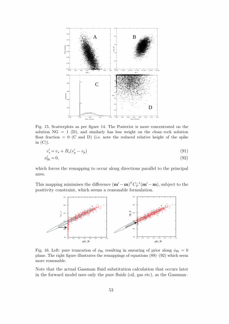
0.00 0.05 0.10 0.15 0.20 0.25 0.30 0.350.00

0.02

0.04

0.06

0.08

0.10

0.12

0.14

8 ×103 9 ×103 1.0 ×104 1.1 ×104 1.2 ×104 1.3 ×104 1.4 ×1042.1

2.2

2.3

2.4

2.5

2.6

−0.05 0.00 0.05 0.10 0.150

200

400

600

800

1000

0.00 0.02 0.04 0.06 0.08 0.10 0.12 0.140.3

0.4

0.5

0.6

0.7

0.8

0.9

1.0

float_fraction float_fraction

vp_s

rho_

eff

floa

t_fr

actio

n

phi_s

NG

freq

uenc

y

C

D

A B

Fig. 15. Scatterplots as per figure 14. The Posterior is more concentrated on thesolution NG = 1 (D), and similarly has less weight on the clean–rock solutionfloat–fraction = 0 (C and D) (i.e. note the reduced relative height of the spikein (C)).

v′

s = vs + Bs(v′

p − vp) (91)

φ′

flt = 0, (92)

which forces the remapping to occur along directions parallel to the principalaxes.

This mapping minimises the difference (m′−m)T C−1P (m′−m), subject to the

positivity constraint, which seems a reasonable formulation.

0.00 0.02 0.04 0.06 0.08 0.10 0.12 0.14 9 ×10 3

1.0 ×10 4

1.1 ×10 4

1.2 ×10 4

1.3 ×10 4

1.4 ×10 4

phi_flt phi_flt

vp_s

vp_s

0.00 0.02 0.04 0.06 0.08 0.10 0.12 0.14 9 ×10 3

1.0 ×10 4

1.1 ×10 4

1.2 ×10 4

1.3 ×10 4

1.4 ×10 4

Fig. 16. Left: pure truncation of φflt resulting in smearing of prior along φflt = 0plane. The right figure illustrates the remappings of equations (89)–(92) which seemmore reasonable.

Note that the actual Gassman fluid substitution calculation that occurs laterin the forward model uses only the pure fluids (oil, gas etc), as the Gassman–

53

like effect of the floating grain presence is implicitly accounted for by thefloating–grain terms in the modified regressions.

8.8 Inputs/Outputs

The prior distribution of the floating grain volume fraction is specified on alayer–basis for the reservoir rock, like, say, the saturation of a hydrocarbontype. It’s default is N(0, 0), so the model reduces to the standard model bydefault. Outputs will be the modified porosity (1−SL)φs (actual fluid porosity)and the additional field fL. The SU header word duse will encode output fileformat variations for compatibility with older models (it is rarely used, anddefaults to zero).

Appendix 9: Vertical model–stacking functionality

An additional feature added to Delivery since the published paper is the ca-pacity to vertically stack models, which is a clandestine way to study modelswhere transverse correlations between parameters at different spatial locationscan be important, or at least more tightly constrained than the allowable(regression-error) variations in the regional rock curves.

The idea here is that the coupled inversion at two or more separate spatial loca-tions – where there exists significant transverse correlation of layer properties– can be effected by stacking several models on top of one another at a singlespatial location, and including coupling terms for the likelihood which connectproperties in arbitrarily different layers. The idea is illustrated in figure 17.

The seismic data from the several locations is “stacked” in a similar way. Con-sider a “two–stack” case for example: a three-layer model with time–windowof interest t ∈ [1, 1.5]s, can be stacked into the total interval t ∈ [1, 2.5] withlocation 1 in [1, 1.5]s and location 2 in [2, 2.5]s. A suitable buffering time in-terval (in this case [1.5, 2]s) is used between the two packages. Dummy shalepackages can also be inserted if desired.

The user must specify a set of one or more layer mappings, each of whichspecifies a base layer and one or more target layers via an xml entry like<mapping>1:5,6</mapping> which has base layer=1 and target layers = 5,6.These then enable the coupling of properties between the base layer and thetarget layers. This is a quite general form – in simple two–location modelsthere is only one target layer for each base layer.

Functionality to couple the properties p ∈ {vp, vs, φs, ρm, NG, thickness} exists.

54

1

2

3

4

5

6

7

8

t

3σt3σt

3σt

coda

precursor

exclusion

window

wavelet

time t

laye

r m

ap

pin

gs

ba

se_

laye

rsta

rge

t_la

yers

Fig. 17. Illustration of construction of a stacked 8–layer model from two 3–layermodels with buffering shale layers. Mappings between comparable layers are shownon the left. To exclude seismic–mismatch coupling effects from the region wherethe two packages join, a seismic–likelihood exclusion–window is constructed, wherethe XML specifies the parameters (start layer=5, end layer=4). The constructedexclusion zone starts from a “safe” distance above the top of the start layer (i.e.including prior time uncertainties and the effect of the wavelet coda) down to a“safe” time below the bottom of the named end layer (using the wavelet precursorand 3 standard deviations of the prior time pick).

For each of these properties, the user provides a between–layers “difference”variance σp (in the same units as the trend curves), and can (optionally) sub-select the set of applicable base layers over which it is desirable to couple theproperty. If the variance σ is small or comparable to the typical errors in theregional curves, the coupled inversion can be expected to give quite differentanswers to inversions carried out independently at each spatial location.

For the properties p ∈ {vp, vs, φs, ρm, NG}, the difference constraint can beabsorbed rigorously in the prior. The extra term in the Gaussian prior exponent(c.f. equation (28), with the fluid–choice subscript k suppressed for simplicity)corresponding to this construction is of form

− log(P (m)) =1

2

∑

properties p

∑

applicablebase layers ip

∑

target layers jip

(mI(p,ip) − mI(p,jip ))2

σ2p

.

(93)

55

where I(p, j) denotes the index of property p, layer j, in m. The RHS in (93)is a quadratic form which we may write as mT C−1

V Sm/2, where CV S is a ma-trix assembled from a sum of block matrix type entries of the general type

(1 −1

−1 1)/σ2

p, inserted in the appropriate rows and columns.

The net effect of this term is that the existing prior specified by the rock–physics curves and time–picks can be simply updated using the usual Bayesianformulas to the new Gaussian prior with parameters

C ′

m = (C−1V S + C−1

m )−1

m′ = (C−1V S + C−1

m )−1C−1m m (94)

Thus, the prior is the same multi–Gaussian expression as equation (28), butwith the modified mean and covariance as per (94). In particular, specificationof “vertical stacking” terms for p ∈ {vp, vs, φs, ρm, NG}, or their modification,does not alter the overall prior probability of the model.

Note that the thickness constraint does not contribute a pure quadratic termthat can be absorbed rigorously into the Gaussian prior. Though we wouldlike to treat all vertical–stacking requirements as part of the prior (and thisis also often true for isopachs), this requires that the normalisation constantsare explicitly available, and these are not analytically available for terms thatdo not appear directly as Gaussian. Hence the vertical–stacking constraintfor thickness is imposed via a likelihood term, very similarly to the isopachconstraint. This means that changes in the vertical–stacking thickness term willalter the underlying probability of a model, just as the isopach and seismic datadoes. For completeness, we write the likelihood from the thickness differenceas

LVSth(m) =1

(2π)dth/2|CVSth|1/2

exp(−1

2

∑

applicablebase layers ip

∑

target layers ji

(∆Zi(m) − ∆Zji(m))2

σ2Zi

). (95)

where CVSth = diag{σ2Zi} contains dth entries, one for each term of the double

sum in the exponent.

A minor complication with this trick of vertical stacking is that the reflectedseismic amplitudes at the interfaces between each “package” of layers willcouple the properties between the top and bottom of adjoining packages, whichis usually undesirable. In this context, the amplitudes at these times are of nointerest, and should be excluded from the inversion. The user has the optionof excluding these using one or more xml entries of typical form

56

<seismic_likelihood_exclusion_range>

<start_layer>5</start_layer>

<end_layer>4</end_layer>

</seismic_likelihood_exclusion_range>

Each such entry defines a time–window where seismic–mismatch terms are notaccumulated in the likelihood equation (25). The window is defined by theinterval

t > tstart layer − 3σtstart layer− |wavelet–coda|

t < tend layer+1 + 3σtend layer− |wavelet–precursor| (96)

where the mean and standard deviations ti and σti are those of the priorpicks of layer times, c.f. section 2.2.1. This definition enables the exclusion–window(s) to track the model over space. Figure 17 illustrates how this works,for a 8–layer model.

A typical XML chunk to perform two–location stacking for the 8–layer modelshown in this figure would be

<stacked_models_info>

<layer_mappings>

<mapping>1:5</mapping>

<mapping>2:6</mapping>

<mapping>3:7</mapping>

</layer_mappings>

<property_difference_std_deviations>

<vp_m applicable_layers="1,3">350</vp_m>

<rho_m applicable_layers="1,3">0.02</rho_m>

<vp_s applicable_layers="2">250</vp_s>

<phi_s applicable_layers="2">0.1</phi_s>

<NG applicable_layers="2">0.1</NG>

<thickness applicable_layers="2">15</thickness>

</property_difference_std_deviations>

<seismic_likelihood_exclusion_range>

<start_layer>5</start_layer>

<end_layer>4</end_layer>

</seismic_likelihood_exclusion_range>

</stacked_models_info>

For convenience, the runtime flag -IVS switches off all the inter–layer couplinginduced by the likelihood term (93), which is convenient for quick comparisons.

57

Appendix 10: Internal fluid–contact modelling

A common scenario in inverting is one in which the vertical sequence of possiblefluids is known from particular fluid contacts observed in wells or inferred frompressure data. Often the relative uncertainty in the contact depth(s) is not largerelative to the layer–depth uncertainties in the inversion, and reflections fromthe fluid contact(s) can be very strong, so using this additional contact datais very useful.

The default operating mode of the inversion uses the supplied fluid probabilitiesto construct an enumerated list of fluid combinations for the entire model,where each combination assumes that layers are completely occupied by thenominated fluid type. In situations where a particular fluid contact intersectsmany different layers across the inversion domain, this style of modelling canbe messy to construct, especially if layers are introduced as a clandestine wayof capturing the fluid contacts.

As an alternative, a simple fluid–contacts inversion mode is supported, wherethe fluid configuration of any layer is determined by specified fluid contacts indepth, and the computed layer–depth using the model velocities, times, andspecified reference depth layer. In this mode, reflections arising from within-layer fluid contrasts are incorporated into the forward model.

In this “contact–mode” inversion, fluid combinations are not enumerated asbefore, rather, the fluid sequence is deterministically computed from a set of1 or more “fluid units”, as depicted in figure 18.

Fluid units satisfy the following rules.

• A fluid unit is a set of contiguous layers, and within a fluid unit there maybe 1, 2 or 3 of the following contacts {gl, go, gb, lo, lb, ob} (oil (o), gas (g),brine (b), low–saturation gas (l)), under usual full–density ordering.

• The set of fluid units must account for all the layers in the model• Storage efficiencies require the total number of contacts from all fluid units

not exceed the total number of layers in the model (in practice a very unlikelyrestriction).

• Two adjacent fluid units must have an impermeable layer at the bottom ofthe upper fluid unit or top of the lower fluid unit. This allows unusual fluidsequences between fluid units, analogous to the ’partial–density–ordering’which models layer sequences not in hydraulic communication

• Fluid units are itemised in the XML in descending depth order• Contacts in each fluid unit specify the upper and lower fluid type, and are

modelled by Gaussian distributions N(Zc, σ2Zc

) whose mean and standarddeviation have default values in the XML, but which may be spatially vari-able via use of the model–prior traces SU file. Contacts contribute a diagonal

58

Fluid unit 1

Fluid unit 2

oil

oil

gas

brine

brine

Seismic trace and reflections

‘go’ contact

‘ob’ contact

‘ob’ contact SHALE

SHALE

SHALE

sublayer 1sublayer 2

Fig. 18. Illustration of concept of fluid units and depth–specified contacts.

elements σ2Zc

to Ck in equation (28) with associated mean Zc inserted in themean vector mk.

• Any layer which can in–principle host a fluid phase inferred from the fluidunits and contacts must specify the fluid in the fluid nameable in each<reservoir endmember> subsection. E.g., if fluid unit 1 identifies a ’bo’ con-tact, all permeable layers spanned by fluid unit 1 must specify the oil nameand saturation (the probability field is ignored). The oil name is expectedto match throughout the fluid unit.

• The fluid unit XML attribute fluid properties synchronised can force thestochastic properties of all hydrocarbon properties within a fluid unit to bemapped from a common underlying variable if set to true. This may be use-ful, if, e.g. similar saturations are expected for, say, gas, in all reservoir lay-ers in the fluid unit. If synchronisation is activated, the XML+model tracesspecification of the uppermost active reservoir layer 16 controls the prior dis-tribution of the fluid properties, even if this layer is above a contact excludingthe fluid.

It is important to note that the supplied fluid probabilities are ignored whenfluid occupations are determined using contacts in this mode.

16 A reservoir layer is defined by a layer with σNG > 0 or NG > 0. Active layersare defined in Appendix 5.1. Note this can vary spatially, so the safest (and leastambiguously documented) option is setting the priors identically in all reservoirlayers.

59

10.1 Upscaling rules

The code populates a variety of layer–effective fields in the output realisations-style SU files, so upscaling rules must be used when there are internal contacts.We use the following:

• velocities vp eff and vs eff are time–thickness weighted averages of sublayervelocities, so subsequent multiplication by the overall layer time–thicknessgives the true layer thickness, i.e. equal to the sum of the thicknesses of thesublayers delimited by contact depths and the layer top/bottom depth.

• density rho eff and saturation S h are thickness weighted averages (thelatter lumping all non–brine fluids), which should give reasonable resultsfor forward calculation of rock mass and hydrocarbon in–place. For mixedhydrocarbon phases, the fields S oil, S lsg, and S gas are probably moreuseful. These last three are phase–specific thickness weighted averages.

10.2 New outputs in the realisations SU file

• Reflection coefficients R near fc, R far fc, which are near and far stackreflection coefficients arising only from fluid contact reflections occurringwithin layers.

• Times t fc of these reflection coefficients, in the same order. No associationof these times with a particular layer, via the layer–slot in the SU file fromwhich they are retrieved, can be made. The layer “owning” the reflectionsmust be determined by comparison with the usual “t” entries.

• Depths d fc of these reflection coefficients, in the same order.• fluid type is output (as before) as an 2 byte integer, with legacy values

0=brine, 1=oil, 2=lsg, 3=gas. These values require only 2 bits of information.For layers split by contact(s), the spare bits of the integer are encoded tocommunicate the sub-layer fluid sequence thus:

Bits 16. . . 13︸ ︷︷ ︸

unused

12,11︸ ︷︷ ︸

A

10,9︸ ︷︷ ︸

B

8,7︸ ︷︷ ︸

C

6,5︸ ︷︷ ︸

D

4,3︸ ︷︷ ︸

E

2,1︸ ︷︷ ︸

F

A = number of internal reflections (= number of sublayers-1)

B = fluid type, sublayer 4, if A>2

C = fluid type, sublayer 3, if A>1

D = fluid type, sublayer 2, if A>0

E = fluid type, sublayer 1, if A>0

F = fluid type of thickest sublayer (”effective” fluid type) (97)

This encoding reduces to the legacy 0,1,2,3 values for layers not split bycontacts.

60

• S oil, S lsg, and S gas. These “effective” saturation components conservecorrect hydrocarbon–phase volume if multiplied by the layer thickness, incases where internal contacts exist. For example, if a oil–brine contact bisectsa layer (in depth), S oil is discounted by 1/2. For contact–free layers, theirvalues are sensible and equal the legacy S h field, for the appropriate phase.

• The Analyser program can now generate net-oil, net-lsg and net-gas,which are correct special cases of net-hydrocarbon, using the S oil, S lsg,and S gas fields described above

Reconstruction of some fraction of the internal detail of the layers is thenpossible using these new or modified fields.

10.3 Example Inversion

Consider the simple 3 layer test problem of figure 19 (see theTests/InverterTests/Simple3LayerContactsTestProblem directory in the distri-bution). The reservoir conditions here are typical of north west shelf Australia,with 30% porosity sands at about 2km TVD. Agnostically, the reference depthlayer is at the top of the model, with a depth standard deviation of 20m.

Fluid unit 1

oil

gas

brine

Seismic traces

‘go’ contact

‘ob’ contact

SHALE

SHALE

~60m

Fig. 19. Simple 3 layer, single fluid unit, 2 contact problem: gas over oil over brine

The 2 contacts are set up with an XML section thus

<fluid_units_and_contacts>

<fluid_unit fluid_properties_synchronised="false">

<top_layer>1</top_layer>

<bottom_layer>3</bottom_layer>

61

<contact>

<type>GO</type>

<depth varies_areally="false">2050</depth>

<sigma_depth varies_areally="false">0</sigma_depth>

</contact>

<contact>

<type>OB</type>

<depth varies_areally="false">2120</depth>

<sigma_depth varies_areally="false">0</sigma_depth>

</contact>

</fluid_unit>

</fluid_units_and_contacts>

Fig. 20 shows synthetics for this model, where the Gassmann fluid effect isvery strong: indeed, fluid–contrasts are stronger than shale–sand contrasts.

2.00

2.05

2.10

2.15

2.20

2.25

2.30

2.00

2.05

2.10

2.15

2.20

2.25

2.30

Fig. 20. Synthetic seismic data for the model of fig. 19 at 200Hz (unrealistic) and80Hz (realistic) bandwidth.

Fig. 21 shows typical realisations from the inversion of this model (which in-cludes an isopach constraint of 60±10m) on the reservoir. The brighter reflec-tions, including fluid contrasts, yield sharper layer and internal contact times.In the brine leg, the dimmer amplitudes produce greater uncertainties. Thepeak–signal to RMS noise ratio is about 14 in the gas, diminishing to about 2–3 in the brine leg. A fascinating aspect of the use of contacts is that the depthuncertainty of layers is seriously reduced when a visible contact occurs in thetrace, as per the lower graph in fig.21. Here, the bright peaks sharply define thereflectivities (thus velocities) and reflection times, thus the layer thickness canbe better nailed, and all that is needed is a known event in depth upon whichto hang the model. Notice the top depth of layer 1 is appreciably better pinnedby this mechanism, even though the reflection occurs in the layer below.

62

2.00

2.05

2.10

2.15

2.20

2.25

2.30

0

25

10

20

5

15

de

pth

std

. d

evia

tio

ntim

e (

s)

top, layer 1

top, layer 2

layer 2

layer 3

layer 1

Fig. 21. Typical inversion realisations showing internal contacts well resolved in gen-eral. The lower graph is depth uncertainty, which reduces markedly when a contactis visible.

10.4 Likely Issues

The simple fluid contact model described here uses the usual optimisationmachinery which enumerates multiple modes by accruing local–optimisationsolutions started from an assortment of dispersed starting points. Multimodal-ity associated with loop skipping will still occur, and can be expected at traceswhere internal fluid contacts are close to layer boundaries. Tunnelling-like be-haviour of the MCMC sampler is not unlikely if the modes are very differentin curvature and the mode–jumping strategies of section 4.3 are not well–adapted. Some of this character is already evident in the brine leg of theexample (fig. 21). Careful examination of sample outputs for good mixing isencouraged.

63

Another not–yet thoroughly tested issue is that the posterior surface willhave jump discontinuities associated with contacts pinching out, analogousto the discontinuities arising from layer pinchouts. The latter are dealt withvia quadratic-programming (QP) techniques tacked on to the Gauss-Newtonschemes, but this strategy is much harder for internal fluid–contact discon-tinuities, as the fluid contact is not specified in time. Possible linearised QPstrategies are under consideration.

Appendix 10: Model selection facilities

It is often desirable to compare the relative statistical significance of severalcandidate models k = 1 . . . N , where higher level basic assumptions in themodel may vary. The existing apparatus implicitly performs model comparisonin a single run, where the changes involve different fluid combinations k, buthigher level model changes will need to be assessed by comparing outputs fromseparate runs of the code. Henceforth, we use k to label a general model choice.

The fundamental entity in Bayesian model selection strategies (Gilks et al.,1996),(Denison et al., 2002) is the marginal model likelihood, obtained by themarginalisation integral

Π(k|S) =∫

Π(mk|S) dmk, (98)

using the notation of equation (27), and interpreting S liberally to mean allthe “data”: seismic, isopachs etc. The priors P (mk) and likelihoods used toconstruct the posterior Π(mk|S) must be normalised correctly.

Between any two models k and j, the marginal likelihoods can be used toconstruct the Bayes Factor

Bkj =Π(k|S)

Π(j|S)

which is usefully interpreted as the posterior odds ratio of model k to modelj. More generally, among k = 1 . . . N models with prior probability pk, theposterior probability of model k is

P (k|S) =Π(k|S)pk

∑Nj=1 Π(j|S)pj

.

The chief challenge is performing the integral in (98). A first useful approx-imation is the Laplace approximation (Raftery, 1996), based on a quadratic

64

expansion about the MAP point m obtained at the termination of the Newtonoptimisation scheme ( omitting the label k where context permits):

Π(mk|S)pk = e−χ2(m) exp(−(m − m)T C−1m (m − m)/2). (99)

Here χ2(m) is the minimum of the objective function used in the optimiser,evaluated at the termination point m. For completeness, we define this as

χ2(m) = χ2seismic(m) + χ2

iso(m) + χ2VSth(m) + χ2

prior(m) + χ2fluid–prior (100)

where

χ2seismic(m) =

1

2

∑

stacks ierror–sampling points j

{

ferror(Ssyn,j(m) − Sij)2

σ2s,i

+ [log 2π + log(σ2s,i/ferror)]

}

χ2iso(m) =

1

2

∑

isopachs j

(vj,p,eff(tj − tj−1) − ∆Zj)2

σ2∆Zj

+ [log 2π + log(σ2∆Zj

)]

χ2VSth(m) =

1

2

∑

applicablebase layers ip,target layers ji

{

(∆Zi(m) − ∆Zji(m))2

σ2Zi

+ [log 2π + log(σ2Zi

)]

}

χ2prior(m) =

1

2(m − m′)T C ′−1

m (m − m′) + [dm

2log 2π +

1

2log(|C ′

m|)]χ2

fluid–prior =− log(pk) (101)

The likelihood and priors are exactly as per the original equations (25),(26),(28)(with (94), and (95) if vertical stacking is used), but with the normalisationconstants (terms in [] brackets) explicitly delared. The log 2π terms mattersince models of different dimensionality may be compared. All non–thicknessterms from vertical stacking, and/or fluid–contact terms (if contacts are partof the model), are explicitly absorbed in the multi–Gaussian prior. If there isno vertical stacking, we drop the primes on C ′

m, m′, and omit χ2VSth.

The integration for the marginal model likelihood in equation (98), using thisapproximation, is then straightforward, and yields

Π(k|S)pk = (2π)dm/2|Cm|1/2e−χ2(m)

The quantity we believe is of most practical use to users is

65

-log(MML)≡− log Π(k|S)

≈χ2seismic(m) + χ2

iso(m) + χ2VSth(m) + χ2

prior(m)

−dm

2log 2π − 1

2log(|Cm|) (102)

since this is independent of the prior model probability pk, and scores modelsignificance on a useful logarithmic scale. This quantity should be able tobe meaningfully compared between different runs of the code, with differentmodelling assumptions. Ratios of exponentials of -log(MML) can then be in-terpreted directly as Bayes factors.

As a simple example, suppose we run model 1, with oil–rich sandstone, us-ing the options --MAP -v 3. This will produce a table of Normalised localmodes, containing an entry for the -log(MML) term. The smallest -log(MML)entry represents the most likely mode (assuming multiple modes from e.g. fluidcombinations or loop–skips), and will coincide usually with the largest modeweight. Then we run with an alternative model, say model 2, with soft shaleinstead of “oil–rich sandstone”. Again, we read off the smallest -log(MML)

entry. The posterior odds ratio of the soft–shale model is then

odds ratio = exp(-log(MML)soft–shale/-log(MML)oil–rich sandstone).

In principle, the marginal model likelihood is robust to many changes in theprior. A quick check of its sensibility can be obtained by “switching off” thedata terms in a model comparison experiment (seismic and isopachs via -IS

-II , and the thickness constraints in vertical stacking): no posterior oddsratio preferences ought to occur in such experiments. Comparisons of modelswith different data windows (e.g. varying time gates) is in principle legal,but is usually fraught with danger and is not recommended. One may expectvery complex models (relative to the Nyquist rate which yields the seismicdata count) to be increasingle penalised by this measure, in typical BIC–likebehaviour.

Simple comparisons, like the substitution of rock types, or variations in the cho-sen net–to–gross models, should in general be meaningful. In situations wheresevere pinchouts occur, the accuracy of the Laplace approximation may beproblematic, so careful investigations are recommended. For example, pseudoparabolic cross sections through the mode optima can be dumped to ascii filesPosteriorXsection.* by invoking --Xsections 2, which is useful as a quickcheck of the adequacy of the quadratic approximation.

66