Delft University of Technology Dissolution and ...
211
Delft University of Technology Dissolution and Electrochemical Reduction of Rare Earth Oxides in Fluoride Electrolytes Guo, X. DOI 10.4233/uuid:79a1f6f1-52d1-48a9-a0df-03c1b1ce0ac6 Publication date 2021 Document Version Final published version Citation (APA) Guo, X. (2021). Dissolution and Electrochemical Reduction of Rare Earth Oxides in Fluoride Electrolytes. https://doi.org/10.4233/uuid:79a1f6f1-52d1-48a9-a0df-03c1b1ce0ac6 Important note To cite this publication, please use the final published version (if applicable). Please check the document version above. Copyright Other than for strictly personal use, it is not permitted to download, forward or distribute the text or part of it, without the consent of the author(s) and/or copyright holder(s), unless the work is under an open content license such as Creative Commons. Takedown policy Please contact us and provide details if you believe this document breaches copyrights. We will remove access to the work immediately and investigate your claim. This work is downloaded from Delft University of Technology. For technical reasons the number of authors shown on this cover page is limited to a maximum of 10.
Transcript of Delft University of Technology Dissolution and ...

Delft University of Technology
Dissolution and Electrochemical Reduction of Rare Earth Oxides in Fluoride Electrolytes
Guo, X.
DOI10.4233/uuid:79a1f6f1-52d1-48a9-a0df-03c1b1ce0ac6Publication date2021Document VersionFinal published versionCitation (APA)Guo, X. (2021). Dissolution and Electrochemical Reduction of Rare Earth Oxides in Fluoride Electrolytes.https://doi.org/10.4233/uuid:79a1f6f1-52d1-48a9-a0df-03c1b1ce0ac6
Important noteTo cite this publication, please use the final published version (if applicable).Please check the document version above.
CopyrightOther than for strictly personal use, it is not permitted to download, forward or distribute the text or part of it, without the consentof the author(s) and/or copyright holder(s), unless the work is under an open content license such as Creative Commons.
Takedown policyPlease contact us and provide details if you believe this document breaches copyrights.We will remove access to the work immediately and investigate your claim.
This work is downloaded from Delft University of Technology.For technical reasons the number of authors shown on this cover page is limited to a maximum of 10.

Dissolution and Electrochemical Reduction of Rare Earth Oxides
in Fluoride Electrolytes
Dissertation
for the purpose of obtaining the degree of doctor at Delft University of Technology
by the authority of the Rector Magnificus prof.dr.ir. T.H.J.J. van der Hagen, chair of the Board for Doctorates
to be defended publicly on Friday 30 April 2021 at 10:00 o’clock
by
Xiaoling GUO Advanced Master in Safety Engineering, KU Leuven, Belgium
born in Wuzhou, China
This dissertation has been approved by the promotors. Composition of the doctoral committee: Rector Magnificus chairperson Dr. Y. Yang Delft University of Technology, promotor Prof. dr. ir. J. Sietsma Delft University of Technology, promotor
Independent members: Prof.dr. Q. Xu Shanghai University, China Prof.dr. A. Jokilaakso Aalto University, Finland Prof.dr. G. Tranell Norwegian University of Science and
Technology, Norway Prof.dr.ir. J.M.C. Mol Delft University of Technology Prof.dr. J. Dik Delft University of Technology, reserve
member Other members: Prof.dr. B. Blanpain KU Leuven, Belgium
This research was funded by the EU FP7 project REEcover (Project ID: 603564). Keywords: rare earth metals, oxide-fluoride electrolysis, solubility, dissolution kinetics, electrochemical reduction Cover by: Xiaoling GUO Printed by: Lingdian, Beijing, China Copyright © 2021 by Xiaoling GUO An electronic version of this dissertation is available at http://repository.tudelft.nl/.

Contents
List of Abbreviations and Symbols ............................................................ v Abbreviations ................................................................................... v Symbols .......................................................................................... vi
Summary .............................................................................................. ix
Samenvatting ...................................................................................... xiii
Acknowledgements .............................................................................. xix
1 Introduction .................................................................................... 1 References ...................................................................................... 6
2 Literature Review ............................................................................ 7 Abstract .......................................................................................... 7 2.1 Introduction ............................................................................. 7 2.2 Metallothermic reduction ........................................................... 9 2.3 Molten salt electrolysis ............................................................. 15 2.4 Discussion ............................................................................... 24 2.5 Conclusions ............................................................................. 29 References ..................................................................................... 30
3 Solubility of Rare Earth Oxides in Molten Fluorides ........................... 37 Abstract ......................................................................................... 37 3.1 Introduction ............................................................................ 38 3.2 State of the art ........................................................................ 39 3.3 The effects of various factors ................................................... 44 3.4 The implication of improving the properties of the melts ............ 50 3.5 Conclusions ............................................................................. 52

ii CONTENTS
References ..................................................................................... 54
4 Semiempirical Model for the Solubility of Rare Earth Oxides in Molten Fluorides ............................................................................. 57 Abstract ......................................................................................... 57 4.1 Introduction ............................................................................ 58 4.2 Solubility of REOs in molten fluorides ........................................ 59 4.3 Model for REO solubility in molten fluorides ............................... 62 4.4 Results and discussion ............................................................. 67 4.5 Conclusions ............................................................................. 80 References ..................................................................................... 82
5 Diffusion-Limited Dissolution of Spherical Particles: A Critical Evaluation and Applications of Approximate Solutions ....................... 85 Abstract ......................................................................................... 85 5.1 Introduction ............................................................................ 86 5.2 Approximate Solutions for Dissolution Kinetics of a Single
Particle in an Infinite Medium ................................................ 87 5.3 Experimental Procedure ........................................................... 93 5.4 Results and Discussion ............................................................. 96 5.5 Conclusions ........................................................................... 111 References ................................................................................... 113
6 Quantitative Study on Dissolution Behavior of Nd2O3 in Fluoride Melts ........................................................................................... 115 Abstract ....................................................................................... 115 6.1 Introduction .......................................................................... 116 6.2 Experimental Procedure ......................................................... 117 6.3 Results and discussion ........................................................... 118 6.4 Conclusions ........................................................................... 135 References ................................................................................... 137
7 Electrochemical Behavior of Neodymium (III) in Molten Fluorides .... 139 Abstract ....................................................................................... 139 7.1 Introduction .......................................................................... 140 7.2 Experimental ......................................................................... 142 7.3 Results and discussion ........................................................... 146 7.4 Conclusions ........................................................................... 165 References ................................................................................... 166

CONTENTS iii
8 Conclusions and Recommendations ............................................... 169 References ................................................................................... 174
Appendix I ......................................................................................... 175 Solubility Data of REOs ................................................................. 175 References ................................................................................... 182
Curriculum Vitae ................................................................................. 185 Education Background .................................................................. 185 Work Experience .......................................................................... 186
List of Publications .............................................................................. 187 In peer reviewed journals ............................................................. 187 In peer reviewed conference proceedings ...................................... 187 Book chapters .............................................................................. 188 Presentations and posters ............................................................. 188


List of Abbreviations and Symbols
Abbreviations
AEF alkali earth metal fluoride
AF alkali metal fluoride
CSLM confocal scanning laser microscope
f formation
fus fusion
IF invariant-field (Laplace) approximation
IS invariant-size (stationary interface) approximation
l liquid
Ln lanthanides
M metal
m mole
REE rare earth element
REF rare earth fluoride
REM rare earth metal
REO rare earth oxide
RG reverse-growth approximation
s solid
sol solution
wt weight

vi LIST OF ABBREVIATIONS AND SYMBOLS
Symbols
A electrode area, m2
a activity
C concentration in the solution, mol/L
0C solute concentration, mol/L
IC equilibrium concentration at the interface, mol/L
MC far-field composition of the matrix, mol/L
PC composition of the particle, mol/L
D (effective) diffusion coefficient, m2/s
0D pre-exponential factor, m2/s
AE activation energy, J/mol
pE peak potential, V
paE peak potential of anodic peak, V
pcE peak potential of cathodic peak, V
1/2E half-wave potential, V
F Faraday constant, 96485 C/mol
pI peak current, A
pai anodic peak current density, A/m2
pci cathodic peak current density, A/m2
K equilibrium constant
k physicochemical parameter
n number of exchanged electrons
P pressure, Pa
R universal gas constant, 8.314 J/(mol·K)
r radius, m
0r initial radius, m
s solubility, %
T temperature, K
mT melting point, K
t time, s

LIST OF ABBREVIATIONS AND SYMBOLS vii
gt growth time, s
mV molar volume, L/mol
1/2W full width at half maximum, V
x radial distance, m
ix mole percentage of component i 0GΔ standard Gibbs Free Energy change, J/mol 0SΔ standard entropy change, J/mol·K 0HΔ standard enthalpy change, J/mol ρ density, kg/m3
τ time for complete dissolution, s
IFτ theoretical total dissolution time given by the invariant-field (IF) approximation, s
RGτ theoretical total dissolution time given by the reverse-growth (RG) approximation, s
ISτ theoretical total dissolution time given by the invariant-size (IS) approximation, s
τ total dissolution time, s γ activity coefficient
υ potential scan rate, V/s


Summary
are earth elements (REEs) are a group of 17 metallic elements, including 15 lanthanides, scandium and yttrium, which have remarkably similar
chemical and physical properties. Nowadays, rare earth metals are widely used in such fields as electronics, petroleum, and metallurgy. Rare earth elements are considered as vitamin to modern industry and critical resources to many countries. Neodymium is a light lanthanide, and its demand has been substantially boosted due to the broad application of NdFeB permanent magnets in electronics and new energy industries. Oxide-fluoride electrolysis is the main commercial method to produce rare earth metals and their alloys, especially light lanthanides, in both primary and secondary production. The oxide-fluoride electrolysis process involves first the dissolution of rare earth oxide(s) (REO(s)) in a molten fluoride, which serves as both a solvent and an electrolyte. During an electrochemical process, rare earth cations are reduced at the cathode and the respective metal is formed. Even though this method was adopted from laboratory to industrial production about 50 years ago, the exact mechanism of the process is not fully clarified. A deeper understanding of the process from both physicochemical and electrochemical points of view is crucial for process optimization, improving its current efficiency and power consumption. Maintaining enough REOs in the electrolyte and having a fast dissolution are
R

x SUMMARY
crucial factors for good industrial practice. Identifying the electrochemical reactions involved during the electrolysis is vitally important for promoting target reactions and restricting side reactions, which are linked directly to the economic indicators of the process.
Therefore, this thesis focuses on the solubility of REOs in molten fluorides, developing a semi-empirical model for the estimation of REO solubility, dissolution behavior of Nd2O3 in molten fluoride, and electrochemical behavior of Nd(III) in fluoride melt.
Chapter 1 gives an introduction of the thesis, which covers the general background information of the thesis and how the thesis is organized.
In Chapter 2, an overview of the methods for preparing rare earth metals from either oxides or salts are given. Their strong and weak points are also summarized with respect to economic and environmental factors. The emphasis is on oxide-fluoride electrolysis, of which the development as well as the challenges are identified.
In Chapter 3, a comprehensive analysis of the available solubility data from literature is presented to identify the key influencing factors on REO solubility in molten fluorides. In general, the solubility of REO in molten fluorides is rather low, usually lower than 3 mol.% (10 wt. %). Temperature and composition of the melts are found to be two main influencing factors. There is a linear relationship between the natural logarithm of the solubility and the reciprocal of the absolute temperature. The solubility increases with the concentration of the rare earth fluoride (RF3). Addition of alkali metal fluoride (AF) can lower the melting points of binary systems and improve their electrical conductivity. Alkali earth metal fluoride (AeF2) can further lower the melting points and improve the stability of the melts.
In Chapter 4, a semi-empirical model is developed to predict the REO solubility in molten fluorides, based on the systematic analysis of different influential factors and fundamental understanding of the dissolution reactions. The model reflects the influence of temperature and melt composition quantitatively. The average relative deviation of the model from the experimental data extracted from the literature is approximately 8 % for

SUMMARY xi
Nd2O3 and 7 % for Y2O3, which is within the experimental uncertainty. The solubility is also found to be qualitatively correlated with the ion charge density of the cations in the molten salts.
In Chapter 5, three frequently used approximations, i.e., the invariant-field (IF) (Laplace), reverse-growth (RG), and invariant-size (IS) (stationary-interface) approximations, for the diffusion equation of a spherical particle dissolving in infinite solution, are systematically discussed and compared with numerical simulation results. The relative errors of the dissolution curves and total dissolution time of the three approximations to the numerical simulations are determined. It is found that the approximations have limited application ranges in which the error can be controlled below a certain level. With further experimental validation, this research provides a methodology to properly describe the dissolution process of a spherical particle quantitatively and adequately estimate effective diffusion coefficients and activation energies within the experimental uncertainties. Two examples are given to illustrate the application of the three approximations in practice for the investigation of dissolution kinetics of spherical particles in melts.
Based on the outcomes from Chapter 5, Chapter 6 provides a methodology to estimate the dissolution kinetics of rare earth oxides in molten fluorides. The dissolution of rare earth oxides in molten fluorides is a critical step during oxide-fluoride electrolysis. The dissolution behavior of Nd2O3 particles in molten fluorides is studied via in-situ observation with confocal scanning laser microscopy. Combining the direct observation with thermodynamic analyses on the particle dissolution, the rate-limiting step(s) and the influencing parameters, temperature, salt type, and composition, are identified for the dissolution.
In Chapter 7, the electrochemical behavior of trivalent neodymium (Nd(III)) in molten LiF-CaF2 is studied with cyclic voltammetry, square wave voltammetry, and chronopotentiometry. Two neodymium compounds, Nd2O3 and NdF3, are applied as the source of Nd(III) for the electrochemical experiments. The results show that the cathodic process of Nd(III) reduction is different in these two systems. The reduction of Nd2O3 in LiF-CaF2 involves two steps, i.e., Nd(III) e Nd(II)+ → and 2Nd(II) e Nd(0)+ → , while the electrochemical reduction of Nd(III) in LiF-CaF2-NdF3 is a single reaction with

xii SUMMARY
three electrons being exchanged. The potentiostatic electrolysis demonstrates that the electrowinning of neodymium metal can be achieved in LiF-CaF2-Nd2O3 system and confirms the conclusion from the electrochemical study that the neodymium metal precipitates at the second step of the reduction of Nd2O3 in LiF-CaF2.
In addition, an alloy mainly containing Nd was obtained by constant potential electrolysis in LiF-NdF3 from a REO mixture that was concentrated from two type of REE urban resources, tailings from the iron ore mining industry and magnetic waste material from WEEE recycling industry. The obtained rare earth alloy fulfils the requirement of rare earth metals/alloys for the application in general industrial sectors. This demonstrates the feasibility of the recovery of REEs from waste streams via physical separation, chemical upgrading, and molten salt electrolysis. This can have great impact on the rare earth industry with respect to environmental issues, resource limitation, and supply risks.
In Chapter 8, the main conclusions from this research are summarized. The solubility and dissolution of rare earth oxides in molten fluorides are found to be associated with temperature and the composition of the melts. The electrochemical reduction of Nd2O3 and NdF3 in LiF-CaF2 is different. Based on the findings from this thesis, future work, which is crucial but still missing in this field, is put forward.

Samenvatting
eldzame aardelementen (REE's) zijn een groep van 17 metaalelementen, namelijk 15 lanthaniden, scandium en yttrium, die opmerkelijk
vergelijkbare chemische en fysische eigenschappen hebben. Tegenwoordig worden zeldzame aardmetalen veel gebruikt in gebieden als elektronica, aardolie en metallurgie. Zeldzame aardelementen worden als vitamine voor de moderne industrie beschouwd en in veel landen gezien als cruciale grondstoffen. Neodymium is een licht lanthanide en de vraag ernaar is aanzienlijk gestegen dankzij de brede toepassing van permanente NdFeB-magneten in de elektronica- en nieuwe energie-industrie. Oxide-fluoride-elektrolyse is de voor-naamste commerciële methode voor het produceren van zeldzame aardmetalen en hun legeringen, vooral lichte lanthaniden, zowel in de primaire als in de secundaire productie. Het oxide-fluoride-elektrolyseproces omvat eerst het oplossen van zeldzame-aardoxide(n) (REO ('s)) in een gesmolten fluoride, dat zowel als oplosmiddel als als elektrolyt dient. Tijdens een elektrochemisch proces worden kationen van zeldzame aardmetalen aan de kathode gereduceerd en wordt het betreffende metaal gevormd. Hoewel deze methode ongeveer 50 jaar geleden werd ontwikkeld van laboratorium tot industriële productie, is het exacte mechanisme van het proces niet volledig opgehelderd. Een dieper begrip van het proces vanuit zowel fysisch-chemisch als elektrochemisch
Z

xiv SAMENVATTING
oogpunt is cruciaal voor procesoptimalisatie, waardoor de huidige efficiëntie en het stroomverbruik worden verbeterd. Het handhaven van voldoende REOs in het elektrolyt en het hebben van een snelle ontbinding zijn cruciale factoren voor een goede industriële praktijk. Het identificeren van de elektrochemische reacties die betrokken zijn bij de elektrolyse is van vitaal belang voor het bevorderen van doelreacties en het beperken van nevenreacties, die rechtstreeks verband houden met de economische indicatoren van het proces.
Daarom richt dit proefschrift zich op de oplosbaarheid van REO's in gesmolten fluoriden, het ontwikkelen van een semi-empirisch model voor de schatting van de oplosbaarheid van REO, het oplossingsgedrag van Nd2O3 in gesmolten fluoride en het elektrochemische gedrag van Nd(III) in een fluoridesmelt.
Hoofdstuk 1 geeft een inleiding op het proefschrift, waarin de algemene achtergrondinformatie van het proefschrift en de opzet van het proefschrift worden behandeld.
In Hoofdstuk 2 wordt een overzicht gegeven van de methoden voor het bereiden van zeldzame aardmetalen uit oxiden of zouten. Ook hun sterke en zwakke punten worden samengevat met betrekking tot economische en milieufactoren. De nadruk ligt op oxide-fluoride-elektrolyse, waarvan zowel de ontwikkeling als de uitdagingen worden geïdentificeerd.
In Hoofdstuk 3 wordt een uitgebreide analyse van de beschikbare oplosbaarheidsgegevens in de literatuur gepresenteerd om de belangrijkste beïnvloedende factoren op de REO-oplosbaarheid in gesmolten fluoriden te identificeren. In het algemeen is de oplosbaarheid van REO in gesmolten fluoriden laag, gewoonlijk lager dan 3 mol.% (10 gew.%). Temperatuur en samenstelling van de smelten blijken twee belangrijke invloedsfactoren te zijn. Er is een lineair verband tussen de natuurlijke logaritme van de oplosbaarheid en het omgekeerde van de absolute temperatuur. De oplosbaarheid neemt toe met de concentratie van het zeldzame aardfluoride (RF3). Toevoeging van alkalimetaalfluoride (AF) kan de smeltpunten van binaire systemen verlagen en hun elektrische geleidbaarheid verbeteren.

SAMENVATTING xv
Aardalkalimetaalfluoride (AeF2) kan de smeltpunten verder verlagen en de stabiliteit van de smelten verbeteren.
In Hoofdstuk 4 wordt een semi-empirisch model ontwikkeld om de REO-oplosbaarheid in gesmolten fluoriden te voorspellen, gebaseerd op de systematische analyse van verschillende invloedsfactoren en fundamenteel begrip van de oplossingsreacties. Het model geeft de invloed van temperatuur en smeltsamenstelling kwantitatief weer. De gemiddelde relatieve afwijking van het model van de experimentele gegevens uit de literatuur is ongeveer 8 % voor Nd2O3 en 7 % voor Y2O3, hetgeen binnen de experimentele onzekerheid valt. De oplosbaarheid blijkt ook kwalitatief gecorreleerd te zijn met de ionenladingsdichtheid van de kationen in de gesmolten zouten.
In Hoofdstuk 5 worden drie veelgebruikte benaderingen, namelijk het invariant-veld (IF) (Laplace), omgekeerde groei (RG) en invariante grootte (IS) (stationaire interface) benaderingen, voor de diffusievergelijking voor het oplossen van een bolvormig deeltje in oneindige oplossing, systematisch besproken en vergeleken met numerieke simulatieresultaten. De relatieve fouten van de oplossingscurves en de totale oplostijd van de drie benaderingen van de numerieke simulaties worden bepaald. Het blijkt dat de benaderingen een beperkt toepassingsbereik hebben waarin de fout onder een bepaald niveau kan worden beheerst. Met verdere experimentele validatie biedt dit onderzoek een methodologie om het oplossingsproces van een bolvormig deeltje correct kwantitatief te beschrijven en om de effectieve diffusiecoëfficiënten en activeringsenergieën adequaat te bepalen binnen de experimentele onzekerheden. Twee voorbeelden worden gegeven om de toepassing van de drie benaderingen in de praktijk te illustreren voor het onderzoek naar de oplossingskinetiek van bolvormige deeltjes in smelten.
Op basis van de uitkomsten van Hoofdstuk 5, biedt hoofdstuk 6 een methodologie om de oplossingskinetiek van zeldzame aarden oxiden in gesmolten fluoriden te schatten. Het oplossen van zeldzame aardoxiden in gesmolten fluoriden is een cruciale stap tijdens de oxide-fluoride-elektrolyse. Het oplossingsgedrag van Nd2O3-deeltjes in gesmolten fluoriden wordt bestudeerd via in-situ observatie met confocale scanning lasermicroscopie. Door de directe waarneming te combineren met thermodynamische analyses

xvi SAMENVATTING
van het oplossen van de deeltjes, worden de snelheidsbepalende stap(pen) en de beïnvloedende parameters, temperatuur, zouttype en samenstelling, voor het oplossen geïdentificeerd.
In Hoofdstuk 7 wordt het elektrochemische gedrag van driewaardig neodymium (Nd(III)) in gesmolten LiF-CaF2 bestudeerd met cyclische voltammetrie, blokgolfvoltammetrie en chronopotentiometrie. Twee neodymiumverbindingen, Nd2O3 en NdF3, worden toegepast als bron van Nd(III) voor de elektrochemische testen. De resultaten laten zien dat het kathodische proces van Nd(III)-reductie in deze twee systemen verschillend is. De reductie van Nd2O3 in LiF-CaF2 omvat twee stappen, d.w.z. Nd(III) e Nd(II)+ → en 2Nd(II) e Nd(0)+ → terwijl de elektrochemische reductie van Nd(III) in LiF-CaF2-NdF3 een enkele reactie is waarbij drie elektronen worden uitgewisseld. De potentiostatische elektrolyse toont aan dat de elektrowinning van neodymiummetaal kan worden bereikt in het LiF-CaF2-Nd2O3-systeem en bevestigt de conclusie uit de elektrochemische studie dat het neodymiummetaal neerslaat bij de tweede stap van de reductie van Nd2O3 in LiF-CaF2.
Bovendien werd een legering die voornamelijk Nd bevatte, verkregen door constante potentiële elektrolyse in LiF-NdF3 uit een REO-mengsel dat was geconcentreerd uit twee soorten secundaire REE-bronnen: residuen van de ijzerertsindustrie en magnetisch afvalmateriaal van de WEEE-recyclingindustrie. De verkregen legering van zeldzame aardmetalen voldoet aan de vereisten van zeldzame aardmetalen / legeringen voor toepassing in algemene industriële sectoren. Dit toont de haalbaarheid van het terugwinnen van REE's uit afvalstromen via fysieke scheiding, chemische opwerking en elektrolyse van gesmolten zout. Dit kan grote gevolgen hebben voor de industrie van zeldzame aardmetalen met betrekking tot milieukwesties, beperking van de exploitatie van grandstoffen en leveringsrisico's.
In hoofdstuk 8 worden de belangrijkste conclusies van dit onderzoek samengevat. De oplosbaarheid en ontbinding van zeldzame aardoxiden in gesmolten fluoriden blijken geassocieerd te worden met temperatuur en de samenstelling van de smelt. De elektrochemische reductie van Nd2O3 en NdF3 in LiF-CaF2 is anders. Op basis van de bevindingen uit dit proefschrift wordt

SAMENVATTING xvii
toekomstig werk, dat cruciaal is maar nog steeds ontbreekt op dit gebied, naar voren gebracht.


Acknowledgements
irst of all, I would like express my sincere gratitude to my promotor, Prof. Yongxiang Yang, for offering me the opportunity to pursue my PhD at
TU Delft with such an interesting research topic, his excellent guidance, and continuous support during these years. I appreciate that he does not only give me much help on my work, but also is concerned about my life, which provides me much warmth and courage to move on. I am sincerely thankful to my second promotor, Prof. Jilt Sietsma, for his professional guidance and vivid discussions, especially for showing me to think critically and scientifically. I would like to thank Prof. Bart Blanpain and Dr. Muxing Guo from Department of Materials Engineering, KU Leuven for their guidance in the investigation of the dissolution kinetics. I am thankful to Dr. Abhishek Mukherjee and Mr. Joris Van Dyck for their generous help in the CSLM experiments. Special thanks go to Prof. Zhi Wang, Prof. Mingyong Wang, and Dr. Wei Weng from Institute of Process Engineering, Chinese Academy of Sciences, for their strong support for the electrolysis experiments.
F

xx ACKNOWLEDGEMENTS
I am grateful to Mr. Sander Van Asperen, Mr. Ruud Hendrikx, and Mr. Kees Kwakernaak for their technical support for experiments and sample characterization.
I would like to thank all partners from the REEvover project for their expert inputs to my research.
I owe my gratitude to my dear colleagues, Prof. Zhuo Zhao, Prof. Jidong Li, Dr. Zhiyuan Chen, Mr. Chenteng Sun, Dr. Dharm Jeet Gavel, Dr. Liang Xu, Dr. Aida Abbasalizadeh, Dr. Prakash Venkatesan, Dr. Sebastiaan Peelman, Dr. Chenna Borra, and Mr. Frank Schrama for their kind help to my work and all the good times spent with them.
I would like to thank my dear friends, Li Zhang, Zilan Li, Hua Sheng, Junhu Liu, Yihui Xu, Haijuan Wang, and Xiaotong Hu for their precious friendship and warm support in these years.
Thank those who have ever give me some help or support during the past years. The name list is too long to be mentioned here, but their kindness is always in my heart.
Last but not least, I wish to express my deepest thanks to my parents, my husband, Zhi, my son, Doudou, and my daughter, Mengmeng, for their understanding and never-stop support and love in my life.

1 Introduction
are earths are a group of 17 elements, including lanthanum, cerium, praseodymium, neodymium, promethium, samarium, europium,
gadolinium, terbium, dysprosium, holmium, erbium, thulium, ytterbium, and lutetium. Rare earth elements (REEs) are not ‘rare’ but fairly abundant. They have extremely similar atomic structure, ionic radius, and electron configuration. Therefore, they are very much alike in chemical, physical, and metallurgical behavior. REEs are widely used in both civil and military fields. They are essential materials for advanced manufacturing, new energy, and high-tech products. The annual global production of rare earth ore increased from 65 thousand tons in 1994 to more than 170 thousand tons in 2018 (see Figure 1.1). The rapid increase implies that the urgent demand for REEs due to their irreplaceability in advanced technologies. REEs neodymium, dysprosium, terbium and yttrium, are identified among elements with highest risk for future development of low-carbon energy technologies 1,2. REEcover is a project aiming to improve European supply of the critical REEs, yttrium, neodymium, terbium, and dysprosium, through two different routes for hydro/pyro metallurgical recovery of REEs from two different types of deposited industrial wastes, i.e., tailing from the iron ore industry and
R

2 1 INTRODUCTION
magnetic waste material from the WEEE recycling industry, which represent REE resources of high volume low concentration and low volume high concentration, respectively.
Figure 1.1 Global production of rare earth ores and its increase rate from 1994 to 2018 (data collected from USGS 3)
REEcover includes 9 work packages, covering physical separation, hydro/pyro metallurgical up-grading of dilute streams to produce rare earth oxide (REO) or rare earth oxycarbide (REOC) concentrates, electrolytic reduction of REO or REOC from upstream, integral value chain development, and other supported elements. This thesis is mainly based on the work done within one of these packages, which focuses on the electrolytic reduction of REO in fluoride electrolytes and investigates the electrolyte chemistry and its influence on electrolytic processes and electro-chemical reaction mechanisms of electrolytic reduction of REO in fluoride electrolytes to provide fundamental understanding for process optimization.
1994
1995
1996
1997
1998
1999
2000
2001
2002
2003
2004
2005
2006
2007
2008
2009
2010
2011
2012
2013
2014
2015
2016
2017
2018
0
2
4
6
8
10
12
14
16
18
20
22
Prod
uctio
n (1
04 t)
Production
-60%
-40%
-20%
0%
20%
Increase rate
Incr
ease
rate

1 INTRODUCTION 3
Rare earth metals (REMs) are highly reactive elements and found in various stable compounds in nature. Therefore, considerable energy is required to extract these elements by decomposing their compounds. Practical metallurgical processes for the preparation of REMs are limited to electrolysis or metallothermic reduction of their oxides or salts. The thermoreduction requires expensive reductants as calcium. The raw materials of electrowinning can be rare earth chlorides or oxides, while the electrolyte systems can be chlorides or fluorides. Oxide-fluoride electrolysis is an energy- and cost-efficient process, especially for light lanthanides, and is the major commercial process for these metals. The starting material is REO, which is concentrated from mineral processing. The electrolyte is a mixture of fluorides, which can be a binary system of LiF and rare earth fluoride (REF) or a ternary system of LiF, REF, and alkali earth metal fluoride (AEF). Before precipitating at the cathode, rare earth cations are formed via the interaction between REO and molten fluorides, i.e., REO dissolving in the electrolyte. During the electrolysis, relatively low solubility of REOs in the fluoride electrolyte as well as the diversity of solubility behavior of the oxides in different electrolytes may bring difficulties during the selection of a proper electrolyte composition. In addition, the dissolution behavior of REOs including the kinetics and dissolution during electrolysis also highly influences the electrolysis. The cathodic reaction during electrolysis has not been clarified yet, which bring difficulties in controlling electrolytic cell parameters for optimal operation. This thesis is based on the state-of-the-art and is organized according to the following chart (Figure 1.2): Chapter 2: The methods for preparing REMs from either oxides or salts are summarized. Their strong and weak points are discussed. The focus is on oxide-fluoride electrolysis and its challenges. Chapter 3: The solubility of REOs in fluoride melts is comprehensively evaluated. The effects of different factors including temperature, electrolyte composition, REO types are thermodynamically clarified.

4 1 INTRODUCTION
Figure 1.2 Thesis structure
Chapter 4: A semi-empirical model is developed to predict the REO solubility in molten fluorides, based on the systematic analysis of different influential factors and fundamental understanding of the dissolution reactions. Chapter 5: Dissolution models of spherical particles are evaluated. Three frequently used approximations, i.e., the invariant-field (IF) (Laplace), reverse-growth (RG), and invariant-size (IS) (stationary-interface) approximations, are systematically discussed and compared with numerical simulation results. The results reveal the appropriate application ranges of the approximations for given precision levels. Chapter 6: The dissolution behavior of Nd2O3 particles in molten fluorides was studied via in-situ observation with confocal scanning laser microscopy. Combining direct observation with thermodynamic analyses on the oxide dissolution, the rate-limiting step(s) and the effects of parameters like temperature, salt type, and composition on the dissolution rate are identified. Chapter 7: The electrochemical behavior of trivalent neodymium (Nd(III)) in molten LiF-CaF2 is studied with cyclic voltammetry, square wave voltammetry, and chronopotentiometry. The possibility of extracting REEs from concentrated mixture of secondary resources of mine tailings and electronic waste is demonstrated by electrolysis in molten LiF-NdF3 melt.

1 INTRODUCTION 5
Chapter 8: In this chapter, the main conclusions from this study are summarized, and future work in this field is recommended to continue and extend the work done in this research.

6 1 INTRODUCTION
References
1. European Commission. Commission Communication on the 2017 List of Critical Raw Materials for the EU. Brussels: European Commission; 2017.
2. European Commission. Critical Raw Materials Resilience: Charting a Path Towards Greater Security and Sustainability. Brussels: European Commission; 2020.
3. Survey USG. Rare Earths Statistics and Information. 2018; Available at: https://www.usgs.gov/centers/nmic/rare-earths-statistics-and-information.
2
Literature Review
Abstract
his chapter gives an overview of the methods for preparing rare earth metals from either oxides or salts. A discussion on different routes is
given to summarize the disadvantages and advantages of each technique. More details about the state-of-the-art development in oxide-fluoride electrolysis are also given in this chapter. The objective is to identify the existing challenges and knowledge gaps in order to achieve effective rare earth metals/alloys preparation using electrolysis both in primary production and recycling.
2.1 Introduction
are earth oxides, as the final products of the ore processing and separation operations and naturally the starting material for reduction
to metals, are extremely stable and therefore, difficult to be reduced to metals1,2. These difficulties linked to chemical bonds, in some cases, can be mitigated by physical properties, e.g., melting point and vapor pressure of reactants. The routes for rare earth metal (REM) preparation are summarized in Figure 2.1.
T
R

8 2 LITERATURE REVIEW
Figure 2.1 Routes for REM preparation
In general, the methods for preparation of REMs can be divided into two groups: metallothermy and electrolysis. The starting materials for metallothermic reduction can be rare earth chlorides, fluorides, and oxides. Due to their strong chemical bonds, the reductant candidates are rather limited. Under standard conditions, only calcium can reduce rare earth oxides and fluorides while their chlorides can be reduced by potassium, sodium and lithium as well as by calcium 3. However, the real reduction often takes place under nonstandard conditions. Change of the activities of the constituents alters the value of the Gibbs free energy of the reaction. When it is negative, a favorable condition for the reduction to proceed is created. The typical methods to change the activities are the formation of a metal with low boiling point in gaseous state where under-pressure or vacuum promotes the forward reactions, recovery of the reduced metal as an alloy and separation of oxidized product as a complex slag. These three routes have all been applied to the preparation of REMs 3.

2.2 METALLOTHERMIC REDUCTION 9
As given in Figure 2.1, depending on the upstream process, rare earth oxides (REOs) may need to be converted into rare earth fluorides (REFs) or chlorides
in order to facilitate metallothermy during which metallic REMs can be easily separated. In the process of REOs being converted to halides, distillation may be used to primarily separate different rare earth elements (REEs). However, it is clear that this route requires more operational procedures than electrolysis. The energy consumption of the former process is usually much higher than that for electrolysis and the materials efficiency is also lower. Regarding these concerns, metallothermy process is mostly used for processing of REEs with high melting points (e.g., Y in Figure 2.2).
Figure 2.2 REM melting and boiling points
2.2 Metallothermic reduction
2.2.1 Chloride reduction
he main reaction can be formulated as: 3RECl M MCl RE3 3 xx x+ + (2.1) An appropriate reductant should have a stronger bond to chlorine than the rare earth element. Magnesium and calcium are two successful reductants
Sc Y La Ce Pr Nd Sm Eu Gd Tb Dy Ho Er Tm Yb Lu0
1000
2000
3000
4000
Tem
pera
ture
Boiling Point Melting Point
T

10 2 LITERATURE REVIEW
in preparing light lanthanides – lanthanum, cerium, praseodymium, neodymium, and gadolinium. They both can obtain REMs with purities over 98% 3-5. In early investigations, the metal products from metallothermic reduction were in a powder form dispersed in slag, resulting from insufficient heat to melt the reaction products. In order to get better metal-slag separation, a booster was usually added to the reactants to supplement the enthalpy of the main reaction and form a low melting alloy and slag 4,6,7. To be an appropriate booster, the chemical should react with the reactants highly exothermically, it should not introduce impurities into the product, and the reaction should be controllable. Iodine, potassium chlorate, sulfur, and zinc chloride were tested as a booster for calciothermic reduction of cerium, lanthanum, neodymium, praseodymium, samarium and yttrium 4. The charge was a mixture of rare earth chloride, calcium, and a booster. Iodine was proved to be particularly eligible as a booster. The reaction between calcium and iodine was very exothermic and gave calcium iodide as a product, forming a low melting slag with calcium chloride from the primary reaction, which promoted the separation metal from the slag. Other inexpensive substitutes, e.g., sulfur, potassium chlorate, and zinc chloride, were also investigated 4,7. None of them showed satisfactory results compared with iodine. As shown in Figure 2.1, rare earth (master) alloys instead of REMs are sometimes required and the preparation route can be re-constructed by adding (alloy) metal powder or metal swarf along with RE salts. It is more favorable to prepare rare earth elements with high melting points. For instance, yttrium was prepared as an yttrium-magnesium alloy by calcium reduction of yttrium trichloride in the presence of magnesium 8. The yttrium-magnesium alloy has a much lower melting point than yttrium itself and was molten at the reaction temperature. Clean metal-slag separation was therefore possible. The excess calcium and magnesium were removed by vacuum heat treatment. A similar process was used to prepare scandium metal as a low melting scandium-magnesium alloy by reducing scandium trichloride with calcium 9.

2.2 METALLOTHERMIC REDUCTION 11
Additionally, Fe-Nd, Fe-Ni-La-Ce, Ni-La, Nd-Zn etc. can also be prepared by this route 2 (Figure 2.1). This process enables lower operational temperatures. It can be further extended to prepare La-Sm, Ce-La-Sm master alloys 10-12. Another example is Sm-Co-M alloys. The reaction temperature is around 1050 ℃. Either Sm halide or oxide is possibly used as the starting material while Co powder of a suitable size/size distribution needs to be used 13,14. Ca metal is used as the reductant to reduce Sm compounds into metallic form. The process takes a long time to ensure Sm diffuses into Co particles to form SmCo5. Afterwards, acidic leaching is usually used to recover SmCo5 powder or Sm-Co-M alloy powder. This process is further developed to be a solid state process known as reduction diffusion process 15 (Figure 2.3).
Figure 2.3 Sketch of the calcium metallothermic reduction principles 12
It is also possible to obtain the metal/alloy in a sponge form, as in the Kroll process for titanium production. Yttrium metal was successfully prepared by lithium or sodium reduction of yttrium trichloride in argon atmosphere 16,17. After reaction completion, the as-reduced metal was subjected to vacuum

12 2 LITERATURE REVIEW
heat treatment to remove the excess reductants and chloride slags. The yttrium recoveries in lithium reduction (95 % – 99 %) were higher than those in sodium reduction (61 % – 85 %), while yttrium produced by sodium reduction had less carbon and oxygen impurities than that obtained by lithium reduction.
2.2.2 Fluoride reduction
ven though the method of producing rare earth metals by the metallothermic reduction of the chlorides is feasible to most of the
metals, special care must be taken throughout the procedure on account of their hygroscopicity and volatility. To overcome these two limitations, scientists turned to fluoride reduction. It proved to be technically more perfect than the chloride route for most of the rare earth elements. Similar to chloride reduction, the reduction of REFs by metallic reductants can be expressed as: 3REF M MF RE3 3 xx x+ + (2.2) Usually, the reaction is strongly endothermic. As shown in Figure 2.4, REFs are mixed with metallic calcium and loaded into a crucible which may be tantalum. The process is usually carried out with induction heating under vacuum. It needs to be noticed that fluoride usually has a high melting point and it is critical to keep the reaction temperature high enough to ensure separation of slag and REMs. The route, obtaining REMs by calciothermic reduction from their fluorides, was also introduced to the industrial production of REMs 18. Although the calcium reduction of REF was applicable to high melting REMs, the contamination from the crucible material was severe at high reaction temperature required for the processes. Scientists found a solution in the intermediate alloy process. Studies were mainly focused on preparation of yttrium and scandium in form of low melting alloys with zinc or more successfully with magnesium 8,19-22.
E

2.2 METALLOTHERMIC REDUCTION 13
Figure 2.4 Experimental setup for the calciothermic reduction of REFs 3
2.2.3 Oxide reduction
hen employing the processes described so far to samarium, europium, and ytterbium trihalides, the products are thermodynamically easier
to form dihalides rather than metals 20,23. Therefore, REOs during metallothermic reduction are more common. The reaction between REO and an appropriate reductant is 3RE O M M O RE2 26 3 2xx x+ + (2.3) Calcium, magnesium, and carbon are three candidates among popular metallic reducing agents for this route. Calcium oxide is more stable than REOs. However, the stability of magnesium oxide is only marginally higher or comparable to that of REOs. Carbon is an excellent reductant at about 1700 ℃ and a CO pressure lower than 100 Pa. Early attempts to prepare REMs by calcium or magnesium reduction of their oxides invariably ended up with a mixture consisting of the metal and calcium
W

14 2 LITERATURE REVIEW
oxide or magnesium oxide 24-28, which could not be separated. Due to the high melting point of calcium oxide and magnesium oxide, a molten form of metal or slag could not be formed during the reduction, which prohibits the separation by gravity. A post-aqueous treatment was necessary to recover the fine metal powder, which usually introduces oxygen contamination. Concerning the reductant, in order to seek more economical reductants than calcium, pure lithium, lithium-calcium alloys, magnesium, aluminium, sodium, and zinc can also be used as reductants in an intermediate alloy process. In a subsequent process, reduction-distillation is used for the preparation of pure samarium and ytterbium 11,29. The inspiration of this method, in which the metal reduced by lanthanum was distilled immediately and collected later in a condenser, originated from the Pidgeon process for magnesium and the remarkable difference in volatility between the desired metal and other components of the process 30. It was found to be useful for the preparation of samarium, europium, and ytterbium, which could not be obtained by the halide reduction. Lanthanum can be chosen as the reductant for this reduction-distillation process due to its vapor pressure much lower than other REMs, its low melting point and high exothermic reaction with samarium oxide, europium and ytterbium. That is why this process is also known as lanthanothermic reduction or lanthanothermy. The mixture of the reactants was loaded to a tantalum crucible with a perforated tantalum lid. The crucible had a long wall compared to its diameter, which allowed the upper half of the crucible to be extended out of the furnace. The reaction was conducted under vacuum condition and at 1450 ℃ for about 30 minutes. The metal was collected on the upper wall of the tantalum crucible and the bottom of the cap 11,12,14,29,31. In order to reduce the process cost, misch metal/alloy is more frequently used. For a successful process, metallothermic reduction requires the usage of expensive reductants, such as calcium or magnesium. Sufficient heat should be provided to the reaction system in order to maintain the temperature high enough for good metal/slag separation. The container used for keeping the system chemicals in a metallothermic reduction is also very critical, because reactions between the reaction metals and the container need to be prevented. Ta is a commonly used material for constructing such containers, while Mo and W are also optional materials. It is also required to be operated

2.3 MOLTEN SALT ELECTROLYSIS 15
under high vacuum levels to avoid the oxidation of the reduced metals, which can further increase the process cost.
2.3 Molten salt electrolysis
2.3.1 Chloride electrolysis
uring electrolysis, the electric power is comparable to the role of a reductant in a thermal reduction.
Molten salt electrolysis is commonly applied to extraction of REMs with relatively low melting points (Figure 2.2), including Nd, Pr, Ce, La, Sc, Dy and misch metals etc. RE chlorides can be used as the starting materials. At the cathode, rare earth cations gain electrons and are reduced to REM, while at the anode, chloride anions lose an electron and form chlorine. The reactions can be described as: 3RE e RE3+ −+ (2.4) -Cl Cl e22 2 −+ (2.5) The overall reaction is 3 22RECl 2RE+3Cl (2.6) The operational temperature is usually below 1100 oC, which means that La, Nd, Pr, and misch metal may be suitable for electrolytic extraction. Lanthanum, cerium, didymium, neodymium, praseodymium, samarium, as well as yttrium was successfully prepared by electrolytic reduction 32-40. During these studies, sodium chloride and potassium chloride were usually added to rare earth chloride to lower the melting point of the melt, while graphite and iron were the most frequently used materials for the electrodes and electrolytic cell. The hydrolysis of the chlorides by atmospheric moisture, “metal fog”, “anode effect”, and the formation of carbides were frequently noticed in these investigations. Caution was urged when handling the raw materials, designing the electrolytic cell, and conducting the electrolysis. A typical cell is given in Figure 2.5. The electrolysis is carried out using a DC voltage applied between the electrodes (overall voltage is 5~8V) under inert
D

16 2 LITERATURE REVIEW
atmosphere. In case of feeding materials being chloride salts (they need to be dry)41,42, the anode is usually graphite and the cathode needs to be an inert metal including Ta, Mo or W metals41-43. A different cell construction can also be used where the anode is a graphite rod while the wall of the crucible was lined with a thick paste of “alundum cement”, leaving the bottom serving as cathode. This would work out for stopping the formation of carbides due to the extraordinary decrease in the exposure of metal to graphite. During the experiments, a stream of dry hydrochloric acid was introduced to the apparatus to prevent the hydrolysis.
Figure 2.5 Cell construction of a typical electrolysis setup
Another common problem of the metal products obtained in the investigations described so far were their impurities. The contamination resulted from cell and electrode materials and impure starting chemicals, i.e., chloride electrolyte. Efforts were made on both materials that were resistant to attack from the molten salts and metals and high purity starting chemicals 44-46. Both the purity (including water content) and the solubility of RE chloride in the molten electrolyte are important during electrolysis. The
Gas bubbles
Graphite anode
Electrolyte
Metal cathode

2.3 MOLTEN SALT ELECTROLYSIS 17
electrolyte needs to be stable with sufficiently low vapor pressure at the operating temperature range. As given in Reaction (2.5), chlorine gas that is corrosive and toxic will be formed, and it has to be treated by an exhaust gas system, which increases the operation cost. This process, therefore, has the risk of Cl2 leakage2,47. The main advantage of using chloride is that the solubility of RE chloride is high in the electrolyte. Chlorides are not suitable for high temperature processes due to their remarkable volatility 12. Recovering REMs of high melting points as alloys that are molten at the electrolysis temperature is an alternative way out of the difficulty. The cell arrangement was similar to those for pure liquid metals except the cathode was a molten metal or alloy in which a molybdenum rod was inserted as a current feeder. Cadmium, zinc, magnesium, cadmium-magnesium, and zinc-magnesium were the most common used molten cathode for REM electrowinning. Figure 2.6 shows a common arrangement of an electrolytic cell for recovery of REMs as alloys. The molten-metal cathode usually sinks to the bottom of the crucible due to the density difference between the alloy and electrolyte. The current to the liquid-metal cathode is fed with a molybdenum rod. The anode is graphite rod, which together with the molybdenum current feeder extend from the top of the cell into the electrolyte and the liquid-metal cathode, respectively. The electrodes are sheathed with insulator to fix the exposure surface and to control the current density.
2.3.2 Oxide-fluoride electrolysis
he cell shown in Figure 2.5 is also suitable for electrolysis of REO. The process is similar to aluminium production, and fluorides as an
electrolyte is usually used. For an electrolytic cell, the crucial elements are the electrolyte, electrodes, and the container. Efforts were made to construct an optimum cell for approaching an effective electrolytic process extracting REMs. In oxide-fluoride systems, REO is the starting material for reduction, and fluoride is the solvent for dissolving REO 42,48,49. The cathodic reaction is the
T

18 2 LITERATURE REVIEW
Figure 2.6 Electrolytic cell for recovery of REMs as alloys 50
same as Reaction (2.4). An active anode is usually adopted during oxide-fluoride electrolysis, and the evolved oxygen that is oxidized from oxide ions reacts with the active anode to form oxygen-containing compounds. Carbon or graphite is a commonly used anode in this system, and the anodic reaction is O C CO 2e2− + + (2.7) or 22O C CO 4e2− + + (2.8) Therefore, the gas formed at the anode is a mixture of CO and CO2. Considering the off-gases, oxide-fluoride systems are more environmentally acceptable comparing with chloride systems, where chlorine is formed according to Reaction (2.6). However, the solubility of oxides in the electrolytes is low, and there is no systematic understanding of the solubility behavior, where effective prediction or quantitative design the electrolyte is not yet available. For this technique, an appropriate electrolyte should meet four fundamental requirements: 1) low vapor pressure at high temperature,
2.3 MOLTEN SALT ELECTROLYSIS 19
2) the ability to dissolve REO, 3) anions that would not oxidize at the anode prior to the formation of carbon oxides, and 4) cations that would not be reduced at the cathode in preference to the deposition of REMs. It is important to understand that excess oxide may settle and form sludge where the reduced metal phase is embedded. The electrolyte typically has a composition of REF–BaF2–LiF 51, and the operational temperature depends on the melting points of REEs. The electrolyte was much easier to handle than chloride electrolyte, even though the electric conductivity was not as good as well-made chlorides. During the electrolysis, an enormous amount of “metal fog” can be formed. The separation of metal from the flux also is then difficult. Yttrium-based misch metal was obtained by oxy-fluoride electrolysis, and cryolite was considered to be a qualified electrolyte for REO 36. More successful examples were reported, which dissolved REOs in a mixture of lithium fluoride and the respective REFs 52-55. The mole ratio of the two components was 1:1. These examples included neodymium, praseodymium, samarium, gadolinium, yttrium, dysprosium, and didymium that is a cerium-free mixture of the light REMs. For cerium and lanthanum, BaF2 was added to the electrolyte besides LiF and the respective REFs 54,56,57. Design of the electrolyte or finding the best combination between the oxides and electrolyte is to ensure high REMs recovery rate under the optimized electrolysis conditions. Different electrolyte composition may be all suitable64, e.g.90NdF3-LiF, 80NdF3-LiF, and 74NdF3-LiF for Nd electrolysis58. The results indicated that there was little difference among the operational characteristics of the cells containing any one of the three electrolytes. It was found that there is an inverse relationship between the temperature of the metal collection zone and the product recovery and purity 53. The optimal recovery of the purest lanthanum was electrodeposited on the cathode at 950 ℃ and collected as nodules on a frozen electrolyte skull at 700℃ 53. The concentration of carbon in neodymium electrowon in a cell without thermal gradient was 4 to 10 times greater than that collected on a frozen electrolyte skull. This finding suggested that forming a frozen electrolyte skull at the bottom of the electrolytic cell is another solution to minimize back reaction of the metals with the electrolyte, avoid the metals

20 2 LITERATURE REVIEW
from contacting the graphite, and help to limit carbon contamination 52-55. A copper coil was placed below the cell, and air or helium passed through it, and cooled the bottom of the cell. The heat transferred could be adjusted by the flow rate of the gas. In practice, the metals were electrowon on a cathode at 100 – 200 ℃ above their melting points and collected at 300 – 500 ℃ below the melting points. For example, the temperature of the neodymium deposition zone was held at about 1100 ℃ and that of the collection zone was 750 ℃ 53. The skull was about 1 to 5 cm thick. The frozen skull after electrolysis was deeper in color and denser than the upper part of the bath, and examination showed that it contained excess REO, which had settled to the bottom from the bath 53. The frozen electrolyte skull was most easily maintained with melts with higher melting points 53. To keep the cell at the temperature required, supplemented heat is necessary. The heat can be supplied by either external or internal heating. A tube furnace is a common apparatus that can provide external heating. On the other hand, cells can be internally heated by applying alternating current, e.g., between two graphite anodes (Figure 2.7), or two extra tungsten heater rods immersed in the bath. However, the dissolution of tungsten rods when electrowinning praseodymium was noticed, which may be due to the oxidation by the electrolyte 53. Applying alternating current to two graphite anodes was more common in this case. To decrease the anode effect, the graphite anodes were fluted to increase their surface area. Meanwhile, with larger surface, the immersion depth of the anodes could be decreased given that the same direct current amperage was maintained. This shallow immersion allowed easy escape of carbon oxide from the anodes and the total carbon and oxygen concentration was reduced to as little as 0.01 wt. % 53. Another solution was using the graphite crucible as an anode, which makes the surface of the anode much larger than that of the cathode and eliminates the anode effects. When electrowinning metals having two types of oxides, e.g., praseodymium from Pr6O11 or Pr2O3, cerium from CeO2 or Ce2O3, severe corrosion of the graphite anodes and tungsten cathode at the surface of the molten melt was observed when higher valent

2.3 MOLTEN SALT ELECTROLYSIS 21
Figure 2.7 Electrolytic cell with alternating current applied to two anodes 53
oxide was used as cell feed, i.e. Pr6O11 or CeO2 53,59. This problem was overcome by using sesquioxide instead. The materials fabricating the electrolytic cells should be capable of withstanding the elevated temperatures and corrosive fluorides and be chemically stable when contacting REMs. During electrolysis, oxygen is evolved at the anode and even such a stable metal as platinum may be oxidized at that temperature 60. Refractory metals used as inert anodes was not a good choice under this condition. In most cases, anodes were made of graphite and reacted with released oxygen to form carbon oxides 53,54. The materials of the cathode for metal deposition and the zone for metal collection should be inert to REMs with respect to high purity product and

22 2 LITERATURE REVIEW
good cell yield. Molybdenum, tungsten, and tantalum were found to be favored cathode materials as they were insoluble in REMs 52,61,62. If the cathode is iron or other metal to be soluble with REEs, the RE deposits may form eutectic phase or master alloys of molten metal according to the phase diagram. In this case, the operational temperature can be lowered which is a solution to recover heavy REEs or those with high melting points. The master alloy can be further treated with vacuum distillation to selectively evaporate the collecting metals e.g., magnesium or cadmium. Considering the ability to withstand high temperatures and corrosion from the fluoride bath, the container for the electrolyte was usually made of graphite 52,56. The formation of carbide was a big disadvantage when direct contact of graphite and REMs occurs 36. Lining the part for metal collection with noble material or placing an inert crucible under the cathode could circumvent the problem. Construction of the electrolysis cell is another critical issue to be considered to ensure effective REMs production. An electrowinning cell capable of operation at temperatures up to 1700 ℃ was designed and was used for preparation of gadolinium, dysprosium, and yttrium with melting points of 1312 ℃, 1400 ℃ and 1509 ℃, respectively 52. The essential features of the cell are shown in Figure 1.8. The cell was fabricated in a multi-layer structure of heat insulating refractory materials. The graphite crucible, i.e., the container of the electrolyte, was located in the center of a layered shell to maintain the required temperatures. The inner wall of the shell was a layer of fused alumina, surrounding the outer wall of the crucible. At the bottom of the crucible was a layer of packed alumina grains. Outside the inner wall was castable alumina of 5 cm thick and the outer wall was made from mullite firebrick of 10cm thick. To electrowin gadolinium, dysprosium, and yttrium in liquid state, enormous energy was required to maintain the cell at high operating temperatures. Meanwhile, the materials constructing the cell were pushed nearly to their limits 52. Fused salt electrolysis became less cost-efficient and was comparable to that of metallothermic reduction by expensive metal reductants. Collecting theses metals in an alloy form was a common option, which could lower the reaction temperature to below 1000 ℃. Forming low-

2.3 MOLTEN SALT ELECTROLYSIS 23
Figure 2.8 High temperature electrolytic cell 10,11,52
melting alloys was also suitable for the metals that are highly reactive with the electrolyte, forming a divalent salt. These metals included samarium and europium 55. This attributes to the reduced reactivities of these metals with electrolytes. The alloying metals should have a low melting point and high vapor pressures, such as zinc, cadmium, magnesium, and aluminum, as vacuum distillation was implemented for preparing REMs as the final products. There are mainly three methods exploring the alloying route: 1) A liquid pool of the alloying metal was used as the cathode. Al-Y and Mg-
Y alloys were prepared by electrolysis of molten mixtures of LiF and YF3 containing Y2O3 63. The cathode was liquid aluminum or magnesium, respectively, floating on the electrolyte.
2) The alloying metal formed a solid cathode rod. Iron, nickel, chromium,
or cobalt were some examples of a consumable cathode 54. The electrolytic cell was operated at a temperature below the melting point

24 2 LITERATURE REVIEW
of the cathode and above that of the alloys formed between the REM and the alloying metal. This allowed the alloy formed on the cathode to drip off and be collected at the bottom of the cell.
3) A mixture of the respective oxides was used as the feed. Codeposition of
an Al-Y alloy was prepared by electrolysis of mixtures of yttrium oxide and aluminum oxide in a LiF-YF3 melt at approximately 1000 ℃ 55.
In the recent two decades, the industrial application of oxide-fluoride electrolysis has been rapidly developed and improved. The technology is approaching mature, and the economic indicators become more and more stable. Table 2.1 summarizes the technical conditions and economic indicators of oxide fluoride electrolysis. As listed in Table 2.1, the current efficiency of REM extracted by oxide-fluoride electrolysis is between 70 % ~ 80 % 64, while that of chloride process is usually below 70 % due to the high volatility of chlorides and considerable loss of metals in chlorides. Additionally, oxide-fluoride process is considered to be more environmentally viable with less complex operation and it has gotten more attentions in recent years.
2.4 Discussion
ccording to the overview in previous sections, it is clear that recovery of rare earth elements can be achieved through a range of technologies,
e.g. metallothermic or electrolytic reduction to produce either rare earth alloys or metals. Rare earth elements are inherent with strong affinities to oxygen, which makes the reduction process difficult, especially when a high purity of metals is required. Metallothermic reduction operations must be performed on a batch basis, and the process requires high temperature and expensive reductant, which makes the industrial production more energy intensive and uneconomic 65. Due to the lower energy consumption and possibility to be conducted as a continuous process, molten salt electrolysis has become
A

2.4 DISCUSSION 25
Table 2.1 Technical conditions and economic indicators of oxide-fluoride electrolysis 64
Lanthanum Praseodymium Neodymium Dy-Fe Gd-Fe
Electrolyte LaF3-LiF PrF3-LiF NdF3-LiF DyF3-LiF GdF3-LiF
Metal collector W or Mo crucible Fe crucible
Cathode W bar Fe bar
Anode Graphite
Electrolysis temperature (℃) 950‒1000 1000‒1050 1050‒1080 1050‒1100
Current (A) 4000‒6000 10000 25000 3000‒3500
Electrolysis voltage (V) 8‒10 10‒12
Cathode current density (A/cm2) ≈1
Anode current density (A/cm2) ≈6.5 ≈8.5
Power consumption (kW·h/kg) 9.5‒11 9‒10
Current efficiency (%) 75‒80 70‒75
Yield (%) 94‒95 92‒94 90‒92

26 2 LITERATURE REVIEW
one of the dominated industrial technologies to produce REMs, especially for light rare earth elements 65. Chloride and oxide-fluoride electrolysis are two comparable routes for REM extraction from their compounds. Oxide-fluoride electrolysis has obtained more and more attention over chloride electrolysis due to economic and environmental considerations. Fluorides are not as hygroscopic as chlorides, which means that fluorides are easier to handle than chlorides, and less caution should not be paid for the storage and transfer of fluorides. At the temperature of electrolysis, which is well above the melting temperature of rare earth chlorides, the exhaust equipment can be suffered from the corrosion of chlorides due to their high volatility. In addition, the volatilization can result in material loss, which increases the cost of raw materials. The solubility of reduced REMs in the chlorides cannot be ignored as the loss of metals in this way is considerable, which harms the yield and the economic indicators. Table 2.2 compares some economic and technical indicators of oxide-fluoride electrolysis with those of chloride electrolysis for preparing La, Ce, and Pr. Due to the reasons mentioned previously, the current efficiency of chloride electrolysis is around 40 % to 70 %, while the value of oxide-fluoride electrolysis is usually above 70 % 64. The power consumption of oxide-fluoride electrolysis is about 10 kWh/kg(REM), which is only half of chloride electrolysis 64. From the economic point of view, extracting these rare earth elements by oxide-fluoride electrolysis is more cost effective than by chloride electrolysis. Moreover, given that the off-gas of chloride electrolysis is chlorine, the off-gas of oxide-fluoride system, a mixture of CO and CO2, is easier to recover and is considered to be more environment-friendly than chlorine. Due to high power consumption and pollution, rare earth chloride electrolysis was gradually replaced by oxide-fluoride electrolysis from the early of this century. In China, chloride electrolysis was considered as an obsolete technology and should have been gone out of use according to Directory of Adjusting Industrial Structure by the Chinese government.

2.4 DISCUSSION 27
Table 2.2 Economic and technical indicators of Chloride and oxide-
fluoride electrolysis for preparing La, Ce, and Pr 64
System Current capacity
(A)
Current efficiency
(%)
Yield (%)
Power consumption
(kW·h/kg)
Chloride
LaCl3-KCl 800 70 90 20
CeCl3-KCl 800 65 90 22
PrCl3-KCl 800 60 85 24
Oxide-fluoride
LaF3-LiF-BaF2-La2O3 1000 79 95 11
CeF3-LiF-BaF2-CeO2 1200 74 95 11
PrF3-LiF-BaF2-Pr6O11 1028 70 95 12
Even though oxide-fluoride electrolysis has been industrialized to produce REMs for almost half century, it still faces the problems as follows. The energy consumption is several times higher than the theoretical consumption. For example, the power consumption of neodymium is 9.5‒11 kW·h/kg as indicated in Table 2.1, and the theoretical value is 1.334 kW·h/kg 66. The efficiency is less than 16%. The value for aluminium electrolysis is up to 47‒50%. Additionally, the current efficiency of aluminium electrolysis is 10% higher than that of rare earth electrolysis. Developing energy-effective electrolytic cells is one of the main focuses in rare earth industry. The voltage applied is around 8‒10 V (Table 2.1) due to large electrode distance and high overvoltage 64. This can directly lead to high energy consumption. Meanwhile, this voltage is much higher than the theoretical decomposing voltage of REFs, which essentially results in the release of fluorine-containing gases when the oxide concentration is not high enough in the electrolyte. A solution is to develop a type of electrolytic cell where a liquid metal at the bottom serves as cathode 64. At present, the cell current can be as high as 25 kA for neodymium, but less than 10 kA for other REMs (Table 2.1). The cathode current densities used in these cells are around 1 A/cm2 (Table 2.1). Large scale electrolytic cells can facilitate off-gas treatment, implement mechanization, and improve labor

28 2 LITERATURE REVIEW
efficiency. Therefore, scaling up the apparatus is another developing direction in the industry 67,68. Automation control in the electrowinning process can decrease enormously failure rate because of the elimination of human errors, which can improve product quality and lower production cost. This is a main research topic in rare earth production 66,69. Research on a electrolytic cell of 4‒6 kA indicates that lowering the cell current properly is beneficial to current efficiency, power consumption, metal quality, serve life of the cell, and production cost 70. The results suggest the importance of cell operation optimization. Another solution to reduce the electrode distance and cell voltage is the application of an immersed liquid cathode, where a liquid metal denser than the electrolyte serves as a cathode. The investigation on neodymium electrolysis showed that the electrode distance could be lowered to about 6 ‒ 7 cm and the voltage to 5 ‒ 6 V 64. Consequently, the current efficiency could reach up to 90.6 % 64. This technique could further lower the power consumption and reduce the release of fluorine-containing gases due to the low cathode current density and cell voltage 64. Even though oxide-fluoride electrolysis is a mature technology for rare earth production, a systematical investigation on the physicochemical properties of electrolyte and electrochemical reduction during electrolysis is still scarce 68. The ionic microstructure of the electrolyte, interaction between REO and electrolyte, solubility and dissolution kinetics of REO in the electrolyte, and electrochemical reduction of rare earth cations are some areas worthy of intensive study. Therefore, state-of-the-art efforts have been, to a large extent, placed to understand the mechanisms that influences the electrolytic process and find out solutions for process optimization. Additionally, oxide-fluoride process has been paid more attention in recent years since the raw materials for recycling including waste magnet contain mostly rare earth elements with relatively low melting points, e.g., neodymium.

2.5 CONCLUSIONS 29
2.5 Conclusions
ue to remarkably strong chemical bond to other elements, rare earth elements form various stable compounds in nature. Thus, it is difficult
to extract these elements from their compounds. The processes always involved high temperature, expensive reductants, and high power consumption and thus are cost and energy intensive. Considering cost and environment issues, molten salt electrolysis is a promising route compared with metallothermic reduction. However, there is still quite some room to improve the current efficiency and power consumption of this method, which requires deep understanding of the process, including physicochemical and electrochemical behavior.
D

30 2 LITERATURE REVIEW
References
1. Swain N, Mishra S. A Review on the Recovery and Separation of Rare Earths and Transition Metals from Secondary Resources. J. Cleaner Prod. 2019.
2. Firdaus M, Rhamdhani MA, Durandet Y, Rankin WJ, McGregor K. Review of High-Temperature Recovery of Rare Earth (Nd/Dy) from Magnet Waste. Journal of Sustainable Metallurgy. 2016; 2(4): 276-295.
3. Krishnamurthy N, Gupta CK. Extractive Metallurgy of Rare Earths: CRC press, 2004.
4. Spedding FH, Wilhelm HA, Keller WH, Ahmann DH, Daane AH, Hach CC, Ericson RP. Production of Pure Rare Earth Metals. Ind. Eng. Chem. 1952; 44(3): 553-556.
5. Spedding FH, Daane AH. Production of Rare Earth Metals in Quantity Allows Testing of Physical Properties. J. Met. 1954; 6(5): 504-510.
6. Spedding FH, Powell JE, Wheelwright EJ. The Use of Copper as the Retaining Ion in the Elution of Rare Earths with Ammonium Ethylenediamine Tetraacetate Solutions. J. Am. Chem. Soc. 1954; 76(9): 2557-2560.
7. Spedding FH, Daane AH. The Preparation of Rare Earth Metals. J. Am. Chem. Soc. 1952; 74(11): 2783-2785.
8. Carlson ON, Haefling JA, Schmidt FA, Spedding FH. Preparation and Refining of Yttrium Metal by Y‐Mg Alloy Process. J. Electrochem. Soc. 1960; 107(6): 540-545.
9. Carlson ON, Inventor. Method for Preparing Scandium Metal. US patent U.S. Patent NO. 3, 846, 121. 5, 1974.
10. Gupta C, Krishnamurthy N. Oxide Reduction Processes in the Preparation of Rare-Earth Metals. Mining, Metallurgy & Exploration. 2013; 30(1): 38-44.
11. Krishnamurthy N, Gupta CK. Extractive Metallurgy of Rare Earths: CRC press, 2015.
12. Balachandran G. Extraction of Rare Earths for Advanced Applications. Treatise on Process Metallurgy: Elsevier, 2014:1291-1340.
13. Lee J, Hwang T-Y, Cho H-B, Kim J, Choa Y-H. Near Theoretical Ultra-High Magnetic Performance of Rare-Earth Nanomagnets Via the

REFERENCES 31
Synergetic Combination of Calcium-Reduction and Chemoselective Dissolution. Scientific reports. 2018; 8(1): 1-11.
14. Dasgupta K, Singh D, Sahoo D, Anitha M, Awasthi A, Singh H. Application of Taguchi Method for Optimization of Process Parameters in Decalcification of Samarium–Cobalt Intermetallic Powder. Sep. Purif. Technol. 2014; 124: 74-80.
15. Yin X, Liu M, Wan B, Zhang Y, Liu W, Wu Y, Zhang D, Yue M. Recycled Nd-Fe-B Sintered Magnets Prepared from Sludges by Calcium Reduction-Diffusion Process. Journal of Rare Earths. 2018; 36(12): 1284-1291.
16. Nolting HJ, Simmons CR, Klingenberg JJ. Preparation and Properties of High Purity Yttrium Metal. J. Inorg. Nucl. Chem. 1960; 14(3-4): 208-&.
17. Block FE, Campbell TT, Mussler RE, Robidart GB. Preparation of High-Purity Yttrium by Metallic Reduction of Yttrium Trichloride: Bureau of Mines; 1960. BM-RI-5588
18. Herget C. Metallurgical Ways to Ndfeb Alloys. Permanent Magnets from Co-Reduced Ndfeb. Paper presented at: 8th International Workshop on Rare-Earth Magnets and their Applications, Dayton, Ohio, 1985.
19. Carlson ON, Schmidt F, Spedding FH. Preparation of Yttrium Metal by Reduction of Yttrium Trifluoride with Calcium: Ames laboratory; 1956.
20. Spedding FH, Daane AH. The Rare Earths: Wiley, 1961. 21. Haefling JA, Schmidt FA, Carlson ON. A Study of Several Metals as
Reductants for Yttrium Fluoride: Ames Laboratory; 1961. IS-374 22. Spedding F, Daane A, Wakefield G, Dennison D. Preparation and
Properties of High Purity Scandium Metal. Trans. Met. Soc. AIME. 1960; 218: 608.
23. Klemm W, Bommer H. Contribution to the Knowledge of the Rare Earths. Z. Anorg. Allg. Chem. 1937; 231: 138-171.
24. Winkler C. Ueber Die Reduction Von Sauerstoff-Verbindungen Durch Magnesium. Berichte der deutschen chemischen Gesellschaft. 1890; 23(1): 772-792.
25. Winkler C. Ueber Die Reduction Von Sauerstoffverbindungen Durch Magnesium. Berichte der deutschen chemischen Gesellschaft. 1891; 24(1): 873-899.

32 2 LITERATURE REVIEW
26. Matignon MC. Combinaison Directe De L'azote Avec Les Métaux Du Groupe Des Terres Rares. Comptes Rendus de l' Academie des Sciences. 1900; 131: 837-839.
27. Matignon MC. Combinaison Di'recte De L'hydrogène Avec Les Métaux Du Groupe Des Terres Rares. comptes Rendus de l' Academie des Sciences. 1900; 131: 891-892.
28. Hirsch A. The Preparation of Metallic Cerium. J. Electrochem. Soc. 1912; 20: 57.
29. Judge W, Azimi G. Thermodynamic Investigation of the Reduction-Distillation Process for Rare Earth Metals Production. JOM. 2017; 69(10): 1987-1991.
30. Habermann CE, Daane AH. Vapor Pressures of the Rare‐Earth Metals. The Journal of Chemical Physics. 1964; 41(9): 2818-2827.
31. Habashi F. Extractive Metallurgy of Rare Earths. Can. Metall. Q. 2013; 52(3): 224-233.
32. Frey E. Notice of the Preparation of the Earth Metals in the Chemical Plant of Dr. Schuchardt in Gorlitz. Vol 183: Ann; 1876:367-368.
33. Muthmann W, Hofer H, Weiss L. On the Preparation of Metals of the Cerium Group by Molten Electrolysis. Ann. Chem. 1902; 320: 231-269.
34. Muthmann W, Weiss L. Investigations on Metals of the Cerium Group. Liebigs Annalen. 1904; 331: 1-46.
35. Muthmann W, Scheidemandel J. On the Extraction of the Rare Earth Metals by Electrolysis of the Fluorides. Ann. Chem. 1907; 355(null): 116-136.
36. Hicks JFG. The Preparation and Properties of Yttrium Mixed Metal. J. Am. Chem. Soc. 1918; 40: 1619-1626.
37. Schumacher EE, Lucas FF. Photomicrographic Evidence of the Crystal Structure of Pure Cerium. J. Am. Chem. Soc. 1924; 46(5): 1167-1169.
38. Kremers H. The Preparation and Some Properties of Metallic Neodymium. J. Electrochem. Soc. 1925; 47: 365-371.
39. Thompson AP, Holten WB, Kremers HC. The Preparation and Some Properties of Metallic Yttrium. Trans. Am. Electrochem. Soc. 1926; 49: 277.
40. Schumacher EE, Harris JE. Investigation of the Thermonic Properties of the Rare-Earth Elements. J. Am. Chem. Soc. 1926; 48(12): 3108-3114.

REFERENCES 33
41. Hua Z, Wang J, Wang L, Zhao Z, Li X, Xiao Y, Yang Y. Selective Extraction of Rare Earth Elements from Ndfeb Scrap by Molten Chlorides. ACS Sustain. Chem. Eng. 2014; 2(11): 2536-2543.
42. Han W, Li M, Zhang M-L, Yan Y-D. Progress in Preparation of Rare Earth Metals and Alloys by Electrodeposition in Molten Salts. Rare Metals. 2016; 35(11): 811-825.
43. Martinez AM, Kjos O, Skybakmoen E, Solheim A, Haarberg GM. Extraction of Rare Earth Metals from Nd-Based Scrap by Electrolysis from Molten Salts. ECS Trans. 2013; 50(11): 453.
44. Sahoo DK, Singh H, Krishnamurthy N. Current Efficiency in Electro-Winning of Lanthanum and Cerium Metals from Molten Chloride Electrolytes. Rare Metals. 2013; 32(3): 305-311.
45. Diaz L, Chamelot P, Gibilaro M, Massot L, Serp J. Electrochemical Behavior of Neodymium in Molten Chloride Salts. Rare Metal Technology 2017: Springer, 2017:77-86.
46. Sahoo D, Satpati A, Krishnamurthy N. Electrochemical Properties of Ce (iii) in an Equimolar Mixture of Licl–Kcl and NaCl–Kcl Molten Salts. RSC Advances. 2015; 5(42): 33163-33170.
47. Yan XY, Fray DJ. Molten Salt Electrolysis for Sustainable Metals Extraction and Materials Processing—a Review. Electrolysis: Theory, types and applications. 2010: 255-301.
48. Takeda O, Nakano K, Sato Y. Recycling of Rare Earth Magnet Waste by Removing Rare Earth Oxide with Molten Fluoride. Mater. Trans. 2014; 55(2): 334-341.
49. Kamimoto Y, Itoh T, Yoshimura G, Kuroda K, Hagio T, Ichino R. Electrodeposition of Rare-Earth Elements from Neodymium Magnets Using Molten Salt Electrolysis. J. Mater. Cycles Waste Manage. 2018; 20(4): 1918-1922.
50. Chambers MF, Murphy JE. Molten-Salt Electrolysis of Neodymium from a Chloride Electrolyte. Paper presented at: Rare Earths, Extraction, Preparation and Applications sponsored, 1989; Las Vegas, Nevada.
51. Rushan L, Guoan Y, Hui H, Hongbin T, OUYANG Y. Electrochemical Behavior of Ce (III) in LiF-Baf2 Melts. Journal of Rare Earths. 2012; 30(2): 151-154.
52. Henrie TA, Morrice E. A High-Temperature Electrowinning Cell for Rare Earths. J. Met. 1966; 18(11): 1207-&.

34 2 LITERATURE REVIEW
53. Morrice E, Henrie TA. Electrowinning of High Purity Neodymium, Praseodymium and Didymium Metals from Their Oxides. Washington, D.C.: U.S. Department of the Interior; 1967. null.
54. Morrice E, Shedd ES, Henrie TA. Direct Electrolysis of Rare Earth Oxides to Metals and Alloys in Fluoride Melts. Washington, D.C.: U.S. Department of the Interior; 1968.
55. Morrice E, Wong MM. Fused-Salt Electrowinning and Electrorefining of Rare-Earth and Yttrium Metals. Minerals Science and Engineering. 1979; 11(3): 125-136.
56. Gray P. The Production of Pure Cerium Metal by Electrolytic and Thermal Reduction Processes. Trans. Inst. Mining. Met. 1952; 61(cf. NSA 6-1688).
57. Gray PMJ. The Reduction of Pure Cerium Metal by Electrolytic and Thermal Reduction Processes. Trans. Inst. Min. Met. 1951; 61: 141.
58. Milicevic K, Meyer T, Friedrich B. Influence of Electrolyte Composition on Molten Salt Electrolysis of Didymium. Paper presented at: Presentation at ERES2017 European Rare Earth Resources Conference, 2017.
59. Shedd ES, Marchant JD, Henrie TA. Continuous Electrowinning of Cerium Metal from Cerium Oxides. Washington, D.C.: U.S. Department of the Interior; 1964. null.
60. Bratland D, Gschneidner KA. Electrowinning of Gadolinium Metal Below 1000-Degrees-C an Introductory Investigation. Electrochim. Acta. 1980; 25(2): 145-149.
61. Guertler W. Molybdenum as a Constituent of Alloys. Z. Metallkunde. 1923; 15: 223.
62. Bratland D, Gschneidner KA. Electrorefining and Electrowinning of Gadolinium in a Molten Fluoride Electrolyte Purified by Pre-Electrolysis. Acta Chemica Scandinavica Series a-Physical and Inorganic Chemistry. 1980; 34(9): 683-686.
63. Bratland D, Boe G, Grjothei.K. Electrowinning of Yttrium-Alumium and Yttrium-Magnesium Alloys from Molten Fluorides. Revue De Chimie Minerale. 1973; 10(1-2): 347-353.
64. Pang S, Yan S, Li Z, Chen D, Xu L, Zhao B. Development on Molten Salt Electrolytic Methods and Technology for Preparing Rare Earth Metals and Alloys in China. Chin. J. Rare Met. 2011; 35(3): 440-450.

REFERENCES 35
65. Vogel H, Friedrich B. Development and Research Trends of the Neodymium Electrolysis—a Literature Review. Paper presented at: the 8th European metallurgical conference (EMC) 2015, 2015; Düsseldorf, Germany.
66. Liu B. Development of Motlen Salt Electrolysis Technologies for Rare Earth Metals. World Nonferrous Metals. 2009; (12): 75-76.
67. Zhou C. Ways of Saving Energy and Analysis of Influenced Factors of Electricity Consuming in Electrolytic Producing Re Metals. Jiangxi Nonferrous Metals. 2006; 20(2): 32-33.
68. Zhang Z, Liang X-f, Ju J, Xu G. Status and Development of Neodymium Metal Preparation from Neodymium Oxide in Fluoride System in China. China Nonferrous Metallurgy. 2001; (2): 23-25.
69. Wang X, Wang Z, Chen D, Pang S, Xu L, Li Z, Yan S. Development and Status of Rare Earth Metals Preparation Technologies. Chin. Rare Earths. 2015; 36(5): 123-132.
70. He J. The Analysis for the Influence of Current on Rare Earth Electrolysis. Paper presented at: Sixteenth Chinese Symposium on Rare Earth Analytical Chemistry, 2017; Xiamen, China.


3
Solubility of Rare Earth Oxides in
Molten Fluorides
Abstract
he limited solubility of rare earth oxides in fluoride melts has been an obstacle to the preparation of rare earth metals by oxide-fluoride
electrolysis. However, extremely little work has been performed in this field. This paper presents a comprehensive analysis of the available data from previous publications. The solubility of rare earth oxides in molten fluorides is rather low, usually lower than 3 mol.% (10 wt. %). It increases with temperature by a Boltzmann factor, i.e., a linear relationship between the natural logarithm of the solubility and the reciprocal of the absolute temperature. The rare earth fluoride is crucial to the dissolution of rare earth oxides, and higher solubility is expected in melts with higher rare earth fluoride content. The alkali metal fluoride can lower the melting points of binary systems and improve their electrical conductivity. The alkali earth metal fluoride can further lower the melting points and improve the stability of the melts.
* This Chapter is based on the paper - Guo X, Sietsma J, Yang Y. A Critical Evaluation of Solubility of Rare Earth Oxides in Molten Fluorides. In: de Lima IB, Filho WL, eds. Rare Earths Industry. Boston: Elsevier, 2016:223-234.
T

38 3 SOLUBILITY OF RARE EARTH OXIDES IN MOLTEN FLUORIDES
3.1 Introduction
orld mine production of rare earth oxides (REOs) grew rapidly by on average 5 percent per year from 1990 through 2007 and still kept
increasing at a slower pace even after the 2008 global financial crisis 1. In recent years, the global production has been keeping at a level of 100 to 140 thousand tons per year 2. The REO production can directly correlate to the demand for REOs or REMs, which, in turn, is tied to the wide application of rare earth elements (REEs) in materials and consumer products owing to their unique physical and chemical properties. The major application covers the historic usage of REOs (catalysts for petroleum and environment protection, glass and metallurgical industries, and phosphors), and the increase of high-technology usage of rare earth metals (REMs) tied mainly to alternative energy systems (such as batteries for hybrid cars) and permanent magnet applications for electric motors, stereo speakers, and wind turbine generators 3-5. As a major process of producing REMs nowadays, the first attempt to prepare REMs by electrolysis of a oxide-fluoride bath was as early as 1907 4. This was followed by many other investigations owing to the advantages of the process: low cost, environment-friendliness and easy handleability. This process has been industrialized for production of light lanthanides, i.e. La, Ce, Pr, and Nd, and some rare earth alloys, such as Dy-Fe, Gd-Fe, Ho-Fe and Pr-Nd-Dy 6. In the process, the rare earth cations are reduced at the cathode from the dissolved REO in molten fluorides, which serve as both a solvent for dissolving REO and an electrolyte for electrowinning. Before the electrochemical reduction occurs, REOs should first dissolve in molten fluorides. Maintaining an appropriate concentration of dissolved REO in the electrolyte is crucial for high production efficiency and safety. Firstly, high production efficiency requires high REO concentration, which can guarantee high current density. An electrolyte with high REO solubility is desirable in practice. Secondly, the REO in the electrolyte is consumed continuously during electrolysis and should be supplied regularly to make sure that the concentration is not below a threshold where anode effects may occur. It
W

3.2 STATE OF THE ART 39
can result in a sharp increase in cell voltage and the formation of fluorine and fluorocarbon gases at the anode. This is harmful to the cell operation and environment. A good control of the REO feed rate demands careful consideration of the REO dissolution kinetics to maintain an appropriate REO concentration and avoid REO sludge at the bottom of the electrolytic cell. Therefore, the REO solubility in fluorides and in-depth understanding of the dissolution behavior are both of fundamental and engineering importance for the design of electrolyte compositions and smooth process operation. Unlike extensive studies on Al2O3-cryolite system 7-9, little work has been done for REO-fluoride melts. In addition, there is inconsistency among results from different studies. This makes the access to reliable data more difficult. In the present chapter, the data from the published literature are summarized, reconstructed, and analyzed systematically for a better understanding of the influence of temperature and melt components on REO solubility in fluoride melts.
3.2 State of the art
he major previous studies on solubility of REOs in molten fluorides are listed in Table 3.1. The system investigated in each study together with
the range of the solubility at the given temperature range is included in Table 3.1 as well. In general, the solubility was quite low, mostly lower than 3 mol.% (10 wt.%). Pioneering work was done by Porter (1961) 10 in U.S. Department of the Interior in the 1960s. A procedure was developed to measure the oxide content in molten fluoride systems, whereby a graphite filter stick was used to take representative samples from the oxide-saturated melt for chemical analysis afterwards. Using this method, the solubility of CeO2 was measured in a mixture of CeF3, BaF2, and LiF while that of La2O3 was measured in a binary melt of LiF and LaF3 and a ternary of LiF, LaF3, and BaF2 from 1073 to 1223 K. Under all conditions, the solubility of both CeO2 and La2O3 was found to be less than 5 wt. %.
T

40 3 SOLUBILITY OF RARE EARTH OXIDES IN MOLTEN FLUORIDES
Table 3.1 Investigations on the solubility of REOs in fluoride melts
Year REO Melt Temperature, K Solubility, mol.% Reference
1961 La2O3, CeO2 LaF3-LiF(-BaF2), CeF3-LiF-BaF2 1073 – 1223 0.61 – 1.0 Porter (1961) 10
1976 Y2O3 YF3-LiF, YF3-NaF 1073 – 1282 0.11 – 1.6 Bratland (1976) 11
1987 all REOs LiF-MgF2/CaF2, LiF-MgF2-CaF2/BaF2 1273 0.14 – 3.8 Du et al. (1987) 12
1989 Y2O3 YF3-LiF 998 – 1273 0.26 – 2.1 Morrice et al. (1989) 13
1991 Nd2O3 NdF3-LiF-BaF2 1073 – 1173 1.7 – 2.6 Wu et al. (1991) 14
1994 Y2O3 YF3-LiF 1023 – 1273 0.28 – 2.1 Reddy et al. (1994) 15
1995 CeO2 NaF-AlF3 1278 – 1303 1.2 – 1.4 Dewing et al. (1995) 16
2002 Nd2O3 NdF3-LiF(-MgF2) 1023 – 1173 0.08 – 0.38 Stefanidaki et al. (2002) 17
2006 La2O3 LiF/NaF/KF-AlF3 1028 – 1251 9.5 – 13.0 Ambrová et al. (2006) 18
2008 Nd2O3 NdF3-LiF 1323 – 1423 1.0 – 2.0 Hu (2008) 19
2008 La2O3 LiF/NaF/KF, LiF-NaF-KF 720 – 1268 1.5 – 6.0 Ambrová et al. (2008) 20
2012 La2O3, Sm2O3, Ho2O3 LiF/NaF/KF-ZrF4 873 – 1073 0.038 – 0.73 Pshenichny et al. (2012) 21

3.2 STATE OF THE ART 41
Bratland (1976) 11 found that LiF-YF3 molten salts were rather poor solvents for yttria (Y2O3). The solubility increased with increasing ratio between YF3 and LiF in the mixture. The solubility of Y2O3 is 1.1 mol.% at 1173 K and 2.0mol.% at 1273 K. Bratland also pointed out that the solubility per unit of YF3 in the mixture does not vary appreciably, suggesting that lithium fluoride possibly acts as an inert diluent. Du et al. (1987) 12 reported the solubility of Nd2O3 in LiF-MgF2/CaF2 and LiF-MgF2-CaF2/BaF2 and that of all the REOs in 81LiF-15MgF2-4BaF2 at 1273 K. The authors suggested that the chemical interaction between Nd2O3 and lithium fluoride was quite weak, and it mainly functioned as an additive to lower the melting point and improve the conductivity of the melt. The solubility of REOs in the same melt and at the same temperature decreased mostly in the increasing order of their atomic number. A possible reason is the increasing bond strength between rare earth ions and oxygen ions. Morrice et al. (1989) 13 investigated the solubility of yttria in LiF-YF3 melts from 998 to 1273 K and YF3 composition in the melts varying from 20 to 30 mol. %. The solubility was found to increase with increasing temperature and YF3 content. A linear relationship was observed between the natural logarithm of the solubility of yttria (
3Y O2lns ) and the reciprocal of the absolute
temperature ( 1T ). The deduced activity coefficient of Y2O3 in molten
fluorides indicated a non-ideal behavior and followed a negative deviation from Raoult’s law. Wu et al. (1991) 14 measured the solubility of Nd2O3 in the temperature range of 1073 to 1173 K and in a ternary mixture of LiF, NdF3, and BaF2. A regression equation was deduced from the experimental results to describe the influence of lithium fluoride and barium fluoride composition and temperature on the solubility of Nd2O3. Reddy et al. (1994) 15 performed a systematic investigation on the solubility of Y2O3 in several LiF-YF3 melts. It fell in the range of 0.26 to 2.11 mol.%. The activity and activity coefficients of Y2O3, the integral molar enthalpy, entropy, and free energy of formation were calculated, showing that the melt exhibited a negative deviation from ideal conditions.

42 3 SOLUBILITY OF RARE EARTH OXIDES IN MOLTEN FLUORIDES
Dewing et al. (1995) 16 focused on the solubility of CeO2 in cryolite. Information from cryoscopy measurements, cyclic voltametric studies, and thermodynamic calculations revealed that cerium in solution was exclusively Ce(III) and the dominant species were CeOF and CeF3, the latter of which probably complexed as Na2CeF5. Stefanidaki et al. (2002) 17 observed the increased solubility of Nd2O3 in NdF3-LiF-MgF2 melts with increasing temperature, as expected from the positive enthalpy of dissolution. The solubility of Nd2O3 only changed slightly due to the addition of MgF2. Raman spectroscopy was used to study the complexes in the mixture of LiF, NdF3, and Nd2O3. The method of thermal analysis was used to measure the solubility of La2O3 in molten alkali metal fluorides (AFs) and alkali cryolites 18,20. The solubility was found to be quite low in AF melts and decreased in the order LiF > NaF > KF. The solubility, however, was rather high in alkali cryolites because of chemical reactions between lanthanum oxide and cryolites. Hu (2008) 19 investigated the influence of temperature and NdF3 composition in LiF-NdF3 melts on the solubility of Nd2O3 and interpreted it with respect to the complexes in the melts. The solubility of the oxides of fission products (actinide, lanthanide, and transition metal compounds and others) in nuclear fuel carriers (the mixtures of lithium, sodium, potassium, and zirconium fluorides) is important for enduring the normal operation of the new generation of nuclear reactors. Pshenichny et al. (2012) 21 compared the solubility of La2O3, Sm2O3, and Ho2O3 in the eutectic mixtures of LiF-ZrF4, NaF-ZrF4, NaF-ZrF4, and KF-ZrF4 at temperature from 873 to 1073 K. The solubility decreased in the increasing order of Ln3+ ion radii (Ho3+ < Sm3+ < La3+) and in the increasing order of alkali metal cation radii (Li+ < Na+ < K+) in the binary mixture. A chemical dissolution mechanism was suggested based on a thermodynamic calculation and this was supported by X-ray powder diffraction data. The box chart in Figure 3.1 shows the solubility data of some REOs from the above literature. Generally speaking, the solubility of REOs in molten fluorides is rather low, usually below 3 mol. % (10 wt. %). The large variation

3.2 STATE OF THE ART 43
in the solubility of Y2O3, La2O3, Nd2O3 and CeO2 may be attributed to the types and composition of the melts and temperature. This may indicate the inconsistency of the data from different investigations. These differences probably are on account of various techniques used to measure the solubility and the accuracy of the determination of equilibrium or saturation. These studies, however, show some agreement on the effects of temperature and salt composition and the interaction between REOs and the melts, which will be discussed in detail in Section 3.3.
Figure 3.1 Solubility of some REOs in molten fluorides (reproduced with data from references listed in Table 3.1)
Y2O3 La2O3Sm2O3Ho2O3 Nd2O3 CeO2
0.01
0.1
1
10
Solu
bilit
y (m
ol.%
)
Min and Max
25 - 75 %
MeanMedian
10 - 90 %

44 3 SOLUBILITY OF RARE EARTH OXIDES IN MOLTEN FLUORIDES
3.3 The effects of various factors
3.3.1 Temperature
emperature is a factor of great importance in studying thermodynamic properties. Figure 3.2 (a) shows the dependence of the REO solubility
in fluoride melts on the temperature. It is clear that the REO solubility increases with the increase in temperature. In Figure 3.2 (b), the natural logarithm of the REO solubility in fluoride melts ( REOln s ) is plotted against the reciprocal of the absolute temperature ( 1
T )
for the data of Figure 3.2 (a). It is obvious that most of the data can be
Figure 3.2 Solubility of rare-earth oxides in fluoride melts as a function of temperature (reproduced with data from references
listed in Table 3.1)
800 1000 1200 14000
1
2
910111213
6 8 10 14
-3
-2
-1
0
1
2
3
SR
EO, m
ol.%
T, K
Y2O3 in 20YF3-80LiF Y2O3 in 25YF3-75LiF Y2O3 in 40YF3-60LiF Y2O3 in 50YF3-50LiF La2O3 in 51LiF-49ZrF4
Sm2O3 in 51LiF-49ZrF4
Ho2O3 in 51LiF-49ZrF4
La2O3 in 50.5NaF-49.5ZrF4
Sm2O3 in 50.5NaF-49.5ZrF4
Ho2O3 in 50.5NaF-49.5ZrF4
La2O3 in 58KF-42ZrF4
Sm2O3 in 58KF-42ZrF4
Ho2O3 in 58KF-42ZrF4
Nd2O3 in 15NdF3-85LiF Nd2O3 in 23.1NdF3-76.9LiF Nd2O3 in 32NdF3-66LiF-2BaF2
Nd2O3 in 26NdF3-72LiF-2BaF2
Nd2O3 in 21NdF3-77LiF-2BaF2
Nd2O3 in 28NdF3-72LiF Nd2O3 in 24NdF3-72LiF-4BaF2
Nd2O3 in 60NdF3-40LiF Nd2O3 in 50NdF3-50LiF Nd2O3 in 42NdF3-58LiF Y2O3 in 25YF3-75LiF Y2O3 in 50YF3-50LiF Y2O3 in 50YF3-50NaF Y2O3 in 25YF3-75NaF La2O3 in 46.5LiF-11.5NaF-42KF La2O3 in 75LiF-25AlF3
La2O3 in 75NaF-25AlF3
La2O3 in 75KF-25AlF3
CeO2 in 75NaF-25AlF3
lnS
REO
1/T x 104, K-1
(a) (b)
T

3.3 THE EFFECTS OF VARIOUS FACTORS 45
interpreted by a linear relationship REO1 2ln cs cT
= + (3.1) where 1c and 2c are constants. For example, the solubility of La2O3 in 51LiF-49ZrF4 can be described using Equation (3.1) with ( ) 31 5.4 0.2 10c = − ± × K and 2 4.5 0.2c = ± , with R2 0.99= , in the temperature range of 873 – 1073 K (see Table 3.2). The fitting parameters for the rest of the systems are also given in Table 3.2. Most plots have an R2 with two nines, showing the good linearity of these data sets. In fact, CeO2 in 75NaF-25AlF3 is the only system showing a poor fit.
3.3.2 Rare earth fluoride
sually, a fluoride melt used to dissolve REO consists of the corresponding rare earth fluoride (REF), an AF, and sometimes an alkali
earth metal fluoride (AEF), e.g., Nd2O3 in NdF3-LiF-BaF2. The REF content, thus, is another essential factor to be considered. Figure 3.3 shows the solubility of rare-earth oxides in fluoride melts as the function of REF content. Most of the published data give the same conclusion that the REO solubility increases with the REF content in the melts. Based on Stefanidaki’s study on Raman spectra of Nd2O3-NdF3-LiF system 17, the reactions between Nd2O3 and the molten NdF3-LiF may be described as: NdF LiF NdF +( )Li( 3)3 ( 3) 3y
yy y− − ++ − − (3.2) Nd O NdF F 3NdOF( 3) ( 1)2 3 2y yy yy− − − − −+ + (3.3) 2 3Nd O +4NdF Nd OF F( 3) ( 4)23y y
y y y− − − − −+ (3.4) These reactions show that LiF acts only as a F- ion donor, and that NdF3 can support the REO dissolution process.
U

46 3 SOLUBILITY OF RARE EARTH OXIDES IN MOLTEN FLUORIDES
Table 3.2 Linear fitting parameters for data plots in Figure 3.2 (b)
System Intercept, 2c Slope, 31 10c −× (K) Statistics
Value Standard Error Value Standard Error R-Square
Y2O3 in 20YF3-80LiF 2.7 0.2 -4.1 0.2 0.99
Y2O3 in 25YF3-75LiF 3.2 0.2 -4.4 0.2 0.99
Y2O3 in 40YF3-60LiF 4.5 0.4 -5.2 0.5 0.97
Y2O3 in 50YF3-50LiF 5.1 0.2 -5.6 0.2 1.00
La2O3 in 51LiF-49ZrF4 4.5 0.2 -5.4 0.2 0.99
Sm2O3 in 51LiF-49ZrF4 5.1 0.4 -5.9 0.4 0.98
Ho2O3 in 51LiF-49ZrF4 6.2 0.6 -6.8 0.6 0.98
La2O3 in 50.5NaF-49.5ZrF4 1.6 0.1 -2.5 0.1 0.99
Sm2O3 in 50.5NaF-49.5ZrF4 2.0 0.1 -2.9 0.1 0.99
Ho2O3 in 50.5NaF-49.5ZrF4 2.1 0.2 -3.0 0.2 0.99
La2O3 in 58KF-42ZrF4 1.0 0.7 -3.8 0.7 0.90
Sm2O3 in 58KF-42ZrF4 3.2 0.7 -5.4 0.7 0.96
Ho2O3 in 58KF-42ZrF4 3.6 0.4 -5.3 0.4 0.99
Nd2O3 in 15NdF3-85LiF 4.6 0.6 -7.5 0.7 0.99
Nd2O3 in 23.1NdF3-76.9LiF 1.7 0.2 -3.8 0.2 0.99
Nd2O3 in 32NdF3-66LiF-2BaF2 4.95 0.07 -4.7 0.1 1.00
Nd2O3 in 26NdF3-72LiF-2BaF2 3.63 0.01 -3.27 0.01 1.00

3.3 THE EFFECTS OF VARIOUS FACTORS 47
System Intercept, 2c Slope, 31 10c −× (K) Statistics
Value Standard Error Value Standard Error R-Square
Nd2O3 in 21NdF3-77LiF-2BaF2 2.48 0.02 -2.03 0.02 1.00
Nd2O3 in 28NdF3-72LiF 3.87 0.03 -3.59 0.04 1.00
Nd2O3 in 24NdF3-72LiF-4BaF2 3.47 0.06 -3.0 0.1 1.00
Nd2O3 in 60NdF3-40LiF 3.0 0.1 -3.3 0.2 1.00
Nd2O3 in 50NdF3-50LiF 3.63 0.06 -4.5 0.1 1.00
Nd2O3 in 42NdF3-58LiF 4.75 0.01 -6.29 0.02 1.00
Y2O3 in 25YF3-75LiF 3.9 0.2 -4.5 0.2 0.99
Y2O3 in 50YF3-50LiF 6.4 0.3 -7.6 0.3 0.99
Y2O3 in 50YF3-50NaF 6.4 0.5 -9.4 0.6 0.99
Y2O3 in 25YF3-75NaF 5.2 0.6 -8.9 0.7 0.98
La2O3 in 46.5LiF-11.5NaF-42KF 13 1 -9 1 0.94
La2O3 in 75LiF-25AlF3 7 1 -5 1 0.95
La2O3 in 75NaF-25AlF3 6.2 0.1 -4.5 0.1 1.00
La2O3 in 75KF-25AlF3 6.0 0.2 -4.3 0.3 1.00
CeO2 in 75NaF-25AlF3 10 5 -13 7 0.53

48 3 SOLUBILITY OF RARE EARTH OXIDES IN MOLTEN FLUORIDES
Figure 3.3 Solubility of rare-earth oxides in fluoride melts as a function of REF content (reproduced with data from references list
in Table 3.1)
Stefanidaki et al. (2002) 17 also pointed out that the most likely candidates for Nd-O-F complex are 3-NdOF4 and 4-NdOF5 among the mononuclear
compounds and 6-Nd OF2 10 and 4-Nd OF2 8 among the binuclear complexes. Hu (2008) 19 described the Nd2O3 dissolution in the melt as a process in which the long-range order in Nd2O3 is destroyed by the interaction between O2- and ion complex 3-
6NdF and -NdF4 to form 4-NdOF5 or 6-Nd OF2 10 . The Nd-F ion complexes increase in concentration with the content of NdF3 in the binary system, which is beneficial to Nd2O3 dissolution 19,22. This is consistent with the work by Stefanidaki et al. (2002) 17 and confirms the important role of NdF3 in Nd2O3 dissolution into molten NdF3-LiF.
10 20 30 40 50 60 70
90 80 70 60 50 40 30
0.0
0.5
1.0
1.5
2.0
Y2O3 in YF3-LiF at 1023 K Y2O3 in YF3-LiF at 1173 K Y2O3 in YF3-LiF at 1223 K Y2O3 in YF3-LiF at 1273 K Y2O3 in YF3-LiF at 1273 K Nd2O3 in NdF3-LiF at 1173 Nd2O3 in NdF3-LiF at 1323 K Nd2O3 in NdF3-LiF at 1373 Nd2O3 in NdF3-LiF at 1423 K
SR
EO, m
ol.%
xREF, mol.%
xAF, mol.%

3.3 THE EFFECTS OF VARIOUS FACTORS 49
Similar interaction of oxygen ions with RE-F complexes is expected in other REO-fluoride systems, resulting in a favorable influence of REF content on REO dissolution.
3.3.3 Alkali metal fluoride (AF)
ince higher REO solubility can be obtained in melts with higher RF3 content, the AF content in a binary melt ( AF REF1x x= − ) should have a
negative effect (see Figure 3.3). The addition of AF, however, can reduce the melting point, and improve the electrical conductivity of the solvents. Therefore, a trade-off must be made between the solubility and other properties of the melts. Furthermore, the influence of different AFs on the solubility differs from one another. Pshenichny et al. (2012) 21 compared solubility of lanthanide oxides in fluorozirconate melts and found that the solubilities decrease in the increasing order of the Ln3+ ion radius, i.e.
2 3 2 3 2 3La O Sm O Ho O< s s s< , and in the
increasing order of alkali metal cation radius in the melts, i.e. LiF NaF KF> > s s s (see Figure 3.4). This is consistent with the results of Ambrová et al. (2008) 20. The scale for the Lewis acid strengths Z 23 was calculated and used to interpret the dissolution behavior of oxides in the melts 21. The Lewis acid strength of the binary systems decreases consistently as the cationic radius of alkali metal increases. The solubility of lanthanide oxides decreases in association. Based on these results, Pshenichny et al. (2012) 21 believe that, to some extent, the solubility of REOs is influenced by the electric field of the cations of the solvent melt.
3.3.4 Alkali earth metal fluoride (AEF)
Figure 3.5 shows the influence of AEF addition on the REO solubility in NdF3-LiF-MF2 (M = Mg, Ba) melts. In some cases, it has an increasing
effect while sometimes decreasing, but the variations are moderate. This suggests that the REO solubility should stay low and stable with AEF addition.
S
F

50 3 SOLUBILITY OF RARE EARTH OXIDES IN MOLTEN FLUORIDES
Figure 3.4 Solubility of lanthanide oxides in fluorozirconate melts (reproduced with data from reference 21)
This could be meaningful in some circumstances. For example, Nd-Mg alloy prepared by co-electrowinning from a LiF-MgF2-NdF3 melt containing dissolved Nd2O3 should be possible as the low solubility of Nd2O3 is not reduced by further the MgF2 addition 17.
3.4 The implication of improving the properties of
the melts
he main purposes of an AF addition are to lower the melting point of the electrolyte and improve the electrical conductivity.
850 900 950 1000 1050 11000.0
0.2
0.4
0.6
0.8
SR
EO, m
ol.%
T, K La2O3 in 51LiF-49ZrF4 La2O3 in 50.5NaF-49.5ZrF4
La2O3 in 58KF-42ZrF4 Sm2O3 in 51LiF-49ZrF4
Sm2O3 in 50.5NaF-49.5ZrF4 Sm2O3 in 58KF-42ZrF4
Ho2O3 in 51LiF-49ZrF4 Ho2O3 in 50.5NaF-49.5ZrF4
Ho2O3 in 58KF-42ZrF4
T

3.4 THE IMPLICATION OF IMPROVING THE PROPERTIES OF THE MELTS 51
Figure 3.5 Solubility of Nd2O3 in LiF-MF2-NdF3 melts (M = Mg, Ba) (reproduced with data from reference 14,17)
The melting points of REFs are all higher than 1400 K. Those of light lanthanide fluorides, the main elements prepared by molten salt electrolysis, are even as high as 1650 – 1766 K (see Table 3.3). However, the electrolytic cell operation temperature is usually below 1400 K to secure smooth production and good quality of final metal products. The addition of LiF can significantly lower the melting points of the melts. The eutectic points are 19 – 27 mol. % REF (around 70 wt. %) and around 1000 K (see Table 3.3). The addition of NaF and KF can lower the melting points of the binary systems as well 24. A study by Hu showed that the electrical conductivity of NdF3-LiF melts increased with temperature and the LiF content 26,27. The radius of the Li+ ion is much smaller than of the other cations, resulting in lower resistance of its movement and higher mobility in the melt. Therefore, the conductivity is closely linked to the mobility of Li+ ions and the obstruction of such complexes as 3-
6NdF and -NdF4 to their movement under electric field. It is
0 2 4 10 120.0
0.2
0.4
1.6
1.8
2.0
2.2
2.4
2.6
SN
d2
O3,
mol
.%
xMF2, mol.%
Nd2O3 in 30NdF3-LiF-MgF2 at 1133 K Nd2O3 in 15NdF3-LiF-MgF2 at 1133 K
Nd2O3 in 15NdF3-LiF-MgF2 at 1073 K Nd2O3 in NdF3-72LiF-BaF2 at 1173 K
Nd2O3 in NdF3-66LiF-BaF2 at 1123 K Nd2O3 in NdF3-72LiF-BaF2 at 1123 K
Nd2O3 in NdF3-77LiF-BaF2 at 1123 K Nd2O3 in NdF3-72LiF-BaF2 at 1073 K

52 3 SOLUBILITY OF RARE EARTH OXIDES IN MOLTEN FLUORIDES
Table 3.3 Melting point of REF and eutectic temperature of REF-LiF
binary systems
Fluoride Melting point *, K Eutectic temperature (REF-LiF) #, K
YF3 1421 968 LaF3 1766 1043 CeF3 1710 1028 PrF3 1672 1023 NdF3 1650 1011 SmF3 1579 971 GdF3 1504 973 DyF3 1427 973 HoF3 1416 983
* data from reference 25 # data from reference 24 readily established that the melts with a higher concentration of Li+ ions and less complex 3-
6NdF and -NdF4 would have higher conductivity. The addition of AEF in the melts can further lower their melting points, limit the evaporation of LiF, and lower the melt viscosity 4. Wu et al. (1991) 14 investigated the melt composition before and after dissolution experiments and confirmed the positive impact of BaF2 on preventing evaporation of LiF due to the formation of complexes.
3.5 Conclusions
he solubility of REOs in fluoride melts is relatively low, which is a limiting factor for the electrolytic production rate of REMs in molten salts. In this chapter, the available data from previous research on the REO
solubility in molten fluorides are comprehensively summarized, reconstructed, and analyzed. The effects of different factors, i.e., temperature and salt
T

3.5 CONCLUSIONS 53
composition, on the nature and evolution trend of REO solubility are clearly identified. It shows that most of the REO solubility in fluoride melts is below 3 mol. % (10 wt. %) and increases with temperature and REF content. There is a linear relationship between the natural logarithm of the solubility and the reciprocal of the absolute temperature. The AF addition, mostly LiF, can lower the melting points of binary systems by more than 400 K and can improve their electrical conductivity. The AEF, usually as a third additive, can further lower the melting points and limiting the evaporation of LiF. As a key factor for optimized electrolysis, study on the REO solubility can help the electrolyte selection and feed rate control. A more detailed analysis of the solubility data is needed to design a method for estimation of the solubility on the basis of thermodynamic calculations, which would assist the selection of electrolyte, aiming for a higher REO solubility without compromising other electrolyte properties (e.g., viscosity, electrical conductivity, and interfacial tension). More work should be done on the structure of the REO-fluoride system to reveal the mechanism of REO dissolution. Studies on dissolution kinetics will enable a better feed rate control to lead to a smoother cell operation.
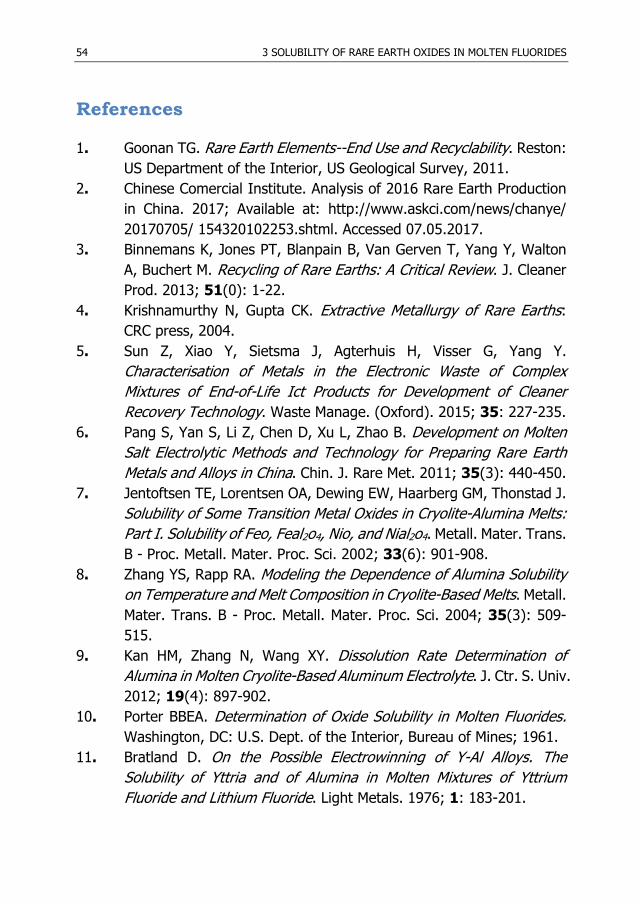
54 3 SOLUBILITY OF RARE EARTH OXIDES IN MOLTEN FLUORIDES
References
1. Goonan TG. Rare Earth Elements--End Use and Recyclability. Reston: US Department of the Interior, US Geological Survey, 2011.
2. Chinese Comercial Institute. Analysis of 2016 Rare Earth Production in China. 2017; Available at: http://www.askci.com/news/chanye/ 20170705/ 154320102253.shtml. Accessed 07.05.2017.
3. Binnemans K, Jones PT, Blanpain B, Van Gerven T, Yang Y, Walton A, Buchert M. Recycling of Rare Earths: A Critical Review. J. Cleaner Prod. 2013; 51(0): 1-22.
4. Krishnamurthy N, Gupta CK. Extractive Metallurgy of Rare Earths: CRC press, 2004.
5. Sun Z, Xiao Y, Sietsma J, Agterhuis H, Visser G, Yang Y. Characterisation of Metals in the Electronic Waste of Complex Mixtures of End-of-Life Ict Products for Development of Cleaner Recovery Technology. Waste Manage. (Oxford). 2015; 35: 227-235.
6. Pang S, Yan S, Li Z, Chen D, Xu L, Zhao B. Development on Molten Salt Electrolytic Methods and Technology for Preparing Rare Earth Metals and Alloys in China. Chin. J. Rare Met. 2011; 35(3): 440-450.
7. Jentoftsen TE, Lorentsen OA, Dewing EW, Haarberg GM, Thonstad J. Solubility of Some Transition Metal Oxides in Cryolite-Alumina Melts: Part I. Solubility of Feo, Feal2o4, Nio, and Nial2o4. Metall. Mater. Trans. B - Proc. Metall. Mater. Proc. Sci. 2002; 33(6): 901-908.
8. Zhang YS, Rapp RA. Modeling the Dependence of Alumina Solubility on Temperature and Melt Composition in Cryolite-Based Melts. Metall. Mater. Trans. B - Proc. Metall. Mater. Proc. Sci. 2004; 35(3): 509-515.
9. Kan HM, Zhang N, Wang XY. Dissolution Rate Determination of Alumina in Molten Cryolite-Based Aluminum Electrolyte. J. Ctr. S. Univ. 2012; 19(4): 897-902.
10. Porter BBEA. Determination of Oxide Solubility in Molten Fluorides. Washington, DC: U.S. Dept. of the Interior, Bureau of Mines; 1961.
11. Bratland D. On the Possible Electrowinning of Y-Al Alloys. The Solubility of Yttria and of Alumina in Molten Mixtures of Yttrium Fluoride and Lithium Fluoride. Light Metals. 1976; 1: 183-201.

REFERENCES 55
12. Du S, Wu M, Du F, Liu Y. Solubility of Rare Earth Oxides in Alkali and Alkali-Earth Metal Fluoride Melts. Chin. Rare Earths. 1987; 8(2): 59-62.
13. Morrice E, Reddy RG. Solubility and Activity Coefficient of Y2O3 in Fluoride Melts. Paper presented at: Rare Earths, Extraction, Preparation and Applications sponsored, 1989; Las Vegas, NV.
14. Wu W, Sun J, Hai L, Gao H. Nd2O3 Solubility in Fluoride Melt. Chin. Rare Earths. 1991; 12(3): 34-37.
15. Reddy RG, Kumar SG. Solubility and Thermodynamic Properties of Y2O3 in LiF-YF3 Melts. Metall. Mater. Trans. B - Proc. Metall. Mater. Proc. Sci. 1994; 25(1): 91-96.
16. Dewing EW, Haarberg GR, Rolseth S, Ronne L, Thonstad J, Aalberg N. The Chemistry of Solutions of Ceo2 in Cryolite Melts. Metall. Mater. Trans. B - Proc. Metall. Mater. Proc. Sci. 1995; 26(1): 81-86.
17. Stefanidaki E, Photiadis GM, Kontoyannis CG, Vik AF, Ostvold T. Oxide Solubility and Raman Spectra of NdF3-LiF-KF-MgF2-Nd2O3 Melts. J. Chem. Soc., Dalton Trans. 2002; (11): 2302-2307.
18. Ambrová M, Jurišová J. Solubilities of Lanthanum Oxide in Fluoride Melts Part I. Solubility in M3alf6 (M=Li, Na, K). Thermochim. Acta. 2006; 443(1): 105-108.
19. Hu X. Study on Ionic Structure and Its Application of NdF3-LiF-Nd2O3 System Melts [Ph.D. Dissertation]. Shenyang, Northeastern University; 2008.
20. Ambrová M, Jurišová J, Danielik V, Gabčová J. On the Solubility of Lanthanum Oxide in Molten Alkali Fluorides. J. Therm. Anal. Calorim. 2008; 91(2): 569-573.
21. Pshenichny RN, Omelchuk AA. Interaction of Rare-Earth Oxides with Binary Molten Mixtures of Zirconium and Alkali Metal Fluorides. Russ. J. Inorg. Chem. 2012; 57(1): 115-119.
22. Hu X, Wang ZW, Shi ZN, Lui GM, Gao BL, Cao XZ, Luo XD, Cui JZ, Nie YG, Wang C, Chen GH, Wu YW, Ma S, Lu D, Ma C. Nd2O3 Solubility in NdF3-LiF-Nd2O3 Melts. Paper presented at: Proceedings of 2007 Non-Grid-Connected Wind Power Systems, 2007; Marietta.
23. Zhang Y. Electronegativities of Elements in Valence States and Their Applications. 2. A Scale for Strengths of Lewis Acids. Inorg. Chem. 1982; 21(11): 3889-3893.

56 3 SOLUBILITY OF RARE EARTH OXIDES IN MOLTEN FLUORIDES
24. Thoma R. Phase Diagrams of Binary and Ternary Fluoride Systems. In: Braunstein J, Mamantov G, Smith GP, eds. Advances in Molten Salt Chemistry: Springer US, 1975:275-455.
25. Perry DL. Handbook of Inorganic Compounds. (Second edition). Boca Raton, FL: CRC Press, Taylor & Francis Group, 2011.
26. Hu X. Electrical Conductivity and Nd Solubility of NdF3-LiF-Nd2O3 Melts. Charact. Miner. Met. Mater. 2007: 79-82.
27. Hu X, Wang Z, Gao B, Shi Z. Study on the Electrical Conductivity of NdF3-LiF-Nd2O3 System Melts Determined by Cvcc Technique. J. NE Univ.: Nat. Sci. 2008; 29(9): 1294-1297.

4
Semiempirical Model for the
Solubility of Rare Earth Oxides in
Molten Fluorides
Abstract
he importance of recycling and producing rare earth materials has been highlighted by the critical raw materials study in the European Union.
Oxide-fluoride electrolysis is one of the dominant technologies to produce rare earth metals or alloys. The solubility of rare earth oxides is one of the critical issues during this process. In this research, a model is developed to predict the solubility of rare earth oxides in molten fluorides, based on the systematic analysis of different influential factors and fundamental understanding of the dissolution reactions. The average relative deviation of the model from the experimental data extracted from the literature is 8 % for Nd2O3 and 7 % for Y2O3, respectively, which is well within the experimental uncertainty. The fitting parameters can indicate the influence
† This Chapter is based on the paper: Guo X, Sun Z, Sietsma J, Yang Y. Semiempirical Model for the Solubility of Rare Earth Oxides in Molten Fluorides. Ind. Eng. Chem. Res. 2016; 55(16): 4773-4781.
T

58 4 SEMIEMPIRICAL MODEL FOR THE SOLUBILITY OF RARE EARTH OXIDES
of different composition quantitatively. It is also found that the solubility is correlated with the ion charge density of the cations in the molten salts.
4.1 Introduction
are earth metals (REMs) and alloys have been widely applied to state-of-the-art appliances including magnets, catalysts, batteries and
phosphors, because of their unique physical and chemical properties. In the last several decades, a dramatic increase in demand for these materials was realized by the rapid development of electronics and related industries. According to the US Geological Survey report from 2011, the production of REMs grew rapidly by 5 % per year on average from 1990 through 2007 and kept increasing even after the 2008 global financial crisis 1, which is a clear indication of the importance of REMs. In the EU, the recycling and production of rare earth materials have recently been promoted by local materials scarcity and potential supply risk. The Ad Hoc working group representing the European commission released a report about EU critical raw materials first in 2010, then 2013, and later in 2017, in which REMs are considered of top criticality 2-4. On the market, the largest amount of REMs is commercially produced by electrolytic methods, which are broadly categorized into chloride and fluoride electrolysis 5. Due to the drawbacks of a chloride cell at high temperature, such as the high volatility of chlorides, large solubility of REMs in the electrolytes, and corrosion of cell wall materials, oxide-fluoride electrolysis is nowadays frequently used and tends to dominate REM production 6. Fluoride cells, so far, have been industrialized for the production of light lanthanides, i.e. La, Ce, Pr, and Nd, and some rare earth alloys, such as Dy-Fe, Gd-Fe, Ho-Fe and Pr-Nd-Dy 7. In the process, the production of REM includes two steps: the dissolution of rare earth oxide (REOs) in a mixture of molten fluorides and electrowinning of REM at the cathode. The solubility of REOs in fluorides and in-depth understanding of the dissolution behavior are two critical aspects, of both fundamental and engineering importance, for the design of electrolyte composition and smooth process operation 5. However, research is scarce on these issues and in industrial production the addition of REO into a fluoride electrolyte still has to mostly rely on experience 7.
R

4.2 SOLUBILITY OF REOS IN MOLTEN FLUORIDES 59
Small fluctuations in the bath conditions (e.g. temperature, electrolyte composition), can sometimes significantly influence the production rate, since the REO concentration in the melts cannot be monitored and controlled on-line 8. If the REO concentration falls below a certain limit, an anode effect may be triggered, while too much undissolved REO may settle down and form a sludge at the bottom of the electrolytic cell, deteriorating the quality of the reduced metal product. In the literature, only limited research on solubility has been reported, as described in Chapter 3. One encounters difficulties to reach a consistent conclusion when the salt composition varies, or the oxides are changed. Adequate prediction of the solubility of REOs in molten fluorides is limited by the reliability of experimental measurements and understanding of the solubility behavior against the nature of fluorides. Improved understanding of the relationship between REO solubility and different factors of the fluoride melts is of considerable importance. This chapter presents a systematic evaluation of the REO solubility in fluoride electrolytes, aiming to identify possible relationships among REO solubility, temperature, and salt composition. On the basis of thermodynamics analysis, a semi-empirical model is developed to predict the solubility of REO in molten fluorides.
4.2 Solubility of REOs in molten fluorides
olubility is a physicochemical property describing a chemical substance (solute) dissolving in a solid, liquid, or gaseous solvent to form a
saturated solution. Under such conditions, the dissolution reaches an equilibrium state, and the solubility of a solute follows thermodynamic laws. As described in the previous chapter, pioneering research on REO solubility was done by Porter (1961) 9. A procedure was developed to measure the oxide content of molten fluoride systems. In this research, the focus was on CeO2 and La2O3 in a corresponding rare earth fluoride (REF)-BaF2-LiF system. In the late 1970s, Bratland and his colleagues 10 found that the solubility of Y2O3 increases with increasing ratio between YF3 and LiF in the mixtures and lithium fluoride possibly act as an inert diluent. Meanwhile, a significant effect of cation species on the solubility was also noticed by Bratland (1976) 10. For
S
60 4 SEMIEMPIRICAL MODEL FOR THE SOLUBILITY OF RARE EARTH OXIDES
instance, 50YF3-50NaF (molar ratio) has much lower Y2O3 solubility than 50YF3-50LiF. Increasing REF concentration has been observed to increase REO solubility in both binary and ternary fluoride salt systems. This was later confirmed by Morrice et al. (1989) 11 for Y2O3 and Du et al. (1987) 12 for Nd2O3. The chemical interaction between REO and lithium fluoride was found to be rather weak and LiF mainly functions as an additive to lower the melting point and improve the conductivity of the melt. However, the solubility of Nd2O3 was found to be slightly changed by the addition of MgF2 into NdF3-LiF melts 13. Moreover, the solubility of REOs in alkali metal fluoride (AF)-ZrF4 binary molten salts was found to decrease with increasing the Ln3+ ion radii ( Ho La3 3 3Smr r r+ + +< < ) and with increasing the alkali metal cation radii
( Li Na Kr r r+ + +< < ) 14. Their conclusion is consistent with the observations by
Bratland (1976) 10. In the same period, researchers have been making efforts to study the interaction between REOs and fluorides to reveal the dissolution mechanisms. The work done by Stefanidaki et al. (2002) 13 and Hu (2008) 15 using Raman spectroscopy suggests that the dissolution mechanisms follow the reactions ( ) ( )1
2 3 3Nd O NdF 3 F 3NdOF -1 yyy −−+ + − (4.1)
where y must be less than 5 due to the limitation imposed by the maximum co-ordination number of six for the Nd3+ cation. Reaction (4.1) shows that LiF is only a F- donor. In addition, according to Raman spectroscopy investigation 13, a small decrease in the intensities of the reduced anisotropic scattering relative to the isotropic scattering was observed with the dissolution of Nd2O3. This is due to diminishing dipole-induced-dipole (DID) interactions between neighboring Nd3+ cations, which was observed in liquid NdF3-LiF, by the oxygen anions. This decrease confirms the presence of the neodymium oxyfluoride complexes. It is evident that the dissolution of REOs is a process in which the REO crystal dissociates via the interaction with molten salts. Therefore, it is possible to predict more precisely the solubility of REOs if the understanding of the effects and behavior of fluoride salts during the REO dissolution is improved.

4.2 SOLUBILITY OF REOS IN MOLTEN FLUORIDES 61
Similarly, the formation of oxyfluoride complexes in the melt is critical for other REOs to ensure the process of dissolution. When REF is present in the fluoride melt, the solubility is influenced by the stability of 3-RF6 octahedra, which is not only related to the REM type, but also influenced by other surrounding metal ions. This means that the more stable the 3-RF6 octahedron is, the higher the possibility to form RE-O-F complexes associated with dissolution of REOs 13,16. This fact gives direct evidence that the solubility of REOs is a complex chemical feature. Appendix I of this thesis gives an extensive summary of the major previous studies on solubility of REOs in molten fluorides. The systems investigated include (1) unary, binary, and ternary melts, (2) melts with and without REF, (3) alkali metal salt-based and alkali earth metal salt-based systems, and (4) melts containing ZrF4 for nuclear fuel carriers. In each system, a range of factors were studied, such as temperature and salt composition. It can be noticed that the most frequently investigated REOs are Y2O3, Nd2O3 and La2O3 in LiF-based molten fluorides. LiF is a rather stable compound with lower melting point than other AFs and it is more difficult to decompose during electrolysis. The features of LiF determine the physicochemical properties of the binary or ternary molten salts and can subsequently influence the solubility of REOs together with REF 10,13. Generally speaking, the REO solubility in fluoride melts is relatively low. More than 60 % of the reported solubilities were found to be lower than 1 mol. %, and more than 90 % is under 2 mol. %. Some special cases that should be mentioned are the solubility in melts containing AlF3. For example, the solubility of La2O3 in NaF-AlF3 melt is over 10 mol.% at 1250 K. It is likely that the solubility of La2O3 is enhanced by the following reaction, which is thermodynamically favorable in the forward direction at the experimental condition: 2 3 3 3 2 3La O AlF LaF Al O2 2+ + (4.2) In fact, reaction (4.2) turns the 3-component-system to a (La2O3-)Al2O3-NaF-LaF3-AlF3 system, in which the interactions between components become extraordinarily complicated. There may be La-O-F, Al-O-F, Na-O-F, Na-Al-O-F, and even La-Al-O-F, Na-La-O-F complexes co-existing in the melt. The

62 4 SEMIEMPIRICAL MODEL FOR THE SOLUBILITY OF RARE EARTH OXIDES
solubility of Al2O3 in cryolite is in the range from a few mole percent to higher than 10 mol. % at 1123 ~ 1323 K 17. As long as reaction (4.2) moves forward and Al2O3 is not saturated in the melt, La2O3 can continue to dissolve into the melt. Therefore, it is easy to infer that the solubility of La2O3 in NaF-AlF3 system will be much higher than in other fluoride systems in which only reaction (4.1) occurs. In this case, the dissolution of REOs in reactive salts follows significantly different mechanisms. These solubility data are excluded when developing the model.
4.3 Model for REO solubility in molten fluorides
4.3.1 Influencing factors in REO solubility
n previous research 18,19, the effects of different factors, including temperature and fluoride salt composition, on the REO solubility have
been briefly discussed. It was found that the solubility increases with temperature and a linear relationship exists between the logarithm of the solubility and the reciprocal of the absolute temperature 19. Chapter 3 gives the temperature dependence of the REO solubility in a variety of fluoride salts. It can be found that CeO2 in NaF-AlF3, Y2O3 in YF3-NaF and La2O3 in LiF-NaF-KF exhibit the strongest temperature dependence, while the dependence is less pronounced for La2O3 in KF-ZrF4, Nd2O3 in NdF3-LiF and La2O3 in KF-AlF3 salts. Meanwhile, the slopes of the lines of the same REO differ in diverse melts. The salt composition clearly influences not only the solubility values but also the gradient of the solubility changing with temperature. Generally, the composition of the fluoride melt used to dissolve REOs depends on its application, varying from REM production to nuclear engineering. It may contain REF, AF, alkali earth metal fluoride (AEF), and sometimes other fluorides. The corresponding content of different salts in the molten fluoride further determine the physicochemical and thermodynamics properties, e.g., the melting point, viscosity, electrical conductivity of the melt as well as the solubility of REOs.
I

4.3 MODEL FOR REO SOLUBILITY IN MOLTEN FLUORIDES 63
The REO solubility increases with increasing REF content in the fluoride melts as discussed in chapter 3. Contributions from non-RE salts should be insignificant to the REO dissolution (Equation (4.1)), except in the case of direct chemical reactions between the REOs and salts in the melt (Equation (4.2)). In the current research, only the dissolution mechanisms following reaction (4.1) are considered. In this case, the presence of RE-O-F complex is directly associated with REO solubility. The complex can have different forms. For example, for Nd2O3 dissolution in NdF3-LiF salts, the complex can be monomers as 3-NdOF4 , 4-NdOF5 and dimers as 4-Nd OF2 8 and 6-Nd OF2 10 13,15. Comparing the existing solubility data, this is in line with the favorable influence of REF content to increase the solubility of REOs. However, the melting points of REFs are rather high 20. The current electrolytic cell operation requirements cannot be fulfilled using only REF salts as an electrolyte 8 (operation temperature below 1400 K). AF is a common additive to ensure REO electrolysis because of their low melting points and relatively high electrochemical and thermodynamic stability. In the case of LiF, the eutectic points are 19 ~ 27 mol. % REF (around 70 wt. %) at around 1000 K 21 as given in Figure 4.1, which shows the potential of decreasing the operational temperatures. At the same time, other physicochemical properties, e.g., conductivity, viscosity, and surface tension, also need to be considered in the selection of proper fluoride salts for REO electrolysis. Research showed that the addition of LiF could increase the electrical conductivity of NdF3-LiF binary system due to the lower resistance of movement and higher mobility of Li+ than that of Nd3+ 15. AEF is sometimes used in the melts in order to further lower the melting points of the electrolyte, and in most cases the evaporation of AF as well as the melt viscosity can be minimized 5.
4.3.2 Model for REO solubility
n order to generalize the analyses, the dissolution of REOs into fluoride melts can be simplified as the following reaction REO(solid) REO(dissolved) (4.3) I

64 4 SEMIEMPIRICAL MODEL FOR THE SOLUBILITY OF RARE EARTH OXIDES
Figure 4.1 Melting points of REF and eutectic points of REF-AF
binary systems with the difference given in K
At equilibrium, the standard Gibbs energy change of the dissolution reaction
0sol REOGΔ equals 0
sol REO REOln lnG RT K RT aΔ = − = − (4.4) If a hypothetical undercooled liquid REO at the temperature of the experiment (T ) is used as a standard state for the activity REOa , the standard Gibbs free energy change for REO dissolution, 0
sol REOGΔ , can be considered as the standard Gibbs energy change of the melting of REO into the fluoride salt at m, REOT T< . This implies 0 0 0 0
sol REO f REO(l) f REO(s) fus REOG G G GΔ = Δ − Δ = Δ (4.5) where 0
f REO(l)GΔ and 0f REO(s)GΔ are the standard Gibbs energy of REO at the
liquid and solid state, respectively, and 0fus REOGΔ the standard Gibbs energy
change during fusion.
YF 3La
F 3CeF 3
PrF 3NdF 3
SmF 3
GdF 3DyF 3
HoF 3800
1000
1200
1400
1600
1800
2000
453
723
682
649
639
608
531
454
433
Melting point of REF Eutectic point of LiF-REF
Tem
pera
ture
(K)

4.3 MODEL FOR REO SOLUBILITY IN MOLTEN FLUORIDES 65
In addition, REO REO REOa sγ= (4.6) Combining the above equations, the relationship between REOs and T can be represented as fus REO
REOREO
01 exp( )Gs
RTγΔ
= − (4.7) The expression describes the thermodynamics of the dissolution of REO in a molten fluoride salt. For a solid REO molecule to dissolve into the melt, it follows the following principal steps 14,22-24: 1) Dissociation of REO long-range ordered crystal lattice or structure (from
solid to metastable state). This process can be considered as the fusion of REO and is mainly determined by the physicochemical properties of the oxide.
2) REO forms a new short-range ordered lattice (from metastable state to
liquid). It is a process in which REO interacts with the molten fluoride salt and the association of REO with the melt matrix is rather important. In this process, temperature and the melt properties, including composition of the salt and its liquid structure, will be critical to determine the extent of REO dissolution in the melt.
According to the symmetric formalism for multi-component regular solutions25, the activity coefficient for each end-member k can be calculated as: -1
1ln n n
k i j iji j i
RT q q Wγ= >
= − (4.8) where 1i iq x= − for i k= and i iq x= − for i k≠ , ix is the mole percentage of component i , ijW are binary regular interaction parameters, which can be simple functions of temperature and pressure, according to ij ij ij ijW a b T c P= + + (4.9)

66 4 SEMIEMPIRICAL MODEL FOR THE SOLUBILITY OF RARE EARTH OXIDES
where ija , ijb and ijc are constants. Since the systems concerned in this paper are under constant pressure, the third term in the above equation can be merged with other constant terms
( )ij ijij ija c PW b T+= + (4.10) As i jq q , ij ija c P+ , and ijb are independent of temperature, the activity coefficient can be simplified as
REO
* *ln lnA BRT
γ = − − (4.11) with *A and *B being temperature independent. By substituting Equation (4.11) into the thermodynamic expression of REO solubility (Equation (4.7)), it becomes
fus REO fus REOREO REO
0 0 ** ( )1ln ln lnG G As BR T RT
γ Δ Δ −= − − ⋅ = − (4.12)
Assuming 0
sol REOG a bTΔ = − (4.13) where a and b are temperature-independent parameters, the solubility expression changes into
REO
* ** *( ) ( )ln ln lna bT A b a As B BRT R RT
− − − = − = + −
(4.14) It can be found that the REO solubility expression is in line with the experimental results, i.e., a linear relationship between REOln s and 1
T .
Based on Equation (4.14), a model for REO solubility in REF-containing fluoride salts can be proposed and the expression can be simplified as
REOln ln As xRT
= − (4.15) or
REO exp As xRT
= ⋅ −
(4.16)

4.4 RESULTS AND DISCUSSION 67
where the temperature-independent parameters are defined as * exp bx B
R = ⋅
and *A a A= − .
For multicomponent systems, x is non-linearly correlated with the concentrations of different components ix in the melt and can be expressed as 1 1 2 2
2 2 21 11 1 12 2 22 2 3 3 33 3 ......x c x c x c x x c x c x c x c x= + + + + + + + (4.17) where ic and ijc are the correlation coefficients indicating the dependence
on different terms, e.g. 1x , 1 2x x , …, and subscripts, 1, 2, 3, …, denote different fluoride components. For a specific system, not all terms are necessarily included in the model, since in most cases, only some of them are significant for the solubility. Model parameters, i.e. A , ic , and ijc , can be obtained by fitting the experimental data to Equation (4.15) using a software application for data analysis and scientific graphing, OriginPro 9.0 26. The best result was obtained by comparing all possibilities (combinations of different term(s) in the model) using Akaike’s Information Criterion (AIC) Test. This is a criterion for model selection and estimates the relative quality of different models for a given set of data. Take a binary melt as an example. There are 31 different combinations, i.e., 1 1c x , ( 1 1c x , 211 1c x ), ( 1 1c x , 2 2c x )…etc. Among these possibilities, the one that fits the experimental results best was chosen using the AIC Test. The fitting parameters obtained, thereafter, can be used to estimate the solubility with minimized experimental efforts and at conditions with experiment difficulties.
4.4 Results and discussion
4.4.1 Nd2O3 solubility in NdF3-LiF(-MgF2/CaF2) melts
eodymium is one of the most important REMs with its main application in permanent magnets, which still has to be prepared mostly with N

68 4 SEMIEMPIRICAL MODEL FOR THE SOLUBILITY OF RARE EARTH OXIDES
powder metallurgy using pure neodymium metal. At the same time, this metal, nowadays, is mainly produced by electrolysis in fluoride molten salts. The salt system is usually REF-LiF-based, and AEF is one of the important additives for optimizing the melt properties to fulfil the electrolysis conditions at different practices 13,27,28. The Nd2O3 solubility in NdF3-LiF-(MgF2/CaF2) systems is therefore considered using the current model. Following the procedures described in section 4.3, the parameters in the solubility model can be obtained by comprehensively integrating the experimental solubility data (Table S1) into Equations (4.15) and (4.17), and the results are given in Table 4.1. It is necessary to mention that the parameters are valid for fluoride melts with 5 ~ 50 mol.% of NdF3, 0 ~ 11 mol.% of MgF2, and 0 ~ 19 mol.% of CaF2 at temperature 1023 ~ 1423 K. The effects of different fluoride salts, which are reflected by the correlation coefficients, are found to be varying. A positive coefficient value means that the term in Equation (4.17) has a positive effect on the Nd2O3 solubility, i.e.
NdF3x , 2LiF MgFx x , and
2CaFx in this case, while a negative value implies that
increasing the value of the term will decrease the oxide solubility, i.e. LiFx , and
2MgFx in this case. Terms that are missing, e.g., 3NdF LiFx x for the NdF3-LiF-
(MgF2/CaF2) systems, have no or insignificant effect on the oxide solubility.
Table 4.1 Model parameters for Nd2O3 solubility in NdF3-LiF-(MgF2/CaF2) systems
Value# Standard Error
A (kJ/mol) 40 3
1c * 1.1 0.3
2c * -0.12 0.02
3c * -4 2
23c * 5 2
4c * 1.1 0.2 * 1 - NdF3, 2 - LiF, 3 - MgF2, 4 - CaF2
# Values valid for 3 systems, i.e., NdF3-LiF, NdF3-LiF-MgF2, NdF3-LiF-CaF2 with 5 ~ 50 mol.% of NdF3, 0 ~ 11 mol.% of MgF2, and 0 ~ 19 mol.% of CaF2 at temperature 1023 ~ 1423 K

4.4 RESULTS AND DISCUSSION 69
The predicted values are compared with experimental data to verify the accuracy of the model. Figure 4.2 shows the relative deviation of this model from each datum for Nd2O3 solubility in diverse melt systems (purple dots on the right portion). The median value of the errors (0.041 %) is close to zero, and most of the values lie within one standard deviation of the mean (indicated by the error bar on the left portion). That is, the positive and negative relative errors are randomly and evenly distributed for the current model. This confirms that there is no obvious system error, and the model can truly reflect the influences of different factors.
Figure 4.2 Relative error between the experimental data and the data calculated with the current model for Nd2O3 solubility
The absolute values of the relative error shown in Figure 4.2 are calculated and drawn in Figure 4.3 with respect to the Nd2O3 solubility. The average value is 8 %, which is well within experimental uncertainty (13 % on average 13). This confirms the high accuracy of this solubility model. One may notice that the error is large at low solubility. The main reason is the large relative
0.041
-40
-30
-20
-10
0
10
20
30
40
Rel
ativ
e er
ror (
%)
Nd2O3
%

70 4 SEMIEMPIRICAL MODEL FOR THE SOLUBILITY OF RARE EARTH OXIDES
experimental error introduced when determining low oxide concentration in melts.
Figure 4.3 Absolute values of relative error for Nd2O3 solubility model
Figure 4.4 shows the model results for NdF3-LiF system without additives. The experiment data are included using open circles. Good agreement between the predicted values and the experimental data can be observed. The solubility increases with the increase of both temperature and NdF3 content. As indicated previously, the contribution from LiF is to be a donor of F- and to decrease the operational temperature for electrolysis. This can be further notified by comparing the slopes of different solubility profiles of the model. When the NdF3 content is relatively low, e.g., 15NdF3-85LiF, the profile is rather steep, indicating that the temperature increase has significant effect on the oxide solubility. Even reaching the operation temperature of industrial cells (around 1350 K 7), the solubility is still too low to be feasible for efficient electrolysis. However, the increase of NdF3 in the melts can increase their melting temperatures and other physicochemical properties, e.g., viscosity and conductivity, will be further influenced. In
0.0 0.5 1.0 1.5 2.0 2.5
0
10
20
30R
elat
ive
erro
r (%
)
Nd2O3 solubility (mol. %)
Mean 8
+1 SD 17
-1 SD -1

4.4 RESULTS AND DISCUSSION 71
practice, it is required to consider both the solubility and other melt properties in order to ensure efficient electrolysis conditions.
Figure 4.4 Nd2O3 solubility in melts with different NdF3 concentration and at different temperatures
Generally, LiF functions as a dilution of the melt and the increase of LiF content is observed to decrease the REO solubility. However, the effects of additives to LiF-REF systems are more complex, not only because the additives may decrease the melting point of the melt, but also interactions between the added salt and LiF or NdF3 may take place. Since the solubility of REOs is mainly related to their reaction with REF via Equation (4.1), the effect of other metal ions on the interaction or bonding between RE ions (RE3+) and fluoride ions is possibly influencing the extent of the dissolution reaction (Equation (4.1)). The solubility is found to be related to the stability of the 3-REF6 octahedral complex, which is noticed to be associated with the charge density (σ) of different cations in the melt 29,30. The higher the charge density, the more stable the 3-MF6 (M = metal) octahedra and the greater the
0.0 0.5 1.0 1.5 2.0
1000
1100
1200
1300
1400
1500Te
mpe
ratu
re (K
)
Nd2O3 solubility (mol. %)
15NdF3-85LiF (model) 23NdF3-77LiF (model) 30NdF3-70LiF (model) 42NdF3-58LiF (model) 50NdF3-50LiF (model) 60NdF3-40LiF (model) Experimental Data (Table A1)

72 4 SEMIEMPIRICAL MODEL FOR THE SOLUBILITY OF RARE EARTH OXIDES
tendency towards the formation of an M-O-F complex anion. It is also believed that the metal cations are associated with the complex anion by ionic or covalent bonds to form long-range ordered structure. Figure 4.5 shows the ionic charge density values of some metal ions. The charge density was calculated using 2Zrσ = (4.18) where Z is the charge number of an ion, and r is the effective ionic radii taken from the reference 31. The radii are a function of anion and cation coordination and electronic spin state. All ions considered here only have an electronic spin state. As discussed previously, 3-MF6 octahedral complex is important to the solubility. Hence, the radii with coordination number of 6 were taken in our calculations.
Figure 4.5 Ionic charge density of different metal ions in the fluoride melts
Li(I)
Na(I)
K(I)Mg(I
I)Ca(I
I)Ba(I
I)Zr(IV
)Y(III
)La
(III)
Ce(III)
Ce(IV)
Nd(III)
0.0
2.0
4.0
6.0
8.0IA IIA IVB Lanthanide
Ioni
c ch
arge
den
sity
, Z /
r2 (Å-2)

4.4 RESULTS AND DISCUSSION 73
Considering the ionic charge density, Li+ has a weaker charge effect on F- than RE3+ and therefore Li+ shows a negative effect on the dissolution reaction. When a certain additive, e.g., Ca2+, is added to partially replace the Li+ in the fluoride melts, the REO solubility can be increased because the ionic charge density of Ca2+ is larger than that of Li+. This is in line with experimental observations for the effect of CaF2 addition on the solubility data (Figure 4.6). However, more fundamental information on the melt structures is still required to acquire more quantitative understanding. For the model, the correlation coefficient is found to be positive, showing consistency with experimental observations (Table 4.1). As given in Figure 4.6, the increase of solubility with CaF2 addition is valid for both low and relatively high NdF3 contents.
Figure 4.6 Relationship between Nd2O3 solubility and CaF2 concentration at 1303 K
The effects of MgF2 are however different from CaF2 and are more complex than those of CaF2. Because the ionic charge density of Mg2+ is higher than that of Nd3+. Figure 4.7 shows the model results as well as the comparison
14 16 18 200.0
0.2
0.4
0.6
0.8
1.0
Nd 2
O3 s
olub
ility
(mol
. %)
CaF2 concentration (mol. %)
5NdF3-LiF-CaF2 (model) 10NdF3-LiF-CaF2 (model) 20NdF3-LiF-CaF2 (model) Experimental Data (Table A1)
at 1303 K

74 4 SEMIEMPIRICAL MODEL FOR THE SOLUBILITY OF RARE EARTH OXIDES
with experimental data. It can be noticed that the addition of MgF2 generally has a negative effect on the oxide solubility with a negative coefficient value. On the one hand, the replacement of LiF in the melt may increase the REO solubility (positive effect). This effect can be dominant at low REF content or becomes pronounced when LiF content increases. On the other hand, it is noticed that the mutual solubility between the two salts is rather high according to the phase diagram of MgF2-LiF 21. There is a possibility of forming Mg-Li-F clusters/complexes in the melt and in this case the addition of MgF2 replacing LiF may introduce a stronger charge effect on F- than RE3+ and the stability of 3-REF6 octahedra can be disturbed. This is subsequently bringing a negative effect on the solubility (Equation (4.1)).
Figure 4.7 Relationship between Nd2O3 solubility and MgF2 concentration at 1133 K
4.4.2 Y2O3 solubility in YF3-LiF/NaF melts
he solubility measurements for Y2O3 were mainly conducted in YF3-LiF/NaF systems 10,32. It was observed experimentally that its solubility
0 2 4 6 8 10 12 140.0
0.1
0.2
0.3
0.4
Nd 2
O3 s
olub
ility
(mol
. %)
MgF2 concentration (mol. %)
15NdF3-LiF-MgF2 (model) 30NdF3-LiF-MgF2 (model) Experimental Data (Table A1)
at 1133 K
T

4.4 RESULTS AND DISCUSSION 75
in YF3-based fluorides is usually higher than that of Nd2O3 in NdF3-based melts. This may be attributed to their difference in ionic charge density. That is, Y3+ has a higher charge density than Nd3+, resulting in a more stable long-range structure. However, this is not necessarily always the case since solubility is also determined by other physicochemical properties of the melt. Figure 4.8 compares two sets of solubility data for Y2O3 in YF3-LiF melts from different investigations 10,32. It can be noticed that the solubility values from Reddy et al. (1994) 32 are significantly higher than those from Bratland (1976) 10.
Figure 4.8 Y2O3 solubility in melts with different YF3 concentration and at different temperatures
The discrepancy between the two studies is probably due to the different techniques used for solubility measurement. Reddy et al. (1994) 32 determined Y2O3 solubility by chemical analysis of Y, Li, F, and O in representative samples taken during experiments, while Bratland (1976) 10 visually determined the saturation temperature of the melt with a known concentration of Y2O3 by repeatedly slow heating and cooling the melt. The
0.0 0.5 1.0 1.5 2.0 2.5 3.0 3.5
1000
1100
1200
1300
1400
1500
Tem
pera
ture
(K)
Y2O3 solubility (mol. %)
25YF3-75LiF (model) 50YF3-50LiF (model) Experimental data (Ref. 32) Experimental data (Ref. 10)

76 4 SEMIEMPIRICAL MODEL FOR THE SOLUBILITY OF RARE EARTH OXIDES
latter is based on visual observation and its error should be much higher than the chemical analysis used by Reddy et al. (1994) 32. In addition, the heating or cooling rate must have been well chosen to make sure the equilibria (quasi-equilibria) were reached. Otherwise, the measured solubility would be lower than the real value. The system was quite sensitive to the air that was occasionally allowed into the gas-tight system. In case of any leakage, the observed saturation temperature increases as the oxide concentration increases because of H2O absorption. This could also result in an unreliable measured solubility, which is probably lower than a real value. Consequently, the data set from Bratland (1976) 10 is not covered when developing the solubility model for Y2O3 to make sure the validity of the model for predicting unknown solubilities. The parameters of the model developed based on the data from Reddy et al. (1994) 32 are listed in Table 4.2. The effect of YF3 is positive, while
3YF LiFx x shows a slightly negative effect on the solubility. Table 4.2 Equation parameters for Y2O3 solubility in YF3-LiF system
(fitted with data from Reddy et al. (1994) 32)
Value# Standard Error
A (kJ/mol) 45 3
1c * 4 1
12c * -2.5 0.6 * 1 - YF3, 2 – LiF # Values valid for YF3-LiF with 20 ~ 50 mol. % of YF3 at 998 ~ 1273 K The predicted data using parameters in Table 4.2 is compared with experimental results 32 in YF3-LiF melts. Figure 4.9 shows the relative deviation of the calculated solubility from experimental data (purple dots on the right portion). The median value is about 1.0 % and therefore slightly deviates from zero. The relative errors are rather evenly distributed on both

4.4 RESULTS AND DISCUSSION 77
sides as shown in Figure 4.9. It can be concluded that the model does not introduce a systematic error when predicting the Y2O3 solubility.
Figure 4.9 Relative error between the experimental data and the data calculated with the current model for Y2O3 solubility
The absolute values of the relative errors are shown in Figure 4.10, with an average of 7 %. However, the experimental accuracy was not mentioned in the paper 32. Considering that a similar technique was used in the reference 13, it is reasonable to assume that the experimental uncertainty is around 13% on average. This suggests that the model can reproduce the solubility used for parameterization within the experimental accuracy. Similarly, the relative error is large at low concentrations due to the large relative experimental error introduced when the oxygen concentration is low. The absolute solubility measured by Bratland (1976) 10 is probably lower than the real values due to the technique used. However, the influence of different factors suggested by the results is still meaningful as the system errors did not change the relative values. In Bratland’s work 10, the effect of different
1.0
-30
-20
-10
0
10
20
30
Rel
ativ
e er
ror (
%)
Y2O3
%

78 4 SEMIEMPIRICAL MODEL FOR THE SOLUBILITY OF RARE EARTH OXIDES
Figure 4.10 Absolute values of relative errors for Y2O3 solubility model
AFs on the Y2O3 solubility was investigated, as given in Figure 4.11. The solubility of Y2O3 in YF3-LiF is apparently higher than that in YF3-NaF and the values can be nearly double, especially at higher temperatures. This phenomenon is directly related to the physicochemical features of the fluoride melts and can be qualitatively explained by the ionic charge density difference of different metal ions. That is, the ionic charge density of Li+ is higher than that of Na+ (Figure 4.5). The solubility sequence for different fluoride salts is also found to follow the change of weighted cationic charge density, which is
3 3 3 350YF -50LiF 50YF -50NaF 25YF -75LiF 25YF -75NaFσ σ σ σ> > > . However, it
may become complex when the ionic charge density of the added cation salt is higher than that of the rare earth ion in the fluoride melt, e.g., Mg2+.
4.4.3 Comparison of the solubility of Nd2O3 and Y2O3
Figure 4.12 compares the solubility of Nd2O3 and Y2O3 into the corresponding REF-based fluoride salts. It is clear that the solubility of
0.0 0.5 1.0 1.5 2.0 2.5
0
10
20
30
Rel
ativ
e er
ror (
%)
Y2O3 solubility (mol. %)
Mean 7
-1 SD 0
+1 SD 14
F

4.4 RESULTS AND DISCUSSION 79
Figure 4.11 Comparison of Y2O3 solubility between YF3-LiF and YF3-NaF system (reproduced with data from reference 10)
Figure 4.12 Comparison of Nd2O3 and Y2O3 solubility in REF-LiF system
0.0 0.5 1.01000
1100
1200
1300
1400
Tem
pera
ture
(K)
Y2O3 solubility (mol. %)
25YF3-75LiF 50YF3-50LiF 25YF3-75NaF 50YF3-50NaF
0.0 1.0 2.0 3.0 4.0900
1000
1100
1200
1300
1400
1500
Tem
pera
ture
(K)
REO solubility (mol. %)
Y2O3 in 50YF3-50LiF (model) Nd2O3 in 50NdF3-50LiF (model) Experimental Data (Table A1)

80 4 SEMIEMPIRICAL MODEL FOR THE SOLUBILITY OF RARE EARTH OXIDES
Y2O3 is higher than that of Nd2O3, and the solubility of Y2O3 is more sensitive to the temperature compared with that of Nd2O3. This is consistent with the model parameters, showing that A is larger for Y2O3. This is also in line with the charge density effect that Y3+ is attributed to higher RE-O-F complex stability than Nd3+. Furthermore, other physicochemical properties, for instance the viscosity, conductivity, and possible association among different ions to form different types of complexes, can also be important in determining the REO solubility. However, this field still requires significant fundamental exploration and understanding of the chemistry and structural features of the melt can be extremely critical.
4.5 Conclusions
model based on the thermodynamics analysis is developed in this study to predict the solubility of REOs in molten fluorides. The model
parameters for Nd2O3 and Y2O3 solubility are obtained by fitting experimental data extracted from the literature to the present model. The fitting parameters, furthermore, reveal the influence of different components on the solubility quantitatively. Additionally, the ionic charge density is used to explain the effects qualitatively on a theoretical basis. The conclusions can be formulated as follows. 1) The accuracy of the solubilities predicted by the model is shown to be on
average 8 % for Nd2O3 and 7 % for Y2O3, which are well within the experimental uncertainty. With these parameters, the prediction of Nd2O3 and Y2O3 solubility in certain fluoride melts at valid temperature ranges will be possible with given temperature and salt composition.
2) The model parameters shows that for Nd2O3 solubility, NdF3x ,
2LiF MgFx x , and
2CaFx have positive effects, while LiFx and 2MgFx have negative effects.
Meanwhile, the effect of YF3 is quite distinctly positive, and 3YF LiFx x shows
a negative effect on Y2O3 solubility. The value of A for Y2O3 solubility is larger than that for Nd2O3, indicating that Y2O3 solubility is more sensitive to temperature than that of Nd2O3.
A

4.5 CONCLUSIONS 81
3) The effects of different components on the solubility are found to be semi- quantitatively associated with the charge density of corresponding cations. The higher the charge density, the more positive the effect on the solubility is, and vice versa. More specifically, addition of CaF2 can increase the solubility of Nd2O3 in the NdF3-LiF binary system because the charge density of Ca2+ is larger than that of Li+. Similarly, the Y2O3 solubility in YF3-LiF is higher than that in YF3-NaF as the charge density of Li+ is higher than that of Na+. The solubility of Nd2O3 is found to be lower than that of Y2O3 in the corresponding REF-based fluoride salts due to lower charge density of Nd3+ than that of Y3+. Influence of MgF2 in NdF3-LiF-MgF2 is more complex because of the interaction between LiF and MgF2.

82 4 SEMIEMPIRICAL MODEL FOR THE SOLUBILITY OF RARE EARTH OXIDES
References
1. Goonan TG. Rare Earth Elements--End Use and Recyclability. Reston: US Department of the Interior, US Geological Survey, 2011.
2. European Commission. Critical Raw Materials for the Eu: European Commission; 2010.
3. European Commission. Report on Critical Raw Materials for the Eu: European Commission; May 2014.
4. European Commission. Commission Communication on the 2017 List of Critical Raw Materials for the Eu. Brussels: European Commission; 2017.
5. Krishnamurthy N, Gupta CK. Extractive Metallurgy of Rare Earths: CRC press, 2004.
6. De Castro JA, Rodrigues D, De Campos MF. From Neodymium Oxide to Ndfeb Alloy: An Overview on the Reduction Methods. Paper presented at: Proceedings of 23rd International Workshop on Rare Earth and Future Permanent Magnets and Their Applications REPM, 2014.
7. Pang S, Yan S, Li Z, Chen D, Xu L, Zhao B. Development on Molten Salt Electrolytic Methods and Technology for Preparing Rare Earth Metals and Alloys in China. Chin. J. Rare Met. 2011; 35(3): 440-450.
8. Zhu H. Rare Earth Metal Production by Molten Salt Electrolysis. In: Kreysa G, Ota K-i, Savinell R, eds. Encyclopedia of Applied Electrochemistry: Springer New York, 2014:1765-1772.
9. Porter BBEA. Determination of Oxide Solubility in Molten Fluorides. Washington, DC: U.S. Dept. of the Interior, Bureau of Mines; 1961.
10. Bratland D. On the Possible Electrowinning of Y-Al Alloys. The Solubility of Yttria and of Alumina in Molten Mixtures of Yttrium Fluoride and Lithium Fluoride. Light Metals. 1976; 1: 183-201.
11. Morrice E, Reddy RG. Solubility and Activity Coefficient of Y2O3 in Fluoride Melts. Paper presented at: Rare Earths, Extraction, Preparation and Applications sponsored, 1989; Las Vegas, NV.
12. Du S, Wu M, Du F, Liu Y. Solubility of Rare Earth Oxides in Alkali and Alkali-Earth Metal Fluoride Melts. Chin. Rare Earths. 1987; 8(2): 59-62.

REFERENCES 83
13. Stefanidaki E, Photiadis GM, Kontoyannis CG, Vik AF, Ostvold T. Oxide Solubility and Raman Spectra of NdF3-LiF-KF-MgF2-Nd2O3 Melts. J. Chem. Soc., Dalton Trans. 2002; (11): 2302-2307.
14. Pshenichny RN, Omelchuk AA. Interaction of Rare-Earth Oxides with Binary Molten Mixtures of Zirconium and Alkali Metal Fluorides. Russ. J. Inorg. Chem. 2012; 57(1): 115-119.
15. Hu X. Study on Ionic Structure and Its Application of NdF3-LiF-Nd2O3 System Melts [Ph.D. Dissertation]. Shenyang, Northeastern University; 2008.
16. Ambrová M, Jurišová J, Danielik V, Gabčová J. On the Solubility of Lanthanum Oxide in Molten Alkali Fluorides. J. Therm. Anal. Calorim. 2008; 91(2): 569-573.
17. Skybakmoen E, Solheim A, Sterten A. Alumina Solubility in Molten Salt Systems of Interest for Aluminum Electrolysis and Related Phase Diagram Data. Metall. Mater. Trans. B - Proc. Metall. Mater. Proc. Sci. 1997; 28(1): 81-86.
18. Guo X, Sietsma J, Yang Y. Solubility of Rare Earth Oxides in Molten Fluorides. Paper presented at: ERES2014: 1st European Rare Earth Resources Conference, 2014; Milos, Greece.
19. Guo X, Sietsma J, Yang Y. A Critical Evaluation of Solubility of Rare Earth Oxides in Molten Fluorides. In: de Lima IB, Filho WL, eds. Rare Earths Industry. Boston: Elsevier, 2016:223-234.
20. Lide DR. Crc Handbook of Chemistry and Physics. Boca Raton, Florida: CRC Press, 2005.
21. Thoma R. Phase Diagrams of Binary and Ternary Fluoride Systems. In: Braunstein J, Mamantov G, Smith GP, eds. Advances in Molten Salt Chemistry: Springer US, 1975:275-455.
22. Casey WH, Ludwig C. The Mechanism of Dissolution of Oxide Minerals. Nature. 1996; 381(6582): 506-509.
23. Veshchunov M, Hofmann P, Berdyshev A. Critical Evaluation of Uranium Oxide Dissolution by Molten Zircaloy in Different Crucible Tests. J. Nucl. Mater. 1996; 231(1): 1-19.
24. Guo X, Sun Z, Van Dyck J, Guo M, Blanpain B. In-Situ Observation on Lime Dissolution in Molten Metallurgical Slags-Kinetic Aspects. Ind. Eng. Chem. Res. 2014; 53(15): 6325-6333.
25. Powell R, Holland T. On the Formulation of Simple Mixing Models for Complex Phases. Am. Mineral. 1993; 78(11-12): 1174-1180.

84 4 SEMIEMPIRICAL MODEL FOR THE SOLUBILITY OF RARE EARTH OXIDES
26. May RA, Stevenson KJ. Software Review of Origin 8. J. Am. Chem. Soc. 2009; 131(2): 872-872.
27. Soare V, Burada M, Ostvold T, Kontoyannis C, Stefanidaki E. Study of the Mg-Nd Alloy Obtained by Electrolysis in Molten Oxifluoride Media. J. Min. Metall., B: Metall. 2003; 39(1-2): 209-221.
28. Thudum R, Srivastava A, Nandi S, Nagaraj A, Shekhar R. Molten Salt Electrolysis of Neodymium: Electrolyte Selection and Deposition Mechanism. Miner. Process. Extr. Metall. 2010; 119(2): 88-92.
29. Brown PL, Sylva RN, Ellis J. An Equation for Predicting the Formation Constants of Hydroxo-Metal Complexes. J. Chem. Soc., Dalton Trans. 1985; (4): 723-730.
30. Birdi K. Handbook of Surface and Colloid Chemistry: CRC Press, 2002. 31. Shannon RD. Revised Effective Ionic Radii and Systematic Studies of
Interatomic Distances in Halides and Chalcogenides. Acta Crystallogr. Sect. A. 1976; 32(5): 751-767.
32. Reddy RG, Kumar SG. Solubility and Thermodynamic Properties of Y2O3 in LiF-YF3 Melts. Metall. Mater. Trans. B - Proc. Metall. Mater. Proc. Sci. 1994; 25(1): 91-96.

5
Diffusion-Limited Dissolution of
Spherical Particles: A Critical
Evaluation and Applications of
Approximate Solutions‡
Abstract
he analytical and numerical description of the effective dissolution kinetics of spherical particles into a solvent is often difficult in chemical
and metallurgical engineering. The crucial first step is to identify the dissolution mechanisms, and subsequently, relevant kinetics parameters can be calculated. In this paper, three frequently used approximations, i.e., the invariant-field (Laplace), reverse-growth, and invariant-size (stationary-interface) approximations, are systematically discussed and compared with numerical simulation results. The relative errors of the dissolution curves and total dissolution time of the three approximations to the numerical simulations are calculated. The results reveal the appropriate application
‡ This Chapter is based on the paper: Guo X, Sietsma J, Yang Y, Sun Z, Guo M. Diffusion-Limited Dissolution of Spherical Particles: A Critical Evaluation and Applications of Approximate Solutions. AlChE J. 2017; 63(7): 2926-2934.
T

86 5 DIFFUSION-LIMITED DISSOLUTION OF SPHERICAL PARTICLES
ranges of the approximations for given precision levels. With further experimental validation, this research provides a methodology to properly assess dissolution kinetics and adequately estimate effective diffusion coefficients and activation energy under the experimental uncertainties.
5.1 Introduction
issolution is a process of dissolving gases, liquids or solids into a solvent and is a phenomenon that is widely occurring in the field of chemical
and metallurgical engineering, such as precipitate dissolution during the heat treatment of steels 1, drug release from solid pharmaceutical dosage forms 2, dissolution of fluxes in metallurgical processes 3. One of the most important aspects of dissolution is the kinetics, which can be identified by the rate-limiting step(s), as well as relevant kinetics parameters 4. In a stagnant fluid or solid, dissolution rate can be controlled either by the diffusion of solute atoms or molecules in the medium, or the interface reaction that transfers atoms or molecules across the phase interface 5. For diffusion-limited dissolution process, the concentration field in the fluid can be described using Fick’s second law. However, an exact analytical solution is only possible for planar particles or precipitates 6. For spherical ones, several approximate analyses have been suggested to simplify the mathematics 6. The invariant-field (IF) (Laplace), reverse-growth (RG), and invariant-size (IS) (stationary-interface) approximations are three frequently used approximate methods 6. Due to the lack of an exact analytical solution, their accuracy and application ranges have scarcely been evaluated systematically and quantitatively in the literature 6. However, when these approximations are applied to academic research, their accuracy is of the first order of importance. Otherwise, the reliability of the results (e.g., derived physiochemical parameters - diffusion coefficient) is not clear and conclusions may be misleading. With the aid of computer technology, the diffusion equations were solved numerically 5,7-12. The numerical solutions should be considered to be more accurate than analytical approximations as they take into account the effects of the moving boundary and the resulting radial convective transport, which are ignored in approximate methods 6-8. Even though the numerical simulations can produce more reliable solutions
D

5.2 APPROXIMATE SOLUTIONS FOR DISSOLUTION OF A SINGLE PARTICLE 87
proper model. An appropriate analytical approximation can be very efficient as long as the errors can be controlled at the desired levels. Confocal scanning laser microscopy (CSLM) can provide an in-situ observation of physicochemical phenomena at high temperatures. This advanced technique has been applied to studying various dissolution phenomena in metallurgical processes 13-16. In this chapter, the theory is validated with experimental results obtained with CSLM. The present research is carried out in accordance with the significance of systematic evaluation of approximate methods to validate their applicability. Three approximations, i.e., IF, RG, and IS approximations, are considered and compared with numerical simulations. This chapter presents a full picture of the accuracy of the three approximations in terms of a physicochemical parameter, k . The outcome can be served as a guideline for the applications in the scientific field. With a systematically understanding of the features of the IF, RG and IS approximations, their feasibility for dissolution kinetics is assessed with experimental data. Two examples with diverse values of the physicochemical parameter k are given. One example is taken from our previous work, studying the dissolution behavior of alumina particles in a CaO-Al2O3-SiO2 melt 15. This literature also provided numerical simulation results, which will give strong support to the present work with direct comparison with approximate solutions. The other is from the present work - the dissolution of Nd2O3 particles in LiF-24 (mol. %) CaF2.
5.2 Approximate Solutions for Dissolution Kinetics
of a Single Particle in an Infinite Medium
5.2.1 General Assumptions and Equations
o consider the general problem of the diffusion-limited dissolution of a spherical particle with initial radius, 0r , in an infinite medium, several
assumptions were made for simplifying geometrical and dissolution conditions:
T

88 5 DIFFUSION-LIMITED DISSOLUTION OF SPHERICAL PARTICLES
1) The dissolution occurs at a sharp interface between the particle and medium, and equilibrium is obtained at the interface.
2) There are no solid products formed surrounding the particle during
dissolution, i.e., the substance of the particle dissolves directly in the medium.
3) The particle consists of pure substance and is homogeneous, i.e., the
composition of the particle, PC , is considered to be constant, and is independent of the radial distance, x , from the center of the particle, and time, t .
4) The effective diffusion coefficient, D , is used to describe the complex
interdiffusion of particle atoms/molecules in the solution, i.e., a multicomponent system is treated as a quasi-binary system of the solute and medium. In the scope of this thesis, it is assumed that the effective diffusion coefficient is independent of composition and only a function of temperature, T . This is sufficiently accurate for the cases studied in this thesis 12.
5) Assuming that the medium is infinite, the far-field composition of the
medium, MC , remains constant throughout the dissolution process. 6) The concentration profile around the particle is spherically symmetric,
which means that the concentration of particle atoms/molecules in the solution, C , is a function of x and t , while the particle radius, r , is a function of time, t , only (see Figure 5.1).
7) Curvature and strain effects are ignored as they are found to be small
and negligible in the cases concerned 5. 8) The partial specific volume of each component does not vary with the
composition of the solution.

5.2 APPROXIMATE SOLUTIONS FOR DISSOLUTION OF A SINGLE PARTICLE 89
Figure 5.1 Illustration of concentration profile of solute atoms/molecules in medium
For the diffusion-controlled dissolution of an isolated sphere in an infinite medium, the concentration field follows Fick’s second law 2 2 2C C CD
x x tx ∂ ∂ ∂+ = ∂ ∂∂
(5.1) The solution will satisfy the following boundary conditions
I
M
M
( , 0 )( , 0)( , 0 )C x r t CC x r t CC x t C
= < ≤ ∞ => = == ∞ ≤ ≤ ∞ =
(5.2)
0
C(x, t)
xr(t)
CI
CM
CP
r0
r
r0
Un-dissolved particle

90 5 DIFFUSION-LIMITED DISSOLUTION OF SPHERICAL PARTICLES
where IC is the equilibrium concentration of the solute at the interface. At the interface, the flux balance should be maintained via ( )P I
dd x r
r CC C Dt x =
∂ − = ∂ (5.3)
The concentration field varies with time due to the diffusion of solute (Equation (5.1)) and the interface motion (Equation (5.3)). An exact analytical solution with respect to spherical particles has not yet been derived 6. Several approximate analyses, e.g. the IF, RG, and IS approximations, were proposed 6. Meanwhile, numerical solutions were also proposed 5,7-12. In the following sections, more details about the analytical approximations will be given and their accuracy will be discussed by comparing with numerical solutions.
5.2.2 Invariant-field (IF) (Laplace) approximation
he IF approximation treats the dissolution as a quasi-equilibrium process. The concentration profile is independent of time, which implies that the
interface is fixed at 0r This method solves the simpler resulting Laplace
equation 2 0C∇ = by setting 0Ct
∂ =∂ rather than Equation (5.1). The
solution is 6 ( )I MM
C C rC C
x−
= + (5.4) For simplification, the following parameter is defined as dimensionless time 20
kDttr
′ = (5.5) where ( )I M
P I
2 C Ck
C C−
≡−
(5.6) The physicochemical parameter, k , is related to the supersaturation ratio and is a measure of the driving force for diffusion, varying from zero to positive infinity. It is a constant for a given system and is closely linked to the dissolution curve and total dissolution time. Small k means weak driving
T

5.2 APPROXIMATE SOLUTIONS FOR DISSOLUTION OF A SINGLE PARTICLE 91
force, which leads to low dissolution rate. Similarly, large k suggests fast dissolution. k is a crucial parameter in this paper and its value will be used to define the applicable ranges of different approximations. Therefore, the dimensionless time of complete dissolution is 0 20
kDtr
τ′ ≡ (5.7) where τ is the time for complete dissolution. On the substitution of Equation (5.4) and (5.7) into Equation (5.3) and integrating, the evolution of particle radius is given as 2 1y t ′= − (5.8) Or
IF
2 1 tyτ
= − (5.9) where y is the ratio of the actual particle radius to the initial one, 0r
r , and
the subscript, IF, indicates that the theoretical total dissolution time is given by the IF approximation and, to distinguish it from the other approximations. The total dissolution time can be calculated via IF
20rkD
τ = (5.10)
5.2.3 Reverse-growth (RG) approximation
f the dissolution is treated as essentially the reverse of growth, the concentration field will be 6
( )( ) ( )M exp erfc
24 2 2D t x xC C Ax D t D t
τ πτ τ
− − = + − − − (5.11)
where ( )( ) ( )exp erfc1222 R I M
R R R
C CA
λλ π λ λ
−=
− − (5.12)
I

92 5 DIFFUSION-LIMITED DISSOLUTION OF SPHERICAL PARTICLES
and Rλ is given as
( ) ( ) ( )exp exp erfc122 2 2 4R R R R Rkλ λ λ π λ λ − − = (5.13)
There is only one positive value of Rλ that satisfies Equation (5.13). Since the solution is deduced from the concentration field of spheres growing from zero to 0r , Equation (5.11) does not satisfy Equation (5.1) and not all boundary conditions, i.e., M ( , 0)C x r t C> = ≠ . The gradient surrounding the particle at time zero is not infinite. With these deviations, the exact solution for growth turns out to be an approximation for dissolution. The relationship between the particle radius and dissolution time is
RG
2 1 tyτ
= − (5.14) with RG
2024 R
rD
τλ
= (5.15)
5.2.4 Invariant-size (IS) (stationary interface) approximation
he IS approximation neglects the effect of the interface motion. The interface is assumed to be fixed at 0r from the start of dissolution as
the movement of the interface is relatively small and is considered negligible compared to the width of the diffusion field for slow dissolution. Unlike the IF approximation, the concentration field varies with time and IS approximation takes into account the influence of the transient before steady state. The concentration profile is 17 ( )I M
M erfc 2C C r x rC Cx Dt
− −= +
(5.16) Substituting into Equation (5.3), yields d
d 2 2r kD k Dt r tπ
= − − (5.17)
T

5.3 APPROXIMATE SOLUTIONS FOR DISSOLUTION OF A SINGLE PARTICLE 93
or dd
12y pt y t
= − −′
(5.18) where 2 4kp
π= (5.19)
An implicit relation was obtained for y as a function of t ′ 17, given by
( )( )
( )ln arctan
1212 12 1222 2
122 1 ppy pt y ty pp t
−− ′ ′+ + =
+ − ′
(5.20) with
( )( )
IS
exp arctan
1212
20 22
121r
ppkDpp
τ =
− −
(5.21) It should be mentioned that Equation (5.20) with p equal zero will reduce to Equation (5.8). When the driving force is approaching zero, the transient period vanishes, and the dissolution becomes a steady-state process.
5.3 Experimental Procedure
5.3.1 Materials
he Nd2O3 particles were made of pure Nd2O3 powder. The powder was isostatically cold pressed into cylinders, which were 2 mm in diameter.
The cylinders were then cut into approximately 2 mm in length and sintered at 1773 K for 2 hours. The downsizing and rounding of these cylinders were done in an in-house apparatus, in which the air flow was continuously blowing in, and the particles were shaped by continuously hitting the wall of
T

94 5 DIFFUSION-LIMITED DISSOLUTION OF SPHERICAL PARTICLES
the chamber. The resulting Nd2O3 particles were quasi-spherical with a diameter of several hundred micrometers, as shown in Figure 5.2. Their apparent density at room temperature was measured by the Archimedes' method and determined to be 6.8 ± 0.5 g/cm3 (the actual density of Nd2O3 is 7.24 g/cm3 18). Considering that the thermal expansion coefficient of Nd2O3 is around 10-5/K19, the density of the particle at the experimental temperatures is still higher than that of the melt (about 4.5 g/cm3 at the experiment temperatures20). LiF and CaF2 used in the experiments were from Alfa Aesar, both with purities of 99.95 wt. %. The pure compounds were blended manually based on their ratio in the desired melt, LiF-24CaF2. The well-mixed powders were then held in graphite crucibles, which were heated in a horizontal furnace to 50 K above the melting point of the mixtures ( mT = 1023 K) and kept for at least 2 hours to homogenize. After the pre-melting, the master salts were quenched with liquid nitrogen in a stainless-steel container and crushed into small pieces for the subsequent experiments using CSLM.
Figure 5.2 Quasi-spherical Nd2O3 particle for CLSM experiments
50 um
5.3 APPROXIMATE SOLUTIONS FOR DISSOLUTION OF A SINGLE PARTICLE 95
5.3.2 Experimental Equipment and Procedures
he dissolution of Nd2O3 particles in LiF-24CaF2 melt was observed in-situ with CSLM-IIF (CSLM, Lasertec, 1LM21M-SVF17SP). The heating profile
was programmed with HiTOS software and controlled by a REX-P300 controller. The heating component is a halogen lamp located at the lower focal point of the elliptical chamber. It can offer very high heating rate (more than 250 K/min) and cooling rate (more than 500 K/min). A sample holder is placed at the upper focal point of the chamber. The temperature of samples is measured by a B-type thermocouple welded at the bottom of the holder. The experiment temperature was calibrated by measuring the melting points of four standard pure metals, i.e., copper, nickel, palladium, and iron. The actual temperature of the sample was found to be 18 K higher than the measured value in the temperature range of this study. The temperatures indicated in this paper are the actual values. In this investigation, the dissolution experiments were performed at 1141, 1191, 1241 and 1291 K. The CSLM tests were performed under argon (purity higher than 99.99 %) atmosphere. The chamber was evacuated and refilled with high purity argon for three times to ensure a low oxygen level. Each test began with melting the master salt pieces in a molybdenum crucible. After cooling down, a flat surface was formed. The depth of the melt was about 5 mm, which means that the whole particle can be immersed in the melt during dissolution as its density is higher than the melt, and it should be settled on the bottom of the crucible. The melts used in this study are transparent, which allows easy observation of the particle underneath. Therefore, there is no limitation on the depth of the melt as long as the whole particle can be immersed in it. After melting the master salt in the crucible, a Nd2O3 particle was placed on the surface. This started the in-situ observation of the dissolution process. The observed images were recorded by a camera at a rate of one frame per second for analysis. Frequently, the particles made in-house were not perfectly spherical as seen in Figure 5.2. However, the study on particles with irregular shapes that can be approximated to distorted spheres showed that this imperfection would not significantly alter the dissolution curve and the total dissolution time is
T

96 5 DIFFUSION-LIMITED DISSOLUTION OF SPHERICAL PARTICLES
the same as the spherical particles with equivalent radii21. Therefore, the equivalent radius was applied in post analysis. It was calculated based on the measured 2D area using an image processing software, ImageJ, with which a border was drawn around the particle, as shown in Figure 5.3. To minimize the systematic errors in generating the borders, an average radius from three repeats was used in the kinetic study.
Figure 5.3 Illustration of processing CSLM images
5.4 Results and Discussion
5.4.1 Evaluation of Approximations
ue to the lack of an exact analytical solution for the dissolution of spherical particles, the accuracy of the various approximations is
studied by comparison with numerical results. The latter is considered to be more precise than approximate methods because the numerical simulations take into account the influence of moving interface during dissolution 8,10,12, which is difficult to be considered in analytical approximations. The results from reference 12 are used in this paper as it presents data in such a way that the total dissolution time and radius-time relationships can be obtained for a wide range of k -values with little further computation. Figure 5.4 shows the variation of the normalized radius with relative time for numerical results up to k = 38 with solid lines 12. In general, the rate of
124.8 um124.8 um
D

5.4 APPROXIMATE SOLUTIONS FOR DISSOLUTION OF A SINGLE PARTICLE 97
dissolution (the slope of the curve) initially decreases with time and increases again at a later stage. In the first place, the decrease in dissolution rate arises from the sharp decrease in the concentration gradient at the interface from its original infinite value when the solute concentration near the interface increases. Comparing the curves with various k values, it is obvious that the shape of the curves depends on k and the curves with large k exhibit higher dissolution rate at the early stage than those with small k values. By further comparing the aforementioned approximations with the numerical results (Figure 5.4), the differences among different approximations can be identified. The curves of IF and RG are the same (Equations (5.9) and (5.14)) and remain unchanged with varying k values, while those of the IS approximation do vary with k . Obviously, the IS approximation yields a radius-time relationship that has a very good agreement with the numerical
Figure 5.4 Comparison of various approximations with numerical results from reference 12
0.0 0.2 0.4 0.6 0.8 1.00.0
0.2
0.4
0.6
0.8
1.0
38
3.0r / r 0
t / τ
IF/RG IS
k=0.0410.22
Numerical simulation
98 5 DIFFUSION-LIMITED DISSOLUTION OF SPHERICAL PARTICLES
simulation results, which will be quantified in the following paragraph. The approximation is almost the same as the numerical results for k = 0.041. This small k value means that the concentration difference between the particle and the interface is much higher than that between the interface and the medium. This causes the movement of the interface to be slow and the interface motion is small compared to the scale of the diffusion field. The error introduced and, therefore, the deviation between the IS approximation and numerical results is extremely small (Figure 5.4). As mentioned previously, IF can be viewed as the extreme condition of IS, i.e., p = 0 or k = 0. This is clearly illustrated in Figure 5.4. The difference between IS and IF decreases with decreasing k value, and IS will coincide with IF eventually when k reaches zero. The average relative errors of the approximations to the numerical simulations were calculated to compare the dissolution curves quantitatively. The values were averaged over 50 points that are evenly distributed between t τ = 0 and t τ = 1. The results are shown in Figure 5.5. In the range of k from 0 up to 38, the maximum error of IS is below 8 %. Compared with IS, the errors of IF and RG are always higher (Figure 5.5). The deviation increases sharply with k values, as is also clearly seen from Figure 5.4. Since the numerical results can be considered as a good representation of experimental results, this suggests that the dissolution curves of IF and RG would differ substantially from the experimental results with large k , e.g., the deviation is as large as 50 % for k = 10. Figure 5.5 can be used to identify the applicable range of each approximation for a given error level. For example, if the experimental uncertainty is around 10 %, IF or RG can only be applied for k < 0.09 to ensure that the error introduced is below the experimental uncertainty, while IS will be feasible for k up to 38 as its relative error is always lower than 8 %. From this point of view, IS is a better method than IF or RG. For simulations with k < 0.09, IF or RG could be a better method to identify whether a process is diffusion-controlled as it is easy to derive the dissolution curve without knowing any physiochemical property of the studied system as k is not necessarily needed (Equation (5.9) and (5.14)).

5.4 APPROXIMATE SOLUTIONS FOR DISSOLUTION OF A SINGLE PARTICLE 99
Figure 5.5 Relative errors of dissolution curves generated by
approximations to numerical results
To compare the total dissolution time estimated by the approximations and numerical simulations, it is convenient to introduce another dimensionless total dissolution time, defined by 0 20
Dtrτ∗ ≡ (5.22)
Figure 5.6 compares the variation of 0t∗ with k values obtained via the approximations and numerical simulation. In general, the normalized total dissolution time decreases with increasing k . Dissolution is enhanced for large k , resulting in short dissolution time. The total dissolution times calculated by the three approximations are very similar in the limit of small k and all approximations yield rather good agreement with the numerical method. With increasing k , however, the approximations gradually deviate from the numerical simulation gradually. The complete dissolution time calculated from the IS approximation is almost half of the one obtained from the numerical solution at k = 2. Meanwhile, the values given by the IS approximation are always smaller than those from the numerical simulation
10-1 100 101
2
20
1
10
Rel
ativ
e er
ror (
%)
k
IF/RG IS
0.09 0.36
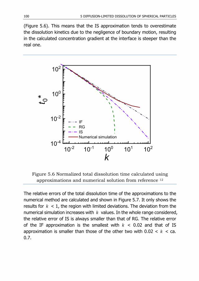
100 5 DIFFUSION-LIMITED DISSOLUTION OF SPHERICAL PARTICLES
(Figure 5.6). This means that the IS approximation tends to overestimate the dissolution kinetics due to the negligence of boundary motion, resulting in the calculated concentration gradient at the interface is steeper than the real one.
Figure 5.6 Normalized total dissolution time calculated using approximations and numerical solution from reference 12
The relative errors of the total dissolution time of the approximations to the numerical method are calculated and shown in Figure 5.7. It only shows the results for k < 1, the region with limited deviations. The deviation from the numerical simulation increases with k values. In the whole range considered, the relative error of IS is always smaller than that of RG. The relative error of the IF approximation is the smallest with k < 0.02 and that of IS approximation is smaller than those of the other two with 0.02 < k < ca. 0.7.
10-2 10-1 100 101 10210-4
10-2
100
102
t 0*
k
IF RG IS Numerical simulation

5.4 APPROXIMATE SOLUTIONS FOR DISSOLUTION OF A SINGLE PARTICLE 101
Figure 5.7 Relative errors of total dissolution time of approximated methods to numerical results
Figure 5.7 can serve as a guideline for the applicable range of the approximations with respect to the total dissolution time. For instance, to control the error below 10 %, IF is appropriate for k < 0.03, RG for k < 0.06, and IS for k < 0.15. All three methods yield reasonable results only for a limited range of k values. In fact, this is the intrinsic limitation of the approximate solutions due to the assumptions made to solve the problem. The IF and IS approximations assume that the interface between the particle and the medium is fixed and the influence of interface motion on the diffusion field is ignored, which means d
d0r
t≈ (5.23)
This will only be approached with reasonable accuracy when
10-2 10-1 1000
10
20
30R
elat
ive
erro
r (%
)
k
IF RG IS

102 5 DIFFUSION-LIMITED DISSOLUTION OF SPHERICAL PARTICLES
( ) ( )P M I MC C C C− − (5.24) which means 0I M
AP M
C CCC C
−= →
− (5.25)
where AC is a supersaturation parameter. The relation between k and AC shows that in this case also k approaches zero. Thus, ( )2 2 01I M A
P I A
C C CkC C C
−≡ = →
− − (5.26)
In addition, the IF approximation treats the dissolution as a quasi-equilibrium process. This assumption is only true when k is extremely small. That is why both the IF and IS approximations are only suitable for conditions with small k and the application range (range of k values) for IF is even smaller than for IS. RG treats dissolution as essentially the reverse of growth. The solution comes from the exact solution for the growth of spherical precipitates and replaces the growth time gt with ( )RG tτ − . For growth, the concentration profile fulfils
2 2 2g
C C CDx x tx
∂ ∂ ∂+ = ∂ ∂∂ (5.27)
and ( )RGddg
tC C Ct t t t
τ −∂ ∂ ∂= = −∂ ∂ ∂
(5.28) Thus, for dissolution, 2 2 2C C CD
x x tx ∂ ∂ ∂+ = − ∂ ∂∂
(5.29) which suggests that the solution does not follow Fick’s second law (Equation (5.1)) and deviates from the exact dissolution kinetics. Only when k is small

5.4 APPROXIMATE SOLUTIONS FOR DISSOLUTION OF A SINGLE PARTICLE 103
and dissolution is slow, the change of concentration profile is accordingly slow 0C
t∂ ≈∂
(5.30) The deviation can be small, and the solution has reasonable accuracy. Another main source of these deviations should be ignoring the convection induced by density differences. Cable et al. (1967) 8 investigated the influence of convection due to the density difference between the two phases, i.e., the solute will not occupy the same volume in the solution as it does in the pure solute. The numerical simulation results8 showed that the influence is less than 10 % up to k = 1.0, while the influence increases progressively with increasing k . Diffusion coefficient is a crucial parameter in a kinetics study. It can be calculated via total dissolution time τ , 0t ′ , or 0t∗ using Equation (5.10), (5.15), or (5.21). The data needed are the total dissolution time τ , initial radius 0r , and k . The first two can be obtained directly from experimental results and k from a simple calculation. The approximate method that estimates the dimensionless total dissolution time 0t∗ best should also be the best option for the estimation of diffusion coefficient. It can be selected using Figure 5.7 with k values for given error levels. Figure 5.5 and Figure 5.7 can be used as references when selecting an appropriate approximation, taking into account experimental uncertainty and desired accuracy. Generally speaking, the IS approximation can be considered to be the best estimation method for two reasons. Firstly, the dissolution curves it produces (Figure 5.4) can reflect the influence of k and are in good agreement with the numerical simulation results. The deviation is less than 8 % for k up to 38 (Figure 5.5). Compared to the other two approximations, the IS approximation reaches the best estimate of the total dissolution time and the diffusion coefficient for 0.02 < k < 0.7 and the relative error is less than 6 % for k < 0.02. On the other hand, the IF approximation needs the least calculation. It can be a good choice when k is extremely small and the error can be controlled well under the desired

104 5 DIFFUSION-LIMITED DISSOLUTION OF SPHERICAL PARTICLES
level. However, the application range of the approximations is limited and none of the approximations gives satisfactory results for large k values.
5.4.2 Applications on Kinetics Studies
5.4.2.1 Dissolution of Alumina Particles in a CaO-Al2O3-SiO2 Melt
o test the validity of the approximations, experimental data from our previous research 15 are employed. The authors observed the dissolution
behavior of spherical alumina particles in a CaO-Al2O3-SiO2 melt using CSLM 15. The experimental setup was similar to that of this work. Another reason to choose the results of reference 15 is that the diffusion coefficients at different temperatures were obtained by combining the experimental observations and lattice Boltzmann model simulations. These data can serve as a good reference for the evaluation of the approximations. Figure 5.8 shows the dissolution curves of Al2O3 particles in a CaO-Al2O3-SiO2 melt at different temperatures. The curves exhibit an “S” shape, indicating a faster dissolution rate at the beginning and at the end than in the middle of the dissolution process. The parameters used to calculate the theoretical dissolution curves and diffusion coefficients are listed in Table 5.1. Since the differences among k values are relatively small, the dissolution curves calculated by the IS approximation are, just like the experimental points, close to each other for different temperatures. Therefore, only three representative experimental results are selected and shown in Figure 5.8. With the values of k around 0.3 to 0.5, the IS approximation can represent the dissolution processes best among the three approximations (as shown in Figure 5.5, the error is smaller than 8 %). The IF and RG approximations deviate considerably from the experimental results (error ca. 20 %). The good agreement between the IS approximation and experimental data indicates that the dissolution of alumina particles in CaO-Al2O3-SiO2 is diffusion controlled. If the experimental results are only compared with the theoretical line of IF or RG, it may exclude diffusion as the rate controlling step.
T

5.4 APPROXIMATE SOLUTIONS FOR DISSOLUTION OF A SINGLE PARTICLE 105
Figure 5.8 Experimental dissolution curves of Al2O3 particles in CaO-Al2O3-SiO2 melt at different temperatures compared with
different approximations
The particle radius and total dissolution time of each experiment are listed in Table 5.2. The diffusion coefficients, as well as the activation energy estimated with these approximations, can also be found in Table 5.2. The physicochemical parameters used in the calculations are listed in Table 5.1. Rather significant variations can be noticed among different approximations for both the diffusion coefficients and activation energies. As shown in Figure 5.7, the deviation can be as high as 30 % for k = 0.6. The relative errors of the diffusion coefficients obtained via the three approximations to the numerical results (given in Table 5.2) are shown in Figure 5.9. Even though the values estimated with the IS approximation are those closest to the simulation results, some of the relative errors are still larger than 10 % (Figure 5.9).
0.0 0.2 0.4 0.6 0.8 1.00.0
0.2
0.4
0.6
0.8
1.0
IF/ RG IS (k = 0.33, 0.36, 0.47) 1743 K 1773 K 1823 K
r / r 0
t / τ

106 5 DIFFUSION-LIMITED DISSOLUTION OF SPHERICAL PARTICLES
Table 5.1 Parameters used for calculating theoretical dissolution curves and diffusion coefficients
System Temperature (K) IC (mol/L) MC (mol/L) PC (mol/L) k p Rλ
Al2O3
1743 9.6 # 5.6 34 * 0.33 0.16 0.40
1773 9.9 # 5.6 34 * 0.36 0.17 0.42
1823 11 # 5.6 34 * 0.47 0.19 0.51
1873 12 # 5.6 34 * 0.59 0.22 0.62
1903 13 # 5.6 34 * 0.66 0.23 0.68
Nd2O3
1141 7.6×10⁻² ## 0 20 ** 7.5×10⁻³ 2.5×10⁻² 4.5×10⁻²
1191 7.5×10⁻² ## 0 20 ** 7.5×10⁻³ 2.4×10⁻² 4.5×10⁻²
1241 7.4×10⁻² ## 0 20 ** 7.4×10⁻³ 2.4×10⁻² 4.5×10⁻²
1291 7.3×10⁻² ## 0 20 ** 7.3×10⁻³ 2.4×10⁻² 4.4×10⁻²
# The saturation concentration was obtained from Ref.3,15, and the density of the melt was calculated according to the data from Ref.22. ## The solubility was obtained from Ref.23, and the density of the melt was calculated according to the data from Ref.24. * The porosity of the particles is assumed to be the same as the Nd2O3 particles made for this study, which is 11%. ** The apparent density was measured by the Archimedes' method.

5.4 RESULTS AND DISCUSSION 107
Table 5.2 Diffusion coefficients obtained via different approximations
System Temperature (K) 0r (μm) τ (s) D (10-10 m2/s) E (102 kJ/mol)
IF IS RG Simulation IF IS RG
Al2O3
1743 250 4450 0.43 0.27 0.22 0.24 $
2.8 2.4 3.2
1743 250 4200 0.45 0.28 0.24 0.25 $
1773 250 3800 0.46 0.29 0.24 0.26 $
1773 250 3580 0.49 0.30 0.25 0.28 $
1823 250 2160 0.62 0.36 0.28 0.33 $
1823 250 1950 0.69 0.40 0.31 0.34 $
1823 250 1825 0.74 0.43 0.33 0.38 $
1873 250 1280 0.83 0.45 0.32 0.42 $
1873 250 1200 0.88 0.48 0.34 0.48 $
1873 250 1340 0.79 0.43 0.31 0.41 $
1903 250 550 1.7 0.92 0.61 0.84 $
1903 250 470 2.0 1.1 0.72 0.97 $
1903 250 720 1.3 0.70 0.47 0.69 $
1903 250 740 1.3 0.68 0.46 0.66 $

108 5 DIFFUSION-LIMITED DISSOLUTION OF SPHERICAL PARTICLES
System Temperature (K) 0r (μm) τ (s) D (10-10 m2/s) E (102 kJ/mol)
IF IS RG Simulation IF IS RG
Nd2O3
1141 292 7371 15 14 14 -
1.2 1.2 1.2 1191 297 5550 21 20 20 -
1241 169 810 48 44 44 -
1291 323 2263 63 59 58 - $ Data are taken from reference 15.
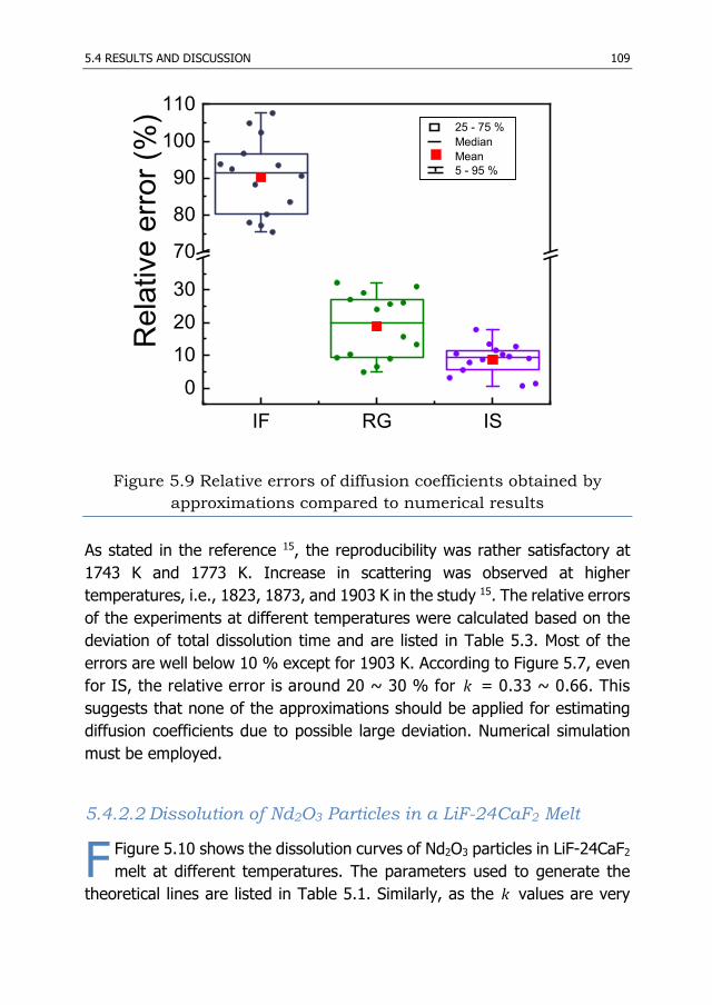
5.4 RESULTS AND DISCUSSION 109
Figure 5.9 Relative errors of diffusion coefficients obtained by approximations compared to numerical results
As stated in the reference 15, the reproducibility was rather satisfactory at 1743 K and 1773 K. Increase in scattering was observed at higher temperatures, i.e., 1823, 1873, and 1903 K in the study 15. The relative errors of the experiments at different temperatures were calculated based on the deviation of total dissolution time and are listed in Table 5.3. Most of the errors are well below 10 % except for 1903 K. According to Figure 5.7, even for IS, the relative error is around 20 ~ 30 % for k = 0.33 ~ 0.66. This suggests that none of the approximations should be applied for estimating diffusion coefficients due to possible large deviation. Numerical simulation must be employed.
5.4.2.2 Dissolution of Nd2O3 Particles in a LiF-24CaF2 Melt
Figure 5.10 shows the dissolution curves of Nd2O3 particles in LiF-24CaF2 melt at different temperatures. The parameters used to generate the
theoretical lines are listed in Table 5.1. Similarly, as the k values are very
IF RG IS0
102030
70
80
90
100
110
Rel
ativ
e er
ror (
%) 25 - 75 %
MeanMedian
5 - 95 %
F

110 5 DIFFUSION-LIMITED DISSOLUTION OF SPHERICAL PARTICLES
Table 5.3 Relative error of the experiments at different temperatures
Temperature (K) 1743 1773 1823 1873 1903
Relative error (%) * 4 4 9 6 21
* Based on the total dissolution time of the experiments conducted at each temperature
Figure 5.10 Dissolution curves of Nd2O3 particles in molten LiF-CaF2 at different temperatures compared with different models
close to each other, the theoretical lines calculated via the IS approximation are hard to be distinguished. The differences among IF, RG and IS are also small. Figure 5.5 suggests that the deviation of the dissolution curves of IF, RG and IS from the numerical simulation is well below 10 % for k = ca. 0.007. Any of the three approximations is capable of representing the step controlling the kinetics. The IF and RG approximations (Equation (5.9) and (5.14)) have a simpler form, and therefore it is easier to generate the
0.0 0.2 0.4 0.6 0.8 1.00.0
0.2
0.4
0.6
0.8
1.0
IF/RG IS (k = 0.0075, 0.0074, 0.0073) Nd2O3 in LiF-CaF2 at 1191 K Nd2O3 in LiF-CaF2 at 1241 K Nd2O3 in LiF-CaF2 at 1291 K
r / r 0
t / τ

5.5 CONCLUSIONS 111
theoretical curve than for the IS approximation. The experimental data at these temperatures are also shown in Figure 5.10, which match the theoretical lines quite well. This suggests that the rate controlling step of dissolution is the diffusion of Nd2O3 in LiF-24CaF2 melt. The diffusion coefficients estimated with these models are listed in Table 5.2. As discussed previously in Section ″Evaluation of Approximations″, the variation among different approximations is negligible with respect to the experimental uncertainty, since the k values are small. The variation of the diffusion coefficients estimated by IF, IS and RG is less than 10% as expected (Table 5.2). The activation energy is calculated to be 1.2×10² kJ/mol for all three approximations. This further indicates that any of the three approximations can fulfil the accuracy requirements. The IF approximation would be recommended here as its solution is the simplest and explicit, and there is no need to solve the implicit Equation (5.13) or (5.20).
5.5 Conclusions
his research provides a systematic evaluation and the applications in real practices of three approximations, i.e., IF, RG, and IS approximations,
describing the diffusion-limited dissolution of a spherical particle in an infinite medium. The conclusions can be drawn as follows: 1) Considering both the generated dissolution curves and estimated
diffusion coefficient, the IS approximation can be considered to be the best estimation method among the three for the physicochemical parameter k < 0.7. All the three approximations can only be applied with limited k values to obtain satisfactory results. Figure 5.5 and Figure 5.7 are the guidelines for determining the applicable ranges.
2) The IF and RG approximations have the identical dissolution curves
independent of k and are only realistic for small k , e.g. k < 0.09 with an error less than 10 %, or k < 0.4 with an error less than 20 %. By contrast, the dissolution curves produced by the IS approximation can reflect the influence of k and agrees well with the numerical simulation results. The deviation is less than 8 % for k up to 38.
T

112 5 DIFFUSION-LIMITED DISSOLUTION OF SPHERICAL PARTICLES
3) Estimating total dissolution time, the three approximations can only be
adequate for small k values. The IF approximation is the best for k < 0.02 and IS approximation is better than the other two for 0.02 < k < ca. 0.7. For all three approximations, the relative errors are larger than 10 % for k > 0.15.
4) The dissolution of alumina particles in CaO-Al2O3-SiO2 is diffusion
controlled. The IS approximation can represent the dissolution processes well. With k = 0.33 ~ 0.66, the deviation of estimated diffusion coefficients by the approximations may be as high as 30 %. None of the approximations is appropriate for this purpose.
5) The rate controlling step of the dissolution of Nd2O3 in LiF-24CaF2 is also
the diffusion of solute in the melt. The differences among the three approximations can be neglected, since k = 0.0073 ~ 0.0075. Any of them can reproduce the experimental data with satisfactory agreement. The errors of the diffusion coefficients obtained should be well below 10 %.

REFERENCES 113
References
1. Ågren J. Kinetics of Carbide Dissolution. Scand. J. Metall. 1990; 19(1): 2-8.
2. Costa P, Manuel J, Lobo S. Modeling and Comparison of Dissolution Profiles. Eur. J. Pharm. Sci. 2001; 13(2): 123-133.
3. Guo X, Sun Z, Van Dyck J, Guo M, Blanpain B. In-Situ Observation on Lime Dissolution in Molten Metallurgical Slags-Kinetic Aspects. Ind. Eng. Chem. Res. 2014; 53(15): 6325-6333.
4. Levenspiel O. Chemical Reaction Engineering. (3rd edition). New York: John Wiley & Sons, 1999.
5. Aaron H, Kotler G. Second Phase Dissolution. Metallurgical Transactions. 1971; 2(2): 393-408.
6. Aaron HB, Fainstei.D, Kotler GR. Diffusion-Limited Phase Transformations - a Comparison and Critical Evaluation of Mathematical Approximations. J. Appl. Phys. 1970; 41(11): 4404-&.
7. Readey DW, Copper AR. Molecular Diffusion with a Moving Boundary and Spherical Symmetry. Chem. Eng. Sci. 1966; 21(10): 917-922.
8. Cable M, Evans DJ. Spherically Symmetrical Diffusion-Controlled Growth or Dissolution of a Sphere. J. Appl. Phys. 1967; 38(7): 2899-&.
9. Tundal UH, Ryum N. Dissolution of Particles in Binary-Alloys .1. Computer-Simulations. Metall. Mater. Trans. A. 1992; 23(2): 433-444.
10. Nojiri N, Enomoto M. Diffusion-Controlled Dissolution of a Spherical Precipitate in an Infinite Binary Alloy. Scr. Metall. Materialia. 1995; 32(5): 787-791.
11. Verhaeghe F, Arnout S, Blanpain B, Wollants P. Lattice-Boltzmann Modeling of Dissolution Phenomena. Phys. Rev. E. 2006; 73(3): 10.
12. Brown LC. Diffusion-Controlled Dissolution of Planar, Cylindrical, and Spherical Precipitates. J. Appl. Phys. 1976; 47(2): 449-458.
13. Sridhar S, Cramb AW. Kinetics of Al2O3 Dissolution in CaO-Mgo-SiO2-Al2O3 Slags: In Situ Observations and Analysis. Metall. Mater. Trans. B. 2000; 31(2): 406-410.
14. Liu J, Guo M, Jones PT, Verhaeghe F, Blanpain B, Wollants P. In Situ Observation of the Direct and Indirect Dissolution of Mgo Particles in

114 5 DIFFUSION-LIMITED DISSOLUTION OF SPHERICAL PARTICLES
CaO-Al2O3-SiO2-Based Slags. J. Eur. Ceram. Soc. 2007; 27(4): 1961-1972.
15. Liu J, Verhaeghe F, Guo M, Blanpain B, Wollants P. In Situ Observation of the Dissolution of Spherical Alumina Particles in CaO-Al2O3-SiO2 Melts. J. Am. Ceram. Soc. 2007; 90(12): 3818-3824.
16. Sun ZHI, Guo X, Van Dyck J, Guo M, Blanpain B. Phase Evolution and Nature of Oxide Dissolution in Metallurgical Slags. AlChE J. 2013; 59(8): 2907-2916.
17. Whelan MJ. On the Kinetics of Precipitate Dissolution. Metal Science. 1969; 3(1): 95-97.
18. Perry DL. Handbook of Inorganic Compounds. (Second edition). Boca Raton, FL: CRC Press, Taylor & Francis Group, 2011.
19. Hideaki I. Semi-Empirical Estimation of Thermal Expansion Coefficients of Oxides. Japanese Journal of Applied Physics. 1996; 35(9R): 4730.
20. Hu X. Study on Ionic Structure and Its Application of NdF3-LiF-Nd2O3 System Melts [Ph.D. Dissertation]. Shenyang, Northeastern University; 2008.
21. Brown LC. Shape Changes During Dissolution of Theta-Cual2. Metall. Mater. Trans. A. 1984; 15(3): 449-458.
22. Bottinga Y, Weill DF. Densities of Liquid Silicate Systems Calculated from Partial Molar Volumes of Oxide Components. Am. J. Sci. 1970; 269(2): 169-&.
23. Guo X, Sun Z, Sietsma J, Yang Y. Semiempirical Model for the Solubility of Rare Earth Oxides in Molten Fluorides. Ind. Eng. Chem. Res. 2016; 55(16): 4773-4781.
24. Porter B, Meaker RE. Density and Molar Volumes of Binary Fluoride Mixtures. Washington: Department of the Interior, Bureau of Mines, 1966.

6
Quantitative Study on Dissolution
Behavior of Nd2O3 in Fluoride
Melts§
Abstract
he dissolution of rare earth oxides in molten fluorides is a critical step in the preparation of the corresponding rare earth metals by oxide-fluoride
electrolysis. However, quantitatively understanding the nature of dissolution, especially in the case of molten salts, is usually difficult to be achieved by post-mortem characterization. In this chapter, the dissolution behavior of Nd2O3 particles in molten fluorides was studied via in-situ observation with a confocal scanning laser microscopy. Combining direct observation with thermodynamic analyses on the oxide dissolution, the rate-limiting step(s), and the effects of conditions like temperature, salt type, and composition on the dissolution rate are identified. This study provides a methodology to estimate the dissolution kinetics of rare earth oxides in molten fluorides during their primary and secondary processing.
§ This Chapter is based on the paper - Guo X, Sun Z, Sietsma J, Blanpain B, Guo M, Yang Y. Quantitative Study on Dissolution Behavior of Nd2O3 in Fluoride Melts. Ind. Eng. Chem. Res. 2018; 57(5): 1380-1388.
T

116 6 QUANTITATIVE STUDY ON DISSOLUTION BEHAVIOR OF ND2O3 IN FLUORIDE MELTS
6.1 Introduction
s its principal application, over 75 % of neodymium is used in the magnet industry1. Since their discovery in 1984, NdFeB magnets have
been outranking all other materials with respect to magnetic flux density2. They have been applied to many advanced technologies, such as miniature high-capacity hard disk drives, compact industrial motors, electric vehicles, and wind turbines2. In 2015, the total amount of rare earth metals (REMs) used in NdFeB magnets was around 25 to 30 kt3. This accounts for 20 % of the total rare earth metals consumption (calculated based on rare earth oxide (REOs)4,5. It is estimated that the global demand for rare earth metals in permanent magnets will increase to 40 kt in 2020, which means that annual growth of 7 % is foreseen3. However, the supply of neodymium is politically sensitive, since practically all rare earth metals are produced in China. Therefore, neodymium is categorized in the most critical raw materials, having the highest supply risk in the commission communication on the 2017 List of Critical Raw Materials for the European Union6. Nowadays, oxide-fluoride electrolysis is the dominant technique for the commercial production of neodymium and its alloys from neodymium oxide in both primary and secondary (recycling) production7. In the process, neodymium oxide is reduced to metal at the cathode. A mixture of fluorides, mostly containing rare earth fluoride (REF), alkali metal fluoride (AF), and possibly small amounts of alkali earth metal fluorides (AEF), serves as both the solvent for neodymium oxide and the electrolyte for the electrolysis8. The electrolysis conditions were found to have significant effects on the process and the current efficiency. One of the critical factors is the feeding rate of neodymium oxide, which needs to be well controlled to ensure smooth production. On the one hand, deficiency of oxide can lead to the generation of fluorocarbon, covering the graphite anode and inhibiting the electrolysis process. On the other hand, overfeeding can cause a sludge of excess oxide at the bottom of the cell, which is detrimental to the quality of the final products. A systematic study on the dissolution behavior of Nd2O3 in molten fluorides can lead to an improved understanding of its dissolution mechanisms and a quantitative description of the dissolution rate, which would provide crucial
A

6.2 EXPERIMENTAL PROCEDURE 117
theoretical support for feeding control in the industrial production. However, research on the interaction between REOs and molten salts is very limited. Stefanidaki et al. (2002) 9 and Hu (2008) 10 studied the products of the interaction between Nd2O3 and fluoride melt with Raman spectroscopy and found the formation of M-O-F (M = metal) complex anions during Nd2O3 dissolution. A previous study11 investigated the interactions of Nd2O3 with molten CaCl2 and CaF2-LiF. It is found that Nd2O3 reacts vigorously with CaCl2 to form NdOCl, while Nd2O3 gradually dissolves in molten CaF2-LiF 11. However, a quantitative discussion of the dissolution process is missing. In the present study, the dissolution of Nd2O3 particles in molten fluorides is investigated with confocal scanning laser microscopy (CSLM), which provides in-situ observation of the dissolution process. This research focuses on understanding the dissolution mechanisms, examining both qualitatively and quantitatively the influencing factors, i.e., temperature, salt type, and composition, and providing a method for predicting the dissolution rate of Nd2O3 in LiF-NdF3.
6.2 Experimental Procedure
6.2.1 Materials
he chemicals used in the CSLM experiments are produced by Alfa Aesar with a purity of 99.95 wt. %. The compositions of the binary salts based
on LiF, NdF3, NaF, and KF are listed in Table 6.1. Prior to the CSLM experiments, the salts were prepared in a horizontal tube furnace. The chemicals were mixed manually and placed in graphite crucibles before being
Table 6.1 Composition of the salts used in this study (mol. %)
Number LiF NdF3 NaF KF
1 77 23
2 90 10
3 95 5
4 23 77
5 23 77
T
118 6 QUANTITATIVE STUDY ON DISSOLUTION BEHAVIOR OF ND2O3 IN FLUORIDE MELTS
loaded into the horizontal furnace. The mixtures were heated up to 50 K above their melting temperatures and held for at least 3 hours before being quenched with liquid nitrogen. These master salts were crushed into small pieces and kept in a glove box before the CSLM tests. The Nd2O3 particles were prepared with the same material and by the same method as described in Chapter 6; the technical details will be omitted here to avoid repetition.
6.2.2 Experimental Apparatus and Procedures
he dissolution of Nd2O3 particles was observed with a CSLM IIF microscope (Lasertec, 1LM21M-SVF17SP), of which the description is
given in Chapter 5 as well. The experiments were conducted in the same manner as described in chapter 6, where the details of the experimental procedure can be found. Figure 6.1 shows a series of CSLM images taken from the experiments, showing the dissolution of a Nd2O3 particle in KF-23NdF3 at 1141 K. The dashed lines indicate the border of the particle. The shrinkage of the particle can be clearly seen in the images. The equivalent radius of the particle can be determined according to the area enclosed by the lines. The upper-left corner of the CSLM images shows the time from the start of the experiment (in seconds) and the measured temperature (in °C). The starting of the dissolution process is at the moment at which the set temperature is reached. The particle size changing with time can be extracted from 50 to 100 CSLM images with specific time intervals. This relationship will be analyzed to reveal the dissolution mechanisms and related kinetic parameters.
6.3 Results and discussion
6.3.1 CSLM in-situ observations
he dissolution of Nd2O3 in all melts studied in this chapter was very similar to that shown in Figure 6.1. The dissolution was gradual, and no
severe reaction was observed. No solid product was formed outside the
T
T

6.3 RESULTS AND DISCUSSION 119
Figure 6.1 CSLM images of the dissolution of Nd2O3 in KF-23NdF3 at 1141 K
particle during dissolution. In some cases, a change of particle shape was noticed, possibly due to differences in dissolution rate at spots with different curvature12. Qualitatively, it is evident that the dissolution from convex areas is more faster than from concave areas, resulting in the spheroidization of particles12. Simulation on the shape change of a four-fold symmetrical precipitate during dissolution confirmed the occurrence of the spheroidization12. With the experimental results published in the same paper,
124.8 um
124.8 um 124.8 um
124.8 um
124.8 um 124.8 um

120 6 QUANTITATIVE STUDY ON DISSOLUTION BEHAVIOR OF ND2O3 IN FLUORIDE MELTS
the author also demonstrated that the theory could be extrapolated to three dimensions and irregular shapes12. The total dissolution time of a four-fold symmetrical precipitate is the same as that of a circular one with the same amount of solute12. Therefore, the equivalent radius is calculated and applied to determine the dissolution mechanisms and related parameters. During the dissolution, the generation of bubbles was observed, as indicated in Figure 6.2 for an experiment at 950°C. The bubbles most likely result from the release of trapped air in the particle. This sometimes triggered the rotation of the particle during the dissolution. To make sure that the experimental conditions are fulfilled within the requirements of the physical model for kinetic study, the experiments were selected excluding those, in which the movement triggered by the release of bubbles was visually significant.
Figure 6.2 Release of bubbles during the dissolution of Nd2O3 particles
124.8 um
Bubble
Bubble

6.3 RESULTS AND DISCUSSION 121
6.3.2 Dissolution Mechanisms
n literature, the fluid is usually assumed to be stagnant when convection is significantly depressed13. In this research, stagnant fluid is assumed
because of the following reasons: 1) the particle movement is observed to be minor; 2) the sample size is relatively small to ensure insignificant temperature gradient in the fluid; 3) the heating source with a high power and a low sample amount enables high heating and cooling rates with almost negligible temperature turbulence once a set temperature is reached. Therefore, it is appropriate to assume that the fluid is stagnant as shown in related references for this type of research14-16. For the dissolution without solid products in a stagnant fluid, the process involves (i) the chemical reaction that transfers atoms or molecules across the phase interface and (ii) the diffusion of solute in the melt17. These two steps determine the dissolution rate. In two limiting cases, the process can be reaction controlled or diffusion controlled. Under the assumption of the chemical reaction controlling the dissolution rate, the relationship between the radius and dissolution time is obtained as18 0 1r t
r τ= − (6.1)
where r and 0r are the actual and original particle radius in m, respectively, t and τ are the actual time and total dissolution time in s, respectively. The
rate of dissolution ( d dr t ) is constant in this case and equal to 0rτ
− .
For diffusion-controlled dissolution that follows Fick’s second law, an exact analytical solution for spheres is not available19. Approximate solutions are alternatives for solving related problems. To select an appropriate approximation20, the supersaturation index k is a crucial physicochemical parameter, expressing the supersaturation ratio, as defined in Equation (5.6).
I

122 6 QUANTITATIVE STUDY ON DISSOLUTION BEHAVIOR OF ND2O3 IN FLUORIDE MELTS
In this study, MC represents the original composition of the melt. As the melt did not contain any Nd2O3 at the beginning, MC is zero under the experimental conditions.
pC represents the density of the solute in the particle, which is taken as a
constant. If the particle contains the solute purely, pC can be calculated directly from the particle density, which is 6.8 g/cm3 in this study, according to
2 3
3 3 3 3
PNd O
g/cm cm /L g/cm cm /L mol/L g/mol
6.8 1000 6.8 1000 20336.5CM
× ×= = = (6.2) For Nd2O3-fluoride systems, the equilibrium concentration can be calculated by 2 3Nd O
Im
sC
V= (6.3)
where 2 3Nd Os is the solubility of Nd2O3 in the melt in mol %, and mV is the
molar volume of the specific mixture in L/mol. The Nd2O3 solubility in molten fluorides is low (see Table 6.2) 21, which means that I PC C (6.4) The value of k can be approximated by
P
I2CkC
≈ (6.5)
Table 6.2 Nd2O3 solubility in LiF-23NdF3
Temperature (K) 868 918 968 1018
Solubility (mol %) 0.24 0.28 0.33 0.38
6.3 RESULTS AND DISCUSSION 123
The values of k for the systems studied in this chapter are listed in Table 6.3. Due to the lack of solubility data for other binary systems, only the k values for LiF-23NdF3 are available. It can be seen that the k values in the systems are always small, and the dissolution in such systems is governed by the concentration profile in a steady state, which is constant with time and is determined by IC , MC , and pC 20. This also suggests that the influence
of the transition period before steady state is negligible. When a small disturbance occurs, the influence of the interruption before the establishment of a new stable concentration field is considered to be insignificant. Excluding the experiments with obvious movement, it is acceptable to hypothesize that the dissolution takes place in a stagnant fluid and the particle position is fixed. The k values are in the range of 0.018 – 0.022, in which the IF approximation is a good choice considering its accuracy to describe a diffusion-controlled process20. In the IF approximation, the relationship between particle radius and time is described by19
1/20 1r tr τ
= −
(6.6) The theoretical dissolution curves of interface reaction (IR) control (Equation (6.1)) and of diffusion control (Equation (6.6)) are shown in Figure 6.3. Comparing the experimental data with theoretical curves reveal the rate-limiting step(s) of the dissolution. The data from the CSLM experiments with LiF-23NdF3 melt at different temperatures are shown in Figure 6.3. It shows that the dissolution of the Nd2O3 particle follows the trend of the diffusion-controlled process. This indicates that the dissolution of a Nd2O3 particle in molten fluorides is diffusion controlled and the IF approximation can be employed to describe the dissolution kinetics.
6.3.3 Diffusion coefficient of Nd2O3 in LiF-NdF3
he total dissolution time in the case of diffusion control can be calculated by19 20r
kDτ = (6.7) T

124 6 QUANTITATIVE STUDY ON DISSOLUTION BEHAVIOR OF ND2O3 IN FLUORIDE MELTS
Table 6.3 Summary of experimental conditions and related parameters
Melt T (K) IC (mol/L) MC (mol/L) pC (mol/L) k 0r (μm) τ (s) kD (10-10m2/s) D (10-10m2/s)
LiF-23NdF3 1141 0.18$ 0 20 0.017 233 1210 0.45 26
LiF-23NdF3 1191 0.20$ 0 20 0.019 312 1486 0.65 34
LiF-23NdF3 1241 0.21$ 0 20 0.021 309 902 1.1 49
LiF-23NdF3 1291 0.22$ 0 20 0.023 338 851 1.3 59
LiF-20NdF3 1241 0.20* 0 20 0.021* 279 772 1.01 49#
LiF-15NdF3 1241 0.15* 0 20 0.015* 258 900 0.74 49#
LiF-10NdF3 1241 0.14* 0 20 0.014* 265 1026 0.68 49#
LiF-5NdF3 1241 0.03* 0 20 0.003* 235 3439 0.16 49#
NaF-23NdF3 1141 - 0 20 - 240 1827 0.32 -
KF-23NdF3 1141 - 0 20 - 243 5338 0.11 - $ The solubility was obtained from reference22 and the density of the melt was calculated according to the data from reference10. # Values are taken from that in LiF-23NdF3 at 1241 K. * Values are calculated assuming that the diffusion coefficient is independent of composition and is the same as that in LiF-23NdF3 at 1241 K.

6.3 RESULTS AND DISCUSSION 125
Figure 6.3 Dissolution curves of Nd2O3 particles in fluoride melts
In this chapter, the Nd2O3-fluoride system is treated as a quasi-binary system of a solute (Nd2O3) and a solvent (the binary melt). The diffusion coefficient D represents the effective diffusion of Nd2O3 in the melt. With the experimental data, including the total dissolution time, original particle radius, and k values, it is possible to calculate the diffusion coefficients (see Table 6.3 and Figure 6.4). As expected, the diffusion coefficients increase with temperature, indicating enhanced diffusion at high temperature. The diffusion coefficient correlates with temperature, following the Arrhenius' equation A0 exp ED D
RT = −
(6.8) where 0D is the pre-exponential factor in m2/s, and AE is the activation energy for diffusion in J/mol.
0.0 0.2 0.4 0.6 0.8 1.00.0
0.2
0.4
0.6
0.8
1.0
IF IR Nd2O3 in LiF-23NdF3 at 1241 K Nd2O3 in LiF-23NdF3 at 1291 K Nd2O3 in LiF-23NdF3 at 1141 K Nd2O3 in KF-23NdF3 at 1141 K
r / r 0
t / τ

126 6 QUANTITATIVE STUDY ON DISSOLUTION BEHAVIOR OF ND2O3 IN FLUORIDE MELTS
Figure 6.4 Experimental values (symbols) for the diffusion coefficient of Nd2O3 in molten LiF-23NdF3, fitted with Equation (6.9)
(solid line)
The fit of Equation (6.8) to the experimental data in Figure 6.4 yields an activation energy of 68 kJ/mol for diffusion and a pre-exponential factor 0D = 3.2×10⁻⁶ m2/s. Thus, in LiF-23NdF3, the diffusion coefficient of Nd2O3 can be calculated by
2 3Nd O
Jm mols426 6.8 103.2 10 expD
RT− ×= × × −
(6.9)
With the k values and Equation (6.9), it is possible to estimate the total dissolution time of Nd2O3 particles in LiF-23NdF3 in the temperature range of 1141 – 1291 K. These parameters are also essential for the numerical simulations of more complex processes, for instance, the dissolution of feed materials in an industrial electrolytic cell with forced mixing effects introduced by generated CO and CO2 bubbles at the anodes during electrolysis.
0.75 0.80 0.85 0.9020
55
Experimental data Fitted Curve
Diff
usio
n C
oeffi
cien
t (10
-10 m
2 /s)
1/T (10-3 K-1)

6.3 RESULTS AND DISCUSSION 127
For dilute solutions, the diffusion coefficient is often viewed as a parameter that is independent of composition. The Nd2O3 solubility in LiF-NdF3 is quite low, and it is, therefore, reasonable to assume that the diffusion coefficient remains unchanged in LiF-NdF3 melts with different NdF3 concentrations. To validate this hypothesis, the Nd2O3 solubility is calculated, assuming that the diffusion coefficient is independent of salt composition. The results are listed in Table 6.3 and shown in Figure 6.5. Assuming a linear relationship of the solubility to NdF3 concentration yields a rather good fit (R2 = 0.97). The gap between the data point for the NdF3 concentration of 10 mol% and the fitted line suggests that this is a bad datum. The linear relationship agrees well with the conclusion from reference21, and confirms that a composition-independent diffusion coefficient is a valid assumption. With this conclusion, it is possible to extend the application of the diffusion coefficient obtained previously. This means that Equation (6.9) can be applied to estimate the diffusion coefficient of Nd2O3 in LiF-NdF3 melts with 5 – 23 mol. % NdF3 at 1141 – 1291 K.
Figure 6.5 Solubility of Nd2O3 in LiF-NdF3 at 1241 K
0 5 10 15 20 250.0
0.1
0.2
0.3
0.4
Nd 2O
3 Sol
ubilit
y (m
ol.%
)
NdF3 Concentration (mol.%)
Nd2O3 Solubility (mol.%) Fitted line

128 6 QUANTITATIVE STUDY ON DISSOLUTION BEHAVIOR OF ND2O3 IN FLUORIDE MELTS
6.3.4 Influencing Factors
6.3.4.1 Temperature
ccording to Equation (6.7), the total dissolution time is inversely proportional to the value of kD , suggesting that Nd2O3 particles dissolve
faster in the melts with higher kD values. The factors that influence the diffusion coefficient D and supersaturation ratio k determine the dissolution rate. In this study, the diffusion coefficient is a function of temperature and is independent of salt composition (Equation (6.9)). According to the definition of k (Equation (6.5)), it is a parameter correlated to the solubility of Nd2O3, molar volume, and composition of the melt. The Nd2O3 solubility and melt density are functions of temperature and salt composition. Thus, the influence of these factors, i.e., temperature and salt composition, will be discussed based on the experimental observations in the following paragraphs. The product of D and k in LiF-23NdF3 at different temperatures have been derived by means of Equation (6.7) from the observed completion time τ in combination with the initial radius 0r . The results are shown in Figure 6.6. The kD values increase with temperature, suggesting that the dissolution rate is enhanced at elevated temperatures. The effects of temperature on the diffusion coefficient are given in Equation (6.9). According to the experimental conditions, Nd2O3 was not present in the original melts, i.e., MC = 0. The influences on the k values merely reflect the variations of the solubility and molar volume among the studied systems. The previous research22 shows that the relationship between solubility and temperature can be expressed as
2 3Nd O exp As XRT
= −
(6.10) where X is a function related to the melt composition, and A is a positive constant in J/mol. For LiF-NdF3 melt22, the Nd2O3 solubility can be calculated by 22
A

6.3 RESULTS AND DISCUSSION 129
Figure 6.6 Product kD , determining Nd2O3 dissolution in LiF-23NdF3, as a function of temperature ( )2 3 3Nd O NdF LiF
kJ/molmol.% 40( ) 1.1 0.12 exps x xRT
= − −
(6.11) where ix is the mole fraction of compound i in the original melt without dissolved Nd2O3. It is readily established that the Nd2O3 solubility in LiF-NdF3 increases with temperature. The melt density has a linear relationship with temperature, expressed as23 a bTρ = − (6.12) where ρ is the melt density in kg/m3 at temperature T , a and b are two positive constants. The relationship shown in Equation (6.12) is valid for both pure compounds and mixtures. The values of a and b depend on melt composition. The molar volume is correlated to the density by
1150 1200 1250 1300
0.4
0.6
0.8
1.0
1.2
1.4
kD (1
0-10 m
2 /s)
Temperature (K)

130 6 QUANTITATIVE STUDY ON DISSOLUTION BEHAVIOR OF ND2O3 IN FLUORIDE MELTS
mMVρ
= (6.13) where M is the molecular mass. According to Equation (6.12) and (6.13), the melt density decreases with temperature, while the molar volume increases with temperature. The solubility of Nd2O3 in fluorides is limited, usually far less than 1 mol. %22. Its influence on the molar volume of the salts can be ignored. In this chapter, the solution with dissolved Nd2O3 will be treated as a quasi-binary salt system for density calculations. Due to the lack of the density data for LiF-NdF3 melts, its molar volume will be calculated from the density of pure LiF and NdF3. The molar volume mV of an ideal binary mixture can be calculated by m m1 m21 2V x V x V= + (6.14) where m1V and m2V are the molar volumes and 1x and 2x the fractions of the respective components. For AF-RF3 binary systems containing LiF, the real values agree quite well with the estimated values from ideal mixtures23. In this chapter, all binary salts will be treated as ideal mixtures when calculating their molar volumes. The values of the parameters in Equation (6.12) are obtained for LiF and NdF3 from reference10, see Table 6.4. These parameters are used for calculating the molar volume of LiF and NdF3 at different temperatures. Combining Equation (6.11) to (6.14) and parameters in Table 6.4, the k values in LiF-NdF3 with different NdF3 concentrations and at different
Table 6.4 Parameters for calculating the density of LiF and NdF3
a# (g/cm3) b# (10-3g/(cm3·K))
LiF 12 7.5
NdF3 9.0 2.9 # Calculated from data in reference 10

6.3 RESULTS AND DISCUSSION 131
temperatures are calculated and shown in Figure 6.7. It is clear that the k values increase with temperature in the considered temperature and composition range. As shown in Figure 6.4 and Figure 6.7, both k and D in LiF-NdF3 melt increase with temperature in the temperature range of this study. Increasing temperature therefore accelerates the dissolution of Nd2O3 in LiF-NdF3 melt. With the increase in NdF3 content, the dependence of k on temperature becomes more significant (Figure 6.7). This influence extends to the dissolution rate, and the temperature has more impacts on the dissolution rate in the melt with higher NdF3 content.
Figure 6.7 Calculated k values in LiF-NdF3 with different NdF3
concentrations and at different temperatures
6.3.4.2 NdF3 Concentration
he dissolution of Nd2O3 in LiF-NdF3 melts with different NdF3 concentrations was observed, and the results show that increasing NdF3
concentration can accelerate the dissolution (see Table 6.3). It is found that
1000 1200 14000.00
0.01
0.02
0.03
0.04
0.05
0.06
k
Temperature (K)
LiF-15NdF3
LiF-23NdF3
LiF-30NdF3
LiF-40NdF3
LiF-50NdF3
T

132 6 QUANTITATIVE STUDY ON DISSOLUTION BEHAVIOR OF ND2O3 IN FLUORIDE MELTS
the kD values increase with increasing NdF3 concentration as shown in Figure 6.8.
Figure 6.8 Experimental values of kD as a function of NdF3 concentration in LiF-NdF3 at 1241 K (the solid line is a guide to the
eye)
As discussed previously, the diffusion coefficient is independent of the salt composition. Therefore, the influence of NdF3 concentration mainly acts on the k values, more precisely, on the Nd2O3 solubility and molar volume of the melt. According to Equation (6.10) and (6.11), the Nd2O3 solubility is proportional to the NdF3 concentration in a LiF-NdF3 melt 21. Although Equation (6.11) is not suitable to estimate the solubility in LiF-NdF3 with a NdF3 concentration lower than 10 mol. %, the proportional relationship between the solubility and NdF3 concentration is retained21. Thus, the solubility can be expressed as
5 10 15 20 250.0
0.2
0.4
0.6
0.8
1.0
1.2kD
(10-1
0 m2 /s
)
NdF3 Concentration (mol. %)
Nd2O3 in LiF-NdF3 at 1241 K Trend line

6.3 RESULTS AND DISCUSSION 133
2 3 3Nd O NdFs m nx= + (6.15)
where m and n are constants. Per Equation (6.14), the molar volume of LiF-NdF3 can be calculated by ( ) ( ) ( ) ( ) ( ) ( )( )3 33 3 3LiF NdF NdFm LiF NdF m LiF m NdF m LiF m NdF m LiFV x V x V V V V x− = + = + − (6.16) where the molar volume of LiF and NdF3, i.e., ( )m LiFV and ( )3m NdFV , can be
obtained based on the data in Table 6.4. Therefore, the composition dependence of k can be expressed as
( ) ( ) ( )( )( ) ( ) ( )( )
3
3 333
m LiF m NdF m LiF
NdF P NdF PNdFm LiF m NdF m LiF
I 22 2 nV m V VCk cx C x C V V V x
− −∂∂ = ⋅ = ⋅ =∂ ∂ + −
(6.17) Thus, ( )
3 3NdF NdF
kD kD cDx x
∂ ∂= =∂ ∂
(6.18) The experimental results (Table 6.3 and Figure 6.8) show that the value of
kD increases with NdF3 concentration, which indicates that 3NdF
kcx∂=
∂ is
positive. In addition, c is a parameter decreasing with increasing NdF3 concentration, indicating that the gradient of the curve of the supersaturation index as a function of the NdF3 fraction decreases with increasing concentration. The shape of the trend line in Figure 6.8 is consistent with this conclusion.
6.3.4.3 Alkali Metal Fluorides
Figure 6.9 shows the influence of the type of AF on Nd2O3 dissolution in AF-23NdF3. The dissolution rate decreases in the order from LiF-23NdF3,
NaF-23NdF3, to KF-23NdF3. This supports the choice of LiF-NdF3 as an electrolyte in commercial production concerning the dissolution rate. The molar volumes of LiF, NaF, and KF at a specific temperature increase in the order of their atom number, i.e., ( ) ( ) ( )m LiF m NaF m KFV V V< < 23. According to
F

134 6 QUANTITATIVE STUDY ON DISSOLUTION BEHAVIOR OF ND2O3 IN FLUORIDE MELTS
Figure 6.9 Influence of type of AF on Nd2O3 dissolution in AF-23NdF3 at 1141 K
Equation (6.14), it can be derived that ( ) ( ) ( )3 33m LiF-23NdF m NaF-23NdF m KF-23NdFV V V< < (6.19) The solubility of REOs is found to be associated with the charge density of the cations in the melt22. With higher charge density, it is more likely to form stable M-O-F (M = metal) complex anions, which are the products of the interaction between Nd2O3 and the fluoride melt22. Higher concentration of M-O-F complex in the Nd2O3-fluoride system means that the melt dissolves more Nd2O3. The concentration of NdF3 is the same in these three melts. As indicated in reference22, the charge density decreases in the order from Li+, Na+, and to K+. Given the same Nd3+ concentration, it can be inferred that the Nd2O3 solubility decreases in the order from LiF-23NdF3, NaF-23NdF3, and to KF-23NdF3, i.e.,
LiF-23NdF 3
NaF-23NdF 3
KF-23NdF 3
0.0
0.1
0.2
0.3
0.4
0.5
kD (1
0-10 m
2 /s)

6.4 CONCLUSIONS 135
3 3 3LiF-23NdF NaF-23NdF KF-23NdFs s s> > (6.20)
According to Equation (6.3), this implies ( ) ( ) ( )3 3I LiF-23NdF I NaF-23NdF I KF-23NdF3C C C> > (6.21) As per its definition (Equation (6.5)), the parameter k of the systems follows the order
3 3 3LiF-23NdF NaF-23NdF KF-23NdFk k k> > (6.22) Since absolute k values are not available, it is not possible to obtain the diffusion coefficient of Nd2O3 in NaF/KF-23NdF3. Nevertheless, the dissolution experiments in this study confirm that LiF-NdF3 is a suitable solvent for Nd2O3 regarding kinetic aspects. Also, the solubility in LiF-NdF3 is higher than that in NaF/KF-23NdF3, which means that the former is a better solvent considering the thermodynamic factor. As an electrolyte, the addition of LiF can improve the electrical conductivity of the melt due to the low resistance of movement and high mobility of Li+ cations10. Considering all these advantages, LiF-NdF3 is justifiably chosen as the primary electrolyte for electrowinning neodymium in industrial production.
6.4 Conclusions
n this research, the dissolution behavior of Nd2O3 particles in molten fluorides salts was investigated via in-situ observation with CSLM,
providing a better understanding of the dissolution mechanisms and its influencing factors, i.e., temperature, salt type, and composition. The outcome of the study offers a convenient method to estimate the dissolution time in LiF-NdF3 melt. The main conclusions can be formulated as follows. 1) The dissolution of Nd2O3 in molten fluoride is a diffusion-controlled
process. The diffusion coefficient increases from 2.6×10⁻⁹ to 5.9×10⁻⁹ m2/s when the temperature rises from 1141 to 1291 K, and the activation energy is determined to be 68 kJ/mol.
2) Increasing temperature and NdF3 concentration in LiF-NdF3 melt can
accelerate the dissolution, while LiF-23NdF3 is shown to be a better
I

136 6 QUANTITATIVE STUDY ON DISSOLUTION BEHAVIOR OF ND2O3 IN FLUORIDE MELTS
solvent for Nd2O3 than NaF-23NdF3 and KF-23NdF3 regarding the dissolution rate.
3) The activation energy for diffusion AE and the pre-exponential factor 0D
obtained are two critical parameters in this kinetic study. Together with solubility and density data, it is possible to estimate the total dissolution time of Nd2O3 in LiF-NdF3 melt with 5 – 23 mol.% NdF3 in the temperature range of 1141 – 1291 K.

REFERENCES 137
References
1. Goonan TG. Rare Earth Elements--End Use and Recyclability. Reston: US Department of the Interior, US Geological Survey, 2011.
2. Tanaka M, Oki T, Koyama K, Narita H, Oishi T. Recycling of Rare Earths from Scrap. In: Jean-Claude GB, Vitalij KP, eds. Handbook on the Physics and Chemistry of Rare Earths. Vol 43. Amsterdam: Elsevier, 2013:159-211.
3. Rollat A, Guyonnet D, Planchon M, Tuduri J. Prospective Analysis of the Flows of Certain Rare Earths in Europe at the 2020 Horizon. Waste Manage. (Oxford). 2016; 49: 427-436.
4. Sun Z, Cao H, Xiao Y, Sietsma J, Jin W, Agterhuis H, Yang Y. Toward Sustainability for Recovery of Critical Metals from Electronic Waste: The Hydrochemistry Processes. ACS Sustain. Chem. Eng. 2017; 5(1): 21-40.
5. Sun Z, Xiao Y, Sietsma J, Agterhuis H, Yang Y. Recycling of Metals from Urban Mines – a Strategic Evaluation. J. Cleaner Prod. 2016; 112: 2977-2987.
6. European Commission. Commission Communication on the 2017 List of Critical Raw Materials for the Eu. Brussels: European Commission; 2017.
7. Krishnamurthy N, Gupta CK. Extractive Metallurgy of Rare Earths: CRC press, 2004.
8. Pang S, Yan S, Li Z, Chen D, Xu L, Zhao B. Development on Molten Salt Electrolytic Methods and Technology for Preparing Rare Earth Metals and Alloys in China. Chin. J. Rare Met. 2011; 35(3): 440-450.
9. Stefanidaki E, Photiadis GM, Kontoyannis CG, Vik AF, Ostvold T. Oxide Solubility and Raman Spectra of NdF3-LiF-KF-MgF2-Nd2O3 Melts. J. Chem. Soc., Dalton Trans. 2002; (11): 2302-2307.
10. Hu X. Study on Ionic Structure and Its Application of NdF3-LiF-Nd2O3 System Melts [Ph.D. Dissertation]. Shenyang, Northeastern University; 2008.
11. Mukherjee A, Dyck J, Blanpain B, Guo M. Cslm Study on the Interaction of Nd2O3 with CaCl2 and CaF2-LiF Molten Melts. J. Mater. Sci. 2017; 52(3): 1717-1726.

138 6 QUANTITATIVE STUDY ON DISSOLUTION BEHAVIOR OF ND2O3 IN FLUORIDE MELTS
12. Brown LC. Shape Changes During Dissolution of Theta-Cual2. Metall. Mater. Trans. A. 1984; 15(3): 449-458.
13. Cooper AR, Kingery WD. Dissolution in Ceramic Systems: I, Molecular Diffusion, Natural Convection, and Forced Convection Studies of Sapphire Dissolution in Calcium Aluminum Silicate. J. Am. Ceram. Soc. 1964; 47(1): 37-43.
14. Liu J, Verhaeghe F, Guo M, Blanpain B, Wollants P. In Situ Observation of the Dissolution of Spherical Alumina Particles in CaO-Al2O3-SiO2 Melts. J. Am. Ceram. Soc. 2007; 90(12): 3818-3824.
15. Verhaeghe F, Liu J, Guo M, Arnout S, Blanpain B, Wollants P. Dissolution and Diffusion Behavior of Al2O3 in a CaO-Al2O3-SiO2 Liquid: An Experimental-Numerical Approach. Appl. Phys. Lett. 2007; 91(12): 124104.
16. Feichtinger S, Michelic SK, Kang YB, Bernhard C. In Situ Observation of the Dissolution of SiO2 Particles in CaO-Al2O3-SiO2 Slags and Mathematical Analysis of Its Dissolution Pattern. J. Am. Ceram. Soc. 2014; 97(1): 316-325.
17. Aaron H, Kotler G. Second Phase Dissolution. Metallurgical Transactions. 1971; 2(2): 393-408.
18. Levenspiel O. Chemical Reaction Engineering. (3rd edition). New York: John Wiley & Sons, 1999.
19. Aaron HB, Fainstei.D, Kotler GR. Diffusion-Limited Phase Transformations - a Comparison and Critical Evaluation of Mathematical Approximations. J. Appl. Phys. 1970; 41(11): 4404-&.
20. Guo X, Sietsma J, Yang Y, Sun Z, Guo M. Diffusion-Limited Dissolution of Spherical Particles: A Critical Evaluation and Applications of Approximate Solutions. AlChE J. 2017; 63(7): 2926-2934.
21. Guo X, Sietsma J, Yang Y. A Critical Evaluation of Solubility of Rare Earth Oxides in Molten Fluorides. In: de Lima IB, Filho WL, eds. Rare Earths Industry. Boston: Elsevier, 2016:223-234.
22. Guo X, Sun Z, Sietsma J, Yang Y. Semiempirical Model for the Solubility of Rare Earth Oxides in Molten Fluorides. Ind. Eng. Chem. Res. 2016; 55(16): 4773-4781.
23. Porter B, Meaker RE. Density and Molar Volumes of Binary Fluoride Mixtures. Washington: Department of the Interior, Bureau of Mines, 1966.

7
Electrochemical Behavior of
Neodymium (III) in Molten
Fluorides
Abstract
he electrochemical behavior of trivalent neodymium (Nd(III)) in molten LiF-CaF2 is studied with cyclic voltammetry, square wave voltammetry,
and chronopotentiometry. Two sorts of neodymium compounds, Nd2O3 and NdF3, are applied as the source of Nd(III) in the fluoride electrolyte. The results show that the cathodic process of Nd(III) reduction is diverse in these two systems. The reduction of Nd2O3 in LiF-CaF2 involves two steps, i.e., Nd(III) e Nd(II)+ → and Nd(II) e Nd(0)2+ → . The first step is a reversible and diffusion-controlled reaction. On the other hand, the electrochemical reduction of Nd(III) in LiF-CaF2-NdF3 is a single reaction with three exchanged electrons. The process is quasi-reversible and diffusion-controlled. The potentiostatic electrolysis demonstrates that the electrowinning of neodymium metal can be achieved in LiF-CaF2-Nd2O3 system. An alloy mainly containing neodymium was obtain by constant potential electrolysis from a rare earth oxide mixture that was concentrated from secondary resources,
T

140 7 ELECTROCHEMICAL BEHAVIOR OF NEODYMIUM (III) IN MOLTEN FLUORIDES
which confirms the feasibility of the recovery of rare earth elements from secondary resources.
7.1 Introduction
ince the 1990s, the demand for neodymium has been substantially boosted by the rapid development of NdFeB magnet industry 1. Due to
its essential role in advanced technologies, neodymium is categorized as one of the most critical raw materials 2-4. Nowadays, neodymium is mainly produced by molten salt electrolysis from two types of systems: NdCl3-KCl and NdF3-LiF-BaF2-Nd2O3 1. The former has been taken over progressively by the latter due to its high energy consumption, low current efficiency, and low yield resulted from the high volatility of chlorides and high solubility of neodymium in the electrolyte 1. It is known that the current efficiency or energy consumption is significantly influenced by current and electricity supply. Understanding the path of electron transfer during rare earth oxides (REOs) electrolysis is critical in order to eliminate side reactions and achieve precise control of the process, which can significantly reduce the energy consumption. Unfortunately, even though the molten salt electrolysis has been adopted for the commercial production of neodymium for several decades since 1961 5, the reduction mechanism of Nd(III) is not fully understood. There have already been a number of efforts carried out in literature aiming to provide clarify the reduction process during electrolysis. The study on the electrochemical behavior of NdCl3 in molten LiCl-KCl found that the reduction of Nd(III)/Nd(0) involved two successive steps, i.e., Nd(III) was converted into soluble Nd(II) and then reduced to metallic Nd(0) 6-9. Lu et al. (1991) 10 considered that in molten KCl-NaCl-NdCl3 with the presence of neodymium metal, the cathodic reaction was Nd(II) e Nd2+ → . Novoselova et al. (2013) 11 had a similar conclusion for the cathodic process of NdCl3 in fused eutectic LiCl-KCl-CsCl and pure CsCl. Yamana et al. (2006) 7 further confirmed the presence of Nd(II) by means of UV-visible absorption spectrophotometry.
S

7.1 INTRODUCTION 141
One exception is the work done by Wu et al. (1994) 12, who proposed a three-electron reaction on a gold working electrode in NdCl3-LiCl-KCl melt. The work on fluoride system shows more discrepancies. For some studies in LiF-CaF2 13,14 and pure LiF 15, a two-step mechanism with Nd(II) as intermediate valence was found. Whereas, the findings from other research showed that the electrochemical reduction of Nd(III) in LiF-KF 16, LiF 17 and LiF-CaF2 18, is a one-step reaction exchanging three electrons (Nd(III) e Nd(0)3+ → ). In the industrial production of neodymium, Nd2O3 is added to a mixture of LiF-NdF3 as raw materials. Stefanidaki et al. (2001) 17 reported that the cathodic process recorded by cyclic voltammetry in LiF-NdF3-Nd2O3 was similar to that in LiF-NdF3 system. According to Lu et al. (1991) 13, the cyclic voltammogram of LiF-CaF2-NdF3 with saturated Nd2O3 was almost identical to that of LiF-CaF2-NdF3 without Nd2O3, with slight differences in the deposition potential of neodymium. These results were considered to arise from the much higher concentration of NdF3 than that of Nd2O3 in the melt with saturated Nd2O3 17. The electrochemical signals of Nd2O3 may have been hidden from that of NdF3. This makes the cyclic voltammograms recorded in these two systems look almost the same, which should be avoided when the reduction of Nd2O3 is the focus. In order to provide an in-depth understanding of Nd(III) reduction in molten fluorides, the present research focuses on the electrochemical behavior of Nd(III) in molten LiF-CaF2. Without NdF3 in the system, LiF-CaF2, as a solvent for Nd2O3, can eliminate the influence of NdF3, which would benefit the observation of Nd(III) reduction. In addition, LiF-CaF2 melt can provide a larger electrochemical window than other fluoride mixtures 18. The results are compared with the electrochemical behavior of NdF3 in LiF-CaF2 to have a full picture of Nd(III) reduction from both oxide and fluoride. In addition, this research is part of an EU project (REEcover). The whole project focuses on developing, demonstrating and assessing the economic viability of the recovery of rare earth elements (REEs), including terbium (Tb), dysprosium (Dy), neodymium (Nd), and yttrium (Y), which are especially critical to the European economy, from two types of industrial wastes, i.e.,

142 7 ELECTROCHEMICAL BEHAVIOR OF NEODYMIUM (III) IN MOLTEN FLUORIDES
tailings from the iron ore industry and magnetic waste material from WEEE recycling industry. These two types of waste are upgraded via physical separation and hydrometallurgical or pyrometallurgical treatment. The upgrading materials are then concentrated via solvent extraction to further remove impurities. The end product is a mixture of REOs with minor impurities, which is the raw materials for electrolysis to extract REEs from their oxide form. In this chapter, the possibility of extracting REEs from the concentrated mixture is demonstrated by electrolysis experiments performed in molten LiF-NdF3 melt.
7.2 Experimental
7.2.1 Electrochemical behavior
7.2.1.1 Materials and electrolytic cell
he eutectic composition of LiF-CaF2 binary system is 76 mol. % LiF and 24 mol. % CaF2. Therefore, a mixture containing 76 mol. % LiF (Alfa
Aesar 99.5 wt. %) and 24 mol. % CaF2 (Sigma-Aldrich 99.0 wt. %) was used as the electrolyte for investigating the reduction behavior of Nd2O3 (Solvay Rhodia 99.5 wt. %) in molten fluorides. The melting temperature of the fluoride mixture is 1023 K 19. The experiments were performed at 1123 ‒ 1273 K to guarantee good fluidity and sufficient concentration of dissolved Nd2O3. The amount of added Nd2O3 in the electrolyte was at least triple its solubility at the temperature, which makes sure the concentration of Nd2O3 was always over-saturated. When the melt was in equilibrium, the concentration of Nd2O3 in LiF-24CaF2 should have been its solubility at that temperature (saturation). For comparison, NdF3 (Alfa Aesar 99.9 wt. %) was used to replace Nd2O3 in some experiments. Before experiments, all the chemicals were dehydrated by heating under an argon atmosphere at 673 K for at least 12 hours. The experimental setup is shown in Figure 7.1. A graphite crucible with an inner diameter of 35 mm containing the mixture of electrolyte and Nd2O3 was placed at the hot zone of a vertical furnace. The electrodes were introduced from the top. The distance between the working electrode and counter
T

7.2 EXPERIMENTAL 143
electrode was fixed to 20 mm to eliminate possible influences of distance on the electrochemical reactions. The experiments were performed under an inert argon atmosphere. The temperature was measured using a K-type thermocouple, which touched the bottom of the graphite crucible from the bottom of the furnace.
Figure 7.1 Schematic illustration of the apparatus for electrochemical experiments (inner diameter of graphite crucible: 35
mm)
Off-gases
Reactor
Electrolyte
Graphite Crucible
Argon Thermocouple
Pt electrodeMo electrode
Graphite electrode
Princeton Parstat

144 7 ELECTROCHEMICAL BEHAVIOR OF NEODYMIUM (III) IN MOLTEN FLUORIDES
The working electrode was a molybdenum wire with a diameter of 2 mm. The reaction surface was determined after each experiment by measuring the depth immersed in the melt. The counter electrode was a graphite rod with a diameter of 5 mm, which was connected a molybdenum wire to be extended outside the reactor. A 1-mm diameter platinum wire acted as a quasi-reference electrode in the experiments 20.
7.2.1.2 Techniques
he electrochemical behavior was studied with cyclic voltammetry, square wave voltammetry, and chronopotentiometry, which were performed
using a Princeton Parstat 4000 controlled by a computer using the software VersaStudio 2.52.3. After constant potential electrolysis, the cathode covered with a thin layer of metal and trapped salts was cut off, and its cross section was examined by a scanning electronic microscope (SEM, JEOL JSM 650F).
7.2.2 Constant potential electrolysis
7.2.2.1 Materials and electrolytic cell
he synthetic feed was used as raw material for constant potential electrolysis. The concentrated material mainly contains REOs (ca. 95
wt.%), including Nd2O3, Pr6O11, Dy2O3 (see Table 7.1). The main impurity is manganese oxide, which comes from the remaining impurity in the waste stream. For simplicity, the mixture is called "REO mixture" hereinafter.
Table 7.1 Composition of synthetic feed
REO Pr6O11 Nd2O3 Dy2O3 Total
Concentration (wt.%)
6.44% 85.20% 2.47% 94.12%
T
T

7.2 EXPERIMENTAL 145
A mixture containing 77 mol. % LiF (Alfa Aesar 99.5 wt. %) and 23 mol. % NdF3 (Sigma-Aldrich 99.0 wt. %) was used as an electrolyte. Its melting temperature is around 1011 K 19. Before being loaded to a graphite crucible, the fluorides were well mixed with the REO mixture. The amount of the REO mixture in the electrolyte is always over-saturated in order to prevent oxide depletion during electrolysis process. The mixture was hold at 673K for overnight before electrolysis in order to remove any possible moisture or adsorptive water. The experiments were conducted in a vertical tube furnace under an inert argon atmosphere. The electrodes were introduced from the top. The temperature was measured using a k-type thermocouple, which contacted the bottom of the graphite crucible from the bottom of the furnace. Two-electrode system was used in the experiments. The experimental setup was similar to that shown inFigure 7.1 except for only two electrodes being used. The working electrode was a 2-mm diameter molybdenum wire. The contact area was determined after each experiment by measuring the immersion depth in the bath. A graphite rod with diameter of 10 mm acted as a quasi-reference electrode and a counter electrode.
7.2.2.2 Techniques
he electrolysis were performed using a Princeton Parstat 4000 controlled by a computer using the software VersaStudio 2.52.3.
After constant potential electrolysis, the cathode was covered with a thin layer of metal and trapped salts. To investigate this metallic layer, the electrodes were cut off, and the cross section was subject to EDS analysis with a scanning electronic microscope (SEM, JEOL JSM 650F).
T

146 7 ELECTROCHEMICAL BEHAVIOR OF NEODYMIUM (III) IN MOLTEN FLUORIDES
7.3 Results and discussion
7.3.1 Electrochemical reduction of Nd(III) in molten fluorides
7.3.1.1 LiF-CaF2-Nd2O3 system
he cyclic voltammogram of the electrolyte, LiF-CaF2, is given in Figure 7.2 with a dashed line. A reduction peak of Li+ (Peak C) was observed
at about -1.3 V. It determines the limit for negative scanning. The cyclic voltammogram of LiF-CaF2-Nd2O3 recorded on a molybdenum electrode is shown in Figure 7.2 as well. Two new pairs of redox peaks (A/A' and B/B') appear in the voltammogram. They exhibit the possible redox reactions due to the added Nd2O3.
Figure 7.2 Cyclic voltammograms recorded on a molybdenum electrode in LiF-CaF2 (dashed line) and LiF-CaF2-Nd2O3 (solid line)
with a scan rate of 0.1 V/s at 1223 K (vs. ref. Pt/PtOx/O2-)
-1.8 -1.6 -1.4 -1.2 -1.0 -0.8 -0.6
-0.8
-0.6
-0.4
-0.2
0.0
C'
B'
B
A
Cur
rent
den
sity
(A/c
m2 )
Potential (V)
LiF-CaF2 _T = 1223 K_Scan rate (V/s)=0.1 LiF-CaF2-Nd2O3 _T = 1298 K__Scan rate (V/s)=0.02
A'
C
T

7.3 RESULTS AND DISCUSSION 147
According to the theoretical reduction potential 18 as listed in Table 7.2, the deposition potential of neodymium should be near the reduction of Li+. Therefore, the peak A cannot be the precipitate of neodymium metal. The peak corresponding to the deposition of neodymium (peak B) can hardly be distinguished from the reduction peak of Li+. Peak A should be an intermediate step before the precipitation of neodymium, which implies that the reduction of Nd(III) in this system may consist of two consecutive steps. This aligns with the observation from literature 13-15, which suggests Nd(II) as intermediate product. That is, the reactions of Peak A and B are Peak A: Nd(III) e Nd(II)+ → (7.1) Peak B: Nd(II) e Nd(0)2+ → (7.2) Table 7.2 Standard reduction potential of the least stable cation 18
76LiF-CaF2 LiF NdF3
Reduction potential of the least stable cation (V vs. F2/F-) -5.33 -5.31 -4.98
The above conclusion was reconfirmed by utilizing chronopotentiometry. In this technique, the potential of a working electrode versus a reference is recorded as a function of time when a programmed current is applied in an unstirred solution with a large excess of a supporting electrolyte 22. In such a system, diffusion is the only limiting step to be considered. A slow decrease plateau of potential should be observed when a reduction reaction occurs on the electrode. The process continues until the surface concentration of oxidants reaches zero, and then a sharp decrease in potential appears until another electrochemical reaction occurs. The situation is similar when a reversed current is applied. A slow increase to a plateau of potential should be observed when an oxidation reaction occurs on the electrode until the concentration of reactants at the electrode surface reaches zero. Observing the potential plateaus recorded in a chronopotentiogram, it is possible to determine the number of reactions occurring in that measurement.

148 7 ELECTROCHEMICAL BEHAVIOR OF NEODYMIUM (III) IN MOLTEN FLUORIDES
Figure 7.3 presents two typical chronopotentiograms obtained at 1123 K with different current (200 mA and 250 mA). A negative current was first applied to deposit some metal on the working electrode for several seconds. After that, the current was reversed. The change of potential with time was recorded and shown in Figure 7.3.
Figure 7.3 Chronopotentiograms recorded on a molybdenum
electrode in LiF-CaF2-Nd2O3 with different current at 1123 K (vs. ref. Pt/PtOx/O2-)
There are three potential plateaus in both curves, although the third one is not clearly visible. The most negative (first) potential plateau is corresponding to the dissolution of a lithium-based alloy, while the second and the third ones to the oxidation of Nd(0) to Nd(II) and Nd(II) to Nd(III), respectively. This agrees well with the observations with cyclic voltammetry. Even though the potential difference between the oxidation of Nd(0) and Li(0) is rather small, it is still possible to distinguish Plateau 1 from Plateau 2. This makes chronopotentiometry a supplementary to the studies with cyclic voltammetry. To investigate the reversibility of the reduction reactions of Nd(III) in LiF-CaF2-Nd2O3, cyclic voltammograms were measured at different scan rates
0 1 2 3 4 5 6 7 8 9 10
-1.6
-1.4
-1.2
-1.0
-0.8
-0.6
-0.4
-0.2
0.0
Pote
ntia
l (V)
Time (s)
1123 K_200 mA 1123 K_250 mA
1 12 2
3 3

7.3 RESULTS AND DISCUSSION 149
and temperatures. For reversible reactions 23, 1/2 1.109pRTE EnF
= − (7.3) where pE is the peak potential and 1/2E the half-wave potential. According
to Equation (7.3), the peak potential is independent of the scan rate for a reversible reaction. Figure 7.4 shows the cyclic voltammograms recorded on a molybdenum electrode in LiF-CaF2-Nd2O3 with different scan rate at 1298 K. The peak potential keeps almost unchanged at different scan rates. To be precise, the peak potential of peak A in Figure 7.4 is extracted and shown in Figure 7.5. The average is around -1.21 ± 0.01 V vs. ref. Pt/PtOx/O2-. The deviation is quite small, and the peak potential can be considered to be constant at different scan rates.
Figure 7.4 Cyclic voltammograms recorded on a molybdenum electrode in LiF-CaF2-Nd2O3 with different scan rate at 1298 K (vs.
ref. Pt/PtOx/O2-)
-1.8 -1.6 -1.4 -1.2 -1.0 -0.8 -0.6 -0.4
-0.6
-0.4
-0.2
0.0
Cur
rent
den
sity
(A/c
m2 )
Potential (V)
0.02 V/s 0.05 V/s 0.10 V/s 0.15 V/s 0.20 V/s

150 7 ELECTROCHEMICAL BEHAVIOR OF NEODYMIUM (III) IN MOLTEN FLUORIDES
Figure 7.5 Peak potential of peak A vs. the scan rates (derived from Figure 7.4)
On the other hand, the peak current increases with scan rates, but the ratios between cathodic and anodic peak current density ( pa pci i ) should be close
to 1. Since the anodic peaks are very weak in Figure 7.4, it is not possible to determine the anodic peak current density. Another typical feature for a reversible reaction is the linear relationship between the peak current density and the square root of scan rate. The peak current density is derived from Figure 7.4 and plotted versus the square root of the scan rate (see Figure 7.6). A quite good linearity is obtained between these two variables. Based on the discussion above, the reduction of Nd(III) to Nd(II) is considered to be a quasi-reversible reaction.
0.00 0.04 0.08 0.12 0.16 0.20 0.24-1.6
-1.4
-1.2
-1.0
-0.8Po
tent
ial (
V)
Scan rate (V/s)
-1.21 V

7.3 RESULTS AND DISCUSSION 151
Figure 7.6 Peak current density of peak A vs. the square root of the scan rates (derived from Figure 7.4)
The relationship between the peak current and the square root of scan rate can further reveal the limiting step of an electrode reaction. For a diffusion controlled reaction 23,
1/2 1/2 1/200.4463pnFI nFAC DRT
υ =
(7.4) where pI is the peak current, A the electrode area, 0C the solute
concentration, D the diffusion coefficient of the solute, υ the potential scan rate. It is evident in Figure 7.6 that there is a linear relationship between the peak current density and the potential scan rate, but the fitted line does not pass through the origin. This implies that the reaction is not a diffusion-controlled process. Combining these results and those from the peak potential, Reaction A should be a quasi-reversible process. Since it is not possible to separate peak B from the background reaction with sufficient accuracy, the kinetics of
0.0 0.1 0.2 0.3 0.4 0.5-0.25
-0.20
-0.15
-0.10
-0.05
0.00
LiF-CaF2-Nd2O3 _T = 1298 K Experimental data Fitted curveC
urre
nt d
ensi
ty (A
/cm
2 )
v1/2

152 7 ELECTROCHEMICAL BEHAVIOR OF NEODYMIUM (III) IN MOLTEN FLUORIDES
the reduction of Nd(II) cannot be studied in LiF-CaF2-Nd2O3. An electrolyte with wider electrochemical window must be sought for such study.
7.3.1.2 LiF-CaF2-NdF3 system
or comparison, the electrochemical process of LiF-CaF2-NdF3 was investigated under similar condition. Its cyclic voltammogram with a scan
rate of 0.1 V/s at 1123 K is shown in Figure 7.7. It is much different from that in LiF-CaF2-Nd2O3. Compared with the background, a reduction peak (peak D) at -1.4 V is detected in the negative scan. A sharp anodic peak (peak D') at -1.2 V is observed in the reverse scan. Given that the reduction peak of Li(I) is shown at more negative potential, this pair of peaks should be attributed to the redox of neodymium in the melt. Sometimes, an exceedingly small reduction peak was observed at around -1.0 V and a corresponding oxidation peak at the positive scan. This may be resulted from the impurities in the system or an intermediate step before neodymium cations are reduced to metal. Since the reduction peak is far smaller than that at -1.4 V, this intermediate reaction is considered to be insignificant, and only small amount of Nd(III) are subjected to this process. The influences of this reaction are very limited, and will not be considered in the following discussion. The above hypothesis is further verified with square wave voltammetry. For reversible systems, the relationship between the peak width and the number of exchanged electrons is 21 1/2 3.52RTW
nF= (7.5)
where 1/2W is the full width at half maximum in V, n the number of
exchanged electrons, T the absolute temperature in K, R the universal gas constant (8.314 J/mol/K), F the Faraday constant (96485 C/mol). This equation can be adapted to calculate the number of exchanged electrons. The reversibility of an electrochemical reaction can be verified via the linearity between the current peak and the square root of the frequency of the potential signal. As long as the linear relationship is maintained, it is
F

7.3 RESULTS AND DISCUSSION 153
Figure 7.7 Cyclic voltammograms recorded on a molybdenum
electrode in LiF-CaF2-NdF3 at 1123 K melts with a scan rate of 0.1 V/s (vs. ref. Pt/PtOx/O2-)
possible to apply Equation (7.5) to the estimation of the number of exchanged electrons 18. The validity of the method is first checked with the linearity between the peak current and the square root of frequency. The results confirm that it is feasible of square wave voltammograms for this system in the frequency range of 10 – 35 Hz. The voltammograms at different frequencies are given in Figure 7.8. The curves exhibit a reduction peak at about -1.25 V vs. ref. Pt/PtOx/O2-, corresponding to peak A of the cyclic voltammograms inFigure 7.7. According to the measured the width of the half peak, 1/2W , as indicated in
Figure 7.9, the number of exchanged electrons is calculated via Equation (7.5). The results are listed in Table 7.3. The average value is 2.94 ± 0.09 V for seven measurements. The value is close to 3, which is the number of exchanged electrons for the reduction of Nd(III) to metallic Nd. The results
-1.5 -1.0 -0.5 0.0 0.5 1.0 1.5
-1.2
-0.8
-0.4
0.0
0.4
0.8
1.2D'
Cur
rent
den
sity
(A/c
m2 )
Potential (V)
LiF-CaF2-NdF3 _T = 1123 K_Scan rate (V/s)=0.1D

154 7 ELECTROCHEMICAL BEHAVIOR OF NEODYMIUM (III) IN MOLTEN FLUORIDES
Figure 7.8 Square wave voltammograms recorded on a molybdenum electrode in LiF-CaF2-NdF3 melt at different frequency at 1123 K (vs.
ref. Pt/PtOx/O2-)
Figure 7.9 Determination of the peak width ( 1/2W ) at half the
maximum for a square wave voltammogram recorded on a molybdenum electrode in LiF-CaF2-NdF3 melt at 30 Hz at 1123 K (V
vs. ref. Pt/PtOx/O2-)
-1.6 -1.5 -1.4 -1.3 -1.2 -1.1-0.8
-0.6
-0.4
-0.2
0.0
35
30
25
20
15
Del
ta I
(A)
Potential (V)
1123 K
10 Hz
-2.4 -2.2 -2.0 -1.8 -1.6 -1.4 -1.2 -1.0-1.0
-0.8
-0.6
-0.4
-0.2
0.0
Original data Fit Peak 1 Fit Peak 2 Cumulative Fit Peak
δi (A
/cm
2 )
Potential (V)
W1/2

7.3 RESULTS AND DISCUSSION 155
Table 7.3 Measured width of the half peak and calculated number of
exchanged electrons for Reaction D at different frequencies and 1123 K
Temperature (K) Frequency (hz) 1 2/W (V) n
1123 10 0.1106 3.08
1123 10 0.1181 2.88
1123 15 0.1122 3.04
1123 20 0.1208 2.82
1123 25 0.1179 2.89
1123 30 0.1186 2.87
1123 35 0.1132 3.01 are consistent with the observation with cyclic voltammetry (Figure 7.7). In LiF-CaF2-NdF3, the Nd(III) ions are reduced to Nd(0) via a single reaction Peak D: Nd(III) e Nd(0)3+ → (7.6) Chronopotentiograms were recorded as well on a molybdenum electrode in LiF-CaF2-NdF3 (see Figure 7.10). These two representatives were measured with a current of 250 and 100 mA at 1123 K. In contrast with those measured in LiF-CaF2-Nd2O3, there is only one potential plateau when a negative current is applied, and it is difficult to distinguish the reduction of Nd(III) from that of Li(I). A definite potential plateau is observed at more anodic potential in both curves when the current is reversed. After that, the potential steeply increases until it reaches over 1.2 V, at which the evolution of fluorine gas begins. It leads to the conclusion that the reduction of Nd(III) in LiF-CaF2-NdF3 is a one-step process to metallic Nd. Figure 7.11 shows the cyclic voltammograms recording the reduction of Nd(III) in LiF-CaF2-NdF3 at 1123 K with different scan rates. The peak current of peak D increases with the scan rate. The peak potential shifts to more

156 7 ELECTROCHEMICAL BEHAVIOR OF NEODYMIUM (III) IN MOLTEN FLUORIDES
Figure 7.10 Chronopotentiograms recorded on a molybdenum electrode in LiF-CaF2-NdF3 with different current at 1123 K (vs. ref.
Pt/PtOx/O2-)
Figure 7.11 Cyclic voltammograms recorded on a molybdenum
electrode in LiF-CaF2-NdF3 with different scan rate at 1123 K (vs. ref. Pt/PtOx/O2-)
0.0 2.5 5.0 7.5 10.0 12.5 15.0-1.30
-1.25
-1.20
-1.15
-1.10
-1.05
-1.00
100 mA
Pote
ntia
l (V)
Time (s)
250 mA
1123 K
-1.5 -1.0 -0.5 0.0 0.5 1.0-1.5
-1.0
-0.5
0.0
0.5
1.0
1.5
Cur
rent
den
sity
(A/c
m2 )
Potential (V)
T = 1123 K_Scan rate (V/s)=0.05 T = 1123 K_Scan rate (V/s)=0.07 T = 1123 K_Scan rate (V/s)=0.09 T = 1123 K_Scan rate (V/s)=0.11 T = 1123 K_Scan rate (V/s)=0.13 T = 1123 K_Scan rate (V/s)=0.15D
D'

7.3 RESULTS AND DISCUSSION 157
negative direction as the scan rate increases (see Figure 7.12). The deviation (about 0.02 V), however, is insignificant compared to the average peak potential (-1.41 V). From this point of view, the reaction is considered to be reversible.
Figure 7.12 Peak potential of peak D vs. the scan rates (derived
from Figure 7.11)
Another method to test the reversibility is to calculate the potential difference between the cathodic and anodic peaks. If a reaction is reversible, the potential difference should meet the condition ( ) 2.3p pa pc
RTE E EnF
Δ = − < (7.7) where paE and pcE are the peak potential of anodic and cathodic peaks,
respectively. For a three-electron reaction, the potential difference should not exceed 74 mV at 1123 K according to Equation (7.7). The potential difference estimated from Figure 7.11 is, on average, 260 mV, which is much larger than 74 mV.
0.04 0.08 0.12 0.16
-1.8
-1.6
-1.4
-1.2
-1.0
Pote
ntia
l (V)
Scan rate (V/s)
-1.41V

158 7 ELECTROCHEMICAL BEHAVIOR OF NEODYMIUM (III) IN MOLTEN FLUORIDES
This suggests that reaction (7.6) is not a reversible process. Combining the observation on peak potential shifts at different scan rates, the reduction of Nd(III) is quasi-reversible. Hamel et al. (2004) 18 reached the same conclusion in their study. To find out the limiting step, Equation (7.4) is also valid for a quasi-reversible reaction. The relationship between the current peak and square root of scan rate is verified in Figure 7.13. The regression line is a straight line passing through the origin, which proves that the electrochemical reduction of Nd(III) in LiF-CaF2-NdF3 is controlled by the diffusion of neodymium ions in the melt. From the results of various electrochemical methods, it is evident that the Nd(III) reduction on a molybdenum electron in LiF-CaF2-NdF3 is a single reaction with three exchanged electrons and the process is diffusion controlled. This agrees well with the observation from Hamel et al. (2004) 18.
Figure 7.13 Peak current density of peak D vs. the square root of the scan rates (derived from Figure 7.11)
0.0 0.1 0.2 0.3 0.4
-1.0
-0.8
-0.6
-0.4
-0.2
0.0
Cur
rent
den
sity
(A/c
m2 )
v1/2
LiF+CaF2+NdF3 _T = 1123 K Experimental data Fitted Curve

7.3 RESULTS AND DISCUSSION 159
7.3.2 Neodymium electrowinning
s Hamel et al. (2004) 18 have demonstrated that electrowinning of neodymium was achieved in LiF-CaF2-NdF3 system, the constant
potential electrolysis was only conducted in LiF-CaF2-Nd2O3 system at 1123 K. The experiment temperature is lower than the melting point of neodymium metal (1289 K), which means that the metal should precipitate in solid state and attach to the molybdenum electrode. This makes the collection much easier and more straightforward for characterization. The potentiostatic electrolysis was carried out at -1.1 V vs. a quasi-reference electrode Pt/PtOx/O2- for 60 min. After electrolysis, the molybdenum wire was found to be covered by a thin metallic layer. The electrode together with the adhesions was subject to SEM-EDS analysis to clarify the electrolysis products. A SEM image is shown in Figure 7.14. The large grey region on the right part is molybdenum electrode. The bright part in the middle is mainly neodymium metal with a small amount of trapped electrolyte (light grey). This proves that neodymium was prepared by potentiostatic electrolysis of Nd2O3 in LiF-CaF2. In addition, the results confirm that the suggested reduction mechanism of Nd(III) in the previous sections, i.e., Peak B involves the precipitation of metallic Nd.
Figure 7.14 Image of molybdenum electrode after constant potential electrolysis at 1123 K for 60 min
50 um
Mo
Nd
Electrolyte
A

160 7 ELECTROCHEMICAL BEHAVIOR OF NEODYMIUM (III) IN MOLTEN FLUORIDES
7.3.3 Constant electrolysis of REO mixture
he cyclic voltammogram of LiF-23NdF3 with saturated REO mixture is shown in Figure 7.15. As expected, the reduction includes two steps (R1
and R2), similar to LiF-CaF2-Nd2O3 system (see Figure 7.2). The constant potential electrolysis was conducted at the potential, which is more negative than R2, but more positive than the decomposition potential of the electrolyte, i.e., LiF-23NdF3, at 1123 K. The potential was set to -3.0 vs. graphite.
Figure 7.15 Cyclic voltammogram of LiF-23NdF3with saturated REO feed at 1123 K
As shown in Table 7.1, Nd2O3 is the main component in the REO mixture. It can be inferred that the electrolysis product should be a Nd-base alloy. The melting point of the prepared alloy is, therefore, close to that of neodymium metal (1294 K) 24. The experiment temperature (1123 K) is lower than the melting point of the alloy, which means that it should precipitate in solid state and attach to the molybdenum electrode. This makes the collection much easier and more straightforward for characterization. Liquid alloy
-4 -3 -2 -1 0 1 2-0.8-0.6-0.4-0.20.00.20.40.60.81.0
Cur
rent
(A)
Potential (V)
R1R2
T

7.3 RESULTS AND DISCUSSION 161
formation would cause the dispersion of the cathodic product within the electrolyte in a small electrolysis system in the current lab scale. The collection would become much more difficult or even impossible. That is why the experimental temperature was set to be below the melting point of the expected alloy. The current curve is shown in Figure 7.16. At startup, the current rose sharply to over 0.27 A and then decreased dramatically to around 0.1 A. after that, the electrolysis turned into steady phase, and the current remained below 0.1 A until the end of the electrolysis. In the stable stage, the current density is calculated to be about 0.1 A/cm2. The values are much smaller than those in commercial production. This is because the electrolyte contains less NdF3, and the experiment temperature was around 200 K lower than the industrial production. Thus, the saturated concentration of REO is rather limited. The solubility of Nd2O3 is approximate 1 wt. % under the experimental condition 25, while it is around 3 wt. % in large scale production 26. Moreover, the concentration of REOs near the electrode may be even lower than the saturated concentration due to the continuous deposition of
Figure 7.16 Current curve during electrolysis at -3 V vs. graphite at 1123 K
0 1000 2000 3000 4000 50000.00
0.05
0.10
0.15
0.20
0.25
0.30
Cur
rent
(A)
Time (s)

162 7 ELECTROCHEMICAL BEHAVIOR OF NEODYMIUM (III) IN MOLTEN FLUORIDES
REEs on the electrode and resulted depletion of REO near the molybdenum wire. The supplementary of REO is merely relied on the diffusion of REO in the electrolysis as the mixing effect in the small laboratory cell is not sufficient. Consequently, the actual concentration of REO that contributes to the electrochemical reaction is much lower than that in the commercial production. That is why the current density in the experiments is only around 2 % of that in an industrial electrolytic cell (about 5 – 6 A/cm2) 1. After electrolysis, there was a metallic layer adhering to the molybdenum wire. Its microscopic image is shown in Figure 7.17 (a). The bright part (Region 1 in Figure 7.17) is molybdenum wire, while the gray part (Region 2 in Figure 7.17) is the alloy obtained from REO mixture by electrolysis. This was confirmed by EDS analysis. The spectra of area 1 and 2 in Figure 7.17 (a) is given in Figure 7.17 (b) and (c), respectively. Since the peaks of REE are very closed to each other, it is hard to distinguish different REEs (Nd, Pr, and Dy) with each other in the spectra. Therefore, only peaks of neodymium are labeled. This proofs that it is possible to prepare REE alloys from this REO mixture by oxide-fluoride electrolysis. No other metals were detected by EDS analysis. This may be due to the concentration of impurities is lower than the detection limit of EDS, which is around 5 wt. %. According to the chemical analysis, the main impurity in the REO mixture is manganese oxide. Its standard Gibbs free energy of formation is higher than REOs at the experimental temperature 5, which means that manganese oxide should be reduced to metallic state prior to REO under standard conditions. Therefore, manganese metal should be the main impurity in the reduced rare earth alloy. However, its concentration should be lower than 5 wt. % according to the EDS analysis. For general industrial sectors, the requirement for the purity of rare earth metals/alloys is in the range of 95 ‒ 99 wt. % 27. The rare earth alloy obtained fulfils this request. To get a rare earth alloy with less non-RE impurities or even pure neodymium metal, efforts could be made on obtaining a REO mixture or Nd2O3 of higher purity via separation methods before electrolysis or implementing refining measures on the electrolytic reduction product.

7.3 RESULTS AND DISCUSSION 163
(a)
(b)
(c) Figure 7.17 (a) Image of molybdenum electrode after electrolysis and
EDS spectra of (b) Part 1 and (c) Part 2
1
2

164 7 ELECTROCHEMICAL BEHAVIOR OF NEODYMIUM (III) IN MOLTEN FLUORIDES
There was about 0.1-gram alloy obtained after electrolysis for 1.3 hours. The current efficiency is approximate 50 %. This could be due to the back reactions between anode and cathode products and dissolved metals. Combined with the electrolysis voltage 3.0 V, the power consumption is calculated to be 3.4 kWh/kg alloy (assuming that the product is pure neodymium metal). This number is much lower than the industrial parameter, which is around 10 kWh/kg neodymium 1,28. The discrepancy may arise from some aspects. Firstly, the cell used in the laboratory experiments is much smaller than those in industrial plants. The electrode distance is merely 2 cm while it could be 10 – 15 cm in real production 1. The resultant cell voltage is in the range of 8 – 10 V at a cathode current density of about 5–6 A/cm2 1. This voltage is around 3 times of that used in laboratory experiments. Secondly, in industrial electric cells, electric power is also consumed to maintain the cells at the operational temperature. During the experiments, the cell was heated up by the vertical furnace. Its power consumption is not taken into account when calculating the total power consumption in the experimental cell. Another reason is the working temperature. For easy collection, the electrolysis was performed at 1123 K, which is about 200 K lower than the melting point of the alloy. In industry, REE metals are obtained in liquid state. This is good for metal-electrolyte separation. There are indeed electrolyte inclusions observed in the alloy obtained in the experiments. The recovery is around 6 % for 1.3-hour continuous electrolysis versus the original amount of oxides loaded to the cell at the beginning of the experiment. With close observation to the electrolyte after the electrolysis, there was a layer of REOs at the lower part of the electrolyte, which means that only small amount of the oxides was reduced and much of them remains in the oxide form. Due to the limitation of laboratory, it is not possible to test continuous electrolysis as industrial production. Given the electrolysis continue long enough, the recovery should keep increasing until the electrolysis reaches its limit.

7.4 CONCLUSIONS 165
7.4 Conclusions
he electrochemical behavior of Nd(III)/Nd(0) is investigated in two systems, i.e., LiF-CaF2-Nd2O3 and LiF-CaF2-NdF3, with cyclic voltammetry,
square wave voltammetry, and chronopotentiometry. The reduction of Nd(III) in LiF-CaF2-Nd2O3 involves two successive steps with Nd(II) as an intermediate valence. The first step is a quasi-reversible process. The reaction in LiF-CaF2-NdF3, by contrast, is a single reaction with three exchanged electrons. The process is quasi-reversible and limited by the diffusion of Nd(III). The potentiostatic electrolysis demonstrates that metal neodymium can be prepared by electrolytic decomposing Nd2O3 in LiF-CaF2. An alloy mainly containing neodymium was obtain by constant potential electrolysis from the synthetic feed in molten fluorides. The current efficiency is determined to be 50 % and energy consumption is 3.4 kWh/kg alloy (assuming that the product is pure neodymium metal). These two economic indicators need further verification with larger scale experiments. Nevertheless, the outcomes prove that it is feasible to prepare RE alloy from the concentrated material which is upgraded from tailings from the iron ore industry and magnetic waste material from WEEE recycling industry. Combining the findings from other partners in REEcover project, it is believed that the prospective of the recovery of REEs from waste is promising.
T

166 7 ELECTROCHEMICAL BEHAVIOR OF NEODYMIUM (III) IN MOLTEN FLUORIDES
References
1. Pang S, Yan S, Li Z, Chen D, Xu L, Zhao B. Development on Molten Salt Electrolytic Methods and Technology for Preparing Rare Earth Metals and Alloys in China. Chin. J. Rare Met. 2011; 35(3): 440-450.
2. European Commission. Commission Communication on the 2017 List of Critical Raw Materials for the EU. Brussels: European Commission; 2017.
3. European Commission. Report on Critical Raw Materials for the EU: European Commission; May 2014.
4. European Commission. Critical Raw Materials for the EU: European Commission; 2010.
5. Krishnamurthy N, Gupta CK. Extractive Metallurgy of Rare Earths: CRC press, 2004.
6. Castrillejo Y, Bermejo MR, Barrado E, Martinez AM, Arocas PD. Solubilization of Rare Earth Oxides in the Eutectic Licl-Kcl Mixture at 450 Degrees C and in the Equimolar CaCl2-NaCl Melt at 550 Degrees C. J. Electroanal. Chem. 2003; 545: 141-157.
7. Yamana H, Park BG, Shirai O, Fujii T, Uehara A, Moriyama H. Electrochemically Produced Divalent Neodymium in Chloride Melt. J. Alloys Compd. 2006; 408: 66-70.
8. Vandarkuzhali S, Chandra M, Ghosh S, Samanta N, Nedumaran S, Reddy BP, Nagarajan K. Investigation on the Electrochemical Behavior of Neodymium Chloride at W, Al and Cd Electrodes in Molten Licl-Kcl Eutectic. Electrochim. Acta. 2014; 145: 86-98.
9. Tang H, Pesic B. Electrochemistry and the Mechanisms of Nucleation and Growth of Neodymium During Electroreduction from Licl-Kcl Eutectic Salts on Mo Substrate. J. Nucl. Mater. 2015; 458: 37-44.
10. Lu Q, Ye Y, Li G, Ye S. Cathodic Process of Nd2O3 Electrolysis in Molten Salt. Journal of the Chinese Rare Earth Society. 1991; 9(1): 17-19.
11. Novoselova A, Smolenski V. Electrochemical Behavior of Neodymium Compounds in Molten Chlorides. Electrochim. Acta. 2013; 87: 657-662.
12. Wu I, Zhu H, Sato Y, Yamamura T, Sugimoto K. The Mechanism of the Dissolution of Nd and the Electrode Reaction in Eutectic Licl-Kcl,

REFERENCES 167
Ndcl3 Melts. Paper presented at: The Ninth International Symposium on Molten Salts, 1994.
13. Lu Q, Yu Z, Yan X. Cathodic Process and Nd Dissolution During Nd2O3 Electrolysis. Shanghai Metals (nonferrous fascicule). 1991; 12(4): 1-7.
14. Chen S, Yan X, Yu Z, Lu Q. Cathodic Process of Nd and Its Dissolution Behavior in Molten Fluoride. Rare Metals. 1994; (1): 46-49.
15. Huang C, Liu XL, Gao Y, Liu SZ, Li B. Cathodic Processes of Neodymium(III) in LiF-NdF3-Nd2O3 Melts. Faraday Discuss. 2016; 190: 339-349.
16. Liang X-f, Ma H-J, Duan S-z, Shi Q-r, Wang X-d. Study on the Cathode Process of Neodymium Ions in Fluoride Molten Salt. Chin. Rare Earths. 1999; (4): 21-23.
17. Stefanidaki E, Hasiotis C, Kontoyannis C. Electrodeposition of Neodymium from LiF-NdF3-Nd2O3 Melts. Electrochim. Acta. 2001; 46(17): 2665-2670.
18. Hamel C, Chamelot P, Taxil P. Neodymium(III) Cathodic Processes in Molten Fluorides. Electrochim. Acta. 2004; 49(25): 4467-4476.
19. Thoma R. Phase Diagrams of Binary and Ternary Fluoride Systems. In: Braunstein J, Mamantov G, Smith GP, eds. Advances in Molten Salt Chemistry: Springer US, 1975:275-455.
20. Inzelt G, Lewenstam A, Scholz F. Handbook of Reference Electrodes: Springer, 2013.
21. Ramaley L, Krause MS. Theory of Square Wave Voltammetry. Anal. Chem. 1969; 41(11): 1362-&.
22. Jain RK, Gaur HC, Welch BJ. Chronopotentiometry - Review of Theoretical Principles. J. Electroanal. Chem. 1977; 79(2): 211-236.
23. Bard AJ, Faulkner LR. Electrochemical Methods: Fundamentals and Applications. (2nd ed. edition). New York: Wiley, 2001.
24. Perry DL. Handbook of Inorganic Compounds. (Second edition). Boca Raton, FL: CRC Press, Taylor & Francis Group, 2011.
25. Guo X, Sun Z, Sietsma J, Yang Y. Semiempirical Model for the Solubility of Rare Earth Oxides in Molten Fluorides. Ind. Eng. Chem. Res. 2016; 55(16): 4773-4781.
26. Hu X. Study on Ionic Structure and Its Application of NdF3-LiF-Nd2O3 System Melts [Ph.D. Dissertation]. Shenyang, Northeastern University; 2008.

168 7 ELECTROCHEMICAL BEHAVIOR OF NEODYMIUM (III) IN MOLTEN FLUORIDES
27. Zhao E, Luo G, Zhang X, Liu Y, Miao X. Preparation Methods of High Purity Rare Earth Metals and the Latest Devemopment Trend. Metallic Functional Materials. 2019; 26(3): 47-52.
28. Vogel H, Friedrich B. Development and Research Trends of the Neodymium Electrolysis—a Literature Review. Paper presented at: the 8th European metallurgical conference (EMC) 2015, 2015; Düsseldorf, Germany.

8
Conclusions and Recommendations
his thesis focuses on the electrolysis of rare earth oxides (REOs), especially Nd2O3, in molten fluorides in order to have a better
understanding of the whole process for improving its efficiency and its suitability to the secondary raw materials. Prior to electrolytic reduction, sufficient amount of REOs should first dissolve into the fluoride electrolyte. The dissolution of REOs into fluoride melts is a key factor for a smooth electrolytic operation. The REO solubility is studied with respect to different influencing parameters, including temperature and fluoride composition. A semiempirical model for the REO solubility in molten fluorides is developed based on a systematical analysis on solubility data from the literature. The dissolution kinetics is further investigated via in-situ observation on the dissolution of Nd2O3 particles in fluoride melts. The electrolytic reduction of Nd(III) is investigated in two systems by different electrochemical methods. The feasibility of recovering rare earth metals from REOs concentrated from secondary resources is examined. The main conclusions are listed as follows. 1) The solubility of REOs in fluoride melts is relatively low and is usually
below 3 mol. % (10 wt. %). The solubility increases with temperature and rare earth fluoride (REF) content. There is a linear relationship
T

170 8 CONCLUSIONS AND RECOMMENDATIONS
between the natural logarithm of the solubility and the reciprocal of the absolute temperature.
2) The fluoride melts dissolving REOs are a mixture of respective REF, alkali
metal fluoride (AF), and sometimes alkali earth metal fluoride (AEF). AF, mostly LiF, can lower the melting point of the mixture and can improve its electrical conductivity. AEF, usually as a third additive, can further lower the melting point and limit the evaporation of LiF.
3) A semiempirical model for REO solubility in fluorides is developed based
on thermodynamic analysis. The model parameters for Nd2O3 and Y2O3 solubility are obtained by fitting experimental data extracted from the literature to the present model. The accuracy of the solubilities predicted by the model is on average 8 % for Nd2O3 and 7 % for Y2O3, which are well within the experimental uncertainty. With these models, the prediction of Nd2O3 and Y2O3 solubility in certain fluoride melts at valid temperature ranges will be possible with given temperature and salt composition.
4) The model parameters show NdF3 content 3NdFx , the product of LiF
content and MgF2 content 2LiF MgFx x , and CaF2 content 2CaFx have positive
effect on Nd2O3 solubility, while LiF content LiFx and MgF2 content 2MgFx
have negative effect. Meanwhile, the effect of YF3 is quite distinctly positive, and the product of YF3 content and LiF content
3YF LiFx x shows a
negative effect on Y2O3 solubility. The results also indicate that Y2O3 solubility is more sensitive to temperature than that of Nd2O3. The effects of different components on the solubility are found to be qualitatively associated with the charge density of cations. The higher the charge density, the more positive the effect on the solubility is, and vice versa.
5) The systematic evaluation of three approximations, i.e., Invariant-Field
(IF), Reverse-Growth (RG), and Invariant-Size (IS) approximations, describing the diffusion-limited dissolution of a spherical particle in an infinite medium, shows that all three approximations can only obtain satisfactory results within certain ranges of k , a physicochemical

8 CONCLUSIONS AND RECOMMENDATIONS 171
parameter, representing the supersaturation ratio or driving force for diffusion. The IF and RG approximations have identical dissolution curves independent of k and are only realistic for k < 0.09 with an error less than 10 %. By contrast, the dissolution curves produced by the IS approximation can reflect the influence of k and agrees well with the numerical simulation results for k up to 38 with a deviation of less than 8 %. Estimating total dissolution time, the three approximations can only be adequate for small k values. To control the error below 10 %, the ranges of k are below 0.03, 0.06, and 0.15 for IF, RG, and IS approximations, respectively.
6) The dissolution of Al2O3 particles in CaO-Al2O3-SiO2 and Nd2O3 in LiF-
24CaF2 are both diffusion controlled. The IS approximation can represent both dissolution processes well. Since k = 0.33 ~ 0.66 in the former system, the deviation of estimated diffusion coefficients by the three approximations may be as high as 30 %. None of the approximations is appropriate for this purpose. The differences among the three approximations can be neglected with k = 0.0073 ~ 0.0075 in the latter system. Any of the approximations can reproduce the experimental data with satisfactory agreement and can be applied to estimate kinetics parameters.
7) The dissolution of Nd2O3 in molten fluoride is a diffusion-controlled
process and its kinetics increases with temperature and NdF3 concentration. In LiF-NdF3, the diffusion coefficient increases from 2.6×10⁻⁹ to 5.9×10⁻⁹ m2/s when the temperature rises from 1141 to 1291 K, and the activation energy is determined to be 68 kJ/mol. LiF-23NdF3 is shown to be a better solvent for Nd2O3 than NaF-23NdF3 and KF-23NdF3 regarding the dissolution rate.
8) With the activation energy for diffusion AE , the pre-exponential factor
0D , solubility, and melt density, it is possible to predict the dissolution of Nd2O3 in LiF-NdF3 melt with 5 – 23 mol.% NdF3 in the temperature range of 1141 – 1291 K.

172 8 CONCLUSIONS AND RECOMMENDATIONS
9) The investigation of the electrochemical behavior of Nd(III)/Nd(0) in LiF-CaF2-Nd2O3 and LiF-CaF2-NdF3 with cyclic voltammetry, square wave voltammetry, and chronopotentiometry reveals that the reduction of Nd(III) in LiF-CaF2-Nd2O3 involves two successive steps with Nd(II) as an intermediate valence, while the reaction in LiF-CaF2-NdF3 is a single reaction with three exchanged electrons. The reduction of Nd(III) to Nd(II) in LiF-CaF2-Nd2O3 is a quasi-reversible process. The reduction process of Nd(III) in LiF-CaF2-NdF3 is quasi-reversible and limited by the diffusion of Nd(III).
10) An alloy mainly containing neodymium was obtained by constant
potential electrolysis in molten fluorides from a synthetic feed concentrated from tailings from the iron ore industry and magnetic waste material from WEEE recycling industry. The impurities in the synthetic feed, i.e., manganese, have limited effects on the electrolytic reduction of Nd2O3. This shows that it is feasible to prepare RE alloy with required quality from secondary resources. It is believed that the prospective of the recovery of REEs from waste is promising.
Rare earth elements are essential materials in modern industry due to their wide application in advanced technologies. Oxide-fluoride electrolysis, as a domain technology to produce light lanthanides, will be, for a long time, one of the focuses in rare earth industry. To improve the economic indicators, including current efficiency, power consumption, yield, metal recovery rate, etc., and reduce environmental impact, such as CO2 and fluorocarbon gas emission, a complete and deep understanding of the process is the key to the optimization of the electrolysis. REO solubility should be investigated further to improve the accuracy of the model developed in this thesis for the estimation of REO solubility. As oxide-fluoride electrolysis is frequently applied for light lanthanides, the focus could be placed on the solubility of La2O3, Pr2O3, Nd2O3, and Y2O3 in LiF-REF(-AEF) with different REF concentrations at different temperatures. The high temperature structure of the REO-fluoride melts is an interesting topic, which can reveal the mechanisms of REO dissolution and assist the selection of better electrolytes. Raman spectroscopy is a powerful tool in this

8 CONCLUSIONS AND RECOMMENDATIONS 173
field. Some research has been done for the LiF-NdF3-Nd2O3 system. Similar systems for lanthanum, praseodymium, and yttrium can be studied. Comparison between these systems may bring some interesting results. A flow-based simulation of the electrolytical process will give a full picture of the motion trajectory of different particles, including the transfer of REO to cathode surface, the release of gas bubbles, and metal precipitation. From the engineering point of view, a better design of the electrolytic cell is crucial to the process optimization. The use of an immersed liquid cathode is a good approach, which can lower the electrode distance and enhance the cell efficiency 1. The commercialization of this technique needs careful and complete industrial investigation.

174 8 CONCLUSIONS AND RECOMMENDATIONS
References
1. Pang S, Yan S, Li Z, Chen D, Xu L, Zhao B. Development on Molten Salt Electrolytic Methods and Technology for Preparing Rare Earth Metals and Alloys in China. Chin. J. Rare Met. 2011; 35(3): 440-450.

Appendix I
Solubility Data of REOs
The solubility of REOs in fluoride melts are list in Table A.1.
Table A.1 Solubility of REOs in fluoride melts
REO Melt Temperature
K Solubility
mol.% Solubility
wt.% Reference
Y2O3
25YF3-75LiF
1083 0.11 0.45
Bratland (1976) 1
1104 0.12 0.50 1125 0.15 0.59 1155 0.20 0.80 1172 0.20 0.80 1273 0.41 1.65 1178 0.22 0.88 1270 0.39 1.56
50YF3-50LiF
1175 0.46 1.19 1202 0.54 1.41 1216 0.58 1.51 1237 0.62 1.61 1247 0.69 1.78 1261 0.72 1.88 1273 0.77 1.98 1278 0.77 2.00

176 APPENDIX I
REO Melt Temperature
K Solubility
mol.% Solubility
wt.% Reference
Y2O3
1282 0.81 2.09
Bratland (1976) 1
35YF3-65LiF 1273 0.51 1.69 65YF3-35LiF 1273 1.03 2.20
50YF3-50NaF
1137 0.17 0.40 1175 0.21 0.50 1206 0.25 0.60 1229 0.29 0.70 1277 0.42 1.00
25YF3-75NaF
1186 0.11 0.35 1220 0.12 0.40 1231 0.14 0.45 1251 0.15 0.50 1282 0.18 0.60
81LiF-15MgF2-4BaF2
1273 1.16 6.55 Du et al. (1987) 2
20YF3-80LiF
998 0.26 1.17
Morrice et al. (1989) 3
Reddy et al. (1994) 4
1023 0.28 1.25 1073 0.33 1.48 1148 0.42 1.87 1193 0.47 2.09 1223 0.53 2.35 1273 0.65 2.87
25YF3-75LiF
1023 0.32 1.28 1098 0.41 1.63 1123 0.45 1.79 1173 0.53 2.11 1273 0.75 2.96
40YF3-60LiF
1023 0.57 1.72 1073 0.71 2.14 1098 0.75 2.26 1173 0.98 2.93 1223 1.18 3.52 1273 1.66 4.90
50YF3-50LiF 1173 1.45 3.72 1223 1.74 4.45 1273 2.11 5.36

APPENDIX I 177
REO Melt Temperature
K Solubility
mol.% Solubility
wt.% Reference
La2O3
41LaF3-59LiF 1223 0.78 2.60 Porter (1961) 5 30LaF3-65LiF-
5BaF2 1223 0.61 2.30
81LiF-15MgF2-4BaF2
1273 1.76 13.37 Du et al. (1987) 2
LiF 1107 2.50 24.36
Ambrová et al. (2008) 6
1123 3.00 27.98
NaF 1255 2.00 13.67 1268 2.50 16.59
KF 1133 1.50 7.87 1144 2.00 10.27
46.5LiF-11.5NaF-42KF
720 1.50 10.73 727 2.00 13.87 743 3.00 19.62 763 4.00 24.74 786 5.00 29.34 808 6.00 33.50
75LiF-25AlF3 1039 10.00 47.22
Ambrová et al. (2006) 7
1037 10.00 47.24 1028 9.51 45.85
75NaF-25AlF3 1211 11.51 44.67 1226 12.01 45.86 1251 12.99 48.11
75KF-25AlF3 1208 11.48 39.55 1225 11.98 40.72 1251 12.99 42.96
51LiF-49ZrF4
873 0.20 0.67
Pshenichny et al. (2012) 8
923 0.27 0.92 973 0.37 1.27 1023 0.52 1.74 1073 0.60 2.03
50.5NaF-49.5ZrF4
873 0.29 0.91 923 0.34 1.07 973 0.38 1.19 1023 0.46 1.42 1073 0.49 1.52
58KF-42ZrF4 873 0.04 0.12

178 APPENDIX I
REO Melt Temperature
K Solubility
mol.% Solubility
wt.% Reference
La2O3 58KF-42ZrF4
923 0.04 0.12 Pshenichny et al. (2012) 8
973 0.05 0.16 1023 0.06 0.19 1073 0.08 0.27
CeO2
26CeF3-66LiF-8BaF2
1123 1.01 2.10 Porter (1961) 5 1073 0.67 1.40 81LiF-15MgF2-
4BaF2 1273 3.75 15.09 Du et al.
(1987) 2
75NaF-25AlF3
1278 1.23 3.91
Dewing et al. (1995) 9
1285 1.19 3.80 1293 1.29 4.11 1293 1.33 4.22 1293 1.42 4.52 1303 1.43 4.54
Pr2O3 81LiF-15MgF2-
4BaF2 1273 0.72 5.94 Du et al.
(1987) 2
Nd2O3
75LiF-25MgF2 1273 0.96 8.50
Du et al. (1987) 2
1273 0.14 1.20 76LiF-18MgF2-
6CaF2 1273 0.73 6.50
771LiF-14MgF2-9CaF2
1273 0.62 5.52
77LiF-10MgF2-12CaF2
1273 0.44 3.92
78LiF-6.5MgF2-15.5CaF2
1273 0.28 2.57
79LiF-18MgF2-3BaF2
1273 0.74 6.39
81LiF-15MgF2-4BaF2
1273 0.63 5.38 1273 0.70 5.88
83LiF-11MgF2-6BaF2
1273 0.45 3.76
85LiF-7MgF2-8BaF2
1273 0.26 2.12
23NdF3-77LiF 1123 1.97 9.24 Wu et al. (1991) 10

APPENDIX I 179
REO Melt Temperature
K Solubility
mol.% Solubility
wt.% Reference
Nd2O3
28NdF3-72LiF 1073 1.70 7.20
Wu et al. (1991) 10
1123 1.97 8.30 1173 2.26 9.40
34NdF3-66LiF 1123 1.96 7.29 20NdF3-76LiF-
4BaF2 1123 1.94 9.14
21NdF3-77LiF-2BaF2
1073 1.80 8.51 1123 1.96 9.19 1173 2.11 9.88
24NdF3-72LiF-4BaF2
1073 1.90 8.07 1123 2.15 9.04 1173 2.42 10.10
26NdF3-72LiF-2BaF2
1073 1.79 7.59 1123 2.05 8.61 1173 2.32 9.67
30NdF3-66LiF-5BaF2
1123 2.42 8.93
32NdF3-66LiF-2BaF2
1073 1.78 6.67 1123 2.17 8.06 1173 2.58 9.47
5NdF3-76LiF-19CaF2
1303 0.40 2.93
Murphy et al. (1995) 11
10NdF3-72LiF-18CaF2
1303 0.51 3.15
20NdF3-64LiF-16CaF2
1303 0.83 3.92
15NdF3-85LiF
1073 0.08 0.54
Stefanidaki et al. (2002) 12
1123 0.12 0.75 1133 0.13 0.82 1173 0.15 0.96
23.1NdF3-76.9LiF
1023 0.13 0.68 1073 0.16 0.80 1123 0.18 0.92 1173 0.22 1.11
30NdF3-70LiF 1133 0.34 1.45 1173 0.38 1.61 1073 0.12 0.71

180 APPENDIX I
REO Melt Temperature
K Solubility
mol.% Solubility
wt.% Reference
Nd2O3
15NdF3-73.8LiF-11.2MgF2
1133 0.16 0.95
Stefanidaki et al. (2002) 12
15NdF3-79.4LiF-5.6MgF2
1073 0.12 0.74
1133 0.15 0.92
30NdF3-59.2LiF-10.8MgF2
1133 0.30 1.21
30NdF3-67.3LiF-2.7MgF2
1133 0.33 1.38
30NdF3-69LiF-1MgF2
1133 0.34 1.43
42NdF3-58LiF 1323 1.00 3.28
Hu (2008) 13
1423 1.39 4.54 1373 1.18 3.88
50NdF3-50LiF 1323 1.29 3.74 1373 1.46 4.23 1423 1.64 4.71
60NdF3-40LiF 1323 1.67 4.20 1373 1.85 4.62 1423 1.99 4.97
Sm2O3
81LiF-15MgF2-4BaF2
1273 0.49 4.35 Du et al. (1987) 2
51LiF-49ZrF4
873 0.20 0.73
Pshenichny et al. (2012) 8
923 0.26 0.95 973 0.39 1.40 1023 0.57 2.05 1073 0.65 2.35
50.5NaF-49.5ZrF4
873 0.27 0.91 923 0.32 1.07 973 0.38 1.27 1023 0.43 1.43 1073 0.51 1.70
58KF-42ZrF4 873 0.06 0.19 923 0.07 0.22

APPENDIX I 181
REO Melt Temperature
K Solubility
mol.% Solubility
wt.% Reference
Sm2O3 973 0.09 0.29
Pshenichny et al. (2012) 8 1023 0.12 0.40
1073 0.18 0.59
Ho2O3
81LiF-15MgF2-4BaF2
1273 0.31 3.02 Du et al. (1987) 2
51LiF-49ZrF4
873 0.17 0.69
Pshenichny et al. (2012) 8
923 0.30 1.18 973 0.46 1.79 1023 0.64 2.48 1073 0.73 2.83
50.5NaF-49.5ZrF4
873 0.28 1.02 923 0.33 1.17 973 0.40 1.45 1023 0.45 1.62 1073 0.54 1.92
58KF-42ZrF4
873 0.09 0.33 923 0.12 0.42 973 0.15 0.54 1023 0.21 0.76 1073 0.28 1.00
Eu2O3
81LiF-15MgF2-4BaF2
1273 0.45 4.05
Du et al. (1987) 2
Gd2O3 1273 0.49 4.53 Dy2O3 1273 0.29 2.80 Er2O3 1273 0.39 3.82 Tm2O3 1273 0.21 2.12 Yb2O3 1273 0.21 2.17

182 APPENDIX I
References
1. Bratland D. On the Possible Electrowinning of Y-Al Alloys. The Solubility of Yttria and of Alumina in Molten Mixtures of Yttrium Fluoride and Lithium Fluoride. Light Metals. 1976; 1: 183-201.
2. Du S, Wu M, Du F, Liu Y. Solubility of Rare Earth Oxides in Alkali and Alkali-Earth Metal Fluoride Melts. Chin. Rare Earths. 1987; 8(2): 59-62.
3. Morrice E, Reddy RG. Solubility and Activity Coefficient of Y2O3 in Fluoride Melts. Paper presented at: Rare Earths, Extraction, Preparation and Applications sponsored, 1989; Las Vegas, NV.
4. Reddy RG, Kumar SG. Solubility and Thermodynamic Properties of Y2O3 in LiF-YF3 Melts. Metall. Mater. Trans. B - Proc. Metall. Mater. Proc. Sci. 1994; 25(1): 91-96.
5. Porter BBEA. Determination of Oxide Solubility in Molten Fluorides. Washington, DC: U.S. Dept. of the Interior, Bureau of Mines; 1961.
6. Ambrová M, Jurišová J, Danielik V, Gabčová J. On the Solubility of Lanthanum Oxide in Molten Alkali Fluorides. J. Therm. Anal. Calorim. 2008; 91(2): 569-573.
7. Ambrová M, Jurišová J. Solubilities of Lanthanum Oxide in Fluoride Melts Part I. Solubility in M3AlF6 (M=Li, Na, K). Thermochim. Acta. 2006; 443(1): 105-108.
8. Pshenichny RN, Omelchuk AA. Interaction of Rare-Earth Oxides with Binary Molten Mixtures of Zirconium and Alkali Metal Fluorides. Russ. J. Inorg. Chem. 2012; 57(1): 115-119.
9. Dewing EW, Haarberg GR, Rolseth S, Ronne L, Thonstad J, Aalberg N. The Chemistry of Solutions of Ceo2 in Cryolite Melts. Metall. Mater. Trans. B - Proc. Metall. Mater. Proc. Sci. 1995; 26(1): 81-86.
10. Wu W, Sun J, Hai L, Gao H. Nd2O3 Solubility in Fluoride Melt. Chin. Rare Earths. 1991; 12(3): 34-37.
11. Murphy J, Dysinger D, Chambers M. Electrowinning Neodymium Metal from Chloride and Oxide-Fluoride Electrolytes. In: Reddy RG, ed. Trace and Reactive Metals: Processing and Technology. Nevada: The Minerals, Metals & Materials Society, 1995:137-151.

REFERENCES 183
12. Stefanidaki E, Photiadis GM, Kontoyannis CG, Vik AF, Ostvold T. Oxide Solubility and Raman Spectra of NdF3-LiF-KF-MgF2-Nd2O3 Melts. J. Chem. Soc., Dalton Trans. 2002; (11): 2302-2307.
13. Hu X. Study on Ionic Structure and Its Application of NdF3-LiF-Nd2O3 System Melts [Ph.D. Dissertation]. Shenyang, Northeastern University; 2008.

Curriculum Vitae
Xiaoling Guo Female, born in Guangxi, China Email: [email protected]
Education Background
Feb. 2014 to Feb. 2018 Department of Materials Science and Engineering, Delft University of Technology Doctoral Student
Sept. 2011 to Sept. 2012 Department of Chemical Engineering, KU Leuven Advanced Master Program of Safety Engineering
Sept. 2004 to Jul. 2007 Institute of Process Engineering, Chinese Academy of Sciences master’s degree of Chemical Engineering and Technology
Sept. 2000 to Jul. 2004 School of Metallurgical and Ecological Engineering, University of Science and Technology, Beijing Bachelor Degree of Metallurgical Engineering
186 CURRICULUM VITAE
Work Experience
May 2020 till now Deputy Secretary General of Alliance of Technology Innovation for Compulsory Resource Recycling, Beijing, China
March 2018 to April 2020
Patent Attorney at Beijing UNIPAT Intellectual Property Law Firm, Beijing, China
Sept. 2008 to Aug. 2011 Research Assistant at Department of Metallurgy and Materials Engineering (MTM), KU Leuven, Leuven, Belgium
List of Publications
In peer reviewed journals
Guo X, Sun Z, Sietsma J, Yang Y. Semiempirical Model for the Solubility of Rare Earth Oxides in Molten Fluorides. Ind. Eng. Chem. Res. 2016; 55(16): 4773-4781. Guo X, Sietsma J, Yang Y, Sun Z, Guo M. Diffusion-Limited Dissolution of Spherical Particles: A Critical Evaluation and Applications of Approximate Solutions. AlChE J. 2017; 63(7): 2926-2934. Guo X, Sun Z, Sietsma J, Blanpain B, Guo M, Yang Y. Quantitative Study on Dissolution Behavior of Nd2O3 in Fluoride Melts. Ind. Eng. Chem. Res. 2018; 57(5): 1380-1388.
In peer reviewed conference proceedings
Guo X, Sietsma J, Yang Y. Solubility of Rare Earth Oxides in Molten Fluorides. Paper presented at: ERES2014: 1st European Rare Earth Resources Conference, 2014; Milos, Greece.

188 LIST OF PUBLICATIONS
Book chapters
Guo X, Sietsma J, Yang Y. A Critical Evaluation of Solubility of Rare Earth Oxides in Molten Fluorides. In: de Lima IB, Filho WL, eds. Rare Earths Industry. Boston: Elsevier, 2016:223-234.
Presentations and posters
Guo X, Sietsma J, Yang Y. Solubility of Rare Earth Oxides in Molten Fluorides. Paper presented at: ERES2014: 1st European Rare Earth Resources Conference, 2014; Milos, Greece. Guo X, Sun Z, Guo M, Blanpain B, Sietsma J, Yang Y. In-Situ Observation on Dissolution of Nd2O3 Particles in Molten Fluorides. presented at: The 5th International Round Table on Titanium Production in Molten Salts (Ti-RT2016) 2016; Sapporo, Japan. Guo X, Sun Z, Mukherjee A, Blanpain B, Sietsma J, Guo M, Yang Y. Dissolution Behaviour of Neodymium Oxide Particles in Molten Fluorides. presented at: ERES2017: 2nd European Rare Earth Resources Conference 2017; Santorini, Greece.