Pronunciation Modeling of Mandarin Casual Speech

Pascale Fung, William Byrne, ZHENG Fang Thomas,Terri Kamm, LIU Yi, SONG Zhanjiang, Veera Venkataramani, and Umar Ruhi

1

1 IntroductionCurrent ASR systems can usually reach an accuracy of above 90% when evaluated on carefully read standard speech, but only around 75% on broadcast news speech. Broadcast news consists of utterances in both clear and casual speaking-modes, with large variations in pronunciation. Casual speech has high pronunciation variability because users tend to speak more sloppily. Compared to read speech, casual speech contains a lot more phonetic shifts, reduction and assimilation, duration changes, tone shifts, etc. In Mandarin for example, initial /sh/ in wo shi (I am) is often pronounced weakly and shifts into a /r/. In general, initials such as /b/, /p/, /d/, /t/, /k/ (voiced/unvoiced stops) are often reduced. Plosives are often recognized as silence. Some finals such as nasals and mid-vowels are also difficult to detect. This is an even more severe problem in Mandarin casual speech since most Chinese are non-native Mandarin speakers. As a result, we therefore need to model allophonic variations caused by the speakers’ native language (e.g. Wu, Cantonese).1

We propose studying pronunciation variability in the spontaneous speech part (F1 condition) of the Mandarin Broadcast News Corpus, by modeling the deviation of the true phonetic transcription of spontaneous utterances from the canonical pronunciation derived from character level transcriptions. We will evaluate the performance of our model on F1 condition Broadcast News speech by comparing to the performance on the baseline F0 clear speech. We will make use of both manually transcribed phonetic data and automatically transcribed data to train our models. We will investigate statistical pronunciation modeling approaches including first order Markov modeling and decision trees. We will also investigate acoustic adaptation methods to capture allophonic variation. We will also investigate how to incorporate confidence measures to improve modeling. As a byproduct of our work we will assemble and disseminate resources for Mandarin ASR, such as lexicons, pronunciation transducers, phonetic annotations, and verified character transcriptions which will facilitate the study of Mandarin by other ASR researchers.

People speak sloppily in daily life, with a large variation in their pronunciations of the same words. Current automatic speech recognition systems can usually reach an accuracy of above 90% when evaluated on carefully read standard speech, but only around 75% on sloppy/casual speech, where one phoneme can shift to another. In Mandarin for example, the initial /sh/ in “wo shi (I am)” is often pronounced weakly and shifts into an /r/. In other cases, sounds are dropped. In Mandarin, phonemes such as /b/, /p/, /d/, /t/, and /k/ (voiced/unvoiced stops) are often reduced. Plosives are often recognized as silence. Some others such as nasal phonemes and mid-vowels are also difficult to detect. It is a particularly severe problem in Mandarin casual speech since most Chinese are non-native Mandarin speakers. Chinese languages such as Cantonese are as different from the standard Mandarin as French is different from English. As a result, there is an even larger pronunciation variation due to speakers’ native language. We propose to study and model such pronunciation differences in casual speech from interview materials in the Mandarin Broadcast News.

One strength of our project will be the participation of researchers from both China and the US. We hope to include experienced researchers in the areas of pronunciation modeling, Mandarin speech recognition, and Chinese phonology.

1 These accent differences are even more pronounced than those of American English from different regions. They are more akin to accent differences between foreign speakers of English as Shanghai-nese, Cantonese are distinct languages from Mandarin and from each other.

2

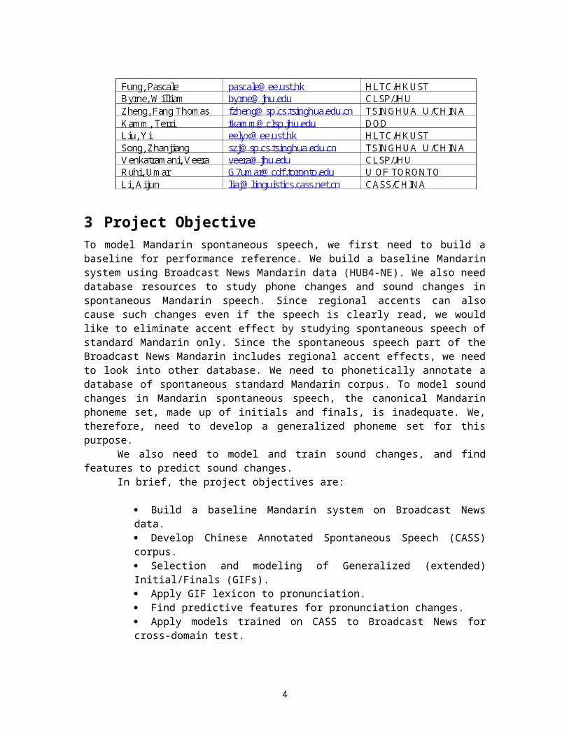
2 ParticipantsThe participants of this group include researchers and graduate students from China, Hong Kong and North America. Many of the participants have previous experience in either modeling English spontaneous speech or Mandarin spontaneous speech. One consultant to the group is Professor Li from the Chinese Academy of Social Sciences who led the annotation effort of the CASS corpus [1].

3 Project ObjectiveTo model Mandarin spontaneous speech, we first need to build a baseline for performance reference. We build a baseline Mandarin system using Broadcast News Mandarin data (HUB4-NE). We also need database resources to study phone changes and sound changes in spontaneous Mandarin speech. Since regional accents can also cause such changes even if the speech is clearly read, we would like to eliminate accent effect by studying spontaneous speech of standard Mandarin only. Since the spontaneous speech part of the Broadcast News Mandarin includes regional accent effects, we need to look into other database. We need to phonetically annotate a database of spontaneous standard Mandarin corpus. To model sound changes in Mandarin spontaneous speech, the canonical Mandarin phoneme set, made up of initials and finals, is inadequate. We, therefore, need to develop a generalized phoneme set for this purpose.

We also need to model and train sound changes, and find features to predict sound changes.

In brief, the project objectives are:

Build a baseline Mandarin system on Broadcast News data. Develop Chinese Annotated Spontaneous Speech (CASS) corpus. Selection and modeling of Generalized (extended) Initial/Finals (GIFs). Apply GIF lexicon to pronunciation. Find predictive features for pronunciation changes. Apply models trained on CASS to Broadcast News for cross-domain test.

4 AchievementOver the course of six weeks, we have successfully achieved the following:

Everything worked with respect to baseline. We have developed the Chinese Annotated Spontaneous Speech (CASS) Corpus. We have extended the canonical Mandarin Initial/Final set into Generalized Initial/Finals (GIFs) by selecting and refining some of the sound changes into GIF classes.

3

We discovered that direct acoustic feature that can be used without a pronunciation dictionary, framework established for incorporating direct measures into pronunciation models. We implemented a flexible Dynamic Programming (DP) alignment tool with cost functions for phone or phone class alignment. This tool will be made publicly available. We developed reasonable ways to derive phonetic variability from the CASS, and train them under sparse data condition. We have also applied pronunciation models from the CASS corpus to the Broadcast News corpus for cross-domain pronunciation modeling.

In the following sections, we will first give an overview of previous work in Mandarin pronunciation modeling, and some methods in English pronunciation modeling including state-level Gaussian sharing and decision tree derivation. We will then give an introduction of the CASS corpus in section 6.2, and the extended GIF set in section 6.3. The selection and refinement of the GIF set will be given next. Training sound changes in Mandarin speech in the sparse data condition is described in section 7. A description of the baseline Broadcast News Mandarin system is given in section 8.4. Decision-tree based pronunciation modeling of the Broadcast News data is described in section 8. We then conclude in the final section.

5 Previous WorkThere have been many attempts to model pronunciation variation including forced alignment between base form and surface form phonetic strings [2], shared Gaussians for allophonic modeling [3], as well as decision trees [4].

Modeling pronunciation variation in spontaneous speech is very important for improving the recognition accuracy. One limitation of current recognition systems is that their dictionaries for recognition only contain one standard pronunciation for each entry, so that the amount of variability that can be modeled is very limited. Previous work by Liu and Fung [5] proposed generating pronunciation networks based on rules instead of using a traditional dictionary for the decoder. The pronunciation networks consider the special structure of Chinese and incorporate acceptable variants for each syllable in Mandarin. Also, an automatic learning algorithm is designed to get learn the variation rules from data. The proposed method was applied to the Hub4NE 1997 Mandarin Broadcast News Corpus using the HLTC stack decoder. The syllable recognition error rate was reduced by 3.20% absolutely when both intra- and inter-syllable variations are both modeled.

Another approach by Liu and Fung [6] focuses on the characteristics of Mandarin Chinese. Chinese is monosyllabic and has simple syllable structure, which make pronunciation variation in spontaneous Mandarin speech abundant and difficult to model. Liu and Fung proposed two methods to model pronunciation variations in spontaneous Mandarin speech. First, a DP alignment algorithm was used to compare canonical and observed pronunciations and from that relation a probability lexicon was generated to model intra-syllable variations. Second, they propose integrating variation probability into the decoder to model inter-syllable variations. Experimental results show that by applying the probability lexicon the WER decreased by 1.4%. After incorporating variation probabilities into the decoder, WER significantly decreased by 7.6% compared to the baseline system.

Saraclar et al. [3] proposed to model pronunciation variability by sharing Gaussian densities across phonetic models. They showed that conversational speech exhibits considerable pronunciation variability. They pointed out that simply improving the accuracy of the phonetic transcription used for acoustic model training is of little benefit, and acoustic models trained on the most accurate phonetic transcriptions result in worse recognition than acoustic models trained on canonical base forms. They suggested that, “rather than allowing a phoneme in the canonical

4

pronunciation to be realized as one of a few distinct alternate phones, the hidden Markov model (HMM) states of the phoneme’s model are instead allowed to share Gaussian mixture components with the HMM states of the models of the alternate realizations”.

Saraclar et al. propose a state-level pronunciation model (SLPM), where the acoustic model of a phoneme has the canonical and alternate realizations represented by different sets of mixture components in one set of HMM states. The SLPM method, when applied to the Switchboard corpus, yielded a 1.7% absolute improvement, showing that this method is particularly well suited for acoustic model training for spontaneous speech.

Decision-tree based pronunciation modeling methodology has proven effective for English read speech and conversational speech recognition [4, 7]. This approach casts pronunciation modeling as a prediction problem where the goal is to predict the variation in the surface form pronunciation, as phonetically transcribed by expert transcribers) given the canonical (i.e. base form) pronunciation, derived from a pronunciation lexicon and a word transcription.

One of the major goals of this project is to apply these techniques, which were developed on English, to Mandarin.

5

6 Pronunciation Modeling in CASS

6.1 GENERALIZED INITIAL FINAL MODELING BASED ON CASS CORPUS When people speak casually in daily life, they are not consistent in their pronunciation. When we listen to such casual speech, it is quite common to find many different pronunciations of individual words. Current automatic speech recognition systems can reach word accuracies above 90% when being evaluated on carefully produced standard speech, but in recognizing casual, unplanned speech, its performance drops greatly. There are many reasons for this. In casual speech, phone change and sound change phenomena are common. There are often sound or phone deletions and/or insertions. These problems are made especially severe in Mandarin casual speech since most Chinese are non-native Mandarin speakers. Chinese languages such as Cantonese are as different from the standard Mandarin as French is different from English. As a result, there is an even larger pronunciation variation due to the influence of speakers' native language.

To find a solution to this problem in acoustic modeling stage, a speech recognition unit (SRU) set should be well defined so that it can well describe the phone/sound changes, including insertions and deletions. An annotated spontaneous speech corpus should also be available, which at least has the base form (canonical) and surface form (actual) strings of SRUs.

The Chinese Annotated Spontaneous Speech (CASS) corpus will be introduced in Section 6.2. Based on the transcription and statistics of CASS corpus, the generalized initials/finals (GIFs) is proposed to be the SRUs in Section 6.3. In Section 6.4, we construct the framework for the pronunciation modeling, where an adaptation method is used for the refined acoustic modeling and a context-dependent weighting method is used to estimate the output probability of any surface form given its corresponding base form. Section 6.5 lists the experimental results while summaries and conclusions are given in Section 6.6.

6.2 CASS CorpusA Chinese Annotated Spontaneous Speech (CASS) corpus was created to collect samples of most of the phonetic variations in Mandarin spontaneous speech due to pronunciation effects, including allophonic changes, phoneme reduction, phoneme deletion and insertion, as well as duration changes.

Made in ordinary classrooms, amphitheaters, or school studios without the benefit of high quality tape recorders or microphones, the recordings are of university lectures by professors and invited speakers, student colloquia, and other public meetings. The collection consists primarily of impromptu addresses, and were delivered in an informal style without prompts or written aids. As a result the recordings are of uneven quality and contain significant background noises. The recordings were delivered in audiocassettes and digitized into single-channel audio files at 16kHz rate and with 16-bit precision. A subset of over 3 hours’ speech was chosen for detailed annotation, which formed the CASS corpus. This corpus contains the utterances of 7 speakers at a speed as fast as about 4.57 syllables per second on an average, and in standard Chinese with slight dialectal backgrounds.

The CASS corpus was transcribed into a five-level annotation. Character Level. Canonical sentences (known as word/character sequences) are

transcribed. Toned Pinyin (or Syllable) Level. A segmentation program was run to convert the

character level transcription into word sequences, and then the word sequences were changed into sequences of toned pinyins through a standard word-to-pinyin lookup dictionary. After carefully checked, the canonical toned pinyin transcription was generated.

6

Initial/Final Level. This semi-syllable level’s transcription only includes the time boundaries for each (observed) surface form initial/final.

SAMPA-C Level. This level contains the observed pronunciation in SAMPA-C [8, 9], which is a labeling set of machine-readable International Phonetic Alphabet (IPA) symbols adapted for Chinese languages from the Speech Assessment Methods Phonetic Alphabet (SAMPA). In SAMPA-C, there are 23 phonologic consonants, 9 phonologic vowels and 10 kinds of sound change marks (nasalization, centralization, voiced, voiceless, rounding, syllabic, pharyngrealization, aspiration, insertion, and deletion), by which 21 initials, 38 finals, 38 retroflexed finals as well as their corresponding sound variability forms can be represented. Tones after tone sandhi, or tonal variation, are attached to the finals.

Miscellaneous Level. Several labels related to spontaneous phenomenon are used to independently annotate the spoken discourse phenomena, including modal/exclamation, noise, silence, murmur/unclear, lengthening, breathing, disfluency, coughing, laughing, lip smack, crying, non-Chinese, and uncertain segments. Information in this level can be used for garbage/filler modeling.

6.3 Generalized Initials/FinalsIn spontaneous speech, there are two kinds of differences between the canonical initials/finals (IFs) and their surface forms if the deletion and insertion are not considered. One is the sound change from one IF to a SAMPA-C sequence close to its canonical IF, such as nasalization, centeralization, voiceless, voiced, rounding, syllabic, pharyngealization, and aspiration. We refer to the surface form of an IF as its generalized IF (GIF). Obviously, the IFs are special GIFs. The other is the phone change directly from one IF to another quite different IF or GIF, for example, initial /zh/ may be changed into /z/ or voiced /z/.

If we want to model the sound variability in our acoustic modeling and we choose semi-syllable level units as SRUs, the first thing to do is to choose and define the GIF set.

6.3.1 Definition of GIF Set

The canonical IF set consists of 21 initials and 38 finals, totally 59 IFs. By searching in the CASS corpus, we initially obtain a GIF set containing over 140 possible SAMPA-C sequences (pronunciations) of IFs; two examples are given in Table 1. However, some of them occur for only a couple of times which can be regarded as least frequently observed sound variability forms therefore they are merged into the most similar canonical IFs. Finally we have 86 GIFs.

Table 1: Examples for IFs and their possible pronunciations in SAMPA-C format.

7

These well-chosen GIFs are taken as SRUs. In order to well model the spontaneous speech, additional garbage models are also built for breathing, coughing, crying, disfluency, laughing, lengthening, modal, murmur, non-Chinese, smacking, noise, and silence.

6.3.2 Probabilistic GIFs

Once the GIF set is determined, a GIF-set-specific GIF Level transcription should be made according to the SAMPA-C Level transcription. We call this kind of transcription a dynamic transcription in comparison with the original five levels’ transcriptions. Dynamic transcriptions are useful in the training and testing procedures.

From the statistics of the dynamic GIF transcription, the GIF output and transition probabilities are estimated for later use. The GIF output probability is defined as the probability of a GIF given its corresponding IF, written as P (GIF | IF). To include the GIF deletion, P (<Del> | IF) will also be estimated.

The GIF N-Grams, including unigram P(GIF), bigram P(GIF2 | GIF1) and trigram P(GIF3|GIF1,GIF2), give the GIF transition probabilities.

6.3.3 Generalized Syllable (GS)

Similar to generalized initials/finals, we refer to any possible pronunciation of a given canonical syllable as one of its generalized syllables (GSs). According to the CASS corpus as well as the dynamic GIF transcription, it is easy to find all possible GSs. Table 2 is an example, where syllable ‘chang’ corresponds to 8 possible pronunciations, or generalized syllables, each of which has an output probability P ([GIF1] GIF2 | Syllable), defined as the probability of the GIF sequence (one generalized initial followed by one generalized final) given its corresponding canonical syllable and can be learned from the CASS corpus. This gives a probabilistic multi-entry syllable-to-GIF lexicon

Table 2: A standard Chinese syllable and its possible pronunciations in SAMPA-C with output probability.

6.4 PRONUNCIATION MODELINGGiven an acoustic signal of spontaneous speech, the goal of the recognizer is to find the canonical/baseform syllable string that maximize the probability P(B|A). According to the Bayes’ Rule, the recognition result is

8

In Equation , is the acoustic modeling part and is the language modeling part. In this section we first focus only on the acoustic modeling and propose some approaches to the pronunciation modeling.

6.4.1 Theory

Assume is a string of canonical syllables, i.e., . For simplification, we apply the independence assumption to the acoustic probability,

where is the partial acoustic signal corresponding to syllable . In general, by developing any term in right hand of Equation we have

where s is any surface form of syllable b, in other words, s is any generalized syllable of b. Therefore, the acoustic model is divided into two parts, the first part is the refined acoustic model while the second part is the conditional probability of generalized syllable s. Equation provides a solution to the sound variability modeling by introducing a surface form term. In the following subsections, we will present methods for these two parts.

6.4.2 IF-GIF Modeling

According to the characteristics of Chinese language, any syllable consists of an initial and a final. Because our speech recognizer is designed to take semi-syllables as SRUs, term should be rewritten in terms of semi-syllables. Assume and , where and are the canonical initial and the generalized initial respectively, while and are the canonical final and the generalized final respectively. Accordingly, the independence assumption results in

More generally, the key point of the acoustic modeling is how to model the IF and GIF related semi-syllable, i.e., how to estimate . There are three different choices:

Use to approximate . This is the acoustic modeling based on IFs, named as the independent IF modeling. Use to approximate . Based on [3, 10], this is the acoustic modeling based on GIFs, referred to as the independent GIF modeling. Estimate . This can be regarded as a refined acoustic modeling taking both the base form and the surface form of the SRU into consideration. Thus we refer it to as the IF-GIF modeling.

It is obvious that the IF-GIF modeling is the best choice among these three kinds of modeling methods if there are sufficient training data. This kind of modeling method needs a dynamic IF-GIF transcription.

The IF Transcription is directly obtained from the Syllable Level transcription via a simple syllable-to-IF dictionary, and this transcription is canonical. The GIF transcription is obtained by means of the method described in Section 6.3.2 once the GIF set is determined. By comparing the IF and GIF transcriptions, an actual observed IF transcription, named as IF-a transcription, is generated, where the IFs corresponding to deleted GIFs are removed and the IFs corresponding to the inserted GIFs are inserted. Finally the IF-GIF transcription is generated directly from the IF-a and GIF transcriptions. Table 3 is an example to illustrate how the IF-GIF

9

transcription is obtained. However, if the training data are not sufficient, the IF-GIF modeling will not work well or even work worse due to the data sparseness issue.

Table 3: The way to generate IF-GIF transcription.

Figure 1: B-GIF modeling: adapting P(a|b) to P(a|b,s). Initial IF-GIF models cloned from the associated IF model. In this example, base form IF has three surface forms GIF1, GIF2, and GIF3. Given model IF, we generate three initial IF-GIF models, namely IF-GIF1, IF-GIF2, and IF-GIF3.

A reasonable method is to generate the IF-GIF models from their associated models; the adaptation techniques described in [11] can be used. There are at least two approaches. The IF-GIF models can be transformed either from the IF models or from the GIF models. The former method is called the base form GIF (B-GIF) modeling and the later the surface form GIF (S-GIF) modeling.

The procedure for generating IF-GIF models using B-GIF method is:Step 1. Train all IF models according to the IF-a transcription.Step 2. For each , generate the initial IF-GIF models by copying from model according to its corresponding GIFs . The resulting IF-GIF models include

. This procedure is illustrated in Figure 1.Step 3. Adapt the IF-GIF models using the corresponding IF-GIF transcription. We use the term ‘adaptation’ just for simplification; it is different from its original meaning.

10

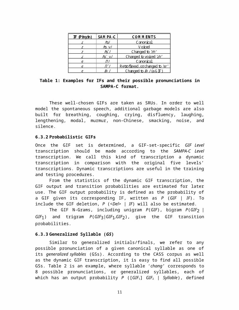
Figure 2: S-GIF modeling: adapting P(a|s) to P(a|b,s). Initial IF-GIF models cloned from the associated GIF model. In this example, three base forms IF1, IF2 and IF3 share the same surface form GIF. Given model GIF, we generate three initial IF-GIF models, namely IF1-GIF, IF2-GIF and IF3-GIF.

The procedure for generating IF-GIF models using S-GIF method is:Step 1. Train all GIF models according to the GIF transcription.Step 2. For each , generate the initial IF-GIF models by copying from model according to its corresponding IFs . The resulting IF-GIF models include . This procedure is illustrated in Figure 2.Step 3. Adapt the IF-GIF models using the corresponding IF-GIF transcription, similarly to the B-GIF method.

The difference between S-GIF method and the B-GIF method lies only in how we generate the initial IF-GIF models; the former method copies from the base form models while the later one copies from the surface models. By comparing these two methods as illustrated in Figures 1 and 2, it is straightforward to conclude that the initial IF-GIF models using B-GIF method will have bigger within-model scatters than those using the S-GIF method. The analysis shows S-GIF method will outperform B-GIF method.

The IF-GIF modeling enables multi-entry for each canonical syllable. Considering the multi-pronunciation probabilistic syllable lexicon, each entry in HTK [11] has the form

where is the base form and is its surface form.

6.4.3 Context-Dependent Weighting

In Equation , the second part stands for the output probability of a surface form given its corresponding base form.

A simple way to estimate is to directly learn from the database with both base form and surface form transcriptions. The resulting probability is referred to as the Direct Output Probability (DOP).

The problem is that the DOP estimation will not be so accurate if the training database is not big enough. Actually, what we are considering in the pronunciation weighting are the

11

base form and surface form of Chinese syllables, and in the syllable level the data sparseness remains a problem, therefore many weights are often not well trained.

It is true that the syllable level data sparseness DOESN’T mean the semi-syllable (IF/GIF) level data sparseness, which suggests us to estimate the output probability via the semi-syllable statistics instead.

According to the Bayesian Rule, the semi-syllable level output probability of a surface form, i.e. a GIF, given its corresponding base form, i.e. an IF, can be rewritten according to the context information as

where is the context of IF, it can be a bigram, a trigram or whatever related to this IF. Supposing includes the current and its left context , Equation can be rewritten as

In the sum on the right hand side of Equation , term is the output probability given the context and term is similar to the IF transition probability. These two terms can be learnt from the database directly; hence Equation is easy to be calculated offline. Based on the way of developing the output probability , this method is called Context-Dependent Weighting (CDW) and the estimated probability is called the Context-Dependent Weight (CDW). If we define

,

Equation can be rewritten as

,

and according to Equation , we define another function:

The above equations are focused on the initial and final, and the IF pair could be either a (initial, final) pair or a (final, initial) pair.

To give the syllable level output probability estimation as in Equation , we have three different methods:

CDW-M:

CDW-P:

CDW-Q:

where and as in Section 4.2. Obviously Equation considers the inner-syllable constrains, which is believed to be more useful. If Equation or Equation is used, the sum of approximated over all possible s for b is often less than 1.0 and will often not be 1.0, that’s the reason we call it the weight instead of the probability.

If we do not consider the IF-GIF modeling, instead we assume that in Equation , in other words the acoustic modeling is exactly the GIF modeling. In this case

12

the use of the CDW results in that the multi-pronunciation probabilistic syllable lexicon will have entries in the form of

where the weight can be taken as one from Equations , , or . Nothing taken for means the equal probability or weight.

6.4.4 Integrating IF-GIF modeling and Context-Dependent Weighting

When we consider both the CDW and the IF-GIF modeling, we will combine Equations and together and have the multi-pronunciation syllable lexicon with entry in the form of

6.5 Experimental ResultsAll experiments are done using the CASS corpus. The CASS corpus is divided into two

parts, the first part is the training set with about 3.0 hours spontaneous speech data and the second is the testing set with about 15 minutes spontaneous speech data. The HTK is used for the training, adaptation and testing [11]. A 3-state 16-gaussian HMM is used to model each IF, GIF or IF-GIF. The feature used here is 39-dimension MFCC_E_D_A_Z. The feature extraction frame size is 25 ms with 15 ms overlapped between any two adjacent frames.

Experimental results include (1) UO: unit (IF, GIF or IF-GIF) level comparison without the syllable lexicon constraint; (2) UL: unit level comparison with the syllable lexicon constraint; and (3) SL: syllable level comparison with the syllable lexicon constraint. The listed percentages are

correctness percentage:

accuracy:

deletion percentage:

substitution percentage:

and insertion percentage : .

where Num is the total number of SRUs tested, and Hit, Del, Sub and Ins indicate numbers of hit, deletion, substitution and insertion respectively.Experiment 1. Independent IF modeling. The first experiment is done to test the canonical IF modeling and the result is listed in Table 4: IF Modeling Result.. The lexicon used here is a single-entry syllable-to-IF lexicon with equal weight, because each syllable corresponds to a unique canonical initial and a unique canonical final. This is just for comparison.

Table 4: IF Modeling Result.

13

Experiment 2. Independent GIF modeling. This is the baseline system where an equal probability or weight is provided for the multi-entry syllable-to-GIF lexicon. Experimental result is shown in Table 5. By comparing the two tables, we find that in general the performance of independent GIF modeling is worse than independent IF modeling if no more pronunciation method is adopted. It is obvious, because the GIF set is bigger than the IF set , which results in that GIFs are not better trained than IFs on the same training database.

Table 5: Baseline: Independent GIF Modeling Result.

Experiment 3. IF-GIF Modeling. This experiment is designed to test the IF-GIF modeling, . Except the acoustic models themselves, the experiment condition is similar to that in

Experiment 2. The B-GIF and S-GIF modeling results are given in Table 6 and Table 7 respectively. We have tried the mean updating, MAP adaptation and MLLR adaptation methods for both B-GIF and S-GIF modeling, and listed are the best results.

From the two tables, it is seen that S-GIF outperforms B-GIF; the reason can be found in Figure 1 and Figure 2 and is explained in Section 6.4.2. Compared with the GIF modeling, the S-GIF modeling achieves a syllable error rate (SER) reduction of 3.6%.

Table 6: B-GIF Modeling Result.

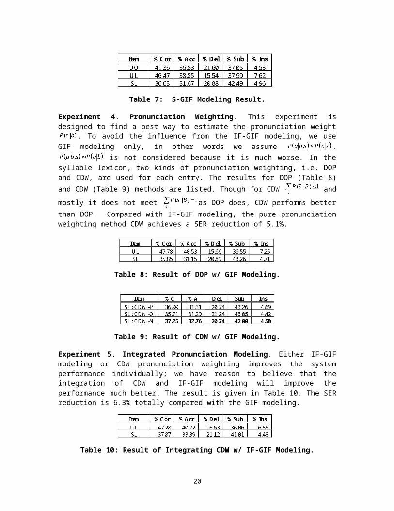
Table 7: S-GIF Modeling Result.

Experiment 4. Pronunciation Weighting. This experiment is designed to find a best way to estimate the pronunciation weight . To avoid the influence from the IF-GIF modeling, we use GIF modeling only, in other words we assume . is not considered because it is much worse. In the syllable lexicon, two kinds of pronunciation weighting, i.e. DOP and CDW, are used for each entry. The results for DOP (Table 8) and CDW (Table 9) methods are listed. Though for CDW and mostly it does not meet

as DOP does, CDW performs better than DOP. Compared with IF-GIF modeling, the pure pronunciation weighting method CDW achieves a SER reduction of 5.1%.

14

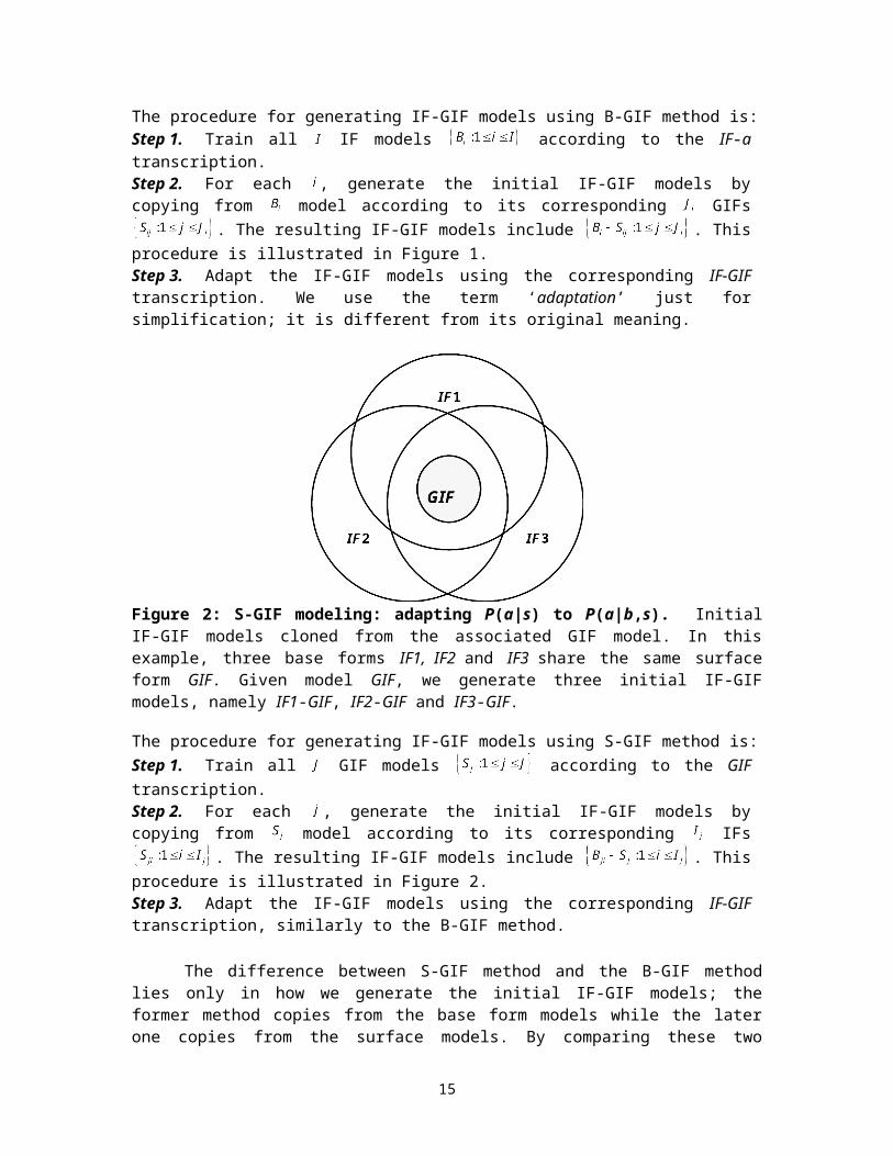
Table 8: Result of DOP w/ GIF Modeling.

Table 9: Result of CDW w/ GIF Modeling.

Experiment 5. Integrated Pronunciation Modeling. Either IF-GIF modeling or CDW pronunciation weighting improves the system performance individually; we have reason to believe that the integration of CDW and IF-GIF modeling will improve the performance much better. The result is given in Table 10. The SER reduction is 6.3% totally compared with the GIF modeling.

Table 10: Result of Integrating CDW w/ IF-GIF Modeling.

Experiment 6. Integration of syllable N-gram. Though language modeling is not the focus of pronunciation modeling, to make Equation a complete one, we borrow a cross-domain syllable language model. This syllable bigram is trained using both read texts from Broadcast News (BN) and spontaneous texts from CASS, the amount of texts from BN is much bigger than those from CASS, and therefore we call it a borrowed cross-domain syllable bigram. From the result listed in Table 11, it is not difficult to conclude that this borrowed cross-domain syllable N-gram is helpful. The SER reduction is 10.7%.

Table 11: Result of Integrating the Syllable N-gram.

Figure 3 gives an outline of all above experimental results. The overall SER reduction compared with GIF modeling and IF modeling is 6.3% and 4.2% (all without syllable N-gram).

15

Figure 3: A summary of experimental results.

6.6 Discussion In order to model the pronunciation variability in spontaneous speech, firstly we propose the concept of generalized initial/final (GIF) and generalized syllable (GS) with or without probability, secondly we propose the GIF modeling and IF-GIF modeling aiming at refining the acoustic models, thirdly we propose the context-dependent weighting method to estimate the pronunciation weights, and finally we integrate the cross-domain syllable N-gram into the whole system.

Although the introduction of the IF-GIF modeling and the pronunciation weighting leads to performance reduction on the unit level compared with the IF modeling, but the syllable level overall performance for IF-GIF modeling greatly outperforms the IF modeling. From the experimental results, we conclude that

The overall GIF modeling is better that the IF modeling. By refining the IF and GIF, the resulting IF-GIF modeling is better than both the IF modeling and the GIF modeling , even if data is sparse, when the S-GIF/B-GIF adaptation techniques can be used to provide a solution to data sparseness. The S-GIF method outperforms the B-GIF method because of the well-chosen adaptation initial models. The context-dependent weighting (CDW) is more helpful for sparse data than direct output probability (DOP) estimating. The cross-domain syllable N-Gram is useful.

In summary, our ongoing work includes: Generating a bigger corpus with both IF and GIF transcriptions, Investigating phone and sound changes in Mandarin with accent(s), Applying state-level Gaussian sharing to IF-GIF models and using context-dependent modeling, and Training a more accurate N-gram model using a bigger text corpus of either spontaneous speech or cross-domain speech.

These points are expected to be helpful in automatic spontaneous speech recognition.

16

7 Pronunciation Modeling with Sparse DataIn the CASS data, we found that there are not many phone changes from one canonical phone to another. This is possibly due to syllabic pronunciation nature in Mandarin though this hypothesis needs to be verified by psycholinguistic studies. On the other hand, there are more sound changes or diacritics (retroflex, voiced) in the database. One obvious approach is to extend the phoneme set to GIFs as described in Section 6. As described, we need to train these extended models from annotated data since the sound changes do not exist in canonical pronunciation lexicons and thus we need to annotate the training data with such sound changes.

One problem that we have to tackle is the sparseness of such annotated sound change samples. Phoneme models built on sparse data are not reliable. We propose two methods to solve this sparse data problem—(1) state-based Gaussian sharing between phoneme models; and (2) deleted interpolation between the canonical IF set and the extended GIF set.

7.1 Flexible Alignment ToolsIn pronunciation modeling, one important step is the alignment of the base canonical form to the surface form phoneme strings. This alignment is commonly done by dynamic programming (DP) using edit distance as cost function. However, simple string edit distance is inadequate. For example, given the base-form and surface form utterances such as:

Baseform: n ei c i z ai zhSurfaceform: n ai i c i a zh

Since the string length for both utterances is the same, the symbols align one to one and the cost between the two utterance is the sum of substitution costs between each symbol.

However what is most likely to have happened is the following: /ei/ was heard as /ai/, /i/ was inserted, /z/ was deleted, /ai/ was heard as /a/, giving the following alignment:

Baseform: n ei - c i z ai zhSurfaceform: n ai i c i - a zh

To make use of this information, we implement a flexible alignment tool that uses a DP alignment technique but incorporates inter-symbol comparison costs and rules. The alignment can also be done between phonetic classes in addition to individual phones.

We use the FSM Toolkit available from AT&T labs [12] to generate DP alignments between base and surface form utterances. The tools designed for the project will be made publicly available as open-source and, as mentioned earlier, they can be adapted for other languages and domains.

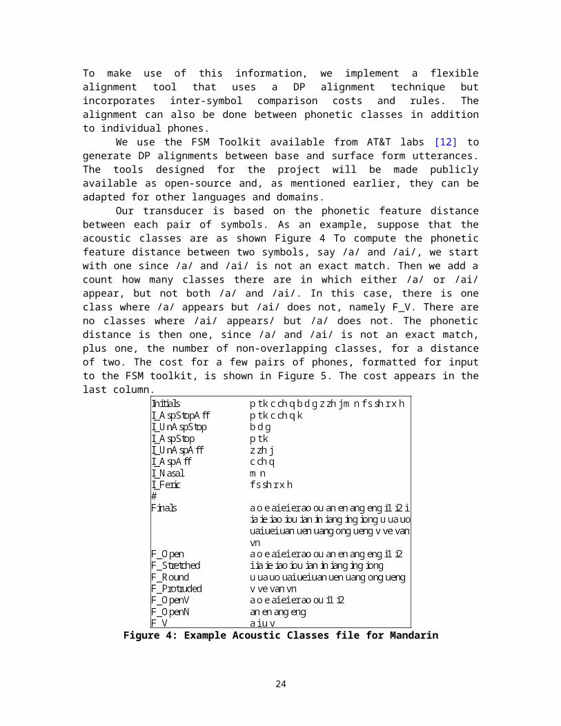
Our transducer is based on the phonetic feature distance between each pair of symbols. As an example, suppose that the acoustic classes are as shown Figure 4 To compute the phonetic feature distance between two symbols, say /a/ and /ai/, we start with one since /a/ and /ai/ is not an exact match. Then we add a count how many classes there are in which either /a/ or /ai/ appear, but not both /a/ and /ai/. In this case, there is one class where /a/ appears but /ai/ does not, namely F_V. There are no classes where /ai/ appears/ but /a/ does not. The phonetic distance is then one, since /a/ and /ai/ is not an exact match, plus one, the number of non-overlapping classes, for a distance of two. The cost for a few pairs of phones, formatted for input to the FSM toolkit, is shown in Figure 5. The cost appears in the last column.

17

Figure 4: Example Acoustic Classes file for Mandarin

Figure 5: Cost Transducer for Example Acoustic Classes

18

Figure 6: Example Showing Alignment of 4 Tiers

The Aligner can be used for multiple-tier alignment. An example of a 4-tier alignment is shown in Figure 6. In this case, we added rules to enhance the inter-symbol costs:

rules based upon diacritics information (e.g. voicing information) rules for insertion and deletion of different symbols (e.g. in Mandarin, initials

tend to get deleted more easily) rules listing additional symbols for garbage models rules for merging two or more symbols into one (e.g. when an initial and a final

are combined to make a single symbol)Details about the additional rules can be obtained by downloading the Flexible Alignment

Tool from http://www.clsp.jhu.edu/ws2000/groups/mcs/Tools/README.html.

7.2 STATE-LEVEL SHARED GAUSSIAN MIXTURESPronunciations in spontaneous, conversational speech tend to be much more variable than in careful read speech. Most speech recognition systems rely on pronunciation lexicons that contain few alternative pronunciations for most words. Most state-of-the-art ASR systems estimate acoustic models under the assumption that words in the training corpus are pronounced in their canonical form [3]. As far as we know, most of the research work in pronunciation modeling is focused on lexicon level, adding alternative phoneme strings to represent pronunciations for each lexical entry. This is perhaps the easiest way to incorporate some pronunciation information as human can read out the words aloud and write down the phoneme transcription accordingly. Of course, as we described in [6], and as Saraclar et al [3] showed, merely adding more phoneme strings causes more confusion to the speech recognizer and thus a probabilistic pronunciation lexicon is proposed in [5, 6] where the actual probability of a phoneme given canonical phoneme and the context-dependent phoneme transitions are extracted from recognition confusion matrix. This probabilistic lexicon is effective in improving word accuracies.

The assumption above is that there are entire phone changes in the alternative pronunciation, represented by a distinctive phoneme string. Such discrete changes are of course, far from reality. In the CASS database, we found that there are more sound changes than phone changes in casual Mandarin speech. Such sound changes are deviations from canonical phoneme models to various degrees, at various stages of the phoneme onset, stationary state and transition to the next phoneme. In order to model such changes, we propose state-level Gaussian mixture sharing between initial/final (IF) models aligned by variable-cost dynamic programming (DP). Previous work by Saraclar et al. [3] uses decision-tree clustering of the shared phonemes.

19

Decision tree is useful for clustering phoneme classes, based on the fact that most English pronunciation variations come from phone changes. In our work this summer, we studied the HMM state level pronunciation variations with a cost matrix between different phone state levels as weights for sharing. Such cost matrix is obtained by DP alignment, with variable costs associated with different phoneme replacement, insertion, and deletion. As described in the previous section, this cost matrix is more refined and accurate than traditional binary DP alignment method. With the variation probabilities of each phoneme state, we share Gaussian mixtures among the canonical and its alternate realizations. Compared to the decision-tree approach, our approach is applicable to both phone changes and sound changes. For example, rather than adding alternate phones for phoneme /p/ such as /p_v/ or /p_h/, the HMM states of phoneme /p/ are shared with the Gaussian mixtures of the PDF of /p_v/ and /p_h/. This means that the acoustic model of phoneme p includes the canonical and its corresponding alternate realizations (represented by different sets of mixture components in one set of HMM states) according to variation probabilities.

7.2.1 Algorithm

The basic steps for state level pronunciation model are as follows:

1. Align base form and surface form in state level.2. Count the relative frequency between phonemes and phones.3. Estimate variation probabilities with count numbers and cost matrix between phonemes

and phones.4. Share phone’s PDF of each state to phoneme’s corresponding phone states with variation

probabilities.5. Re-estimate shared Gaussian mixture HMM models.

Details of the above steps are showed as follows:1) Alignment

1. With canonical phonemic transcriptions of the training utterances, do forced alignment with canonical one-to-one mapping syllable to phoneme lexicon, obtain state-level base form transcription.

2. Get the surface form state-level transcription with recognizer.3. Use DP method, with phoneme to phone state-level cost matrix, do state-to-state

alignment between base form and surface form state-level transcriptions.1) Counting

Use the state level alignment results, calculate the relative frequency of state bin the base form sequence when it is DP aligned with state s in the surface form sequence. The pronunciation variation probability is written as

2) Calculate variation probabilityConsider the cost matrix between phoneme and phones, equation should be:

20

is constant, is the cost value between the base form state and the surface form state . Conventional approaches only consider a uniform cost for alignment between a state in the surface form to another state . In practice, this is not accurate. For example: base form state p[3] is aligned with different surface form state p_v[3], d[3] and p_v[1], the cost matrix will give us: (the smaller the value, the more similar the states)

According to equation , the variation probability is different and p[3] to p_v[3] gives the highest similarity value. We then select the top N list for each , by representing the most similar phone states as

,

and then doing normalization of ,

One example of state variation probabilities is shown in Table 12.

Table 12: State-level variation probabilities

3) Gaussian mixtures are shared with as follows: 1. Suppose the original output distribution of state is

.

2. Share the PDFs of the surface form state to its corresponding base form state , combined the normalized to the original mixture weights.

3. The shared mixtures PDF is:

4) Baum-Welch algorithm is used for further re-training the shared mixtures HMM models.

21

7.2.2 Experimental results

The experiments are performed on both CASS and BN database. In the CASS database, the Gaussian mixtures are shared between IF and GIF models. In the BN database, the mixtures are shared between different IF models.

7.2.2.1 In CASS databaseInitial/Final HMM Units

For IF models, the total number of IF units is 63, we also add some special symbols for modeling crying, laughing and other phenomena in spontaneous speech, so that the total number of units used in the system is 70. The other experiment conditions are the same as section 7.1, training data for training pronunciation model is 3060 utterances with 7 different speakers, all the speech are spontaneous Mandarin speech.

Table 13: IF Unit Performance of BaseLine and Shared Gaussian Mixtures between IFs

GIF HMM UnitsFor GIF models, the total number of GIF units is 90, we also add the extended GIF

symbols. The experimental condition is the same as for the IF model. The lexicon used in the recognition is multi-pronunciation syllable to GIF lexicon.

Table 14: GIF Unit Performance of BaseLine and Shared Gaussian Mixtures between IF and GIF

We found that the syllable accuracy improved by 0.65% absolute percentage. In the three hours data, we found that some alternate realizations of phonemes seldom occur in the surface form. Given the limited sound change training data, this is a very encouraging result. Consequently, we try to apply the same method with context-dependent initials to the BN database as described in the next section.

7.2.2.2 In Broadcast News databaseIn the BN database, context-depend initials and context-independent finals are selected as

the HMM unit. The total number of CD_initial and CI_final is 139. The training data for acoustic modeling and pronunciation modeling is about 10 hours with over 10,000 utterances. The testing data includes spontaneous speech, conversational speech, broadcast news speech, etc. The speech in BN database with high background noise is not used for training and testing. The testing data is 724 utterances. We use 32 Gaussian mixtures.

22

Table 15: Performance of Baseline and Shared Gaussian Mixtures in BN database

From the experiments we found that the recognition accuracy improved significantly by 6.54% absolute after 8 iterations re-train the shared models. Compared to the experiment results in CASS database, share Gaussian mixture method is more effective for the BN database. We believe that this is because there is more data samples for pronunciation model training and context-dependent initial models are also more effective than context-independent initial models.

7.3 DELETED INTERPOLATIONDeleted interpolation is regarded as one of the most powerful smoothing techniques to improve the performance of acoustic models as well as language models in speech recognition [13]. It is often necessary to combine well-trained general models with less well-trained but more refined models [14, 15].

In the three-hour CASS database, we found that there is a limited number of training samples for the GIF set. We thus propose using deleted interpolation together with state-level Gaussian sharing at each iteration step to improve the GIF models.

The total number of GIF models is 90 and the total number of canonical IFs is 63. GIF is an extended set of IF models and include the latter. Some of the similar GIF models are combined into equivalent classes, for example: “a_6_h” and “a_h_u” are merged. The number of GIF models needing deleted interpolation is 20, some examples are as follows:

A general deleted interpolation equation is:

In our work, the GIF models are regarded as more detailed but less well trained models whereas IF models are less refined but well trained. The interpolation weights are estimated using cross-validation data with the EM algorithm. In our experiments, we only focus on continuous HMMs.

23

7.3.1 Deleted Interpolation of IF/GIF Models

For HMM with continuous PDFs, the interpolated PDF can be written in terms of a more detailed but less well trained PDF and a less detailed but better trained PDF . Equation becomes as follows:

is the mixture function after deleted interpolation for GIF HMM model , is the related IF mixture, is the interpolation weight for each .

For cross validation, the training data for obtain interpolation weight is divided into parts and a set of and is trained from each combination of parts, with

the deleted part serving as the unseen data to estimate a set of interpolation weights .

7.3.2 Algorithm

Next steps illustrate how to estimate the interpolation weights , is the HMM model. Initialize with arbitrary value, , set threshold to a small value. Divide the training data into sets. Train and model from each combination of parts with EM algorithm, the residual part is reserved as the deleted part for cross-validation. From step 2, we obtained and . is the PDF of GIF model trained by the whole training data except part (deleted part). Similarly is the PDF of the related IF trained by the same part. Perform phone recognition on the deleted part using the models. Aligning the phoneme recognition results with base form transcriptions, we obtain , the number of data points in part that have been aligned with GIF model . From aligned results, find the data-point in input MFCC files, is the deleted part , is the k-th data point. Update by the following equation:

If , i.e. if the interpolation weight does not converge, go to Step 6,

use next aligned kth ; else go to Step 8. Stop.

7.3.3 PDF sharing with

Equation shows how is obtained from and with deleted interpolation weights. Suppose

24

is the mixture numbers and is the mixture weights of the density. Using interpolation weight , the interpolation density value for GIF model is:

7.3.4 Experimental results

CASS databaseIn CASS database, we already have hand-labeled GIF and IF transcriptions of training

and deleted part data. From left-to-right 5 states HMM models with 16 Gaussian mixtures were used. , the total number of utterances is 3092, as showed in step 3, training set includes 2061 utterances, deleted part includes 1031 utterances. We use back-off syllable bi-gram trained from BN database.

Table 16: Performance of GIF model in CASS with and without DI

25

8 Decision-tree Based Pronunciation ModelingIn acoustic modeling for speaker independent, large vocabulary speech recognition, the objective is to use speech from many speakers to estimate acoustic models that perform well when used to transcribe the speech of a new speaker. We have the same goal in using the CASS transcriptions for pronunciation modeling. The CASS corpus provides transcriptions of a relatively small collection of speakers recorded in somewhat unusual circumstances, and our goal is to use the CASS transcriptions to build statistical models which capture the regular pronunciation variations of Mandarin speakers in general.

We employ the decision-tree based pronunciation modeling methodology that has proven effective for English read speech and conversational speech recognition [4, 7]. This approach casts pronunciation modeling as a prediction problem. The goal is to predict the variations in the surface form (i.e. in the phonetic transcription provided by expert transcribers) given the baseform pronunciation derived from a pronunciation lexicon and a word transcription. The procedures that train these models identify consistent deviations from canonical pronunciation and estimate their frequency of occurrence. Given the relatively small amount of annotated data available for training it is not possible to obtain reliable estimates for all pronunciation phenomena: only events that occur often in the corpus can be modeled well. A conservative approach in this situation would model only those pronunciation changes observed often in the annotated data. A more ambitious approach which has proven effective would be to build large models using the annotated data, accept that they’re poorly estimated, and then refine them using additional, unlabeled data. This refinement process applies the initial models to the transcriptions of the acoustic training set, and an existing set of acoustic models is used to select likely pronunciation alternatives by forced alignment [4, 7]. The refinement effectively discards spurious pronunciations generated by the initial set of trees and also ’tunes’ the pronunciation models to the acoustic models that will be used in recognition.

In the pronunciation modeling work upon which this project is based [4, 7], phonetic annotations were available within the ASR task domain of interest. This allowed decision trees to be refined using speech and acoustic models from the same domain as the data used in building the initial models. Riley et al. [7], trained decision trees using the TIMIT read speech corpus [16] and then refined them using Wall Street Journal acoustic training data. In subsequent work, pronunciation models trained using phonetic transcriptions of a portion of the SWITCHBOARD conversational speech corpus [17] were refined using additional training data from the corpus [4]. While it would be ideal to always have annotated data within the domain of interest, it would be unfortunate if new phonetic transcriptions were required for all tasks. However, unlike acoustic models and language models, pronunciation lexicons have been proven to be effective across domains. This suggests that, apart from words and phrases that might be specific to particular task domains, it is reasonable to expect that pronunciation variability is also largely domain independent.

We take the optimistic view that an initial set of pronunciation models trained on the CASS SAMPA-C transcriptions will generalize well enough so that they contain pronunciation variability in the Mandarin Broadcast News domain. The model refinement will be used to identify which of the broad collection of alternatives inferred from the CASS domain actually occur in the Mandarin Broadcast News domain. After this refinement of the alternatives, new pronunciation lexicons and acoustic models will be derived for the Mandarin Broadcast News domain. In summary, we will take advantage of the refinement step to adapt CASS pronunciation models to a Broadcast News ASR system.

26

8.1 MANDARIN ACOUSTIC CLASSES FOR DECISION TREE PRONUNCIATION MODELS

Building decision trees for pronunciation models is an automatic procedure that infers generalizations about pronunciation variability. For instance, given the following two (hypothetical) examples of deletion of the Mandarin initial :

Pinyin Base Form Surface FormExample 1 bang fu b ang f u b ang uExample 2 ban fu b an f u b an u

we might hypothesize two rules about the deletion of the initial f

where “-” indicates deletion. Alternatively, we could hypothesize a single rule

that captures the two examples and also allows f to be omitted when preceded by a nasal and followed by a u as in “ben fu”. Decision tree training procedures choose between such choices based on the available training data. Ideally, equivalence classes will be chosen that balance specificity against generalization.

The use of acoustic classes for constructing decision trees for pronunciation modeling has been discussed at length in [4, 7, 18]. We adopt the approach as developed for English, although some alterations are needed in its application to Mandarin. In English the phonetic representation is by individual phones and acoustic classes can be obtained relatively simply from IPA tables, for instance. In Mandarin, the transcription is by initials and finals, which may consist of more than one phone. Because of this, the acoustic classes are not determined obviously from the acoustic features of any individual phone. The classes were constructed instead with respect to the most prominent features of the initials and finals. After consultation with Professor Li Aijun, the acoustic classes listed in Table 17-24 were chosen. Note that in these classes, indications of voicing are preserved, so that these classes can be applied to the CASS transcriptions.

8.2 NORMALIZATION AND ACOUSTIC ANNOTATION OF THE CASS TRANSCRIPTIONS

The SAMPA-C symbols play two roles in the annotation of the CASS database. Most frequently, the SAMPA-C annotation contains additional annotation that describes the speech of Mandarin speakers better than would be possible using the base SAMPA symbol set. The additional annotation is also used to indicate deviation from the defined canonical pronunciation given by a SAMPA-C transcription. In this latter role, SAMPA-C symbols can be used to indicate sounds that never occur in the standard pronunciations. These sound changes, which represent deviation from the expected canonical form, and their associated counts are found in Table 25.

27

Table 17: Acoustic Classes for Manner of Articulation of Mandarin Finals. The classes distinguish finals with open vowel (OV), Stretched vowels (SV), Retroflex vowels (RV), and protruded vowels (PV). Finals with each vowel type ending in n and ng also are distinguished.

Table 18: Acoustic Classes for Place of Articulation of Mandarin Finals. Classes distinguish high front, central, front, middle, and back. Front vowel finals ending in n and ng are also distinguished, and uang is distinguished by itself.

Table 19: Acoustic Classes for Vowel Content of Mandarin Finals. Classes distinguish finals based on the number of vowels in their canonical pronunciation. Finals are also distinguished if they end in n and ng, and the retroflex final is separated from all others.

28

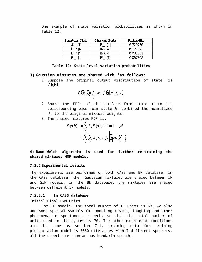
Table 20: Acoustic Classes for Manner of Articulation of Mandarin Initials. Classes distinguish between aspirated and unaspirated stops, aspirated and unaspirated fricatives, nasals, voiced and unvoiced fricatives, and laterals.

Table 21: Acoustic Classes for Place of Articulation of Mandarin Initials. Initials are distinguished as labial, alveolar, dental sibilants, retroflex, dorsal, and velar.

Table 22: Acoustic Classes for the Main Vowel of Mandarin Finals. Class names are derived in a straightforward manner from the IPA entry for the main vowel.

29

Table 23: Acoustic Classes for Vowel Content and Manner of Mandarin Finals. Classes distinguish monophones, diphthongs, and triphthongs that are open, rounded, stretched, or protruded.

Table 24: Acoustic Classes for Explicit Notation of Voicing for Mandarin Initials and Finals. Initials and finals are also distinguished in this attribute.

Table 25: Changes in Acoustic Features Yielding Non-Standard SAMPA-C Initials and Finals. Note that these account for only a small portion of the phonetic variability in the CASS corpus. Feature changes that yield a standard SAMPA-C form are not considered.

30

Table 26: CASS Initials Replaced by Nearest ’Standard’ Initial

As a result, the CASS SAMPA-C transcriptions contain annotated initials that are not in the pronunciation lexicon used to train the Broadcast News baseline system. Even within the CASS domain itself, these symbols are not found in the dominant pronunciation of any word. It is therefore not clear under what circumstances these variants should be preferred over pronunciations containing the standard phones. Given this uncertainty, it is difficult to train models for these symbols. Rather than develop a suitable training method for these unusual initials, we replaced them by their nearest ’standard’ initials, as shown in Table 26. We note that in the case of voicing changes, the substitution is not as exact as the transcription suggests, since the Mandarin initials are not usually voiced.

8.2.1 Annotation of Predictive Features

The use of annotation that indicates the present or absence of articulatory features suggests the possibility of directly measuring the features in the acoustic signal, by detecting voicing, nasalization and/or aspiration. For example, given the speech "bang fu", a voicing detector could be used to produce the automatically annotated form "b_v ang_v f_v u_v", indicating contextual voicing effects on the . In this way, the pronunciations derived by lexicon from a word transcription can be augmented by direct acoustic measurements of the speech. These measurements could be used to aid in the prediction, i.e. to provide additional side information to improve the choice of pronunciation by the ASR system. This side information could also be incorporated directly into the acoustic models, so that the choice of model changes depending on these direct acoustic measurements.

In our project this summer we studied only the use of voicing measurements. Voicing is also relatively easy to measure directly. Admittedly, much voicing information is already represented by the per-frame energy measurements in the cepstral acoustic features. Direct measurement of voicing may therefore not provide too much additional information. However, we take the view that if we can’t find at least small modeling improvements through direct measurement of voicing, it is unlikely that we will be successful with other acoustic features that are less easily measured.

8.2.1.1 Direct Measurement of VoicingUsing Entropic’s get_f0 pitch tracking program [19], a frame-by-frame voicing decision for the entire CASS corpus was computed (frames were 7.5msec with a 10msec step). The time segmentation in the GIF tier allows us to transform these per-frame decisions into segment-based probabilities of voicing, Pv, by counting the number of voiced frames and dividing by the total number of frames in the segment. This segment-based Pv can be turned into a hard decision for voicing by comparison to a threshold.

Initially, get_f0 was run with its default parameters. The performance of the automatic method was compared to linguist truth using a Detection Error Trade-off (DET) curve [20], which is shown in Figure 7(l). The individual performance for each speaker as well as the composite performance is shown. The point ’o’ on each curve is the detection performance when the threshold for voiced is chosen to be 0.5. The resulting segment-based voiced decision had variable speaker-dependent performance and a range of scores that did not generalize across

31

speakers for any single threshold value. This is likely due, at least in part, to the difficult acoustic conditions present in the CASS recordings.

It was observed, however, that in annotating the CASS corpus, the annotators mark that 60% of the data is voiced. We therefore identified the following procedure for normalizing the voicing detection: for each speaker, find a speaker-dependent threshold for the voice_bias parameter in get_f0 such that 60% of the segments had . For simplicity, only the threshold values 0.2, 0.4, 0.6, 0.8 are considered. The voice_bias parameter that gave the closet match to the 60% voiced criteria was chosen. No further tuning was performed. The score normalized DET is shown in Figure 7(r). The curves as well as the hard decision ’o’ points are more consistent across speakers than Figure 7(l), although there is still room for improvement.

The performance of this voicing detection scheme can be measured by comparison to voicing information inferred from the CASS transcriptions. We found an equal error point of 20% miss and 20% false alarm, which suggests the performance is quite consistent with that of the transcribers.

Figure 7: Voicing Detection Performance Without (l) and With (r) Speaker-Dependent Voice_bias Parameters.

8.2.2 Introducing Variability into the CASS Transcriptions

The SAMPA-C tier of the CASS corpus is a very accurate transcription of the acoustic data according to linguistic conventions developed at the Chinese Academy of Social Sciences. To non-expert listeners, however, these transcriptions tended to be very similar to dictionary-derived transcriptions. The consensus among the native Chinese speakers in our group is that the expert transcribers at CASS can find evidence for sounds by listening to the speech and studying spectrograms that casual listeners can not find.

This raises difficulties for our use of HMM acoustic models with these transcriptions. It is reasonable to question whether these acoustic models will be able to identify pronunciation changes that native (albeit inexpert) listeners are unable to detect. As expected, many of the initials and finals that casual listeners would prefer to delete are quite short according to the time segmentation in the SAMPA-C tier. This poses another difficulty for our acoustic models, which have a minimum duration imposed by the HMM topology. These models are not well suited for modeling acoustic segments of such short duration.

We chose to address these two problems by discarding the shortest initials and finals in the CASS transcriptions when building the pronunciation models. Our intent was to introduce

32

variability by removing the initials and finals from the transcription that we reasoned would be the most difficult to hear and to model.

A separate duration threshold is set for silence and non-silence segments: tokens of duration greater than or equal to the thresholds are kept. The silence and non-silence thresholds allow for some flexibility in selecting the speech to discard. Table 27 shows how the number of tokens is affected as the thresholds increase.

Table 27: Effect of Duration Thresholds. The percentage (and total number) of Silence and Nonsilence tokens that would be discarded by applying various duration thresholds.

Table 28: Introduction of Variability into the CASS Transcriptions. Diacritics are not considered in these measurements.

The experiments we report here are based on a 30 msec silence and a 20 msec nonsilence threshold. We also investigated a complex duration filter which attempts to join adjacent silence and non-silence tokens using the following rule: If the silence joins with a non-silence token to enable it to pass the non-silence threshold, then the silence is removed and the duration is updated for the non-silence token. The tokens would then be run through the simple duration filter.

As can be seen in Table 28 we are able to introduce significant variability into the CASS transcriptions in this manner. It may seem that discarding data in this way is fairly drastic. However, these transcriptions are used only to train the pronunciation models. They are not used to train acoustic models. In fact, despite this aggressive intervention the canonical pronunciations remain the dominant variant. However, in the acoustic alignment steps that use these models, the acoustic models will be allowed to chose alternative forms, if it leads to a more likely alignment than that of the canonical pronunciation.

8.3 PRONUNCIATION MODEL ESTIMATIONDuring the summer workshop we restricted ourselves to fairly straightforward pronunciation modeling experiments. Our goal was to augment and improve the baseline dictionary with pronunciation alternatives inferred from the CASS transcriptions. These new pronunciations are word_internal in that pronunciation effects do not span word boundaries. This is clearly less than ideal, however we are confident that if we can obtain benefit using relatively simple word-internal pronunciation models, we will find value in more ambitious models after the workshop.

33

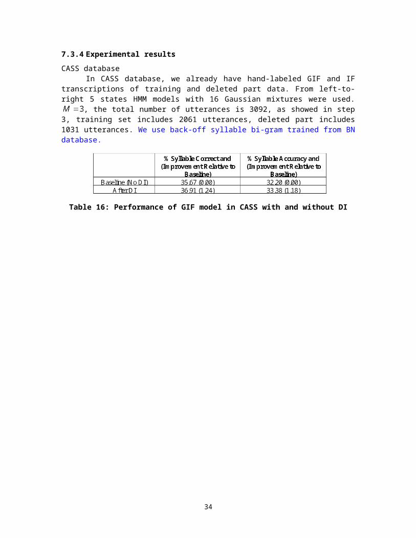
Table 29: Most Frequent Pronunciation Changes Observed in Aligning Mandarin Broadcast News Base-forms with Their Most Likely Surface Form as Found under the CASS Decision Tree Pronunciation Model. The symbol “-” indicates deletion.

8.3.1 CASS / Broadcast News Pronunciation Model Training Procedure

1. CASS Initial/Final Transcriptions: We began with alignments from the modified CASS corpus from which the short initials and finals were discarded as described in Table 27. An example of the aligned transcription is given here. As discussed previously, the goal is to use the direct voicing measurements to help predict surface forms. Therefore, only the base pronunciations are tagged with voicing information.

Utterance f0_0003:Surface Form: sil - uan d a i . . .Alignment Cost: 0 9 0 0 0 0 . . .Base Form: sil ch_u uan_v d_v a_v i_v . . .

The training set consisted of 3093 utterances, after discarding some utterances with transcription difficulties. The baseform initial/final transcriptions were derived from the Pinyin tier in the CASS transcriptions, and the surface forms were taken from CASS SAMPA-C tier. The initial and final entries have been tagged by the voicing detector, using the time marks in the CASS SAMPA-C tier, as described in Section 3.1.1. The baseform and surfaceform sequences were aligned, and the most frequent pronunciation changes are listed in Table 29.

2. CASS Decision Tree Pronunciation Models: The transcriptions described above form the training set that will be used to construct the initial decision tree pronunciation models to predict variations in the CASS data. The sequence of aligned initials and finals are transformed into a sequence of feature vectors. Each individual vector describes membership of its corresponding initial or final in broad acoustic classes, as described in Table 17-24. A separate decision tree is trained for each initial and final in the lexicon. The trees are grown under a minimum entropy criterion that measures the purity of the distribution at the leaf nodes; cross-validation is also performed over 10 subsets of the training corpus to refine the tree sizes and leaf distributions. This is described in [4]. Changes in each initial or final can

34

be predicted by asking questions about the preceding 3 and following 3 symbols. Questions about neighboring surface forms were not used.

Some basic analysis can be performed using these trees before they are applied to the Broadcast News corpus. The most frequent questions asked are given in Table 30 for trees trained both with and without voicing information; the former trees were constructed for this comparison, and were not otherwise used.

The quality of the trees can be evaluated by estimating the likelihood they assign to human annotated transcription on a held-out set of data. We used for this purpose the transcriptions of the 15-minute interlabeller agreement set, taking as truth the transcriptions provided by transcriber CXX. The log-likelihood of this held-out data is provided in Table 31. It can be seen that direct voicing information improves the overall likelihood of the human annotation, albeit only slightly.

3. Mandarin Broadcast News Pronunciation Lattices: The next step in the training procedure was to apply the CASS decision tree pronunciation models to acoustic training set transcriptions in the Mandarin Broadcast News corpus. This produced for each utterance a trellis (aka lattice) of pronunciation alternatives. The decision trees require voicing information, which is obtained using the voicing detector in the same manner as was done for the CASS data; time boundary information about the initials and finals in the baseform Broadcast News transcription was obtained via forced alignment. These trellises contain pronunciation alternatives for utterances in the Broadcast News training set based on pronunciation alternatives learned from the CASS transcriptions.

Table 30: Most Frequent Questions Used in the Construction of the CASS Decision Trees. The left-side data did not have access to voicing information. Positive numbers indicate right context, and negative numbers left context.

Table 31: Log-likelihood of Held-Out Interlabeller Agreement Corpus Evaluated using CASS Decision Tree Pronunciation Models Showing the Influence of Voicing in Predicting Pronunciation. The unigram model was found directly from the baseform/surfaceform alignments. The least likely 5% of the data were discarded (after [7]); unigram distributions were used for the rarely encountered insertions.

35

Table 32: Most Frequent Pronunciation Changes Observed in Aligning Mandarin Broadcast News Base-forms with Their Most Likely Surface Form as Found under the CASS Decision Tree Pronunciation Model. The symbol “-” indicates deletion.

4. Most Likely Pronunciation Alternatives under the CASS Decision Tree Pronunciation Models: Forced alignments via a Viterbi alignment procedure were performed using a set of baseline acoustic models that were trained using the baseform acoustic transcriptions (see Section 5). The forced alignment chose the most likely pronunciation alternative from the trellis of pronunciations generated by the CASS decision trees. The alignment was performed using two-component Gaussian mixture monophone HMMs to avoid using more complex models that might have been ’overly exposed’ to the baseform transcriptions in training.

These most likely alternatives are then aligned with the baseform pronunciations derived from the word transcriptions, shown in Table 32. In comparing these alignments with the alignments found within the CASS domain, we note an increased number of substitutions.

5. Most Likely Word Pronunciations under the CASS Decision Tree Pronunciation Models: The forced alignments yield alternative pronunciations for each entire utterance. In these initial experiments we wish to have only the pronunciation alternatives for individual words. We found these by first: 1) aligning the most likely pronunciation with the dictionary pronunciation to align the surface form phonetic with the words in the transcription; and then 2) tabulating the frequency with which alternative pronunciations of each word were observed. The result of this step is a Reweighted and Augmented CASS Dictionary tuned to the baseline Broadcast News acoustic Models.

6. Broadcast News Decision Tree Pronunciation Models: The alignments between the surface form initial/final sequence and the baseform initial/final sequence found by Viterbi can be used in training an entirely new set of decision tree pronunciation models. The surface initial/final sequences are the most likely pronunciation alternatives found under the CASS decision tree pronunciation models, as described above. As discussed earlier, this is a ’bootstrapping’ procedure. This second set of trees is not trained with surface form

36

transcriptions provided by human experts. They are however trained with approximately 10 hours of in-domain data, compared to the 2 hours of data available for training in the CASS transcriptions.

As shown in Table 33, questions about manner and place still dominate, as was found in the CASS decision trees. We cannot readily evaluate the predictive power of these trees we do not have available labeled data for the Broadcast News domain.

Table 33: Most Frequent Questions Used in the Construction of the Broadcast News Decision Trees. Positive numbers indicate right context, and negative numbers left context.

7. Most Likely Pronunciation Alternatives under Broadcast News Decision Tree Pronunciation Models: The decision tree pronunciation models obtained in the previous step can be applied to the Broadcast News acoustic training transcriptions. This produces for each utterance a trellis of pronunciation alternatives under the newly trained Broadcast News pronunciation models; these alternatives are a refinement of the first set of alternatives that were chosen from CASS pronunciation models. The most likely alternatives are chosen from these trellises by Viterbi alignment. The HMMs used for this operation are the same as those used in the previous alignment.

8. State-Level Surface Form to Base Form Alignments: An alternative Viterbi alignment can be per-formed to obtain an alignment at the state level between the surface form pronunciations and the baseform pronunciations. Unlike the previous alignment steps, this alignment uses a fully trained triphone HMM system. The Viterbi path is aligned against the baseform path at the state level. From this it can be determined which states are ’confusable’ under the pronunciation model. The most confusable states can be considered as candidates in soft-state clustering schemes. The simplest scheme is to 1) for each state in the HMM system, find the most confusable state in the surface form paths; 2) a copy of each Gaussian from this state is added to the Baseform mixture distribution; 3) several Baum Welch iterations are performed to update the means and mixture weights in the entire system.

This is the first HMM re-training step in the modeling procedure; all preceding steps are concerned with finding alternate pronunciations and refining the estimates of their frequencies.

9. Most Likely Word Pronunciations under the Broadcast News Decision Tree Pronunciation Models: A second Reweighted and Augmented Broadcast News Dictionary can be found in a manner identical to the first, except that the surface form pronunciations are chosen from trellises generated by the Broadcast News decision tree pronunciation models. A

37

new dictionary is then constructed to include the most frequent word pronunciation alternatives. While it might be hoped that this dictionary would be an improvement over the previous dictionary, that dictionary was also selected under the same set of HMMs. This dictionary is likely to be a refined version of the first reweighted dictionary.

As a summary, these training steps generate two Reweighted and Augmented Dictionaries. Both incorporate pronunciation alternatives chosen by Broadcast News acoustic models. They differ in that the pronunciations in the first dictionary are selected from alternatives presented by CASS decision tree pronunciation models, while the second dictionary is selected from alternatives from a Broadcast News pronunciation model; however, the pronunciations in both dictionaries are selected using the baseline Broadcast News HMMs. The relative frequencies used in each dictionary can be reestimated through forced alignment over the training data. The training procedure also generates a Soft-reclustering of the HMM triphone states based on confusability found under the pronunciation model.

8.4 MANDARIN BROADCAST NEWS LARGE VOCABULARY SPEECH RECOGNITION EXPERIMENTS

The baseline Mandarin ASR system was trained using a dictionary containing Pinyin pronunciations of words and individual characters provided by Thomas Zheng. This dictionary contains tone information in the pronunciations, however it was ignored; the baseline system was toneless. The dictionary contained 50,614 entries.

Table 34: Mandarin Broadcast News Corpus Broadcasts Used in Acoustic Training

The acoustic training set consisted of 10,483 utterances selected from the first two CDs in the LDC Mandarin 1997 Broadcast News distribution (see Table 34). Liu Yi selected these after he listened to them to verify that they did indeed contain standard Mandarin and not Mandarin from other dialects.

The word/character dictionary was used to segment the acoustic training set transcriptions to ensure that pronunciations were available for the entire training transcription. This also attempts to tune the pronunciations used during acoustic training to the dictionary that will be used during decoding. The word segmentations provided with the LDC corpus were not used. Baseline word, syllable (toneless pinyin), and initial/final transcriptions were derived for the training set using this segmentation and the supplied dictionary. The utterance segmentations provided by LDC were kept, however. The broadcasts were segmented into individual waveform files, and parameterized into Mel-frequency cepstral coefficients, along with first and second difference coefficients. The segmented utterances came to about 10 hours of data in total.

Context dependent initial/final models were trained using standard Baum Welch training and acoustic clustering procedures [11]. The HMM topology was left-to-right, without skips; models used for initials had three states, while models used for finals had four states. A global mean and variance were computed over the entire training corpus and used to initialize single-mixture Gaussians for all model states. The usual HTK flat-start procedure was used to build 12-mixture Gaussian, triphone state clustered HMMs with 2086 states. The acoustic equivalence classes listed in Table 35 and Table 36 were used in context-dependent HMM state clustering [11].

38

Class Name MembersInitial b p m f d t n l g k h j q x z c s zh ch sh rI_Obstruent b p f d t g k j q z c zh ch s sh x h rI_Sonorant m n lI_Affricate z zh j c ch qI_Stop b d g p t kI_UnAspStopAff b d g z zh jI_AspStopAff p t k c ch q kI_UnAspStop b d gI_AspStop p t kI_UnAspAff z zh jI_AspAff c ch qI_Nasal m nI_Fric f s sh r x hI_Labial b p f mI_Bilabial b p mI_Dentalveolar d t z c n s lI_Alveolar d t n lI_DentalSib z c sI_Retroflex zh ch sh rI_Dorsal x q jI_Velar h k g

Table 35: Candidate Acoustic Equivalence Classes for Mandarin Initials Used for Context-Dependent HMM State Clustering

39

Table 36: Candidate Acoustic Equivalence Classes for Mandarin Finals Used for Context-Dependent HMM State Clustering

40

8.4.1 Broadcast News Language Model

The text corpora listed in Table 37 were used to train word-level Broadcast News language model. The text was resegmented from its original distribution so that it agreed with the pronunciation lexicon, and the resulting number of in-vocabulary and out-of-vocabulary tokens are listed in Table 37. The SRI language modeling tools [21] were used to build a bigram language model. The resulting bigram contained 50,624 1-grams and 7,992,589 2-grams.

8.4.2 Broadcast News Baseline Test Set

Clean, unaccented utterances (F0 condition) from the 1997 and 1998 HUB-4NE test sets [22, 23]were selected as the evaluation test set. The resulting set contained 1263 utterances, with about 12,000 words. There were slightly more females than males, owing to anchor speech. The words in test set reference transcriptions were segmented into characters so that character error rate (CER) can be measured to assess recognizer performance. A very small number of utterances with OOV characters were excluded from the test set. The baseline results were obtained using the ATT Finite State Decoder [7] modified to HTK acoustic models. The Character Error Rate was 28.7%. For ease of experimentation, HTK lattices containing the bigram language model scores were derived from the ATT FSMs. Rescoring these lattices using the HTK HVite Viterbi decoder gives an identical CER baseline.

8.4.3 Performance of Mandarin Broadcast News Pronunciation Models

The pronunciation model to be evaluated is the Reweighted and Augmented CASS Dictionary described in Section 4.1. This dictionary consists of pronunciation alternatives for words, along with the number of observations of each alternative found in the 10 hour Broadcast News training corpus. Two parameters control the amount of pronunciation variability introduced: a Minimum Count parameter discards variants that occur with less than a fixed number of occurrences; and a Minimum Relative Frequency threshold discards relatively infrequent alternates, regardless of how frequently or infrequently they are observed. The performance of this dictionary with respect to these thresholds is given in Table 38. The second dictionary, estimated by finding the most frequent word pronunciations under the pronunciations produced by the Broadcast News decision tree pronunciation model, was also evaluated. However, it gave nearly identical results as the CASS-derived dictionary (Table 38).

The second set of pronunciation models evaluated were HMMs whose mixture weights and means were reestimated after Soft-reclustering of the HMM triphone states. Results are reported in Table 39. A significant 0.9% improvement in CER is found using the baseline dictionary. Furthermore, use of the reweighted and augmented dictionaries yields modest but clearly additive gains when used with these models for a full 1.2% CER reduction.

The best performance under these models was obtained with a Reweighted/Augmented CASS dictionary which was created using the baseline Broadcast News HMMs. This leads to a slight mismatch between the dictionary and the acoustic models used in decoding. It is possible that further improvements could be found by reweighting the pronunciation probabilities in either the Reweighted/Augmented CASS dictionary or the Reweighted/Augmented Broadcast News dictionary using these soft-clustered models.

41

Table 37: Text Source for Baseline Broadcast News Language Model. The word and out-of-vocabulary counts reflect resegmentation with respect to the pronunciation lexicon.

Table 38: Performance of Reweighted and Augmented CASS Dictionary on the Mandarin Broadcast News Test Set with Baseline Mandarin Acoustic Models. The total number of new pronunciations found in the dictionary is 6025. Only small changes in performance and the number of alternative pronunciations were noted with changes in thresholds. Pronunciation probabilities are scaled so that the maximum probability for each word is 1.0.

Table 39: Performance of Soft-Reclustering of HMM Triphone States. Decoding is performed first with the baseline dictionary and subsequently using the reweighted/augmented dictionary marked by * in Table 38.

42

9 ConclusionFrom our work over the summer, we can draw the following conclusions:

GIF better than IF on CASS even when data is sparse. Extending the canonical phoneme set gives us the ability to cover the sound changes in Mandarin and improves recognition accuracy.

The GIF lexicon needs to be augmented with probabilities. This is consistent with previous findings on probabilistic pronunciation lexicons.

Words are good (context is important). Intra-syllabic as well as inter-syllabic variations are important for modeling pronunciation in Mandarin spontaneous speech. Methods to find lexicon weights (CD equivalent class weighting helpful when data is sparse ) showing that context is important. Syllable ngrams derived from word information are useful across domain.

There are more sound changes than phone changes in CASS Mandarin (standard casual speech). The question remains whether these are transcription artifacts or due to standard Mandarin pronunciations without regional accents.

Sound changes are not lexical allophonic changes but due to casual speech in Mandarin spontaneous speech.

State level Gaussian sharing between IF with pronunciation probabilities can enrich phoneme models and is successful in improving recognition accuracy.

We also found that there is a high correlation between automatic voicing prediction and linguistic transcription

Direct acoustic feature that can be used without a pronunciation dictionary , framework established for incorporating direct measures into PM

Methods that work on conversational English also work on CASS with suitable modifications

Word pronunciations must be inferred directly rather than from syllable pronunciation changes

43

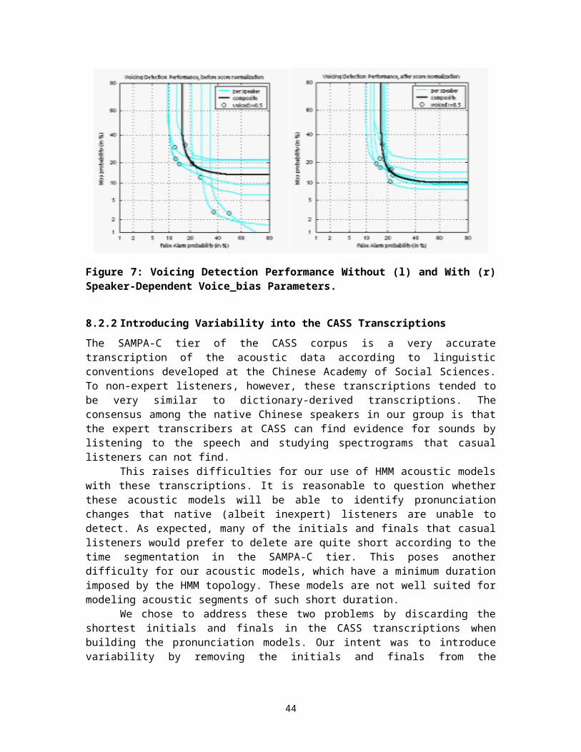
10 References[1] A. Li, F. Zheng, W. Byrne, P. Fung, T. Kamm, Y. Liu, Z. Song, U. Ruhi, V.

Venkataramani, and X. Chen, “CASS: A Phonetically Transcribed Corpus of Mandarin Spontaneous Speech,” presented at International Conference on Spoken Language Processing (ICSLP), Beijing, China, 2000.

[2] M. Riley, W. Byrne, M. Finke, S. Khudanpur, A. Ljolje, J. McDonough, H. Nock, M. Saraclar, C. Wooters, and G. Zavaliagkos, “Stochastic pronunciation modelling from hand-labelled phonetic corpora,” Speech Communication, vol. 29, pp. 209-224, 1999.

[3] M. Saraclar, H. Nock, and S. Khudanpur, “Pronunciation modeling by sharing Gaussian densities across phonetic models,” Computer Speech and Language, vol. 14, pp. 137-160, 2000.

[4] W. Byrne, M. Finke, S. Khudanpur, J. McDonough, H. Nock, M. Riley, M. Saraclar, C. Wooters, and G. Zavaliagkos, “A Status Report from WS97,” presented at IEEE Workshop on Automatic Speech Recognition and Understanding, Santa Barbara, CA, USA, 1997.

[5] Y. Liu and P. Fung, “Rule-based Word Pronunciation Network Generation for Mandarin Speech Recognition,” presented at International Symposium on Chinese Spoken Language Processing (ISCSLP), Beijing, China, 2000.

[6] Y. Liu and P. Fung, “Modeling Pronunciation Variations in Spontaneous Mandarin Speech,” presented at International Conference on Spoken Language Processing (ICSLP), Beijing, China, 2000.

[7] M. D. Riley and A. Ljolje, “Automatic Generation of Detailed Pronunciation Lexicons,” in Automatic Speech and Speaker Recognition: Advanced Topics, C.-H. Lee, F. K. Soong, and K. K. Paliwal, Eds. Norwell, MA: Kluwer Academic Publishers, 1995, pp. 285-301.

[8] X. Chen, A. Li, G. Sun, W. Hua, and Z. Yin, “An Application of SAMPA-C for Standard Chinese,” presented at International Conference on Spoken Language Processing (ICSLP), Beijing, China, 2000.

[9] A. Li, X. Chen, G. Sun, W. Hua, Z. Yin, and Y. Zu, “The Phonetic Labeling on Read and Spontaneous Discourse Corpora,” presented at International Conference on Spoken Language Processing (ICSLP), Beijing, China, 2000.

[10] M. Liu, B. Xu, T. Huang, Y. Deng, and C. Li, “Mandarin Accent Adaptation based on Context-Independent/Context-Dependent Pronunciation Modeling,” presented at International Conference on Acoustics, Speech and Signal Processing (ICASSP), Istanbul, Turkey, 2000.

[11] S. Young, D. Kershaw, J. Odell, D. Ollasen, V. Valtchev, and P. Woodland, The HTK Book: Version 2.2: Entropic Ltd., 1999.

[12] AT&T FSM Toolkit, http://www.research.att.com/sw/tools/fsm/

44

[13] F. Jelinek, Statistical Methods for Speech Recognition. Cambridge, MA: MIT Press, 1997.

[14] X. Huang, M.-Y. Hwang, L. Jiang, and M. Mahajan, “Deleted Interpolation and Density Sharing for Continuous Hidden Markov Models,” presented at International Conference on Acoustics, Speech and Signal Processing (ICASSP), Atlanta, Georgia, 1996.

[15] N. S. Kim and C. K. Un, “Statistically Reliable Deleted Interpolation,” IEEE Transactions on Speech and Audio Processing, vol. 5, pp. 292-5, 1997.

[16] TIMIT - Acoustic-Phonetic Continuous Speech Corpus, http://www.ldc.upenn.edu/

[17] S. Greenburg, “Speaking in Shorthand - A Syllable Centric Perspective for Understanding Pronunciation Variation,” presented at ESCA Workshop on Modeling Pronunciation Variation for Automatic Speech Recognition, Kekrade, Netherlands, 1998.

[18] M. Saraclar. “Pronunciation Modeling for Conversational Speech Recognition,” Ph.D. Thesis, Johns Hopkins University, Baltimore, MD, 2000.

[19] D. Talkin, “A Robust Algorithm for Pitch Tracking (RAPT),” in Speech Coding and Synthesis, W. B. Kleijn and K. K. Paliwal, Eds. New York: Elsevier, 1995.

[20] A. Martin, G. Doddington, T. Kamm, M. Ordowski, and M. Przybocki, “The DET Curve in Assessment of Detection Task Performance,” presented at 5th European Conference on Speech Communication and Technology (EUROSPEECH), Rhodes, Greece, 1997.

[21] SRILM - The SRI Language Modeling Toolkit, http://www.speech.sri.com/projects/srilm/

[22] 1997 Hub-4NE Mandarin NIST-evaluation, http://www.itl.nist.gov/iaui/894.01/tests/ctr/h5e_97/h5e_97.htm

[23] 1998 Hub-4NE Mandarin NIST-evaluation, http://www.itl.nist.gov/iaui/894.01/tests/ctr/hub5e_98/hub5e_98.htm

45