Delay Estimation and Fast Iterative Scheduling …baid/papers/WiOptTalkBaidFinal.pdfDelay Estimation...
22
Delay Estimation and Fast Iterative Scheduling Policies for LTE Uplink Akash Baid WINLAB, Rutgers University Ritesh Madan Accelera Mobile Broadband Ashwin Sampath Qualcomm
Transcript of Delay Estimation and Fast Iterative Scheduling …baid/papers/WiOptTalkBaidFinal.pdfDelay Estimation...

Delay Estimation and Fast Iterative Scheduling Policies for LTE Uplink
Akash Baid WINLAB, Rutgers University
Ritesh Madan Accelera Mobile Broadband
Ashwin Sampath Qualcomm
LTE Resource Allocation Problem →Motivation
○ System
Model
○ Problem
Formulation
○ Optimal
Solution
○ Simulation
Results
○ Conclusion
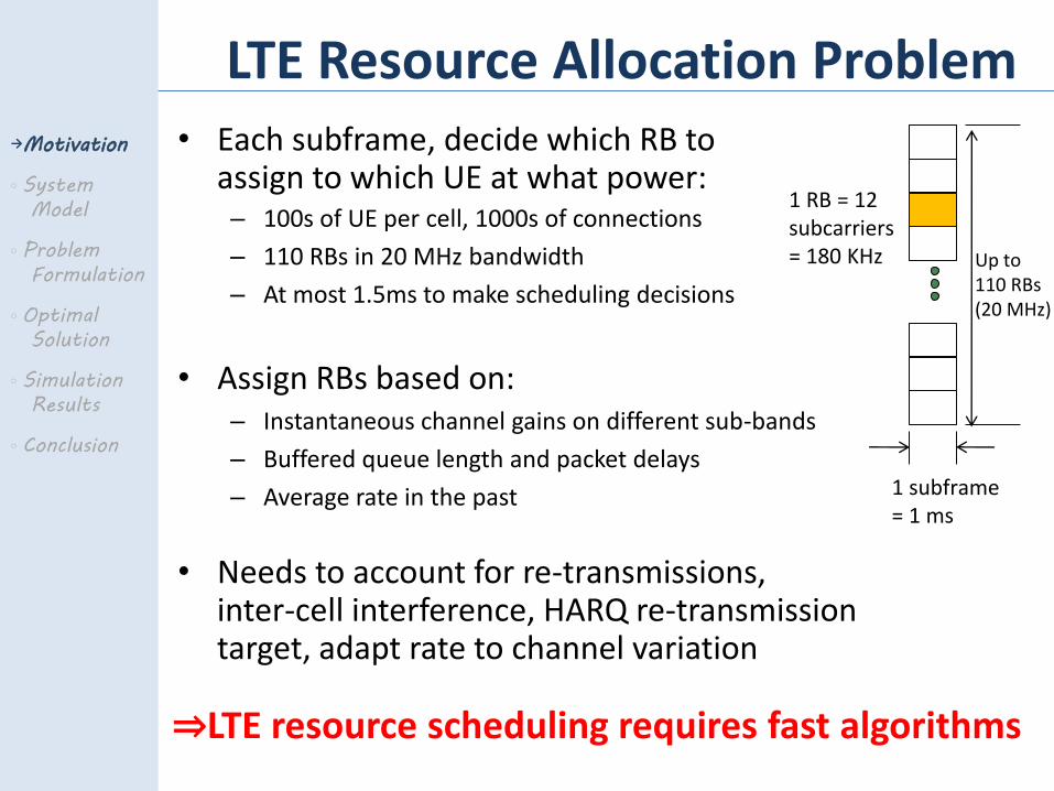
• Each subframe, decide which RB to assign to which UE at what power:
– 100s of UE per cell, 1000s of connections
– 110 RBs in 20 MHz bandwidth
– At most 1.5ms to make scheduling decisions
• Assign RBs based on: – Instantaneous channel gains on different sub-bands
– Buffered queue length and packet delays
– Average rate in the past
• Needs to account for re-transmissions, inter-cell interference, HARQ re-transmission target, adapt rate to channel variation
1 RB = 12 subcarriers = 180 KHz
1 subframe = 1 ms
Up to 110 RBs (20 MHz)
⇒LTE resource scheduling requires fast algorithms

Key Approaches in Scheduling Theory
→Motivation
○ System
Model
○ Problem
Formulation
○ Optimal
Solution
○ Simulation
Results
○ Conclusion
Max weight Schedulers:
Given instantaneous spectral efficiency 𝑠𝑖(𝑡), at each time step 𝑡, select the user with maximum 𝐾𝑖 𝑡 ∗ 𝑠𝑖(𝑡) and assign all resources to that user
- 𝐾𝑖 𝑡 could be function of:
- rate for elastic flows
- delay or queue length for delay-sensitive flows
- [Stoylar’04, Whiting’04]: this maximizes the sum-utility
of long term average rates
- [Tassiulas’93]: maximizing queue length times rate
leads to stable queues

→Motivation
○ System
Model
○ Problem
Formulation
○ Optimal
Solution
○ Simulation
Results
○ Conclusion
- In large bandwidth systems, iterative algorithms allow more users to be multiplexed, lowers delay [Bodas’10, Lin’11]
- But past results based on restrictive models: No power and interference constraints; on-off rate model
Key Approaches in Scheduling Theory
Iterative Scheduling: Make assignments 1 RB at a time; assign user with maximum recompute assign the next RB in the same way to (potentially) different user

Our Contributions
Generalize delay based iterative schedulers to the LTE uplink system model via a novel objective function
Obtain low complexity iterative algorithms
Sub-gradient analysis for frequency flat fading
Specialized interior point method for frequency selective fading
Design a novel mechanism for inferring packet delays approximately from buffer status reports
Demonstrate performance via detailed LTE simulations
→Motivation
○ System
Model
○ Problem
Formulation
○ Optimal
Solution
○ Simulation
Results
○ Conclusion

LTE Uplink System Model
• Single Carrier FDMA with 180 kHz x 1 ms RB
• We consider M sub-bands of equal bandwidth B, with B < coherence bandwidth of each user
• Constraints : – Fractional power control: limits inter-cell interference
– Peak power constraint: from regulatory requirements
– Total bandwidth: based on available bandwidth
– Achievable rate:
○ Motivation
→System
Model
○ Problem
Formulation
○ Optimal
Solution
○ Simulation
Results
○ Conclusion

Estimating Delay from BSR ○ Motivation
→System
Model
○ Problem
Formulation
○ Optimal
Solution
○ Simulation
Results
○ Conclusion
• UEs send periodic Buffer Status Report (BSR) with info about no. of total bytes in buffer
• We use the BSR reports along with knowledge of number of bytes scheduled in each subframe to estimate the packet delays:
• Main complexity is due to re-transmissions which can lead to BSR report arriving out of order
0 1 2 3 4 5 6 7 9 8
0 1 2 3 4 5 6 7 9 8
BSR = 100 75 Bytes
eNB
UE
BSR = 50 implies 25 bytes arrived

Reward Functions ○ Motivation
○ System
Model
→Problem
Formulation
○ Optimal
Solution
○ Simulation
Results
○ Conclusion
Scheduler aims to maximize , defined as:
• Best Effort:
–
– , strictly concave increasing function
Reward Functions ○ Motivation
○ System
Model
→Problem
Formulation
○ Optimal
Solution
○ Simulation
Results
○ Conclusion
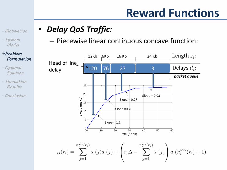
• Delay QoS Traffic:
– Piecewise linear continuous concave function:
0 10 20 30 40 50 600
5
10
15
20
25
rate (Kbps)
rew
ard
(m
sK
b)
Slope = 1.2
Slope =0.76
Slope = 0.27
Slope = 0.03
120 76 27 3
12Kb 6Kb 16 Kb 24 Kb Length 𝑠𝑖:
Delays 𝑑𝑖:
packet queue
Head of line delay

Frequency Flat Fading
• Given a total of B RBs, we want to solve:
– Convex problem but non-differentiable objective
• Solution through Lagrange dual problem
– There exists a s.t. the following are equalized :
– For B.E. users: marginal utility x incremental rate
– For Delay QoS users: HoL delay x incremental rate
– 𝑂 𝑁 log 𝐿 for 𝑁 users and 𝐿 points of discontinuity
○ Motivation
○ System
Model
○ Problem
Formulation
→Optimal
Solution
○ Simulation
Results
○ Conclusion

Computation of optimal solution
• The optimal solution can be found through a bisection search on the sub-gradient; however: – Discontinuity due to max power could result in convergence to
unstable points
– Discontinuity due to design of delay utility function could result in non-convergence of bisection search
○ Motivation
○ System
Model
○ Problem
Formulation
→Optimal
Solution
○ Simulation
Results
○ Conclusion
Two user example:
Packet Delays
U1 450 330 …
U2 170 150
threshold
U1 5
U2 8

Simulation Framework & Topologies
• Detailed system simulator:
– PHY layer performance (channel, power, rate)
– MAC layer signaling
– 19 cell simulation with wrap around to compute IoT
– Single cell simulation to calculate resulting rate, delay
• Mix of two types of traffic:
– Live Video: On-Off Markov model, 300 kbps when On
– Streaming Video: packet inter-arrival time, packet length both drawn from truncated Pareto distr., adaptive rate streaming with mean rate at 80% of achievable rate at full buffer
○ Motivation
○ System
Model
○ Problem
Formulation
○ Optimal
Solution
→Simulation
Results
○ Conclusion

HoL Delay Estimation
• Delay estimation performance over a 1 second run for a particular UE in a 20 UE simulation.
• Main source of error is the difference in the time at which UE and BS updates its delay counters
○ Motivation
○ System
Model
○ Problem
Formulation
○ Optimal
Solution
→Simulation
Results
○ Conclusion

Delay performance
• Comparing three scheduling algorithms:
– Non-iterative maximum weight: a UE with the highest queue length times spectral efficiency for first RB is allocated bandwidth until the queue is drained or the UE becomes power limited before allocation to the next UE.
– Iterative Queue: minimizes sum-of-squares of queue lengths [8]
– Iterative Delay: maximizes the reward function we defined above
○ Motivation
○ System
Model
○ Problem
Formulation
○ Optimal
Solution
→Simulation
Results
○ Conclusion

Delay performance ○ Motivation
○ System
Model
○ Problem
Formulation
○ Optimal
Solution
→Simulation
Results
○ Conclusion
Median delays 95 percentile delays10
1
102
103
De
lay (
millise
co
nd
s)
Median delays 95 percentle delays10
1
102
103
104
De
lay (
millise
co
nd
s)
Non-Iterative Iterative Queue-based Iterative Delay-based
• Macro-cell simulation: 20 UEs with pathloss between 100 dB and 135 dB
Live Video Users Streaming Video Users
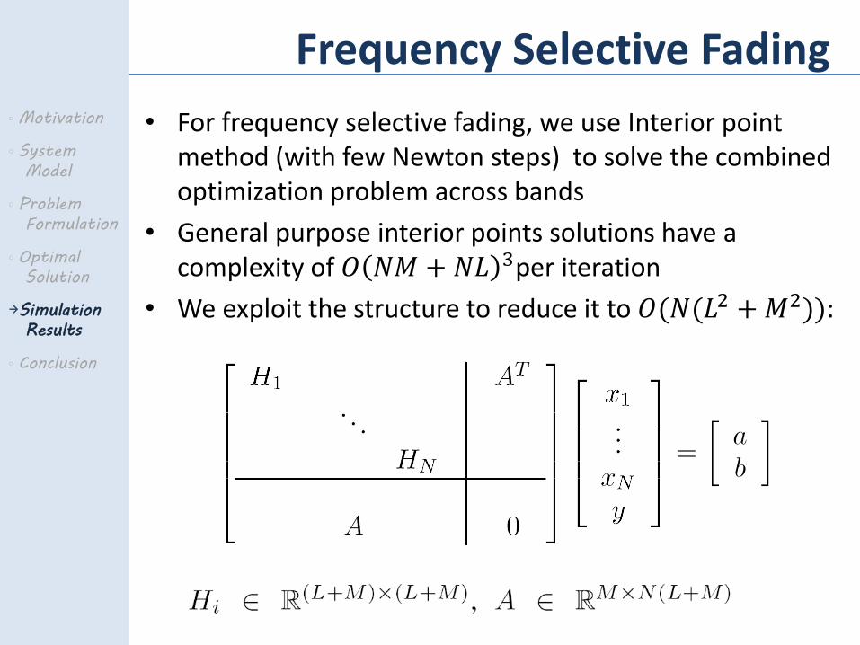
Frequency Selective Fading
• For frequency selective fading, we use Interior point method (with few Newton steps) to solve the combined optimization problem across bands
• General purpose interior points solutions have a complexity of 𝑂 𝑁𝑀 + 𝑁𝐿 3per iteration
• We exploit the structure to reduce it to 𝑂(𝑁(𝐿2 + 𝑀2)):
○ Motivation
○ System
Model
○ Problem
Formulation
○ Optimal
Solution
→Simulation
Results
○ Conclusion

Conclusions
• LTE resource allocation problems require low complexity algorithms
• A general iterative framework with different utility functions for different traffic types can be used to achieve respective goals
• Exploiting the structure of the problem can lead to design of fast scheduling algorithms: – per iteration for frequency flat fading
– per iteration for frequency selective
• Simulation shows the benefit of iterative HoL delay based scheduling over non-iterative and iterative queue-based scheduling
○ Motivation
○ System
Model
○ Problem
Formulation
○ Optimal
Solution
○ Simulation
Results
→ Conclusion

Thanks !
Questions ?

Extras
Estimating Delay from BSR ○ Motivation
→System
Model
○ Problem
Formulation
○ Optimal
Solution
○ Simulation
Results
○ Conclusion
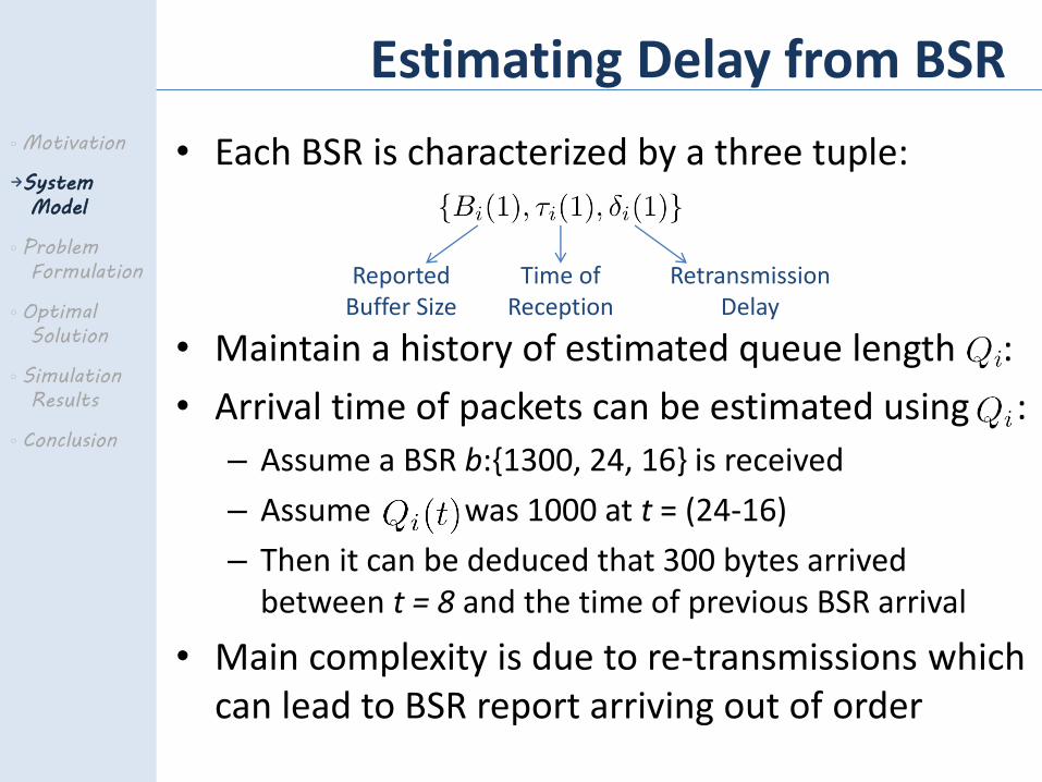
• Each BSR is characterized by a three tuple:
• Maintain a history of estimated queue length :
• Arrival time of packets can be estimated using :
– Assume a BSR b:{1300, 24, 16} is received
– Assume was 1000 at t = (24-16)
– Then it can be deduced that 300 bytes arrived between t = 8 and the time of previous BSR arrival
• Main complexity is due to re-transmissions which can lead to BSR report arriving out of order
Reported Buffer Size
Time of Reception
Retransmission Delay

Estimating Delay from BSR ○ Motivation
→System
Model
○ Problem
Formulation
○ Optimal
Solution
○ Simulation
Results
○ Conclusion
• Maintain a history of estimated queue length 𝑄𝑖(𝑡)
• 𝑄𝑖(𝑡) entries are updated according to:
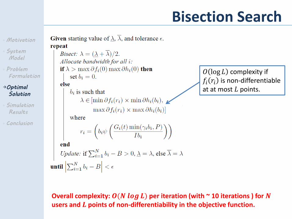
Bisection Search ○ Motivation
○ System
Model
○ Problem
Formulation
→Optimal
Solution
○ Simulation
Results
○ Conclusion
𝑂 log 𝐿 complexity if 𝑓𝑖 𝑟𝑖 is non-differentiable at at most 𝐿 points.
Overall complexity: 𝑶(𝑵 𝒍𝒐𝒈 𝑳) per iteration (with ~ 10 iterations ) for 𝑵 users and 𝑳 points of non-differentiability in the objective function.