Delaunay Triangulation Algorithm and Application to Terrain ...

Delaunay Triangulation Algorithm and Application to Terrain

Generation

Faniry Harijaona Razafindrazaka ([email protected])African Institute for Mathematical Sciences (AIMS)

Supervised by: Doctor J W Sanders

International Institute for Software Technology

United Nations University, Macao

22 May 2009

Submitted in partial fulfillment of a postgraduate diploma at AIMS

Abstract

We describe a randomized incremental algorithm for computing the Delaunay triangulation of a set ofpoints and a recent technique of applying it to terrain generation. The algorithm is optimal, using aDirected Acyclic Graph (DAG)-based location structure for the incremental insertion which achieves anexpected running time of O(n log n) and O(n) expected storage. The analysis of the expected storage issimplified, and the algorithm is implemented and tested. The implementation is done, in its integrality,with CGAL-Python which is fast and friendly, followed by numerical statistics on different distributions.The terrain generation technique is based on gaussian functions and the plotting is made with the OpenSource software Blender 3D which is probably its first combination with CGAL-Python. A high qualityrendering of three simple terrains is shown as a demonstration of the terrain generator.

Mamaritra tetika fanamboarana ny fanatelozoroan’ i Delaunay ao aminy velarana R2 amin’ny fomba

kisendrasendra isika ary ny fampiasana azy io aminy famoronana vohitra. Ilay tetika dia maty paika izaymampiasa grafy misy toro-lalana ary tsy misy fihodonana aminy fanatsofoana ireo teboka isan’isany,ny fandalinana ny hafainganany kosa dia natao faran’izay tsotra. Ny famolavolana dia natao, aminyakapobeny, tamin’ny CGAL-Python izay aingana sady mora ampiasaina, ny vokatra numerika dia nomenaihany koa. Ilay fanamboarana vohitra dia tsy voafetra izay afaka mamboatra tendrombohitra arak’izayilainy mpampiasa. Ilay vohitra dia natao kisary tamin’ilay fitaovana maimaimpona Blender 3D izay metyho voalohany aminy fampiasana azy io sy CGAL-Python miaraka. Hisy vohitra roa haseho aminy endrinyfarany izay kanto mba anehoana ny fahatsaran’ilay fanamboarana.

Declaration

I, the undersigned, hereby declare that the work contained in this essay is my original work, and thatany work done by others or by myself previously has been acknowledged and referenced accordingly.

Faniry Harijaona Razafindrazaka, 22 May 2009

i

Contents

Abstract i

1 Introduction 1

2 Voronoi diagram and Delaunay triangulation 2

2.1 The Voronoi diagram . . . . . . . . . . . . . . . . . . . . . . . . . . . . . . . . . . . . 2

2.1.1 Voronoi Cells . . . . . . . . . . . . . . . . . . . . . . . . . . . . . . . . . . . . 2

2.1.2 Example . . . . . . . . . . . . . . . . . . . . . . . . . . . . . . . . . . . . . . . 2

2.1.3 Half-Planes . . . . . . . . . . . . . . . . . . . . . . . . . . . . . . . . . . . . . 2

2.2 Dual of V (P) . . . . . . . . . . . . . . . . . . . . . . . . . . . . . . . . . . . . . . . . 3

2.2.1 Construction . . . . . . . . . . . . . . . . . . . . . . . . . . . . . . . . . . . . . 3

2.2.2 Duality Properties . . . . . . . . . . . . . . . . . . . . . . . . . . . . . . . . . . 3

2.3 The Delaunay triangulation . . . . . . . . . . . . . . . . . . . . . . . . . . . . . . . . . 4

3 The Algorithm 7

3.0.1 Basic Concepts . . . . . . . . . . . . . . . . . . . . . . . . . . . . . . . . . . . 7

3.0.2 Why Randomized Incremental Algorithm? . . . . . . . . . . . . . . . . . . . . . 7

4 Computation of the Delaunay Triangulation 9

4.1 Initialisation of the Three Dummy Points . . . . . . . . . . . . . . . . . . . . . . . . . . 9

4.2 The Delaunay Tree . . . . . . . . . . . . . . . . . . . . . . . . . . . . . . . . . . . . . 9

4.3 Legalization . . . . . . . . . . . . . . . . . . . . . . . . . . . . . . . . . . . . . . . . . 11

4.4 Efficient Incremental Algorithm . . . . . . . . . . . . . . . . . . . . . . . . . . . . . . . 11

4.5 Correctness and Efficiency . . . . . . . . . . . . . . . . . . . . . . . . . . . . . . . . . . 12

5 Applications 18

5.0.1 Vertices-and-Faces-Based Datastructure . . . . . . . . . . . . . . . . . . . . . . 18

5.0.2 Statistics . . . . . . . . . . . . . . . . . . . . . . . . . . . . . . . . . . . . . . . 18

5.1 Terrain Generation . . . . . . . . . . . . . . . . . . . . . . . . . . . . . . . . . . . . . . 20

5.1.1 What is a Terrain? . . . . . . . . . . . . . . . . . . . . . . . . . . . . . . . . . 20

5.1.2 The Modelling Technique . . . . . . . . . . . . . . . . . . . . . . . . . . . . . . 20

5.1.3 The Terrain Generator . . . . . . . . . . . . . . . . . . . . . . . . . . . . . . . 21

ii

5.1.4 Main Idea . . . . . . . . . . . . . . . . . . . . . . . . . . . . . . . . . . . . . . 21

5.1.5 The Process of Construction . . . . . . . . . . . . . . . . . . . . . . . . . . . . 21

5.1.6 Visualisation . . . . . . . . . . . . . . . . . . . . . . . . . . . . . . . . . . . . . 22

6 Notes and Comments 26

References 28

iii

1. Introduction

The Delaunay triangulation of a set of points is one of the classical problems in computational geometry.It was discovered in 1934 by the French mathematician Boris Nikolaevich Delone or Delaunay [2]. Manyalgorithms have since been proposed by computer scientists as well as mathematicians. In 1985, Guibasand Stolfi [10] proposed a Divide and Conquer algorithm which achieves the optimal bound of O(n log n).Later on, Steve Fortune [7] proposed a Sweepline algorithm for Voronoi diagrams which also achieves thisbound. Unfortunately, they are hard to implement, so that engineers instead use incremental insertionalgorithms because of their simplicity and the fact that they are not hard to implement. Guibas and Stolfi[10] proposed an incremental algorithm using a walking strategy to locate points which achieves O(n1/2)per point location, and it was improved by Mucke [6] to an O(n1/3) per point location. Although thesealgorithms provide good implementations, they are still sub-optimal algorithms. Thus we will presentan optimal randomized incremental algorithm which uses a DAG-based data structure for the pointlocation, using the analysis proposed in [9] and which solves the problem in O(n log n) expected timeand O(n) expected storage.

Nowadays, generating artificial terrains are indispensable. They are used in flight simulator, in makingtexture map to use as a background, in creating virtual worlds in game programming as well as in 3Danimated movies. They are many ways to generate them, a simple randomize-and-smooth technique[13] can be used, or a more complicated way is based on fractal methods [16], whereas fluid simulationcan also be used [16]. In this report, we present a recent technique based on gaussian functions andthe Delaunay triangulation. The statistics parameters of the gaussian enable us to control the qualityand the quantity of features in the heighten map.

The report follows the general approach of randomized incremental construction of the Delaunay trian-gulation, but differs in the following respects:

(i) the analysis of the expected storage is proved by backwards analysis;

(ii) the implementation is done with CGAL-python combined with Blender 3D which makes the drawingeasier and produces results of high quality;

(iii) a technique of generating terrain based on the Delaunay triangulation is developed.

The work is divided in two parts. The first part introduces the definition of Delaunay triangulation andthe theoretical analysis of the algorithm, while the second part is its application to terrain generation.The Delaunay triangulation is known to be the dual of the Voronoi diagram, as described in Chapter2. We then study some properties of a Delaunay triangle from the empty circle criterion to the localmax-min angle criterion. In Chapter 3, several algorithms are given and contrasted with the randomizedincremental method, especially the Divide and Conquer algorithm [10] and the Plane Sweep algorithm[7]. The location structure is explained in Chapter 4 with the DAG-based datastructure, followed bypseudo code of the full algorithm. The analysis of the algorithm is simplified as much as possible, usingbasic tools from probability and backwards analysis. Finally, in Chapter 5, statistics on the speed of thepoint location are given, and the application of the Delaunay triangulation to the perspective view oftopographic maps is explained. We then develop one method to generate terrain.

1

2. Voronoi diagram and Delaunay triangulation

In this section, we first introduce the notion of Voronoi cells and half-planes, and then give the dualityproperties of the Delaunay triangulation.

2.1 The Voronoi diagram

2.1.1 Voronoi Cells

Let P = p1, p2, p3, . . . , pn be a set of points in the Euclidian plane which are called the sites. A regionof the plane obtained by assigning every point to its nearest site pi is called the Voronoi cell V(pi), thatis,

V(pi) = x ∈ R2 : d(x, pi) ≤ d(x, pj), ∀i 6= j.

It can be interpreted as the set of all points which are closer to pi than the other sites. Some pointsdo not have an unique nearest site or nearest neighbor. The set of all points that have more than onenearest neighbor is called the Voronoi diagram V (P) for the set of sites.

2.1.2 Example

Consider three sites in the plane. Geometrically, the Voronoi diagram of these three sites is the per-pendicular bisectors of the three sides of the triangle formed by the three (non-collinear) points whichintersect at the circumcenter, the center of the unique circle that passes through the triangle’s vertices.Thus the Voronoi diagram for three points must appear as in Figure 2.1.

pi

pj

pk

Bik

Bij

Bkj

V (P)

pipj

pk

V (P)

Figure 2.1: Three sites: bisectors meet at the circumcenter

2.1.3 Half-Planes

Let H(pi, pj) be the closest half-plane bounded by Bij and containing pi (Figure 2.1). We can interpretH(pi, pj) as,

H(pi, pj) = x ∈ R2 | d(x, pi) < d(x, pj), for i 6= j,

2

Section 2.2. Dual of V (P) Page 3

Using this notation for the definition of the Voronoi diagram, we have that

V(pi) =⋂

j 6=i

H(pi, pj).

The intersection is taken over all j’s which are different from i. We will use this characterisation of theVoronoi diagram later on.

2.2 Dual of V (P)

Definition 2.2.1. The dual of a planar graph G is constructed as follows: each face in G is representedby a vertex, and for each edge e ∈ E(G), we draw an edge between the vertices that represent the faceswhich share the edge e.

Definition 2.2.2. A triangulation of a set of point P is defined to be a planar subdivision S such thatadding an edge connecting two points of P which is not in S will destruct its planarity.

2.2.1 Construction

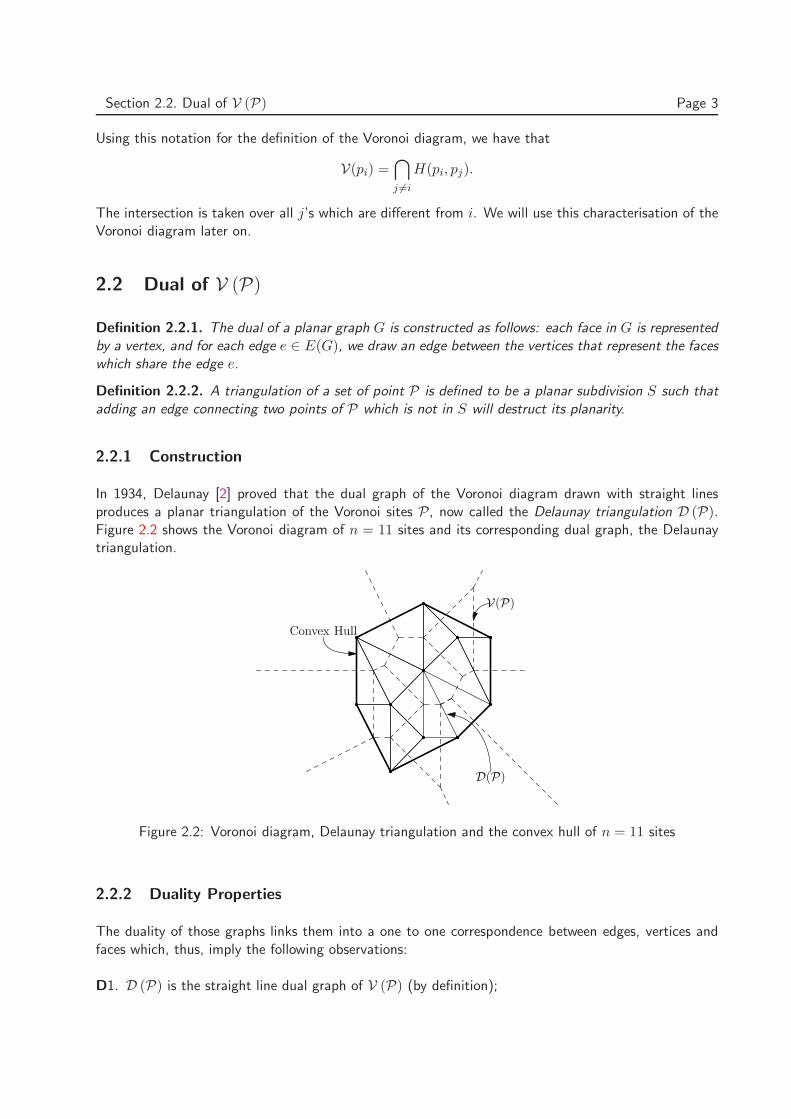
In 1934, Delaunay [2] proved that the dual graph of the Voronoi diagram drawn with straight linesproduces a planar triangulation of the Voronoi sites P, now called the Delaunay triangulation D (P).Figure 2.2 shows the Voronoi diagram of n = 11 sites and its corresponding dual graph, the Delaunaytriangulation.

Convex Hull

V(P)

D(P)

Figure 2.2: Voronoi diagram, Delaunay triangulation and the convex hull of n = 11 sites

2.2.2 Duality Properties

The duality of those graphs links them into a one to one correspondence between edges, vertices andfaces which, thus, imply the following observations:

D1. D (P) is the straight line dual graph of V (P) (by definition);

Section 2.3. The Delaunay triangulation Page 4

D2. D (P) is a triangulation if no four points of P are cocircular (see Remark 2.3.2);

D3. every triangle of D (P) corresponds to a vertex of V (P);

D4. each edge of D (P) corresponds to an edge of V (P);

D5. each node of D (P) corresponds to a region of V (P);

D6. The boundary of D (P) is the convex hull1 of the sites P (Figure 2.2);

D7. The interior of each triangle face of D (P) contains no site.

Remark 2.2.3. Properties D6 and D7 are the most interesting and can be verified in Figure 2.2.Property D7 has its equivalence in the property of Voronoi diagram saying that the circumcircle ofevery three sites contains no other sites [15].

2.3 The Delaunay triangulation

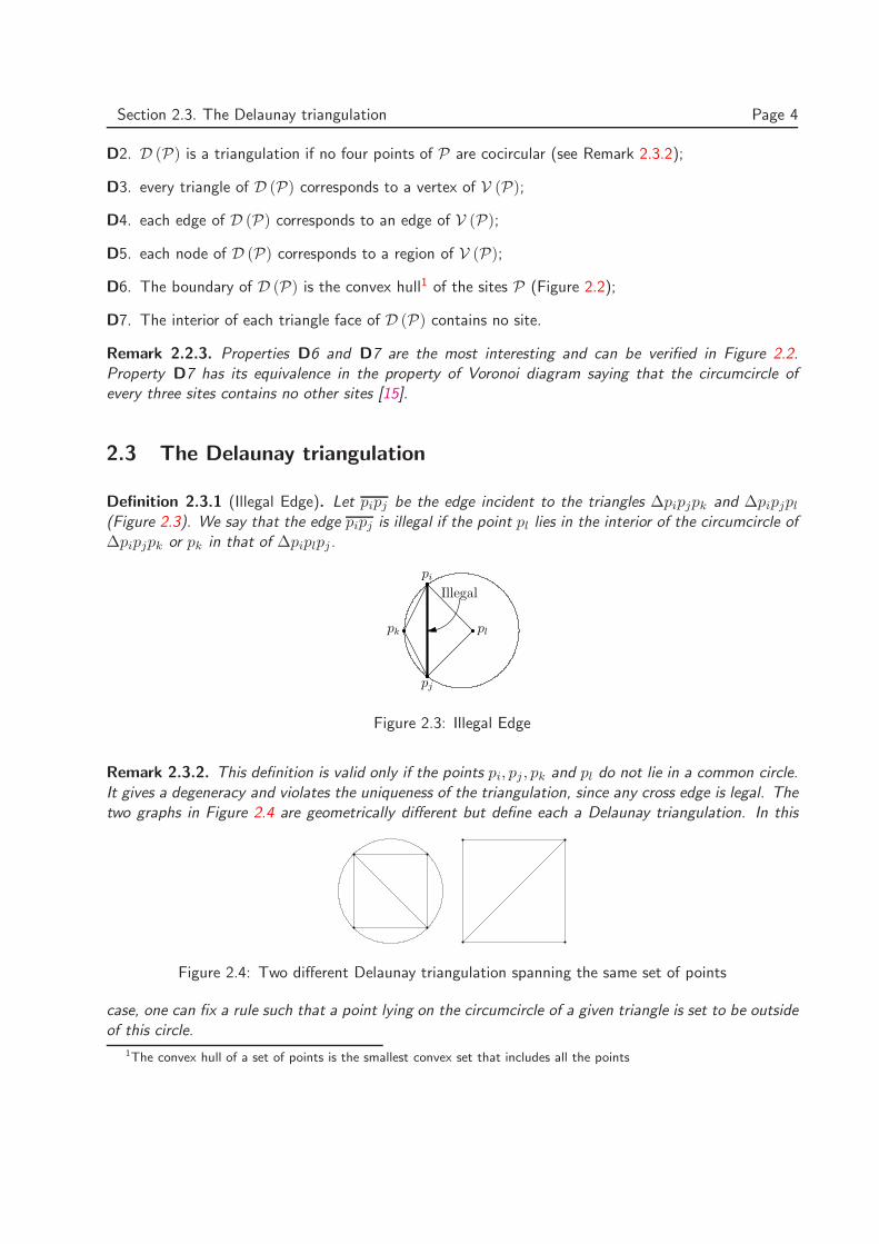
Definition 2.3.1 (Illegal Edge). Let pipj be the edge incident to the triangles ∆pipjpk and ∆pipjpl

(Figure 2.3). We say that the edge pipj is illegal if the point pl lies in the interior of the circumcircle of∆pipjpk or pk in that of ∆piplpj.

Illegal

pk

pj

pl

pi

Figure 2.3: Illegal Edge

Remark 2.3.2. This definition is valid only if the points pi, pj , pk and pl do not lie in a common circle.It gives a degeneracy and violates the uniqueness of the triangulation, since any cross edge is legal. Thetwo graphs in Figure 2.4 are geometrically different but define each a Delaunay triangulation. In this

Figure 2.4: Two different Delaunay triangulation spanning the same set of points

case, one can fix a rule such that a point lying on the circumcircle of a given triangle is set to be outsideof this circle.

1The convex hull of a set of points is the smallest convex set that includes all the points


Definition 2.3.3 (The empty circle criterion). Given a triangulation T of a set of points P, if thecircumcircle of a triangle in the triangulation is an empty circle, we say that the triangle satisfies theempty circle criterion.

This empty circle criterion is equivalent to the fact that every edge in the triangulation is legal. Thetriangle in Figure 2.3 do not satisfy the empty circle criterion.

Theorem 2.3.4 (The empty circle theorem). Let P be a set of points in the plane. A triangulation Tof P satisfies the empty circle criterion if and only if T is a Delaunay triangulation of P.

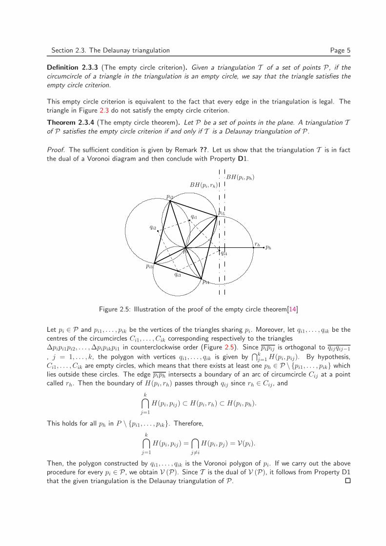
Proof. The sufficient condition is given by Remark ??. Let us show that the triangulation T is in factthe dual of a Voronoi diagram and then conclude with Property D1.

pi2

pi3

pi4

pi1

pi

qi1

qi2

qi3

qi4

ph

BH(pi, rh)

BH(pi, ph)

rh

Figure 2.5: Illustration of the proof of the empty circle theorem[14]

Let pi ∈ P and pi1, . . . , pik be the vertices of the triangles sharing pi. Moreover, let qi1, . . . , qik be thecentres of the circumcircles Ci1, . . . , Cik corresponding respectively to the triangles∆pipi1pi2, . . . ,∆pipikpi1 in counterclockwise order (Figure 2.5). Since pipij is orthogonal to qijqij−1

, j = 1, . . . , k, the polygon with vertices qi1, . . . , qik is given by⋂k

j=1 H(pi, pij). By hypothesis,Ci1, . . . , Cik are empty circles, which means that there exists at least one ph ∈ P \pi1, . . . , pik whichlies outside these circles. The edge piph intersects a boundary of an arc of circumcircle Cij at a pointcalled rh. Then the boundary of H(pi, rh) passes through qij since rh ∈ Cij, and

k⋂

j=1

H(pi, pij) ⊂ H(pi, rh) ⊂ H(pi, ph).

This holds for all ph in P \ pi1, . . . , pik. Therefore,

k⋂

j=1

H(pi, pij) =⋂

j 6=i

H(pi, pj) = V(pi).

Then, the polygon constructed by qi1, . . . , qik is the Voronoi polygon of pi. If we carry out the aboveprocedure for every pi ∈ P, we obtain V (P). Since T is the dual of V (P), it follows from Property D1that the given triangulation is the Delaunay triangulation of P.


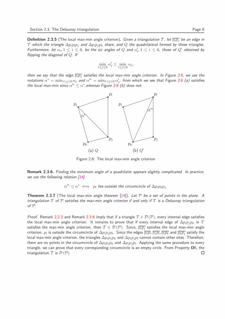
Definition 2.3.5 (The local max-min angle criterion). Given a triangulation T , let pipj be an edge inT which the triangle ∆piplpj and ∆pipjpk share, and Q the quadrilateral formed by these triangles.Furthermore, let αi, 1 ≤ i ≤ 6, be the six angles of Q and α′

i, 1 ≤ i ≤ 6, those of Q′ obtained byflipping the diagonal of Q. If

min1≤j≤6

α′j ≤ min

1≤j≤6αj ,

then we say that the edge pipj satisfies the local max-min angle criterion. In Figure 2.6, we use thenotations α∗ = min1≤j≤6 αj and α′∗ = min1≤j≤6 α′

j, from which we see that Figure 2.6 (a) satisfiesthe local max-min since α′∗ ≤ α∗,whereas Figure 2.6 (b) does not.

pi

α∗

pj

pk

pl

pi

α′∗

pj

pk

pl

(a) Q (b) Q′

Figure 2.6: The local max-min angle criterion

Remark 2.3.6. Finding the minimum angle of a quadrilater appears slightly complicated. In practice,we use the following relation [14].

α′∗ ≤ α∗ ⇐⇒ pl lies outside the circumcircle of ∆pipkpj.

Theorem 2.3.7 (The local max-min angle theorem [14]). Let P be a set of points in the plane. Atriangulation T of P satisfies the max-min angle criterion if and only if T is a Delaunay triangulationof P.

Proof. Remark 2.2.3 and Remark 2.3.6 imply that if a triangle T ∈ D (P), every internal edge satisfiesthe local max-min angle criterion. It remains to prove that if every internal edge of ∆pipjpk in Tsatisfies the max-min angle criterion, then T ∈ D (P). Since, pipj satisfies the local max-min anglecriterion, pl is outside the circumcircle of ∆pipjpk. Since the edges pipl, pjpl, pipk and pkpj satisfy thelocal max-min angle criterion, the triangles ∆pipjpk and ∆pipjpl cannot contain other sites. Therefore,there are no points in the circumcircle of ∆pipjpk and ∆pipjpl. Applying the same procedure to everytriangle, we can prove that every corresponding circumcircle is an empty circle. From Property D6, thetriangulation T is D (P).

3. The Algorithm

Having described the Delaunay triangulation, we introduce here an optimal algorithm which computesdirectly the Delaunay triangulation of a set of points in the plane. The algorithm is in the class ofrandomized incremental constructions and will be contrasted with other optimal algorithms.

3.0.1 Basic Concepts

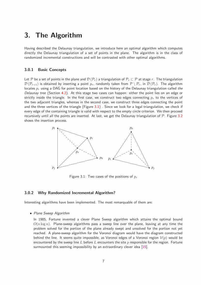
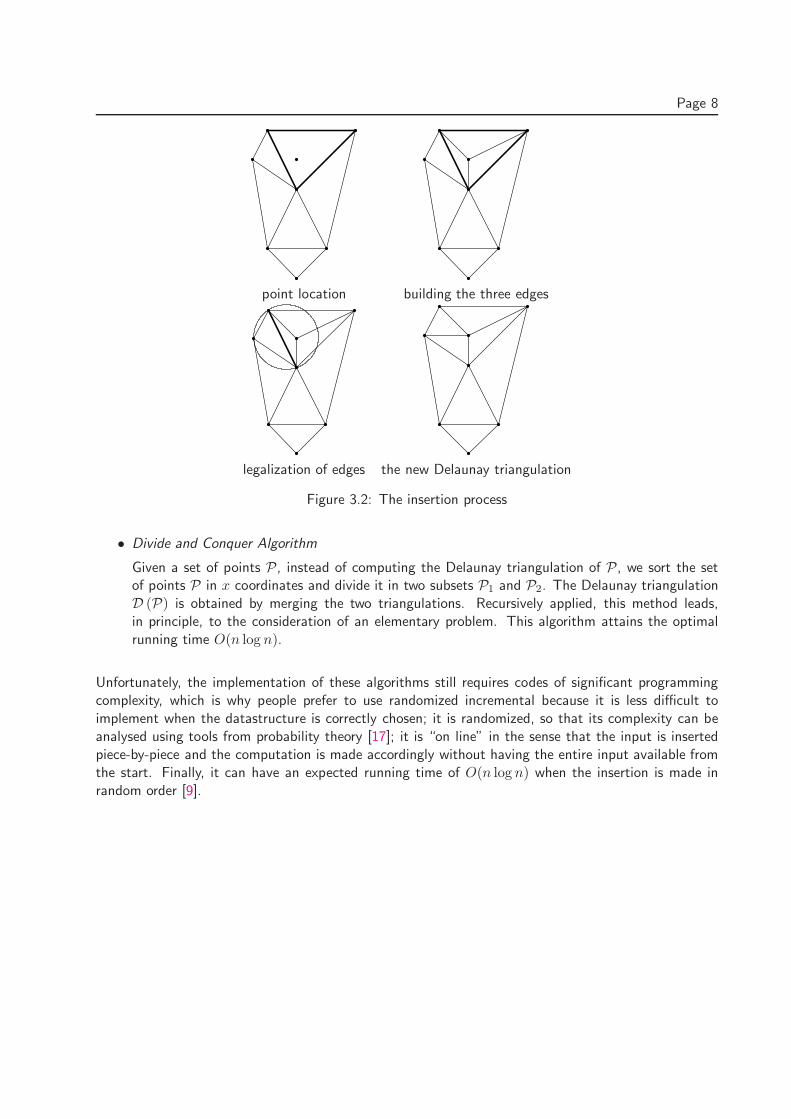
Let P be a set of points in the plane and D (Pr) a triangulation of Pr ⊂ P at stage r. The triangulationD (Pr+1) is obtained by inserting a point pr, randomly taken from P \ Pr, in D (Pr). The algorithmlocates pr using a DAG for point location based on the history of the Delaunay triangulation called theDelaunay tree (Section 4.2). At this stage two cases can happen: either the point lies on an edge orstrictly inside the triangle. In the first case, we construct two edges connecting pr to the vertices ofthe two adjacent triangles, whereas in the second case, we construct three edges connecting the pointand the three vertices of the triangle (Figure 3.1) . Since we look for a legal triangulation, we check ifevery edge of the containing triangle is valid with respect to the empty circle criterion. We then proceedrecursively until all the points are inserted. At last, we get the Delaunay triangulation of P. Figure 3.2shows the insertion process.

pl

pj

pk

pi

pr

pi

pj

pk

pr

Figure 3.1: Two cases of the positions of pr

3.0.2 Why Randomized Incremental Algorithm?

Interesting algorithms have been implemented. The most remarquable of them are:

• Plane Sweep Algorithm

In 1985, Fortune invented a clever Plane Sweep algorithm which attains the optimal boundO(n log n). Plane-sweep algorithms pass a sweep line over the plane, leaving at any time theproblem solved for the portion of the plane already swept and unsolved for the portion not yetreached. A plane-sweep algorithm for the Voronoi diagram would have the diagram constructedbehind the line. It seems quite impossible, as Voronoi edges of a Voronoi region V(p) would beencountered by the sweep line L before L encounters the site p responsible for the region. Fortunesurmounted this seeming impossibility by an extraordinary clever idea [15].

7

point location building the three edges

legalization of edges the new Delaunay triangulation

Figure 3.2: The insertion process

• Divide and Conquer Algorithm

Given a set of points P, instead of computing the Delaunay triangulation of P, we sort the setof points P in x coordinates and divide it in two subsets P1 and P2. The Delaunay triangulationD (P) is obtained by merging the two triangulations. Recursively applied, this method leads,in principle, to the consideration of an elementary problem. This algorithm attains the optimalrunning time O(n log n).

Unfortunately, the implementation of these algorithms still requires codes of significant programmingcomplexity, which is why people prefer to use randomized incremental because it is less difficult toimplement when the datastructure is correctly chosen; it is randomized, so that its complexity can beanalysed using tools from probability theory [17]; it is “on line” in the sense that the input is insertedpiece-by-piece and the computation is made accordingly without having the entire input available fromthe start. Finally, it can have an expected running time of O(n log n) when the insertion is made inrandom order [9].

4. Computation of the Delaunay Triangulation

We have now enough information to build the algorithm. We proceed in four phases. We first start withthe initialisation of three dummy points which enclose all the points of P; we then describe an efficientlocation technique to locate queries; we next discuss the Legalization which is a procedure verifyingthe empty circle criterion; and finally, give pseudo-code of the algorithm. The last section contains theanalysis of the algorithm

4.1 Initialisation of the Three Dummy Points

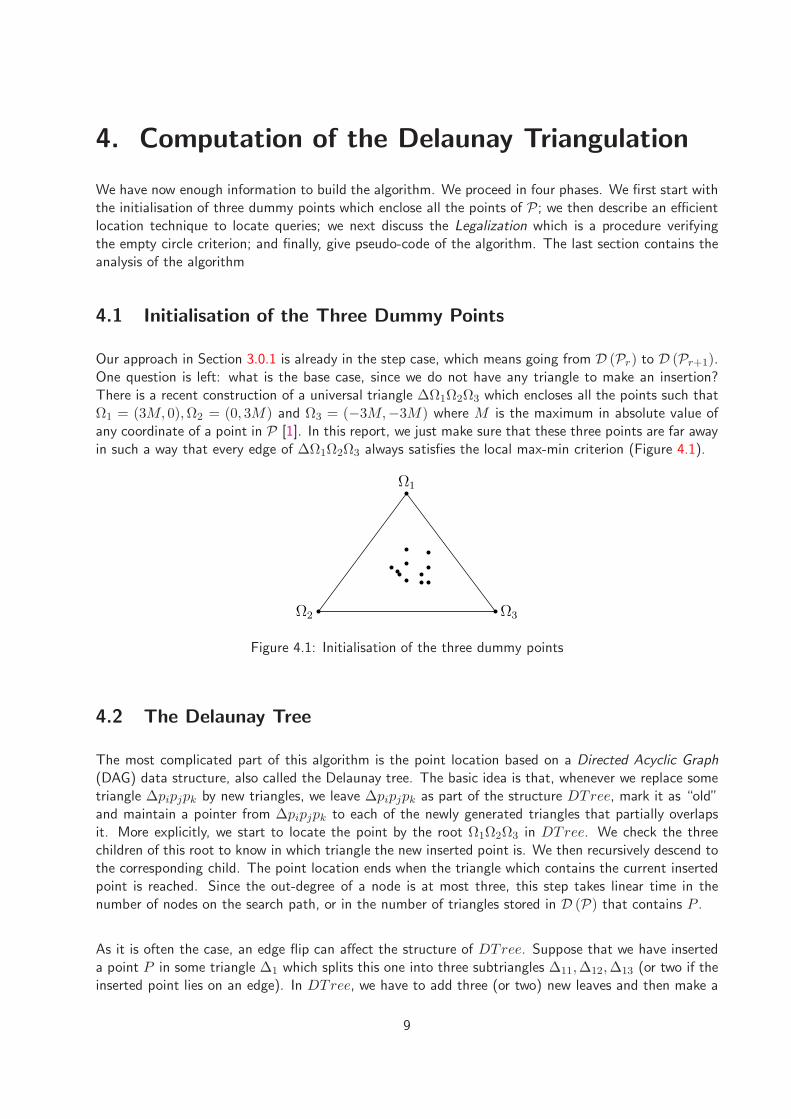
Our approach in Section 3.0.1 is already in the step case, which means going from D (Pr) to D (Pr+1).One question is left: what is the base case, since we do not have any triangle to make an insertion?There is a recent construction of a universal triangle ∆Ω1Ω2Ω3 which encloses all the points such thatΩ1 = (3M, 0),Ω2 = (0, 3M) and Ω3 = (−3M,−3M) where M is the maximum in absolute value ofany coordinate of a point in P [1]. In this report, we just make sure that these three points are far awayin such a way that every edge of ∆Ω1Ω2Ω3 always satisfies the local max-min criterion (Figure 4.1).

Ω1

Ω2 Ω3

Figure 4.1: Initialisation of the three dummy points

4.2 The Delaunay Tree

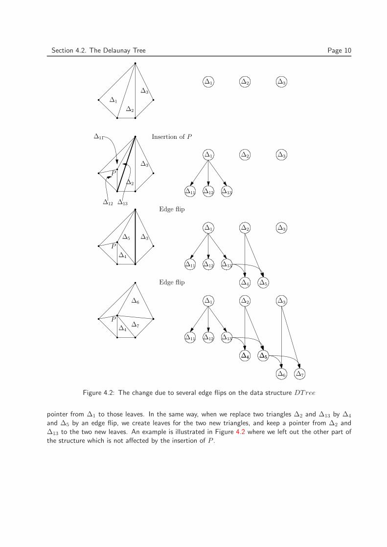
The most complicated part of this algorithm is the point location based on a Directed Acyclic Graph(DAG) data structure, also called the Delaunay tree. The basic idea is that, whenever we replace sometriangle ∆pipjpk by new triangles, we leave ∆pipjpk as part of the structure DTree, mark it as “old”and maintain a pointer from ∆pipjpk to each of the newly generated triangles that partially overlapsit. More explicitly, we start to locate the point by the root Ω1Ω2Ω3 in DTree. We check the threechildren of this root to know in which triangle the new inserted point is. We then recursively descend tothe corresponding child. The point location ends when the triangle which contains the current insertedpoint is reached. Since the out-degree of a node is at most three, this step takes linear time in thenumber of nodes on the search path, or in the number of triangles stored in D (P) that contains P .

As it is often the case, an edge flip can affect the structure of DTree. Suppose that we have inserteda point P in some triangle ∆1 which splits this one into three subtriangles ∆11,∆12,∆13 (or two if theinserted point lies on an edge). In DTree, we have to add three (or two) new leaves and then make a

9

Section 4.2. The Delaunay Tree Page 10

∆1

∆2

∆3

P

∆2

∆3

∆11

∆12 ∆13

P

∆4

∆3∆5

P

∆4

∆7

∆6

∆1 ∆2 ∆3

∆1 ∆2 ∆3

∆1 ∆2 ∆3

∆1 ∆2 ∆3

∆11 ∆12 ∆13

∆11 ∆12 ∆13

∆11 ∆12 ∆13

∆4 ∆5

∆4 ∆5

∆6 ∆7

∆4 ∆5

Insertion of P

Edge flip

Edge flip

Figure 4.2: The change due to several edge flips on the data structure DTree

pointer from ∆1 to those leaves. In the same way, when we replace two triangles ∆2 and ∆13 by ∆4

and ∆5 by an edge flip, we create leaves for the two new triangles, and keep a pointer from ∆2 and∆13 to the two new leaves. An example is illustrated in Figure 4.2 where we left out the other part ofthe structure which is not affected by the insertion of P .

Section 4.3. Legalization Page 11

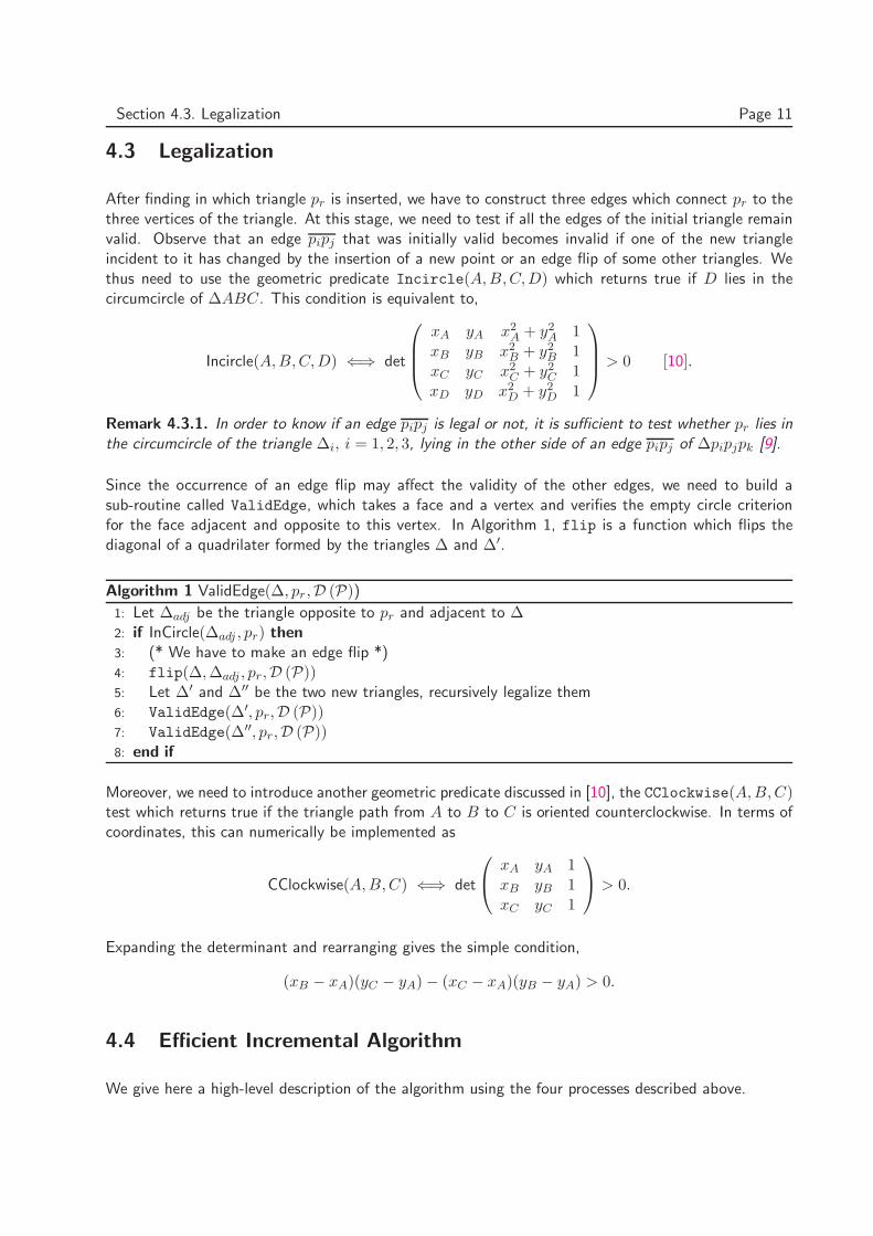
4.3 Legalization

After finding in which triangle pr is inserted, we have to construct three edges which connect pr to thethree vertices of the triangle. At this stage, we need to test if all the edges of the initial triangle remainvalid. Observe that an edge pipj that was initially valid becomes invalid if one of the new triangleincident to it has changed by the insertion of a new point or an edge flip of some other triangles. Wethus need to use the geometric predicate Incircle(A,B,C,D) which returns true if D lies in thecircumcircle of ∆ABC. This condition is equivalent to,

Incircle(A,B,C,D) ⇐⇒ det

xA yA x2A + y2

A 1xB yB x2

B + y2B 1

xC yC x2C + y2

C 1xD yD x2

D + y2D 1

> 0 [10].

Remark 4.3.1. In order to know if an edge pipj is legal or not, it is sufficient to test whether pr lies inthe circumcircle of the triangle ∆i, i = 1, 2, 3, lying in the other side of an edge pipj of ∆pipjpk [9].

Since the occurrence of an edge flip may affect the validity of the other edges, we need to build asub-routine called ValidEdge, which takes a face and a vertex and verifies the empty circle criterionfor the face adjacent and opposite to this vertex. In Algorithm 1, flip is a function which flips thediagonal of a quadrilater formed by the triangles ∆ and ∆′.

Algorithm 1 ValidEdge(∆, pr,D (P))

1: Let ∆adj be the triangle opposite to pr and adjacent to ∆2: if InCircle(∆adj , pr) then

3: (* We have to make an edge flip *)4: flip(∆,∆adj , pr,D (P))5: Let ∆′ and ∆′′ be the two new triangles, recursively legalize them6: ValidEdge(∆′, pr,D (P))7: ValidEdge(∆′′, pr,D (P))8: end if

Moreover, we need to introduce another geometric predicate discussed in [10], the CClockwise(A,B,C)test which returns true if the triangle path from A to B to C is oriented counterclockwise. In terms ofcoordinates, this can numerically be implemented as

CClockwise(A,B,C) ⇐⇒ det

xA yA 1xB yB 1xC yC 1

> 0.

Expanding the determinant and rearranging gives the simple condition,

(xB − xA)(yC − yA)− (xC − xA)(yB − yA) > 0.

4.4 Efficient Incremental Algorithm

We give here a high-level description of the algorithm using the four processes described above.

Section 4.5. Correctness and Efficiency Page 12

Algorithm 2 Delaunay Triangulation of P

Input: A set P of n + 1 points in the planeOutput: A Delaunay triangulation of P1: Initialise the triangulation D (P) to be Ω1Ω2Ω3

2: Make a random permutation [p1, p2, p3, . . . , pn] of P3: for r ← 1 to n do

4: (* Take the point pr which should not be already selected *)5: Find a triangle ∆ which contains pr

6: if If pr lies in the interior of ∆ then

7: Divide ∆ to ∆1,∆2 and ∆3

8: (* Check for the validity of edges *)9: ValidEdge(∆1, pr,D (P))

10: ValidEdge(∆2, pr,D (P))11: ValidEdge(∆3, pr,D (P))12: else

13: (*pr lies on an edge e of ∆*)14: Let ∆′ be the triangle sharing the edge e with ∆, then divide ∆′to ∆′

1,∆′2 and ∆ to ∆1,∆2

15: (* Check for validity of edges *)16: ValidEdge(∆′

1, pr,D (P))17: ValidEdge(∆′

2, pr,D (P))18: ValidEdge(∆1, pr,D (P))19: ValidEdge(∆2, pr,D (P))20: end if

21: end for

22: Delete all triangles containing Ω1, Ω2 or Ω3 as vertices from D (P)23: return D (P)

4.5 Correctness and Efficiency

The goal of this section is to prove that the Delaunay triangulation of a set of planar points constructedwith the incremental randomized algorithm can be computed in O(n log n) expected time and O(n)expected storage. Before starting, let Pr := p1, . . . , pr be the set of points already inserted at thestage r which contains r elements and D (Pr) := D(Ω0,Ω1,Ω2 ∪ Pr) the corresponding Delaunaytriangulation.

Lemma 4.5.1. (General results)

1. Let P be a set of n points in the plane which are not all collinear, and let k denote the numberof points in P that lie on the boundary of the convex hull of P . Then any triangulation of P has2n− 2− k triangles and 3n − 3− k edges.

2. For n ≥ 3, the number of vertices in the Voronoi diagram of a set of n point sites in the plane isat most 2n− 5 and the number of edges is at most 3n− 6.

Proof. The proof is not complicated, but quite long, using some results from graph theory. For moredetails, we refer to [1].

Lemma 4.5.2. The expected degree of a random point of Pr is at most 6.


Proof. Let deg(pr,D (Pr)) be the degree of pr in D (Pr). For the moment, we fixe the set Pr andmake backwards analysis. It follows from the second result of Lemma 4.5.1 that D (Pr) has at most3(r+3)−6 edges, where the extra three edges come from the initial triangle Ω1Ω2Ω3, and therefore, theHandshake Lemma 1 implies that the total degree of the vertices in Pr is less than 2[3(r +3)− 9] = 6r.We deduce that the expected degree of a random point of Pr is at most 6.

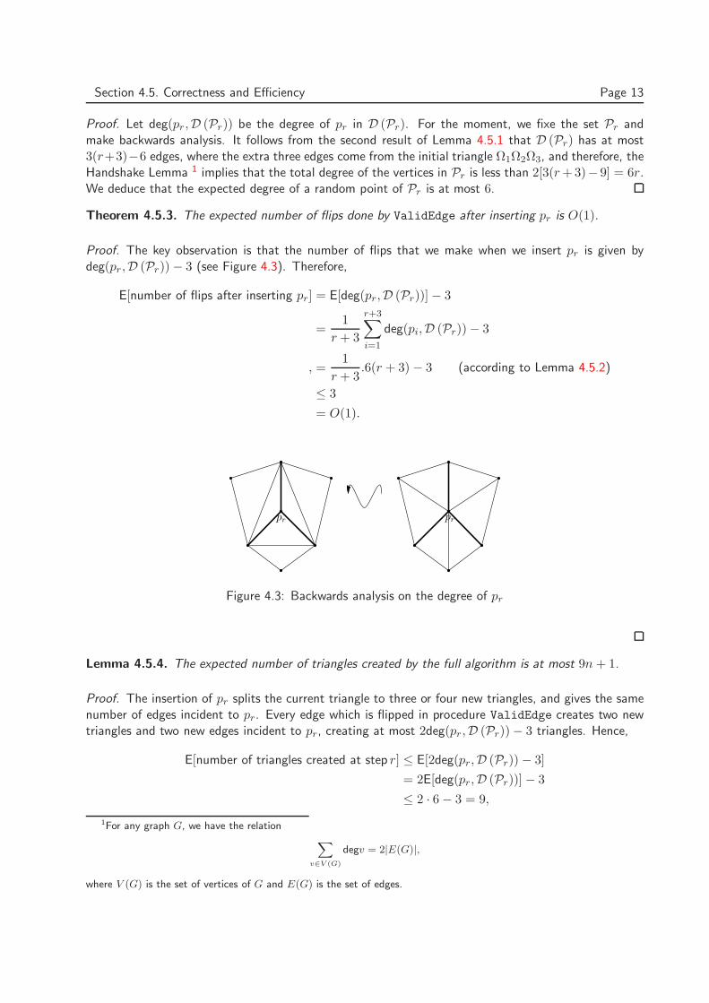
Theorem 4.5.3. The expected number of flips done by ValidEdge after inserting pr is O(1).

Proof. The key observation is that the number of flips that we make when we insert pr is given bydeg(pr,D (Pr))− 3 (see Figure 4.3). Therefore,

E[number of flips after inserting pr] = E[deg(pr,D (Pr))]− 3

=1

r + 3

r+3∑

i=1

deg(pi,D (Pr))− 3

, =1

r + 3.6(r + 3) − 3 (according to Lemma 4.5.2)

≤ 3

= O(1).

pr pr

Figure 4.3: Backwards analysis on the degree of pr

Lemma 4.5.4. The expected number of triangles created by the full algorithm is at most 9n + 1.

Proof. The insertion of pr splits the current triangle to three or four new triangles, and gives the samenumber of edges incident to pr. Every edge which is flipped in procedure ValidEdge creates two newtriangles and two new edges incident to pr, creating at most 2deg(pr,D (Pr))− 3 triangles. Hence,

E[number of triangles created at step r] ≤ E[2deg(pr,D (Pr))− 3]

= 2E[deg(pr,D (Pr))]− 3

≤ 2 · 6− 3 = 9,

1For any graph G, we have the relation

X

v∈V (G)

degv = 2|E(G)|,

where V (G) is the set of vertices of G and E(G) is the set of edges.


having also used Lemma 4.5.2.

The desired result is then obtained by summing over r and using the linearity of the expectation andthen adding the initial triangle Ω1Ω2Ω3.

Definition 4.5.5. The scope of a triangle is defined in [9] to be the number of sites contained in theinterior of its circumcircle. The scope of a triangle can assume values between 0 and n−3, and triangleswith zero scope are the Delaunay triangles.

Lemma 4.5.6. [9] Let ∆pipjpk be a triangle with scope k. Then the probability that ∆2 appears as aDelaunay triangle during the incremental construction is given by

Proba(∆ appears as Delaunay triangle) =6

(k + 1)(k + 2)(k + 3). (4.1)

Proof. The only possibility for ∆ to be Delaunay is that pi, pj and pk are inserted first before any of thek sites inside its circumcircle. This condition is equivalent to compute the event E:“insert pi, pj and pk

first (without any order) and independently on the time of insertion of the sites of its scope”. Hence,

Proba(E) =3!k!

(k + 3)!=

6

(k + 1)(k + 2)(k + 3).

We next introduce the new variable Tl defined to be the set of triangles ∆pipjpk whose scope is l, andwe use the notation T≤m =

⋃md=0 Td.

Lemma 4.5.7. [9] The number of triangles ∆pipjpk whose scope is m is

‖T≤m‖ = O(n(m + 1)2). (4.2)

Proof. This proof is an extended version of the one presented in [9] but the probabilistic technique isfrom Clarkson and Shor [17]. The idea is to take a random sample R of size r (r ≥ 3) among the givensites, and denote by D (R) the set of Delaunay triangles formed by this sample. The expected numberof such triangles is thus

E [‖D (R) ‖] =∑

∆

Proba(∆ ∈ D (R))

=

n−3∑

l=0

∑

∆∈Tl

Proba(∆ ∈ D (R))

≥m

∑

l=0

∑

∆∈Tl

Proba(∆ ∈ D (R)).

A necessary condition for ∆pipjpk to be in D (R) is that pi, pj , pk ∈ R, where as a sufficient conditionis that none of the l sites in the interior of its circumcircle is in R. Denoting this event as F, we have

Proba(F ) =

( r−3

n−j−3

)

(rn

) ≥

( r−3

n−k−3

)

(rn

) for j ≤ k.

2Here, the triangle ∆ has pi, pj and pk as vertices but we use this notation for simplicity


Since ‖D (R) ‖ is at most 2r (first result of Lemma 4.5.1), we obtain

2r ≥ E [‖D (R) ‖] ≥

k∑

l=0

‖Tl‖.

(

r−3

n−k−3

)

(

rn

) ,

which amounts to

‖T≤k‖ ≤2r

(rn

)

(

r−3

n−k−3

) =2n

(

r−1

n−1

)

(

r−3

n−k−3

) = 2nB(n− 1, k + 2, r − 3, 2),

where

B(N,M, s, t) =

(

s+tN

)

( sN−M

) .

In order to obtain the best upper bound, we have to minimise B(n− 1, k + 2, r − 3, 2) with respect tor. In general, we have for successive values of s the ratio [9].

B(N,M, s + 1, t)/B(N,M, s, t) = t(N −M + 1)/M.

Hence, the minimum of B(N,M, s, t) for fixed N,M and t occurs when s = [t(N −M + 1)/M ].

In our case, the function B is minimised when

r = [2n/(k + 2)] + 1. (4.3)

Now,

B(n− 1, k + 2, r − 3, 2) =n− 1

r − 1·n− 2

r − 2·n− 3

n− r·

n− 4

n− r − 1· · · · ·

n− k − 2

n− r − k + 1.

Observing that

n− 1

r − 1<

n− 2

r − 2, r < n

fracn− in− (r + i− 3) ≤n− k − 2

n− r − k + 1, 3 ≤ i ≤ k + 2,

we find

B(n− 1, k + 2, r − 3, 2) <

(

n− 2

r − 1

)2 (

n− k − 2

n− r − k + 1

)k

.

Using the minimum value r in (4.3), we obtain

B(n− 1, k + 2, r − 3, 2) <

(

(n + 2)(k + 2)

2n − 2k − 4

)2 (

1 +2

k

)k

<

(

n− 2

2

)2

(k + 2)2(

1 +2

k

)k

= O((k + 1)2),

having also used the fact that k ≤ n− 3.


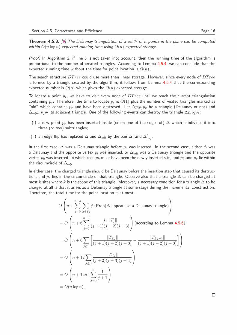
Theorem 4.5.8. [9] The Delaunay triangulation of a set P of n points in the plane can be computedwithin O(n log n) expected running time using O(n) expected storage.

Proof. In Algorithm 2, if line 5 is not taken into account, then the running time of the algorithm isproportional to the number of created triangles. According to Lemma 4.5.4, we can conclude that theexpected running time without the time for point location is O(n).

The search structure DTree could use more than linear storage. However, since every node of DTreeis formed by a triangle created by the algorithm, it follows from Lemma 4.5.4 that the correspondingexpected number is O(n) which gives the O(n) expected storage.

To locate a point pr, we have to visit every node of DTree until we reach the current triangulationcontaining pr. Therefore, the time to locate pr is O(1) plus the number of visited triangles marked as“old” which contains pr and have been destroyed. Let ∆pipjpk be a triangle (Delaunay or not) and∆adjpipjpl its adjacent triangle. One of the following events can destroy the triangle ∆pipjpk:

(i) a new point pr has been inserted inside (or on one of the edges of) ∆ which subdivides it intothree (or two) subtriangles;

(ii) an edge flip has replaced ∆ and ∆adj by the pair ∆′ and ∆′adj .

In the first case, ∆ was a Delaunay triangle before pr was inserted. In the second case, either ∆ wasa Delaunay and the opposite vertex pl was inserted, or ∆adj was a Delaunay triangle and the oppositevertex pk was inserted, in which case pk must have been the newly inserted site, and pk and pr lie withinthe circumcircle of ∆adj .

In either case, the charged triangle should be Delaunay before the insertion step that caused its destruc-tion, and pr lies in the circumcircle of that triangle. Observe also that a triangle ∆ can be charged atmost k sites where k is the scope of this triangle. Moreover, a necessary condition for a triangle ∆ to becharged at all is that it arises as a Delaunay triangle at some stage during the incremental construction.Therefore, the total time for the point location is at most,

O

n +n−3∑

j=0

∑

∆∈Tj

j · Prob(∆ appears as a Delaunay triangle)

= O

n + 6

n−3∑

j=0

j · ‖Tj‖

(j + 1)(j + 2)(j + 3)

(according to Lemma 4.5.6)

= O

n + 6∑

j≥0

[

‖T≤j‖

(j + 1)(j + 2)(j + 3)−

‖T≤j−1‖

(j + 1)(j + 2)(j + 3)

]

= O

n + 12∑

j≥0

‖T≤j‖

(j + 2)(j + 3)(j + 4)

= O

n + 12n ·

n∑

j=0

1

j + 1

= O(n log n).


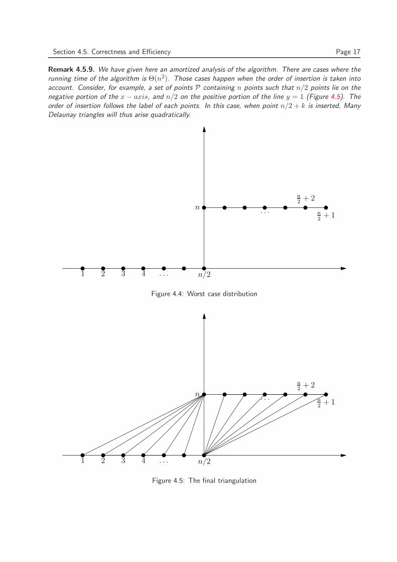
Remark 4.5.9. We have given here an amortized analysis of the algorithm. There are cases where therunning time of the algorithm is Θ(n2). Those cases happen when the order of insertion is taken intoaccount. Consider, for example, a set of points P containing n points such that n/2 points lie on thenegative portion of the x− axis, and n/2 on the positive portion of the line y = 1 (Figure 4.5). Theorder of insertion follows the label of each points. In this case, when point n/2 + k is inserted, ManyDelaunay triangles will thus arise quadratically.

n/21 2 3 4 . . .

nn2

+ 1

n2

+ 2

. . .

Figure 4.4: Worst case distribution

n/21 2 3 4 . . .

nn2

+ 1

n2

+ 2

. . .

Figure 4.5: The final triangulation

5. Applications

The implementation of such optimal algorithms are quite complicated and need a considerable amountof lines of code. Since the edge flips can be done in O(1) time (Theorem 4.5.3), we can, at least,test the speed of the Delaunay tree point location without this procedure. Some results on differentprove that the implementation gives good results even for huge number of points. We have chosenthe vertices-and-faces-based datastructure of CGAL-python. The last part will introduce the concept ofterrain modelling.

5.0.1 Vertices-and-Faces-Based Datastructure

The implementation is made with CGAL-Python (http://cgal-python.gforge.inria.fr/) usingvertices-and-faces-based datastructure. There are other structures which are standard in the field ofcomputational geometry such as the quad-edge data structure of Guibas and Stolfi [10] or the doubly-connected edge list of Muller and Preparata [3]. However, our choice of CGAL is because it can be usedwith Python and the vertices-and-faces-based datastructure is easy to manipulate.

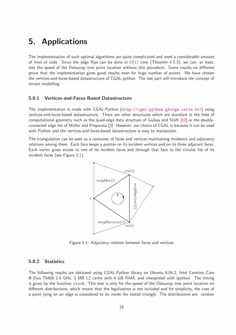
The triangulation can be seen as a container of faces and vertices maintaining incidence and adjacencyrelations among them. Each face keeps a pointer on its incident vertices and on its three adjacent faces.Each vertex gives access to one of its incident faces and through that face to the circular list of itsincident faces (see Figure 5.1).

f

i

cw(i)

ccw(i)

neighbor(i)

neighbor(ccw(i))

neig

hbo

r(cw(i))

Figure 5.1: Adjacency relation between faces and vertices

5.0.2 Statistics

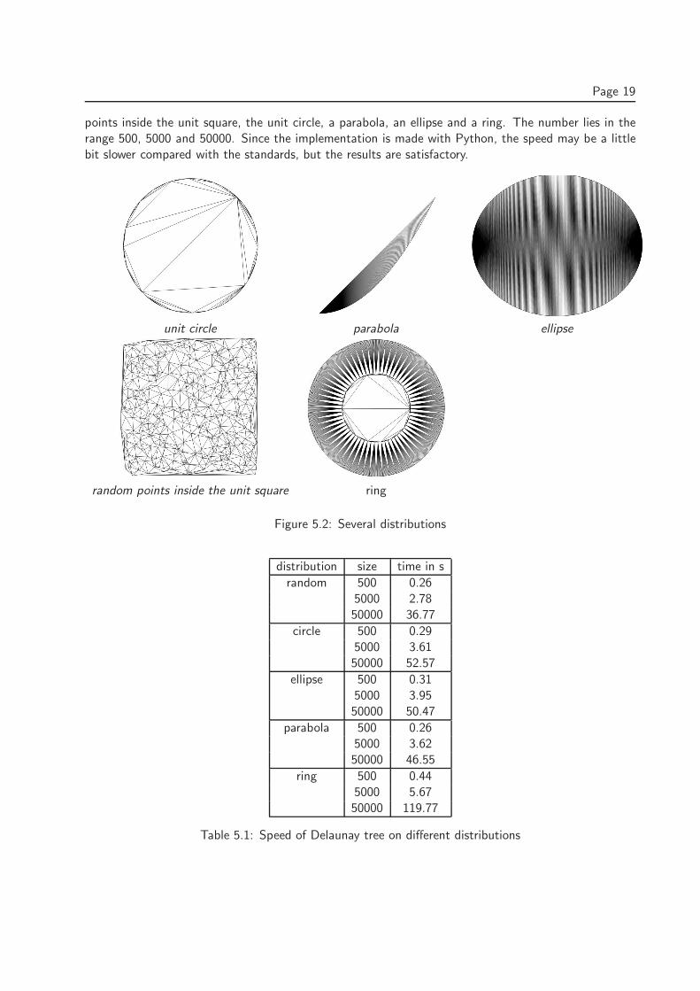
The following results are obtained using CGAL-Python library on Ubuntu 8.04.2, Intel Centrino Core@ Duo T6400 2.0 GHz, 2 MB L2 cache with 4 GB RAM, and interpreted with Ipython. The timingis given by the function clock. This test is only for the speed of the Delaunay tree point location ondifferent distributions, which means that the legalization is not included and for simplicity, the case ofa point lying on an edge is considered to be inside the tested triangle. The distributions are: random

18

http://cgal-python.gforge.inria.fr/

points inside the unit square, the unit circle, a parabola, an ellipse and a ring. The number lies in therange 500, 5000 and 50000. Since the implementation is made with Python, the speed may be a littlebit slower compared with the standards, but the results are satisfactory.

unit circle parabola ellipse

random points inside the unit square ring

Figure 5.2: Several distributions

distribution size time in s

random 500 0.265000 2.7850000 36.77

circle 500 0.295000 3.6150000 52.57

ellipse 500 0.315000 3.9550000 50.47

parabola 500 0.265000 3.6250000 46.55

ring 500 0.445000 5.6750000 119.77

Table 5.1: Speed of Delaunay tree on different distributions

Section 5.1. Terrain Generation Page 20

5.1 Terrain Generation

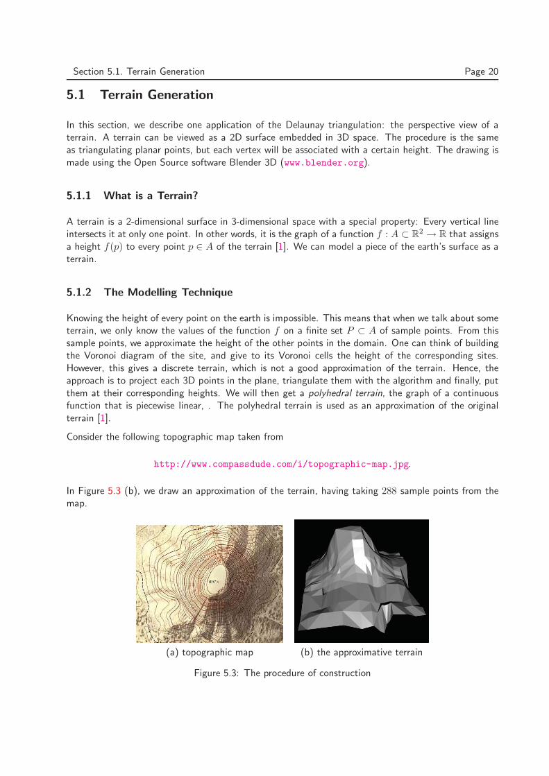
In this section, we describe one application of the Delaunay triangulation: the perspective view of aterrain. A terrain can be viewed as a 2D surface embedded in 3D space. The procedure is the sameas triangulating planar points, but each vertex will be associated with a certain height. The drawing ismade using the Open Source software Blender 3D (www.blender.org).

5.1.1 What is a Terrain?

A terrain is a 2-dimensional surface in 3-dimensional space with a special property: Every vertical lineintersects it at only one point. In other words, it is the graph of a function f : A ⊂ R

2 → R that assignsa height f(p) to every point p ∈ A of the terrain [1]. We can model a piece of the earth’s surface as aterrain.

5.1.2 The Modelling Technique

Knowing the height of every point on the earth is impossible. This means that when we talk about someterrain, we only know the values of the function f on a finite set P ⊂ A of sample points. From thissample points, we approximate the height of the other points in the domain. One can think of buildingthe Voronoi diagram of the site, and give to its Voronoi cells the height of the corresponding sites.However, this gives a discrete terrain, which is not a good approximation of the terrain. Hence, theapproach is to project each 3D points in the plane, triangulate them with the algorithm and finally, putthem at their corresponding heights. We will then get a polyhedral terrain, the graph of a continuousfunction that is piecewise linear, . The polyhedral terrain is used as an approximation of the originalterrain [1].

Consider the following topographic map taken from

http://www.compassdude.com/i/topographic-map.jpg.

In Figure 5.3 (b), we draw an approximation of the terrain, having taking 288 sample points from themap.

(a) topographic map (b) the approximative terrain

Figure 5.3: The procedure of construction

www.blender.org

http://www.compassdude.com/i/topographic-map.jpg


Note that the quality of the approximation is proportional to the number of the sample points. Unfor-tunately, taking several samples points is costly and not very helpful for those in game programmingwhere generation of terrain should be fast and of good quality. This observation lead to the idea ofcreating a terrain generator. We will next present a recent technique to generate them.

5.1.3 The Terrain Generator

5.1.4 Main Idea

The generation of the terrain is based on a very clever idea, where mountains are represented by thetwo dimensional gaussian,

f(x, y) = (−1)M × exp(−σx(x− µx)2 − σy(y − µy)2). (5.1)

Here,

• M is a boolean which decides if the surface is a valley or a mountain;

• h is the height of the mountain;

• σx, σy define how spread out the mountain is (it can be interpreted as the inverse of the variancein statistics).

• µx, µy is the centre of the mountain (it is the mean value in statistics);

5.1.5 The Process of Construction

We have built a class called Terrain which gives access to the following variables:

nb_centre: the number of mountains and valleys;

centre: array of two rows which defines the coordinate of each mountain;

etal: array of two rows which defines how spread out each mountain should be;

height: vector which defines the height of each mountain.

mountain: vector formed by booleans

The initial terrain is initialised by the function Terrain_init which takes as inputnb_centre andthe dimension of the grid point xmin,xmax,ymin,ymax. It returns an initialisation of the terrainby assigning random positions and random heights to each mountain. We then use the functionMountain_construct which takes an initialised terrain and returns the final terrain by replacing eachmountain by the two dimensional gaussian .

At this stage, each point of the terrain is represented by three coordinates noted (x, y, h) where h isa function of (x, y) generated by Mountain_construct. The user defines how many sample pointshave to be taken for the triangulation. We do not use any location structure, instead we look for thetriangle with the bigger area and insert the point in the centroid of this triangle. Thus the running time


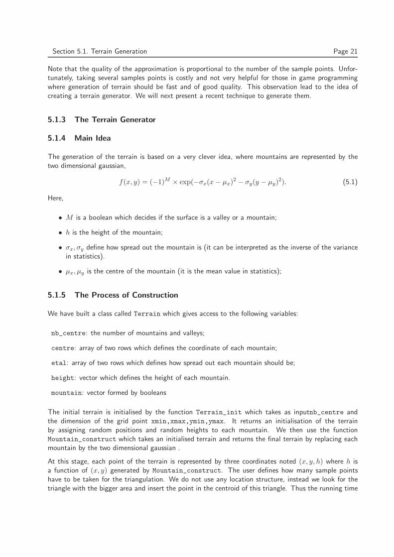
of locating the triangle and inserting the point is O(1) when the list of triangles are sorted (in terms ofarea) in decreased order. The sorting takes O(n) which gives an O(n2) of the total algorithm. Of coursewe can use a location structure but the quality of the triangulation is better with the centroid technique[19]. In Figure 5.4 (a), we triangulate a grid of 16 points, the same triangulation is done ni (b), but usingthe centroid technique. The advantage of (b) is that there are triangles which minimum angle is less than45 . Note that at the beginning, we already have a triangulation formed by xmin,xmax,ymin,ymax,

(a) grid points (b) centroid technique

Figure 5.4: Quality of triangulation

so that we start the locating process with them. We can summarise the process by the followingpseudo-code

Algorithm 3 Terrain Generation

Input: xmin,xmax,ymin,ymax,nb_centre,the number of sample points nOutput: Perspective view of a generated terrain1: Initialise the terrain with Terrain_init

2: Let DT be the Delaunay triangulation formed by xmin,xmax,ymin,ymax

3: (*Construct the triangulation of the rectangle formed by xmin,xmax,ymin,ymax,nb_centre*)4: for r ← 1 to n do

5: for each face of DT do

6: Take the one which has the maximum area7: end for

8: (*Let f be this face*)9: Compute the centroid P of f

10: Use the process from line 6 to line 11 in Algorithm 2 with P and f11: end for

12: Give a height to its point of DT by Mountain_construct

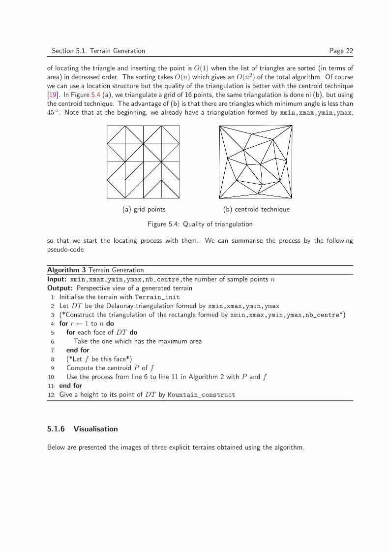
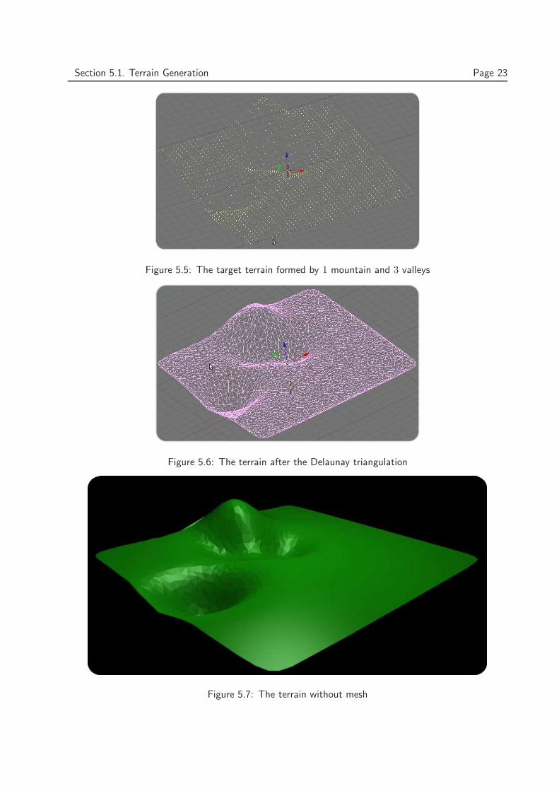
5.1.6 Visualisation

Below are presented the images of three explicit terrains obtained using the algorithm.


Figure 5.5: The target terrain formed by 1 mountain and 3 valleys

Figure 5.6: The terrain after the Delaunay triangulation

Figure 5.7: The terrain without mesh


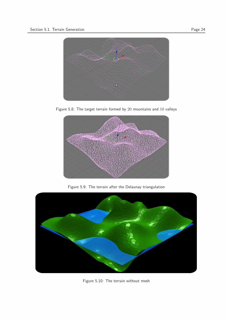
Figure 5.8: The target terrain formed by 20 mountains and 10 valleys


Figure 5.10: The terrain without mesh


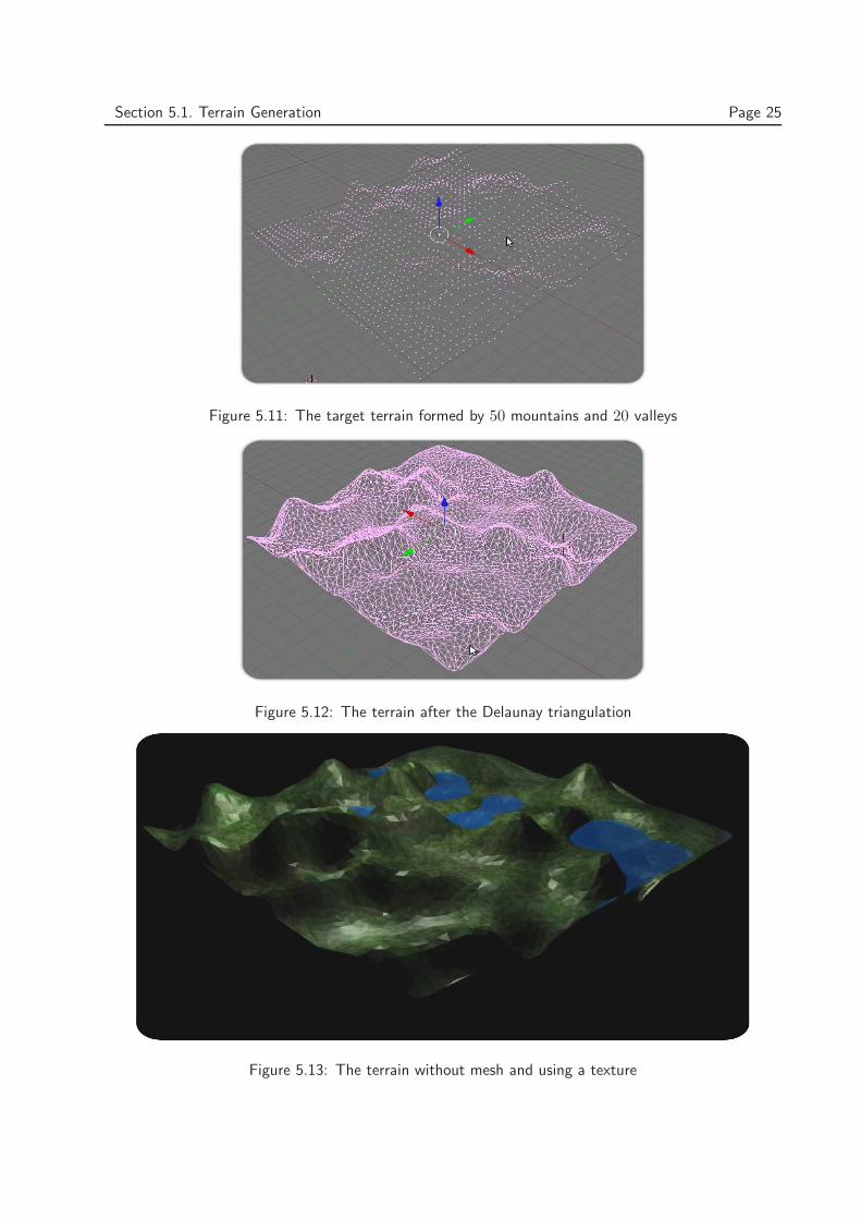
Figure 5.11: The target terrain formed by 50 mountains and 20 valleys


Figure 5.13: The terrain without mesh and using a texture

6. Notes and Comments

There are several applications of the Delaunay triangulation which are well known outside the field ofcomputational geometry. Triangulations are used in finite element methods [8], in computer graphics,in image morphing [18] and many more. The randomized incremental algorithm that we have givenhere is due to Guibas et al. [9], but the analysis of the expected storage has been simplified and thealgorithm implemented and tested. The Delaunay tree is not the fastest point location in the classof randomized incremental algorithms. Recently, Olivier Delliers [4] has proposed a new datastructurecalled the Delaunay hierarchy which is based on the nearest neighbor paradigm and uses only 3% memoryduring the point location compared to the one presented here. Nowadays, the triangulations of a set ofpoints are not sufficient, the reality implies introducing constraints in the input data which are edgesand holes. Sometimes, triangulating a set of points with small angles are difficult to obtain in termsof quality, so that extra points, called Steiner points, are added during the triangulation. These newconsiderations introduce us to the concept of high order constrained Delaunay triangulation which isstill a very active area of research in computational geometry.

The terrain generator is based on the idea of Jean Claude Isenman [12] with certain translations intoPython. Generating a terrain is one part of the work, yet there are a lot of details to modelise, muchmore imagination to explore. The research will never end up as long as it imitates the reality, which isthe main objective .

All the codes of this project are accessible at

http://users.aims.ac.za/~faniry/essayproject.html,

where they can be used freely under the GNU General Public Licence as published by the Free SoftwareFoundation.

26

http://users.aims.ac.za/~faniry/essayproject.html

Acknowledgements

This work would have never been achieved without the contribution of Lord Jesus Christ the Son ofGod, the valuable criticisms of my supervisor Dr Jeff W Sanders, the discussions with my tutor MiangalyGaelle Andriamaro, the assistance of my family and the encouragement of my AIMS colleagues. I wouldhave not bee able to study at AIMS without the help of Gerard Razafimanantsoa. Finally, I would liketo say well done to the AIMS staff for the great project that they are executing.

27

References

[1] de Berg, M., van Kreveld, M., Overmars, M., and Schwarzkopf, O. ComputationalGeometry: Algorithms and Applications. Springer, 2000.

[2] Delone, B. N. Sur la sphere vide. Bul. Acad. Sci. URSS, Class. Sci. Nat. (1934), 793–800.

[3] D.E.Muller, and Preparata, F. Finding the intersection of two convex polyhedra. Theoritic.Comput. Sci 7 (1978), 217–236.

[4] Devillers, O. The Delaunay Hierarchy. Internat. J.Found. Comput. Sci. 13 (2002), 163–180.

[5] Edelsbrunner, H. Algorithms in Combinatorial Geometry. Springer-Verlag, 1987.

[6] E.P., M., and I. Saias I., Z. B. Fast Randomized Point Location Without Preprocessingin Two- and Three-dimensional Delaunay Triangulations. CompGeom’96, Philadelphia (1996),274–283.

[7] Fortune, S. A sweepline algorithm for the Voronoi diagrams. Algorithmica 2 (1987), 153–174.

[8] George, P.-L., and Borouchaki, H. Delaunay triangulation and Meshing: application tofinite elements. HERMES, 1998.

[9] Guibas, L. J., Knuth, D. E., and Sharir, M. Randomized Incremental Construction ofDelaunay and Voronoi Diagrams. Algorithmica 7 (1992), 381–413.

[10] Guibas, L. J., and Stolfi, J. Primitives for the manipulation of general subdivisions and thecomputation of Voronoi diagrams. ACM Trans. Graphics 4 (1985), 74–123.

[11] INRIA. http://cgal-python.gforge.inria.fr/. Computational Geometry Algorithm for Python.

[12] Isenmann, J. C. B. B. Generation de terrain et triangulation de Delaunay.http://fearyourself.developpez.com/tutoriel/jeu/Delaunay/ (2006).

[13] Lecky-Thompson, and Guy W. Real-Time Realistic Terrain Generation. Game ProgrammingGems (2000), 484–498.

[14] Okabe, A., Boots, B., Sugihara, K., and Chiu, S. N. Spatial Tessellations: Conceptsand Applications of Voronoi Diagrams. Wiley, 2000.

[15] O’Rourke, J. Computational Geometry in C: Second Edition. Cambridge University Press, 1998.

[16] Shankel, and Jason. Fractal Terrain Generation. Game Programming Gems (2000), 499–511.

[17] Teillaud, M. Towards Dynamic Randomized Algorithms in Computational Geometry. Springer-Verlag, 1993.

[18] Tikhonov, A. Image Morphing. Computational Photography, Alexei Efros, CMU, Fall (2007).

[19] Weatherill., N. P. Delaunay Triangulation in Computational Fluid Dynamics. Computers andMathematics with Applications (1992), 129–150.

[20] Woudhouse., F. Terrain Generation Using Fluid Simulation.http://www.gamedev.net/reference/articles/article2001.asp (2003).

28

Delaunay Triangulation Algorithm and Application to Terrain ...

Documents

Transcript of Delaunay Triangulation Algorithm and Application to Terrain ...