Delamination of C/PEKK I-Beam using virtual crack closure ...

Purdue UniversityPurdue e-Pubs

Open Access Theses Theses and Dissertations

Spring 2015

Delamination of C/PEKK I-Beam using virtualcrack closure technique and cohesive zone methodGreeshma RamakrishnaPurdue University

Follow this and additional works at: https://docs.lib.purdue.edu/open_access_theses

Part of the Aerospace Engineering Commons, Materials Science and Engineering Commons, andthe Mechanical Engineering Commons

This document has been made available through Purdue e-Pubs, a service of the Purdue University Libraries. Please contact [email protected] foradditional information.

Recommended CitationRamakrishna, Greeshma, "Delamination of C/PEKK I-Beam using virtual crack closure technique and cohesive zone method" (2015).Open Access Theses. 599.https://docs.lib.purdue.edu/open_access_theses/599

https://docs.lib.purdue.edu?utm_source=docs.lib.purdue.edu%2Fopen_access_theses%2F599&utm_medium=PDF&utm_campaign=PDFCoverPages

https://docs.lib.purdue.edu/open_access_theses?utm_source=docs.lib.purdue.edu%2Fopen_access_theses%2F599&utm_medium=PDF&utm_campaign=PDFCoverPages

https://docs.lib.purdue.edu/etd?utm_source=docs.lib.purdue.edu%2Fopen_access_theses%2F599&utm_medium=PDF&utm_campaign=PDFCoverPages

https://docs.lib.purdue.edu/open_access_theses?utm_source=docs.lib.purdue.edu%2Fopen_access_theses%2F599&utm_medium=PDF&utm_campaign=PDFCoverPages

http://network.bepress.com/hgg/discipline/218?utm_source=docs.lib.purdue.edu%2Fopen_access_theses%2F599&utm_medium=PDF&utm_campaign=PDFCoverPages



https://docs.lib.purdue.edu/open_access_theses/599?utm_source=docs.lib.purdue.edu%2Fopen_access_theses%2F599&utm_medium=PDF&utm_campaign=PDFCoverPages

Graduate School Form 30

Updated 1/15/2015

PURDUE UNIVERSITY

GRADUATE SCHOOL

Thesis/Dissertation Acceptance

This is to certify that the thesis/dissertation prepared

By

Entitled

For the degree of

Is approved by the final examining committee:

To the best of my knowledge and as understood by the student in the Thesis/Dissertation

Agreement, Publication Delay, and Certification Disclaimer (Graduate School Form 32),

this thesis/dissertation adheres to the provisions of Purdue University’s “Policy of

Integrity in Research” and the use of copyright material.

Approved by Major Professor(s):

Approved by:

Head of the Departmental Graduate Program Date

GREESHMA RAMAKRISHNA

DELAMIANTION OF C/PEKK I-BEAM USING VIRTUAL CRACK CLOSURE TECHNIQUE AND COHESIVE ZONEMETHOD

Master of Science in Aeronautics and Astronautics

VIKAS TOMAR

Chair

R. BYRON PIPES

Co-chair

WENBIN YU

Co-chair

VIKAS TOMAR

WEINONG CHEN 4/22/2015

i

i

DELAMINATION OF C/PEKK I-BEAM USING VIRTUAL CRACK CLOSURE

TECHNIQUE AND COHESIVE ZONE METHOD

A Thesis

Submitted to the Faculty

of

Purdue University

by

Greeshma Ramakrishna

In Partial Fulfillment of the

Requirements for the Degree

of

Master of Science in Aeronautics and Astronautics

May 2015

Purdue University

West Lafayette, Indiana

ii

ii

Dedicated to the memory of my grandfather, Dr. L Rudrappa

iii

iii

ACKNOWLEDGEMENTS

I would like to extend immeasurable appreciation and deepest gratitude for the help

and support of the following people who in one way or another have contributed in

making this study possible.

To Dr. Vikas Tomar, for his constant support and provisions that helped me in the

successful completion of my thesis. Without his faith and guidance, I could not have

finished my studies on time

To all my colleagues at the Interfacial Multiphysics Lab, especially Tao Qu, for

their help with my research

To Mr. Pieter Lantermans and all the employees at Fokker Aerostructures B.V, for

believing in me and giving me an opportunity to work with them

To Mr. Mihir Bhagat, for his untiring support and always motivating me to work

harder

To Akanksha Ramakrishna and my family for their unaltering faith and love,

always reminding me of my priorities

Finally, to my parents, Mrs. Nandini R and Sqn. Ldr. K N Ramakrishna, for their

sacrifices, support and constant belief in me. You are and always will be my inspiration

iv

iv

TABLE OF CONTENTS

Page

LIST OF TABLES ............................................................................................................ vii

LIST OF FIGURES ........................................................................................................... ix

ABSTRACT ...................................................................................................................... xii

CHAPTER 1. INTRODUCTION .................................................................................... 1

1.1 Background ................................................................................................................1

1.2 Thermoplastic Composites: What and Why ..............................................................4

1.3 PEKK Thermoplastic .................................................................................................7

1.4 Fokker Aerostructures and TAPAS .........................................................................10

1.5 PEKK Centre Beam - Problem Statement ...............................................................11

1.5.1 Objective of Project ....................................................................................... 14

1.5.2 Scope of Project ............................................................................................. 14

CHAPTER 2. FINITE ELEMENT APPROACHES FOR DAMAGE ANALYSIS ..... 16

2.1 Finite Elemental Analysis for Delamination in Composites ....................................16

2.2 Virtual Crack Closure Technique (VCCT) ..............................................................17

2.2.1 Introduction .................................................................................................... 17

2.2.2 Finite Element Implementation ..................................................................... 19

2.3 Cohesive or Damage Zone Models (CZM) ..............................................................20

2.3.1 Introduction .................................................................................................... 20

2.3.2 Finite Element Implementation ..................................................................... 23

2.4 Virtual Crack Closure Technique v/s Cohesive Zone Modeling .............................24

CHAPTER 3. VALIDATION OF FE METHODS USING ABAQUS CAE ................ 26

3.1 Three modes of Crack Extension .............................................................................26

3.2 MODE I Delamination .............................................................................................27

v

v

Page

3.2.1 Experimental Test Method and Cytec results ................................................ 28

3.2.2 ABAQUS CAE Model .................................................................................. 31

3.2.3 Constraints and Boundary Conditions ........................................................... 33

3.2.4 Interactions .................................................................................................... 34

3.2.4.1 VCCT Interaction ..................................................................................... 34

3.2.4.2 CZM Interaction ....................................................................................... 35

3.2.5 Results............................................................................................................ 36

3.2.5.1 VCCT Mode I ........................................................................................... 36

3.2.5.2 Cohesive Zone Method Mode I ................................................................ 36

3.2.6 Observations and Validation .......................................................................... 37

3.3 Mode II Delamination ..............................................................................................38

3.3.1 Experimental procedure and Cytec Results ................................................... 39

3.3.2 Abaqus CAE Model ....................................................................................... 42

3.3.3 Material Properties ......................................................................................... 43

3.3.4 Boundary Conditions and Constraints ........................................................... 43

3.3.5 Interactions .................................................................................................... 44

3.3.6 Results............................................................................................................ 45

3.3.6.1 VCCT Model ............................................................................................ 46

3.3.6.2 Cohesive Zone Model ............................................................................... 46

3.3.7 Observations and Comparison ....................................................................... 47

CHAPTER 4. MODELING FOUR POINT BEND TEST OF THE I-BEAM .............. 49

4.1 Geometry and Idealization .......................................................................................50

4.1.1 Fine Mesh Filler ............................................................................................. 52

4.1.2 Fine Mesh Filler ............................................................................................. 53

4.2 Material Properties ...................................................................................................54

4.3 Laminate Definitions ................................................................................................55

4.4 Boundary Conditions and Constraints .....................................................................56

4.5 Interactions ...............................................................................................................57

vi

vi

Page

4.6 Results ......................................................................................................................60

4.6.1 VCCT Model ................................................................................................. 60

4.6.2 CZM Model ................................................................................................... 64

4.7 Observations .............................................................................................................67

CHAPTER 5. CONCLUSION ....................................................................................... 70

REFERENCES ................................................................................................................. 73

vii

vii

LIST OF TABLES

Table .............................................................................................................................. Page

Table 1-1 Comparison table for thermoplastic application................................................. 7

Table 1-2 Physical Properties of PEKK thermoplastic ....................................................... 9

Table 1-3 Neat Resin Properties ......................................................................................... 9

Table 1-4 Geometry for Section N .................................................................................... 13

Table 3-1 CYTEC Inc. sample specimen ......................................................................... 30

Table 3-2 Physical Dimensions of the model ................................................................... 32

Table 3-3 C/PEKK Material Properties ............................................................................ 32

Table 3-4 Boundary conditions acting on model .............................................................. 33

Table 3-5 VCCT Interaction Properties ............................................................................ 34

Table 3-6 CZM Interaction Properties .............................................................................. 35

Table 3-7 Summary of delamination results ..................................................................... 38

Table 3-8 Cytec Inc. specimen specifications ................................................................... 41

Table 3-9 Physical properties of the model ...................................................................... 42

Table 3-10 C/PEKK Thermoplastic .................................................................................. 43

Table 3-11 Steel (Loading/Support Pins) ......................................................................... 43

Table 3-12 Boundary Conditions for Mode II delamination setup ................................... 44

Table 3-13 Summary of mode II delamination ................................................................. 48

Table 4-1 Consistent units in FE model ............................................................................ 50

viii

viii

Table .............................................................................................................................. Page

Table 4-2 3D Ply Properties for ASD4/PEKK ................................................................. 54

Table 4-3 Properties for Filler........................................................................................... 55

Table 4-4 Properties of Steel (Loading/Support Pins) ...................................................... 55

Table 4-5 Layup Definitions for I-Beam .......................................................................... 56

Table 4-6 Boundary Conditions on the support pins ........................................................ 57

Table 4-7 Summary of VCCT model ................................................................................ 64

Table 4-8 Summary of Cohesive Zone Model .................................................................. 67

Table 4-9 Summary for I-Beam ........................................................................................ 67

ix

ix

LIST OF FIGURES

Figure ............................................................................................................................. Page

Figure 1-1 Change in Composite Manufacture Processes vs. Airframe content. ............... 2

Figure 1-2 Normalized tensile Strength vs. Raw material Price for Aerospace Thermoset

and Thermoplastic Polymers ............................................................................................... 5

Figure 1-3 Thermoplastic Composites in Commercial Aircraft: ........................................ 6

Figure 1-4 Chemical structure of Poly-Ether-Ketone-Ketone ............................................ 8

Figure 1-5 The TAPAS 112m/39 ft- thermoplastic composite torsion box...................... 10

Figure 1-6 Centre Beam nomenclature of G650 aircraft .................................................. 11

Figure 1-7 Beam, Rib1 And Root Rib Representation ..................................................... 12

Figure 1-8 Centre beam section classification .................................................................. 13

Figure 1-9 Scope of the Project ........................................................................................ 15

Figure 2-2 Calculation of the energy release rate using VCCT ........................................ 20

Figure 2-3 Cohesive zone modeling of fracture ............................................................... 22

Figure 2-4 Cohesive Law .................................................................................................. 22

Figure 3-1 Three modes of delamination in composite structures .................................... 27

Figure 3-2 Double cantilever beam specimen with loading blocks .................................. 28

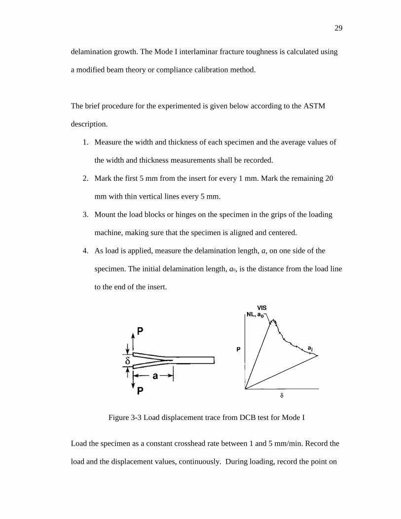
Figure 3-3 Load displacement trace from DCB test for Mode I ....................................... 29

Figure 3-4 Load v/s cross-head displacement for the four specimens .............................. 31

Figure 3-5 Modeling ASDM 5528 on Abaqus CAE ........................................................ 31

x

x

Figure ............................................................................................................................. Page

Figure 3-6 Coupled surfaces to simulate Loading Pins .................................................... 33

Figure 3-7 Boundary Conditions applied to reference points ........................................... 33

Figure 3-8 Mid plane interactions on the DCB ................................................................. 34

Figure 3-9 Initially bonded and unbonded region............................................................. 34

Figure 3-10 Delamination from VCCT interaction .......................................................... 36

Figure 3-11 Delamination from VCCT interaction .......................................................... 37

Figure 3-12 Load-Displacement graph of the DCB mode 1 ............................................. 37

Figure 3-13 Standard test specimen for EN6034 .............................................................. 39

Figure 3-14 Test fixture .................................................................................................... 39

Figure 3-15 The laod-displacement graph provided by Cytec .......................................... 41

Figure 3-16 Abaqus CAE model for EN 6034.................................................................. 42

Figure 3-17 Support and Loading Pins modeled as rigid bodies ...................................... 44

Figure 3-18 Mid-plane interaction mode II ...................................................................... 45

Figure 3-19 Initial delamination mode II .......................................................................... 45

Figure 3-20 Final mode II deformation VCCT ................................................................. 46

Figure 3-21 Final mode II deformation VCCT ................................................................. 47

Figure 3-22 Load – Displacement graph for mode II delamination ................................. 48

Figure 4-1 I-Beam- Flange, Web and Filler ...................................................................... 49

Figure 4-2 The Four-Point bend test apparatus of the I-beam .......................................... 50

Figure 4-3 Fine Mesh Region of the I-Beam .................................................................... 51

Figure 4-4 The fine mesh zone (a) with exploded view (b) .............................................. 51

Figure 4-5 Fine Mesh Zone through-thickness skin modeling approach ......................... 52

xi

xi

Figure ............................................................................................................................. Page

Figure 4-6 Truncated filler geometry ................................................................................ 53

Figure 4-7 Fine mesh zone of the filler length .................................................................. 54

Figure 4-8 Support Pins modeled as rigid bodies ............................................................. 56

Figure 4-9 Boundary conditions on the support pins ........................................................ 57

Figure 4-10 Interactions between support pins and I-Beam ............................................. 58

Figure 4-11 Interactions between top flange and filler ..................................................... 58

Figure 4-12 Bonded region of the I-Beam ........................................................................ 59

Figure 4-13 Bonded region in the Fine Mesh Zone: Filler ............................................... 59

Figure 4-14 Stresses acting on deformed body: VCCT .................................................... 60

Figure 4-15 Reaction force v/s Displacement for (a) Loading pin 1 (b) Loading Pin 2 ... 61

Figure 4-16 Stress distribution in fine mesh zone: VCCT ................................................ 62

Figure 4-17 The EFENRRTR distribution over the filler ................................................. 62

Figure 4-18 Six nodes on the crack front .......................................................................... 63

Figure 4-19 EFENNRTR v/s displacement for the six selected nodes ............................. 64

Figure 4-20 Stresses acting on final deformed model: CZM ............................................ 65

Figure 4-21 Reaction Force v/s Displacement for Loading Pins: CZM ........................... 65

Figure 4-22 CSDMG v/s Vertical Displacement for selected nodes: CZM ..................... 66

Figure 4-23 Reaction force – displacement curves for CZM and VCCT model .............. 68

xii

xii

ABSTRACT

Ramakrishna, Greeshma. M.S., Purdue University, May 2015. Delamination of C/PEKK

I-Beam Using Virtual Crack Closure Technique and Cohesive Zone Method. Major

Professor: Vikas Tomar.

In collaboration with Fokker Aerostructures B.V, a damage study is conducted on a

carbon epoxy/PEKK (poly-ether-ketone-ketone) thermoplastic composite I-Beam, with a

pre crack of 100 mm modeled between the top flange and the filler (butt joint between

filler and web). The C/PEKK I-Beam is modeled after a section of the Gulfstream G650

aircraft's center beam, which was previously a carbon fiber/epoxy hat-stiffened skin

construction. The objective of the thesis is to identify if the crack propagates in the I-

Beam within the load range that act on the current center beam of the G650 aircraft. Two

finite element methods are identified to study the crack propagation in the model, namely

virtual crack closure technique (VCCT) and the cohesive zone model (CZM). These two

methods are verified by reproducing experimental data for calculating fracture toughness

(mode I and mode II) of PEKK thermoplastic produced by CYTEC Inc., using ABAQUS

CAE. Next, the I-Beam is modeled under a four point bending load, and analysis is

performed using both the methods to study the loads at which the model begins to

delaminate. Both the approaches produce similar data, verifying the results obtained. The

model does delaminate within the range of the loads applied on the center beam.

1

CHAPTER 1. INTRODUCTION

1.1 Background

The goal of the aerospace industry is to satisfy customer requirements by enhancing

aircraft performance and minimizing acquisition and operating costs. Achieving this

goal is reliant in part on the development of ‘superior’ structural materials. Over the

past 70 years, aluminum has been the dominant aerospace structural material.

Polymer matrix composites, on the other hand, were not used in large amounts until

the1990s. The use of composites in aerospace applications has increased greatly in

the past decade. In 1982, 8% of the airbus A130 consisted of composites. Twenty

years later, the use of composites in Airbus A380 rose to 25%. In the current

generation of aircrafts, Boeing flew the 787 Dreamliner in 2009, which was made of

50% composites, and in June 2013 Airbus flew its Airbus A350 XWB which is made

up of 53% composites. Composites are conquering traditional metal domains

throughout the aircraft. In the military sector, about 35% of the structural weight of

the Airbus A-400M is composite material. As other examples, composites account for

about 25% and 35% of the Lockheed Martin F-22 Raptor and F-35 Lighting II,

respectively. Figure 1.1 shows the rapid increase in the composition of material in

the airframe with time.

2

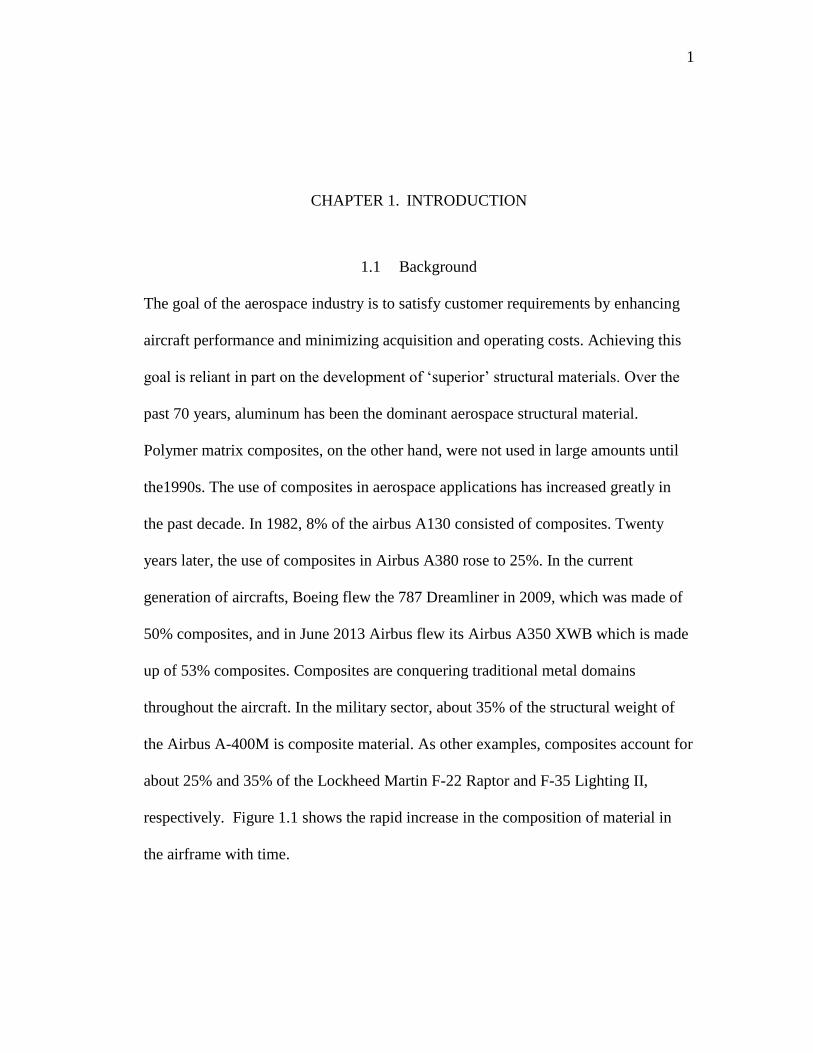
Figure 1-1 Change in Composite Manufacture Processes vs. Airframe content.

The large increase in the use of composites in aerospace applications is because they

provide important benefits over aluminum alloys, including lighter weight which

results in more fuel efficient and environmental friendly aircraft (less NOx and

greenhouse gas emissions from fuel burn) thus increasing aircraft range, payload or

maneuverability; form into more complex shapes/design; offer the capability to be

stacked/designed in such a way that the properties of the composite is tailored to best

withstand loads; fewer number of components, fasteners and joints; higher specific

3

strength, specific stiffness and fatigue resistance; excellent chemical and corrosion

resistance; and good acoustic insulation and vibration damping properties.

Today, vast majority of composite materials for aerospace are based on thermoset

materials, especially in the United States. Thermoset composites have a successful

track record dating back to 1960s, making the database very reliable. However, the

second half of the 1980s saw the emergence of a new family of composite materials,

continuous fiber reinforced thermoplastics and for the past two decades, they have

significantly matured. These composites have several key advantages over

thermosets. Since thermoset composite processes and materials are mature, cost and

weight reduction associated with design optimizations are less likely to continue.

However, since the research with regards to thermoplastics is still ongoing, it is easy

to mold it to the needs of the evolving aerospace requirements.

These thermoplastic composites are comparable to thermoset composites in the sense

that they have the same fiber reinforcements as carbon, aramid or glass fiber fabrics

or unidirectional tapes. However, a lot of justifications can be made for using higher-

cost thermoplastic composites instead of thermoset composites in aerospace

applications. Unlike thermosets, thermoplastics polymers shape easily under

sufficient heat and simply harden and maintain those shapes when cooled. They also

retain their plasticity — that is, they will remelt and can be reshaped by reheating

them above their processing temperatures. This characteristic offers intriguing

4

possibilities for both faster and more innovative composite processing techniques

compared to their thermoset counterparts.

Thus, as a result of this paradigm shift toward process/cost efficiency, reinforced

thermoplastics now appear on the cusp of capturing a significant piece of the

aerospace raw materials market as seen in Fig 1.1.

1.2 Thermoplastic Composites: What and Why

There is a wide range of thermoplastic materials now used in advanced composites

components for the aerospace industry.[1] Six general classes of thermoplastics are

seen most frequently

Poly-carbonates (PC)

Poly-amides (nylon, PA-6, PA-12)

Poly-phenylene +Sulfide (PPS)[2]

Poly-ether-imide (PEI)[3]

Poly-ether-ether-ketone (PEEK)[4]

Poly-ether-ketone-ketone (PEKK)[5]

Continuous fibre reinforced thermoplastics have a number of advantages over other

materials, a few mentioned in the previous section. Among these are improved

toughness, excellent fire resistance and recyclability. However, the primary reason for

the use of thermoplastics is cost effective processing. [6][7] Fig 1.2 shows a graph of

neat resin performance characteristics vs. raw material costs, which makes the

5

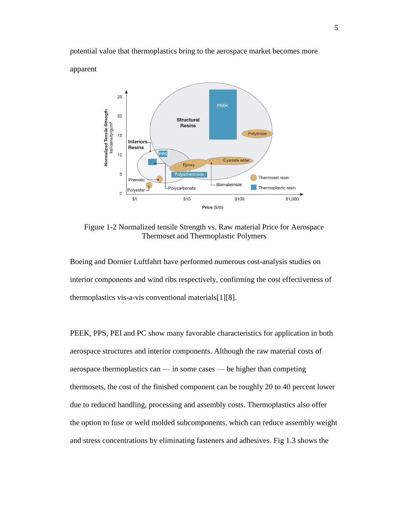
potential value that thermoplastics bring to the aerospace market becomes more

apparent

Figure 1-2 Normalized tensile Strength vs. Raw material Price for Aerospace

Thermoset and Thermoplastic Polymers

Boeing and Dornier Luftfahrt have performed numerous cost-analysis studies on

interior components and wind ribs respectively, confirming the cost effectiveness of

thermoplastics vis-a-vis conventional materials[1][8].

PEEK, PPS, PEI and PC show many favorable characteristics for application in both

aerospace structures and interior components. Although the raw material costs of

aerospace thermoplastics can — in some cases — be higher than competing

thermosets, the cost of the finished component can be roughly 20 to 40 percent lower

due to reduced handling, processing and assembly costs. Thermoplastics also offer

the option to fuse or weld molded subcomponents, which can reduce assembly weight

and stress concentrations by eliminating fasteners and adhesives. Fig 1.3 shows the

6

timeline of the use of thermoplastic composites in commercial aircrafts, as per Fokker

Aerostructures B.V.

Figure 1-3 Thermoplastic Composites in Commercial Aircraft:

Now let us discuss the types of thermoplastics available and how they can be used as

aircraft primary structures. With regard to high performance applications the early

thermoplastics were insufficiently resistant to heat and moisture. The first high

performance composites to become available had PEEK [4](Poly-Ether-Ether-

Ketone) as a matrix. After this first step the need grew for a more affordable material

that was easier to handle in production. PEI (Poly-Ether-Imide) [3]was next to be

applied in structural parts. It was quite successful but it did have a drawback: it was

sensitive to the kind of aggressive fluids that live in wide body aircraft. A better

polymer had to be developed. With the year 2000 approaching this became PPS

(Poly- Phenylene-Sulfide). No material is perfect for every application. PPS is widely

7

used, but its surface energy and shrinkage behaviour leave room for PEKK (Poly-

Ether-Ketone-Ketone)[5]. Currently the most commonly used is the latest version of

PPS, but the choice between PEEK, PEKK, PEI and PPS is fine-tuned to functional

and process requirements. Affordability and weight are the determinant factors.

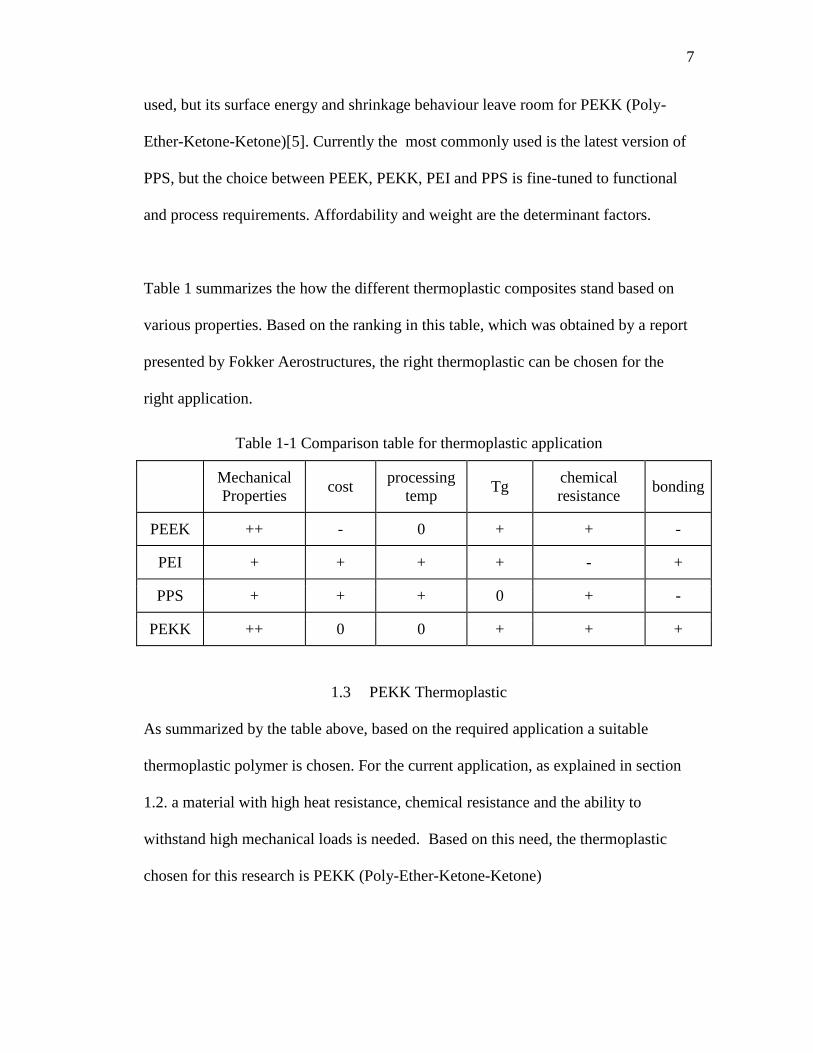
Table 1 summarizes the how the different thermoplastic composites stand based on

various properties. Based on the ranking in this table, which was obtained by a report

presented by Fokker Aerostructures, the right thermoplastic can be chosen for the

right application.

Table 1-1 Comparison table for thermoplastic application

Mechanical

Properties cost

processing

temp Tg

chemical

resistance bonding

PEEK ++ - 0 + + -

PEI + + + + - +

PPS + + + 0 + -

PEKK ++ 0 0 + + +

1.3 PEKK Thermoplastic

As summarized by the table above, based on the required application a suitable

thermoplastic polymer is chosen. For the current application, as explained in section

1.2. a material with high heat resistance, chemical resistance and the ability to

withstand high mechanical loads is needed. Based on this need, the thermoplastic

chosen for this research is PEKK (Poly-Ether-Ketone-Ketone)

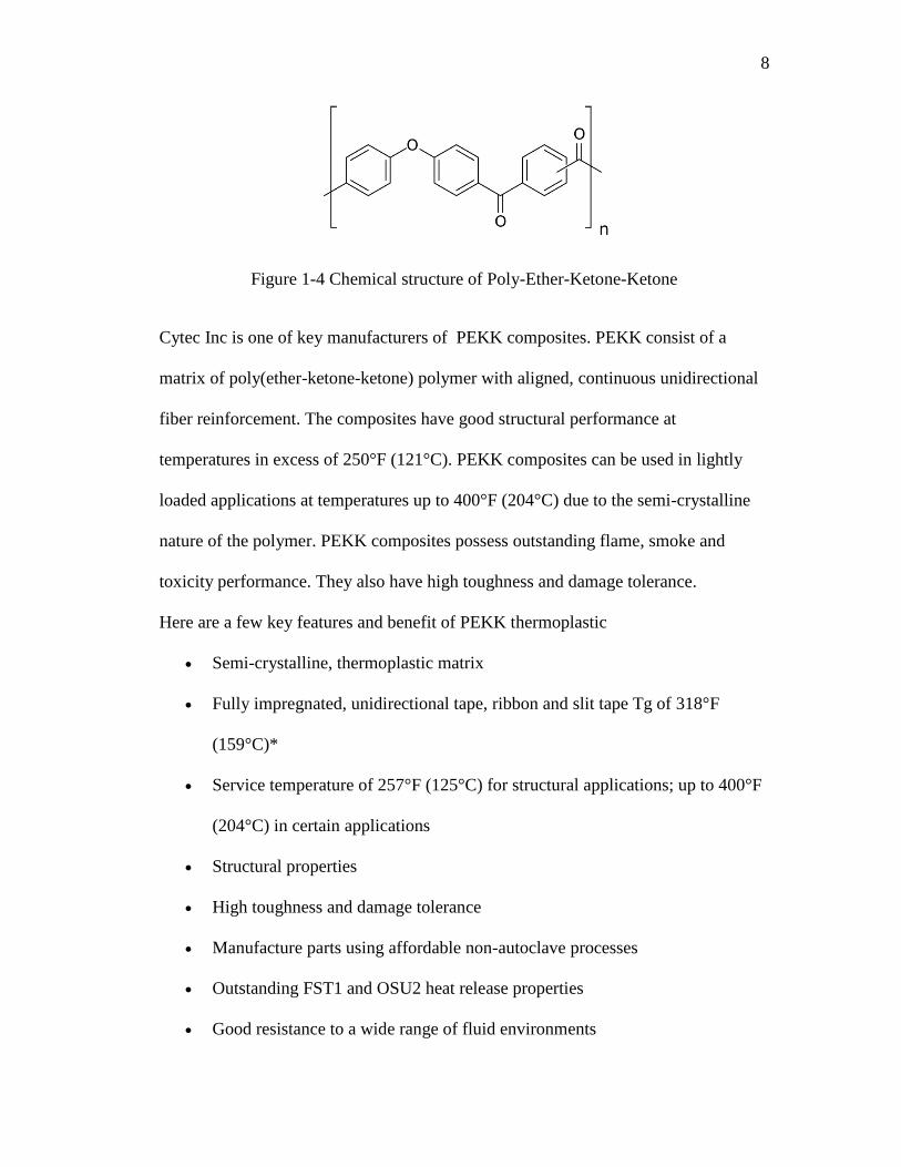
8

Figure 1-4 Chemical structure of Poly-Ether-Ketone-Ketone

Cytec Inc is one of key manufacturers of PEKK composites. PEKK consist of a

matrix of poly(ether-ketone-ketone) polymer with aligned, continuous unidirectional

fiber reinforcement. The composites have good structural performance at

temperatures in excess of 250°F (121°C). PEKK composites can be used in lightly

loaded applications at temperatures up to 400°F (204°C) due to the semi-crystalline

nature of the polymer. PEKK composites possess outstanding flame, smoke and

toxicity performance. They also have high toughness and damage tolerance.

Here are a few key features and benefit of PEKK thermoplastic

Semi-crystalline, thermoplastic matrix

Fully impregnated, unidirectional tape, ribbon and slit tape Tg of 318°F

(159°C)*

Service temperature of 257°F (125°C) for structural applications; up to 400°F

(204°C) in certain applications

Structural properties

High toughness and damage tolerance

Manufacture parts using affordable non-autoclave processes

Outstanding FST1 and OSU2 heat release properties

Good resistance to a wide range of fluid environments

9

Low moisture uptake, < 0.3 wt%3

Indefinite shelf life at room temperature

Recyclable

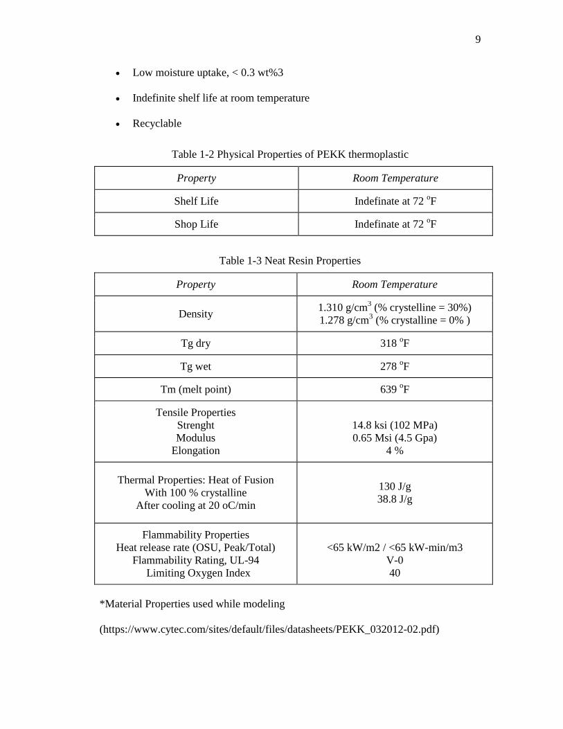
Table 1-2 Physical Properties of PEKK thermoplastic

Property Room Temperature

Shelf Life Indefinate at 72 oF

Shop Life Indefinate at 72 oF

Table 1-3 Neat Resin Properties

Property Room Temperature

Density 1.310 g/cm

3 (% crystelline = 30%)

1.278 g/cm3 (% crystalline = 0% )

Tg dry 318 oF

Tg wet 278 oF

Tm (melt point) 639 oF

Tensile Properties

Strenght

Modulus

Elongation

14.8 ksi (102 MPa)

0.65 Msi (4.5 Gpa)

4 %

Thermal Properties: Heat of Fusion

With 100 % crystalline

After cooling at 20 oC/min

130 J/g

38.8 J/g

Flammability Properties

Heat release rate (OSU, Peak/Total)

Flammability Rating, UL-94

Limiting Oxygen Index

<65 kW/m2 / <65 kW-min/m3

V-0

40

*Material Properties used while modeling

(https://www.cytec.com/sites/default/files/datasheets/PEKK_032012-02.pdf)

10

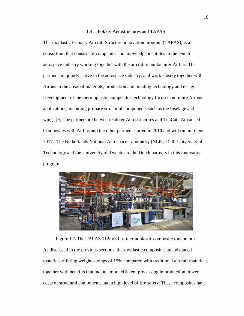
1.4 Fokker Aerostructures and TAPAS

Thermoplastic Primary Aircraft Structure innovation program (TAPAS), is a

consortium that consists of companies and knowledge institutes in the Dutch

aerospace industry working together with the aircraft manufacturer Airbus. The

partners are jointly active in the aerospace industry, and work closely together with

Airbus in the areas of materials, production and bonding technology and design.

Development of the thermoplastic composites technology focuses on future Airbus

applications, including primary structural components such as the fuselage and

wings.[9] The partnership between Fokker Aerostructures and TenCate Advanced

Composites with Airbus and the other partners started in 2010 and will run until end-

2017. The Netherlands National Aerospace Laboratory (NLR), Delft University of

Technology and the University of Twente are the Dutch partners in this innovation

program.

Figure 1-5 The TAPAS 112m/39 ft- thermoplastic composite torsion box

As discussed in the previous sections, thermoplastic composites are advanced

materials offering weight savings of 15% compared with traditional aircraft materials,

together with benefits that include more efficient processing in production, lower

costs of structural components and a high level of fire safety. These composites have

11

high strength, light weight and contribute to the drive towards sustainable aviation,

because the use of these materials allows constant reductions in aircraft weight to be

achieved. As a result fuel consumption is reduced, the range of the aircraft is

increased and higher payloads are possible. The target is to further increase the

proportion of thermoplastic composites in current aircraft as well as in the new

generation of aircraft. A thermoplastic fuselage panel has been produced and

presented as demonstrator as part of TAPAS 1. Currently, a demonstration tail section

made entirely of thermoplastic composite material is being developed under the

TAPAS 2 agreement. In the long term, the hope is to prove Thermoplastics as a

viable option as a successor to a narrow body program.

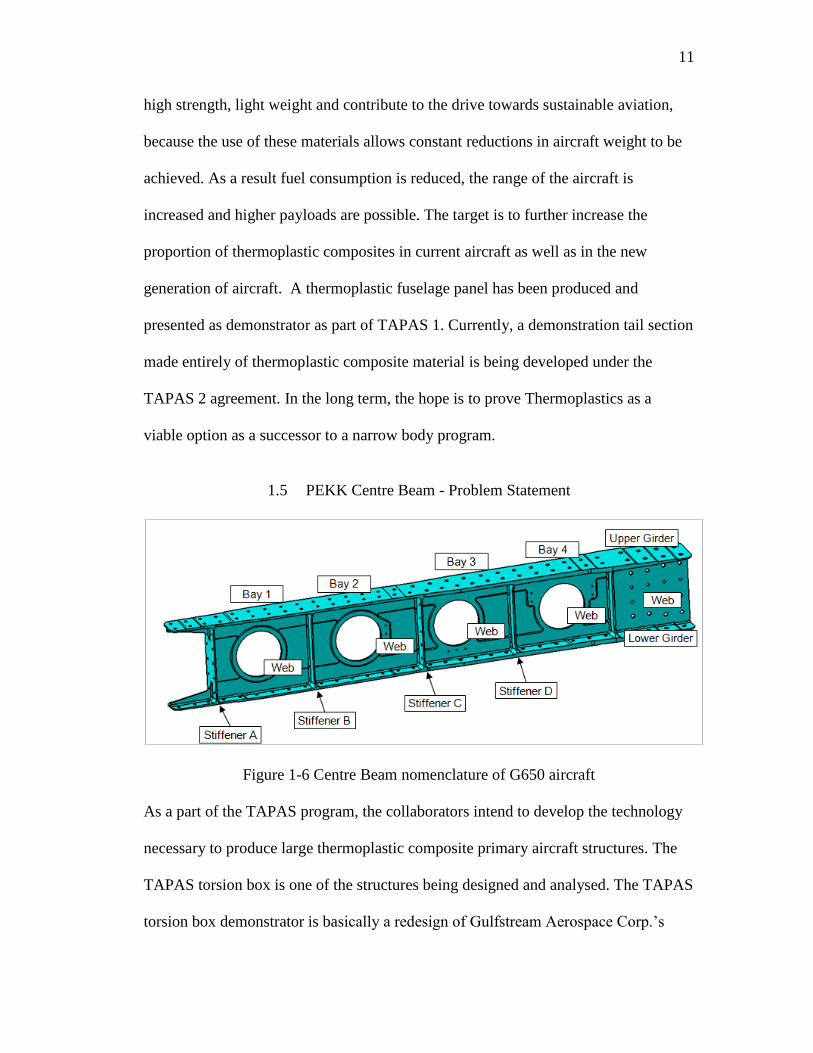
1.5 PEKK Centre Beam - Problem Statement

Figure 1-6 Centre Beam nomenclature of G650 aircraft

As a part of the TAPAS program, the collaborators intend to develop the technology

necessary to produce large thermoplastic composite primary aircraft structures. The

TAPAS torsion box is one of the structures being designed and analysed. The TAPAS

torsion box demonstrator is basically a redesign of Gulfstream Aerospace Corp.’s

12

(Savannah, Ga.) Gulfstream G650 horizontal stabilizer, previously a carbon

fiber/epoxy hat-stiffened skin construction. The torsion box is the fixed structure of

the tail, and it is more heavily loaded than the movable rudder and elevators, which

Fokker now produces in carbon/PPS, achieving a 10 percent weight reduction and a

20 percent cost savings vs. previous carbon/epoxy. The torsion box features tailored

skins with varying thickness, from 2 mm/0.08 inch at its thinnest to 8 mm/0.4 inch at

the root, and will be made from unidirectional carbon fiber/PEKK.

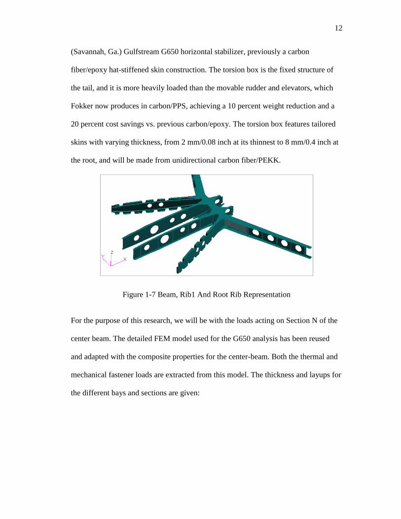
Figure 1-7 Beam, Rib1 And Root Rib Representation

For the purpose of this research, we will be with the loads acting on Section N of the

center beam. The detailed FEM model used for the G650 analysis has been reused

and adapted with the composite properties for the center-beam. Both the thermal and

mechanical fastener loads are extracted from this model. The thickness and layups for

the different bays and sections are given:

13

Figure 1-8 Centre beam section classification

Table 1-4 Geometry for Section N

Part Parameter Dimension (mm)

Flange

Plies 58

Width 80

Thickness 8.004

Web

Plies 40

Width 175.4

Thickness 5.52

G650 TAPAS G650 TAPAS G650 TAPAS G650 TAPAS

Upper Flange t [mm] 4.80 4.97 5.55 6.07 7.10 8.00 9.81 10.21 9.70 7.50 5.00 2.70 8.00 6.62 4.97 4.97

Web t [mm] 2.35 4.28 2.78 4.28 5.45 5.52 5.35 5.52

Lower Flange t [mm] 3.75 4.97 4.64 6.07 6.67 8.00 9.21 10.21 7.70 5.50 4.00 3.00 8.00 6.62 4.97 4.97

Stiffener A [mm] 2.70 1.66

Stiffener B [mm] 2.70 2.07

Stiffener C [mm] 2.80 2.07

Stiffener D [mm] 3.40 2.21

Stiffener E [mm]

G650 TAPAS G650 TAPAS G650 TAPAS G650 TAPAS

Upper Flange t [# plies] 36 44 58 74 58 48 36 36

Web t [# plies] 31 31 40 40

Lower Flange t [# plies] 36 44 58 74 58 48 36 36

Stiffener A [# plies] 12

Stiffener B [# plies] 15

Stiffener C [# plies] 15

Stiffener D [# plies] 16

Stiffener E [# plies]

TAPAS

2.48

TAPAS

Joints PF

5.52

Joints PF

Bay 1 Bay 2 Bay 3 Bay 4

Bay 1 Bay 2 Bay 3 Bay 4

40

G650

3.50

4.00

18

A B C D E

14

According to data reported by Fokker Aerostructures, the load acting on the web,

section N is 273 N/mm.

1.5.1 Objective of Project

There is a two-step objective for this Masters’ research

1. Model the loading apparatus and the center beam in PEKK thermoplastic

with a preexisting crack.

2. To apply the loads that is extracted from the G650 analysis and study the

delamination, if any.

1.5.2 Scope of Project

The center beam is modeled as a uniform cross section I-beam, with the dimensions

of the Rib3, Section N, using the composite layup provided in the previous section. A

filler material is included between the flange and web as requested by Fokker

Aerostructures. The loads are simulated by placing the I-beam under a four point

bend experiment.

To analyze the delamination ABAQUS CAE is used, implementing two finite

element methods: Virtual Crack Closure Technique (VCCT) and Cohesive Zone

Method (CZM). The two methods are first validated by reproducing experimental

data for calculating fracture toughness for PEKK Thermoplastic conducted by

CYTEC Inc., for pure mode I and mode II delamination.

15

Finally, the C/PEKK I-beam is modeled in ABAQUS CAE, with an initial crack

between the upper flange and filler. Under the four point bend test, the composite

beam is subjected to mode II (or sliding mode) delamination. The delamination is

analyzed using both virtual crack closure technique (VCCT) and cohesive zone

method (CZM), to observe if there is crack propagation within the loads applied.

Figure 1-9 Scope of the Project

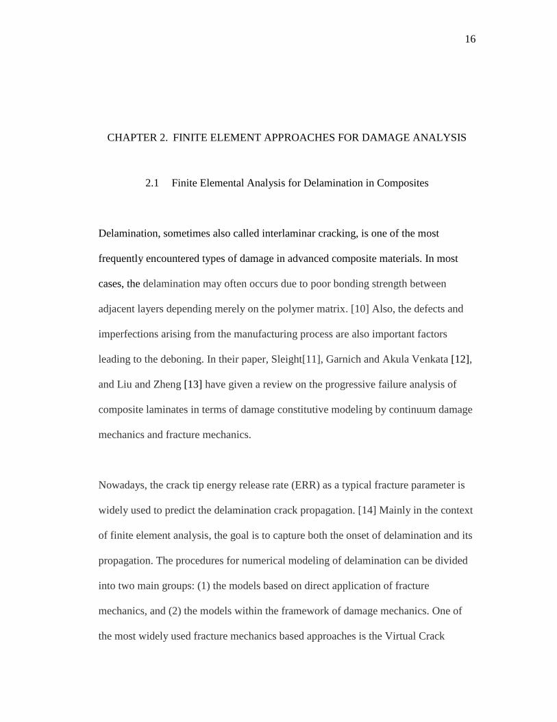
16

CHAPTER 2. FINITE ELEMENT APPROACHES FOR DAMAGE ANALYSIS

2.1 Finite Elemental Analysis for Delamination in Composites

Delamination, sometimes also called interlaminar cracking, is one of the most

frequently encountered types of damage in advanced composite materials. In most

cases, the delamination may often occurs due to poor bonding strength between

adjacent layers depending merely on the polymer matrix. [10] Also, the defects and

imperfections arising from the manufacturing process are also important factors

leading to the deboning. In their paper, Sleight[11], Garnich and Akula Venkata [12],

and Liu and Zheng [13] have given a review on the progressive failure analysis of

composite laminates in terms of damage constitutive modeling by continuum damage

mechanics and fracture mechanics.

Nowadays, the crack tip energy release rate (ERR) as a typical fracture parameter is

widely used to predict the delamination crack propagation. [14] Mainly in the context

of finite element analysis, the goal is to capture both the onset of delamination and its

propagation. The procedures for numerical modeling of delamination can be divided

into two main groups: (1) the models based on direct application of fracture

mechanics, and (2) the models within the framework of damage mechanics. One of

the most widely used fracture mechanics based approaches is the Virtual Crack

17

Closure Technique [15][16] (VCCT). This approach is based on Linear Elastic

Fracture Mechanics (LEFM) and requires an initial crack to predict the delamination.

Another widely used approach for modeling delamination based on damage

mechanics is the cohesive elements based on the cohesive zone models [17][18]. A

cohesive damage zone is assumed at the crack tip, and the model relates tractions to

displacement jumps at an interface where a crack may take place. Both of these state-

of-the-art methods have been incorporated into the ABAQUS® finite element

software [19] for the simulation of initiation and extension of delamination.

2.2 Virtual Crack Closure Technique (VCCT)

2.2.1 Introduction

Delamination is the most commonly studied modes of failure in composites. Thus,

fracture mechanics principles (Janssen et al., 2004) can be used to study the behavior

of composite structures in presence of interlaminar damage and to identify the

conditions when the forces start to propagate. Making the assumption that growth of

delamination is the same as crack propagation[20][21], the science and mathematics

of fracture mechanics can be used to study delamination as well. The propagation of a

crack is possible when the energy released for unit width and length of fracture

surface (named Strain Energy Release Rate, G) is equal to threshold level or fracture

toughness, a physical characteristic for each material. Starting from the earlier

analytical works by Chai et al.[22], and Kardomates[23][24] , delamination in

composites has been studied by calculating the Strain Energy Release Rate at the

18

crack tip. Nowadays, the G calculation is generally performed by using finite element

methods, such as the Virtual Crack Closure Technique.

From the definition mentioned above, the Energy Release Rate can be written as in

Eq.(1).

G = lim 𝛥𝑎 → 0 𝑊

𝛥𝑎 (1)

According to the Virtual Crack Closure Technique, the Strain Energy Release Rate is

calculated based on the assumption that for an infinitesimal crack opening, the strain

energy released is equal to the amount of the work required to close the crack.

Inititally, the work W required to close the crack can be evaluated by performing two

analyses. The first analysis is needed to evaluate the stress field at the crack tip for a

crack of length a and the second one is aimed to obtain displacements in the

configuration with the crack front appropriately extended from a to a+Δa. However,

today the method has been simplified to one step, by making a simple additional

assumption: an infinitesimal crack extension has negligible effects on the crack front

therefore both stress and displacement can be evaluated within the same configuration

by performing only one analysis.

Thus, by adopting this technique, the expression of the work W required to close the

crack becomes as in Eq. (2).

𝑊 = 1

2[∫ σ𝑦𝑦

(𝑎)(𝑥)Δa

0δ𝑢𝑦

(𝑎)(𝑥 − Δa)𝑑𝑥 + ∫ σ𝑦𝑥(𝑎)(𝑥)

Δa

0δ𝑢𝑥

(𝑎)(𝑥 − Δa)𝑑𝑥 + ∫ σ𝑦𝑧(𝑎)(𝑥)

Δa

0δ𝑢𝑧

(𝑎)(𝑥 −

Δa)𝑑𝑥] (2)

19

where both displacements and stress are evaluated in the same configuration.

Now, combining the equation for the Energy Release Rate and the governing

equation for One step- VCCT, (equations 1 and 2) it is possible to obtain the

expression of the Strain Energy Release Rate for the three mutually orthogonal

fracture modes: GI , GII and GIII that correspond to opening mode I, in-plane shear

mode II and antiplanar shear mode III respectively.

2.2.2 Finite Element Implementation

As mentioned above, the state of delamination in a composite structure is determined

by the comparing the Strain Energy Release Rate (G) with the fracture toughness (Gc)

of the material, for a particular mode. We see a delamination only when the G

numerically exceeds Gc . (Eq. 3)

G > Gc (3)

However, for three orthogonal modes of loading, we have respective fracture modes

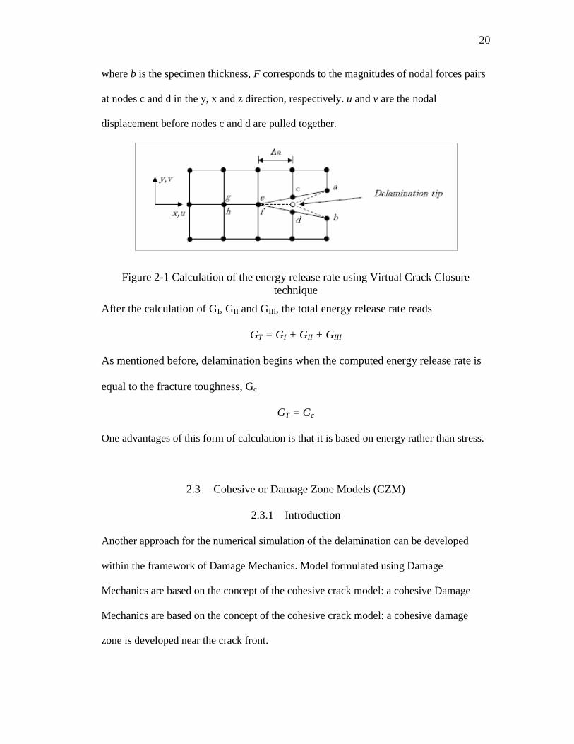
defined. In a finite element model such as shown in Figure below, the energy released is

the work done by the nodal forces required to close the crack tip, therefore:

𝐺𝐼 = 1

2𝑏Δa𝐹𝑐𝑑

𝑦(𝑣𝑐 − 𝑣𝑑)

𝐺𝐼𝐼 = 1


𝑥 (𝑢𝑐 − 𝑢𝑑)

𝐺𝐼𝐼𝐼 = 1


𝑦𝑧(𝑤𝑐 − 𝑤𝑑) (4)

20

where b is the specimen thickness, F corresponds to the magnitudes of nodal forces pairs

at nodes c and d in the y, x and z direction, respectively. u and v are the nodal

displacement before nodes c and d are pulled together.

Figure 2-1 Calculation of the energy release rate using Virtual Crack Closure

technique

After the calculation of GI, GII and GIII, the total energy release rate reads

GT = GI + GII + GIII

As mentioned before, delamination begins when the computed energy release rate is

equal to the fracture toughness, Gc

GT = Gc

One advantages of this form of calculation is that it is based on energy rather than stress.

2.3 Cohesive or Damage Zone Models (CZM)

2.3.1 Introduction

Another approach for the numerical simulation of the delamination can be developed

within the framework of Damage Mechanics. Model formulated using Damage

Mechanics are based on the concept of the cohesive crack model: a cohesive Damage

Mechanics are based on the concept of the cohesive crack model: a cohesive damage

zone is developed near the crack front.

21

Cohesive damage zone models relate traction forces in the defined cohesive zone to

displacement discontinuities at the crack tip. Damage initiation depends on the maximum

value of the traction forces, in the traction-displacement curve (T-∆). When the area

under the traction-displacement graph is equal to the fracture toughness Gc, the traction is

reduced to zero and new crack surfaces are formed.

The advantages of the CZM approach are its unification of crack initiation and

growth into one model. Cohesive zone model formulations are more powerful than

fracture mechanics because they allow the prediction of both initiation and crack

propagation. The formulation and finite element implementation is described below.

In the simplest and most usual formulation of CZM, the entire body under

consideration is assumed to be linear elastic, while the area in the cohesive zone is

embedded with the non-linear cohesive law (Fig. 2.3). The cohesive law dictates the

interfacial law that acts on the crack line. The stress in the cohesive law is the

cohesive strength of the material, σc, while the area under the curve is the cohesive

fracture energy, Gc. The entire fracture process can be summarized in Fig. 1: In stage

1, the linear elastic behavior of the model, as mentioned in the assumption, prevails.

As the load increases at the crack front, the crack initiates (2). The region with 2 and

3 is the area governed by the cohesive law, which in nonlinear and grows from

initiation to full failure. At 4, when the area under the area under the curve equals the

fracture toughens, a new traction free surface appears (∆=∆c).

22

Figure 2-2 Cohesive zone modeling of fracture

Figure 2-3 Cohesive Law

Therefore, the continuum should be characterized by two constitutive laws; for

instance, a linear stress-strain relation for the bulk material and a cohesive surface

relation (cohesive law) that allows crack spontaneous initiation and growth.

23

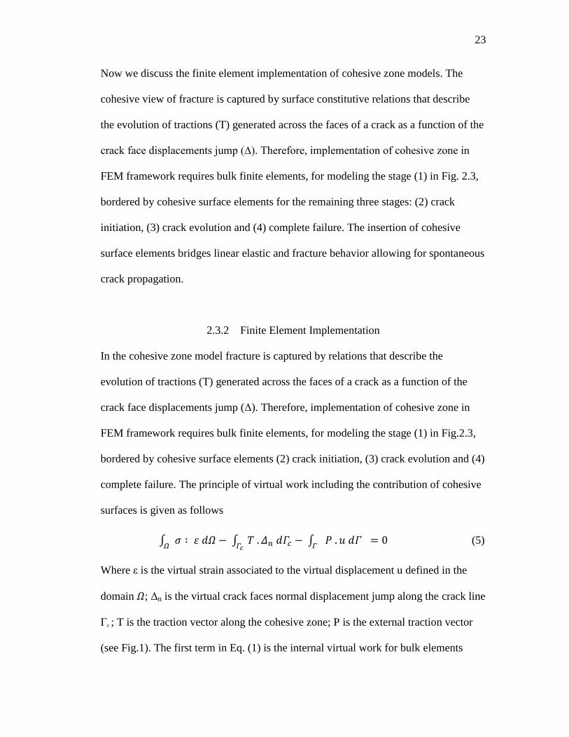
Now we discuss the finite element implementation of cohesive zone models. The

cohesive view of fracture is captured by surface constitutive relations that describe

the evolution of tractions (T) generated across the faces of a crack as a function of the

crack face displacements jump (∆). Therefore, implementation of cohesive zone in

FEM framework requires bulk finite elements, for modeling the stage (1) in Fig. 2.3,

bordered by cohesive surface elements for the remaining three stages: (2) crack

initiation, (3) crack evolution and (4) complete failure. The insertion of cohesive

surface elements bridges linear elastic and fracture behavior allowing for spontaneous

crack propagation.

2.3.2 Finite Element Implementation

In the cohesive zone model fracture is captured by relations that describe the

evolution of tractions (T) generated across the faces of a crack as a function of the

crack face displacements jump (Δ). Therefore, implementation of cohesive zone in

FEM framework requires bulk finite elements, for modeling the stage (1) in Fig.2.3,

bordered by cohesive surface elements (2) crack initiation, (3) crack evolution and (4)

complete failure. The principle of virtual work including the contribution of cohesive

surfaces is given as follows

∫ 𝜎 ∶ 𝜀 𝑑𝛺𝛺

− ∫ 𝑇 . 𝛥𝑛 𝑑𝛤𝑐𝛤𝑐− ∫ 𝑃 . 𝑢 𝑑𝛤

𝛤= 0 (5)

Where ε is the virtual strain associated to the virtual displacement u defined in the

domain 𝛺; Δn is the virtual crack faces normal displacement jump along the crack line

Γc ; T is the traction vector along the cohesive zone; P is the external traction vector

(see Fig.1). The first term in Eq. (1) is the internal virtual work for bulk elements

24

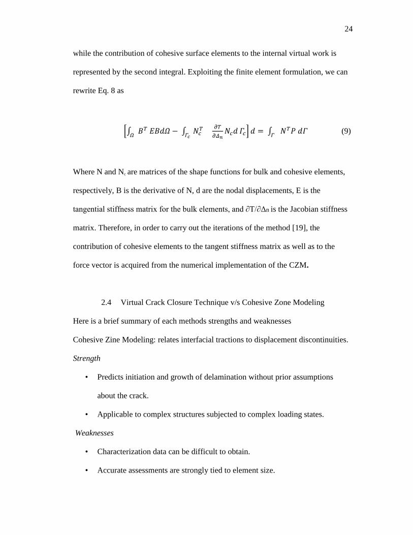
while the contribution of cohesive surface elements to the internal virtual work is

represented by the second integral. Exploiting the finite element formulation, we can

rewrite Eq. 8 as

[∫ 𝐵𝑇 𝐸𝐵𝑑𝛺𝛺

− ∫ 𝑁𝑐𝑇

𝜕𝑇

𝜕𝛥𝑛𝑁𝑐𝑑

𝛤𝑐𝛤𝑐] 𝑑 = ∫ 𝑁𝑇𝑃 𝑑𝛤

𝛤 (9)

Where N and Nc are matrices of the shape functions for bulk and cohesive elements,

respectively, B is the derivative of N, d are the nodal displacements, E is the

tangential stiffness matrix for the bulk elements, and ∂T/∂Δn is the Jacobian stiffness

matrix. Therefore, in order to carry out the iterations of the method [19], the

contribution of cohesive elements to the tangent stiffness matrix as well as to the

force vector is acquired from the numerical implementation of the CZM.

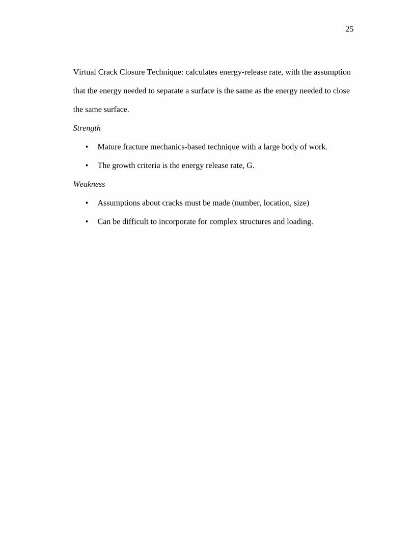
2.4 Virtual Crack Closure Technique v/s Cohesive Zone Modeling

Here is a brief summary of each methods strengths and weaknesses

Cohesive Zine Modeling: relates interfacial tractions to displacement discontinuities.

Strength

• Predicts initiation and growth of delamination without prior assumptions

about the crack.

• Applicable to complex structures subjected to complex loading states.

Weaknesses

• Characterization data can be difficult to obtain.

• Accurate assessments are strongly tied to element size.

25

Virtual Crack Closure Technique: calculates energy-release rate, with the assumption

that the energy needed to separate a surface is the same as the energy needed to close

the same surface.

Strength

• Mature fracture mechanics-based technique with a large body of work.

• The growth criteria is the energy release rate, G.

Weakness

• Assumptions about cracks must be made (number, location, size)

• Can be difficult to incorporate for complex structures and loading.

26

CHAPTER 3. VALIDATION OF FE METHODS USING ABAQUS CAE

3.1 Three modes of Crack Extension

Delamination fracture may occur in three different loadings, referred to as opening or

peel mode (mode I), forward sliding shear mode (mode II), and tearing mode (mode

III). As shown in figure 3.1 these modes are based on the loading condition and

relative displacements of the crack faces. The resistance to delamination growth is

expressed in terms of delamination fracture toughness, which is generally measured

experimentally. Numerous studies have attempted to determine delamination criterion

based on the resistance to delamination due to mixed-loadings by combination of pure

modes [29].

For this thesis research, the two methods mentioned in Chapter 2 are verified and

validated using the experimental results provided Cytec Inc. for PEKK thermoplastic

polymer. The experiments are simulated based on the ASTM standards for pure mode

I and II. The experimental data was provided to Fokker Aerostructures as part of the

TAPAS program.

27

Figure 3-1 Three modes of delamination in composite structures

3.2 MODE I Delamination

Mode 1 delamination also knows as the opening or peel mode. To determine the

Mode I interlaminar fracture toughness GIC of a fiber-reinforces composite material,

ASTM has defined a standard experimental procedure using a double cantilever

beam; ASTM D5528 ‘Standard Test Method for Mode 1 Interlaminar Fracture

Toughness of Unidirectional Fiber-Reinforced Polymer Matrix Composites’.

This test method is limited to use with composites consisting of unidirectional carbon

fiber and glass fiber tape laminates with brittle and tough single-phase polymer

matrices. The energy release rate G, which is defined as the loss of energy, dU, in the

test specimen per unit of specimen width for an infinitesimal increase in delamination

length, da, for delamination growing under a constant displacement, can be

mathematically represented as

𝐺 = − 1

𝑏

𝑑𝑈

𝑑𝑎

28

Where U is the total elastic energy in the test specimen, b is the specimen width and a

is the delamination length. Fig 3.1 describes the experimental set up for the ASTM

D5528.

Figure 3-2 Double cantilever beam specimen with loading blocks

3.2.1 Experimental Test Method and Cytec results

The DCB shown in Fig 3.1 consists of a rectangular, uniform thickness,

unidirectional laminated composite specimen containing a non adhesive insert of the

midplane that serves as a delamination initiation. Opening forces are applied to the

DCB specimen by means of the loading blocks bonded to one end of the specimen.

The ends of the DCB are opened by controlling either the opening discplacement or

the crosshead movement, while the load and delamiantion lengtha are recorded.

A record of the applied load versus opening displacement is recorded on an X-Y

recorder or equivalent real-time plotting device or stored digitally and post-processed.

Instantaneous delamination front locations are marked on the chart at intervals of

29

delamination growth. The Mode I interlaminar fracture toughness is calculated using

a modified beam theory or compliance calibration method.

The brief procedure for the experimented is given below according to the ASTM

description.

1. Measure the width and thickness of each specimen and the average values of

the width and thickness measurements shall be recorded.

2. Mark the first 5 mm from the insert for every 1 mm. Mark the remaining 20

mm with thin vertical lines every 5 mm.

3. Mount the load blocks or hinges on the specimen in the grips of the loading

machine, making sure that the specimen is aligned and centered.

4. As load is applied, measure the delamination length, a, on one side of the

specimen. The initial delamination length, a0, is the distance from the load line

to the end of the insert.

Figure 3-3 Load displacement trace from DCB test for Mode I

Load the specimen as a constant crosshead rate between 1 and 5 mm/min. Record the

load and the displacement values, continuously. During loading, record the point on

30

the load-displacement curve as can be seen Fig 3.3., values at which the onset of

delamination movement from the pre-crack is observed on the edge of the specimen

(VIS, Fig 3.3).

Cytec followed the above procedures with four specimens as mentioned above. The

physical properties of the four specimens are mentioned in Table 3.1.

Table 3-1 CYTEC Inc. sample specimen

Specimen

No.

Width

(mm)

Thickness

(mm)

Cured Ply

Thickness

(mm)

No of plies Pre-Crack

length, a0

(mm)

1 25.5 4.29 0.143 30 57.0

2 25.5 4.24 0.141 30 57.7

3 25.5 4.22 0.140 30 56.7

4 25.5 4.23 0.141 30 57.3

Average 25.5 4.24 0.141 30 57.17

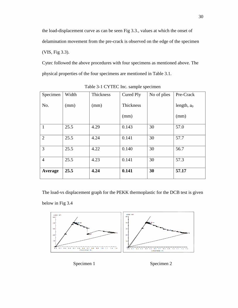
The load-vs displacement graph for the PEKK thermoplastic for the DCB test is given

below in Fig 3.4

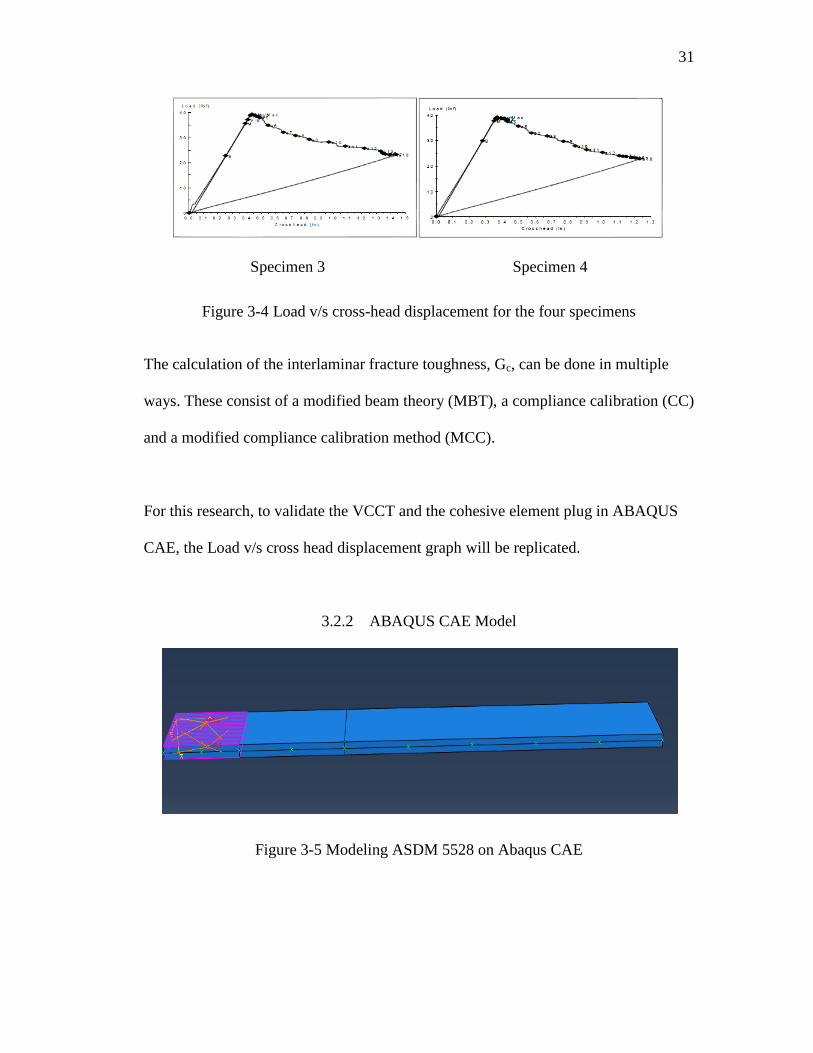
Specimen 1 Specimen 2

31

Specimen 3 Specimen 4

Figure 3-4 Load v/s cross-head displacement for the four specimens

The calculation of the interlaminar fracture toughness, Gc, can be done in multiple

ways. These consist of a modified beam theory (MBT), a compliance calibration (CC)

and a modified compliance calibration method (MCC).

For this research, to validate the VCCT and the cohesive element plug in ABAQUS

CAE, the Load v/s cross head displacement graph will be replicated.

3.2.2 ABAQUS CAE Model

Figure 3-5 Modeling ASDM 5528 on Abaqus CAE

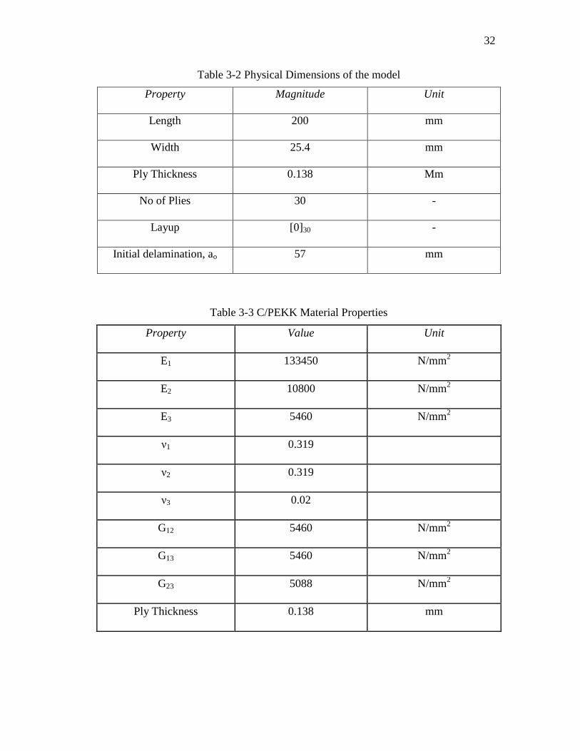
32

Table 3-2 Physical Dimensions of the model

Property Magnitude Unit

Length 200 mm

Width 25.4 mm

Ply Thickness 0.138 Mm

No of Plies 30 -

Layup [0]30 -

Initial delamination, ao 57 mm

Table 3-3 C/PEKK Material Properties

Property Value Unit

E1 133450 N/mm2

E2 10800 N/mm2

E3 5460 N/mm2

ν1 0.319

ν2 0.319

ν3 0.02

G12 5460 N/mm2

G13 5460 N/mm2

G23 5088 N/mm2

Ply Thickness 0.138 mm

33

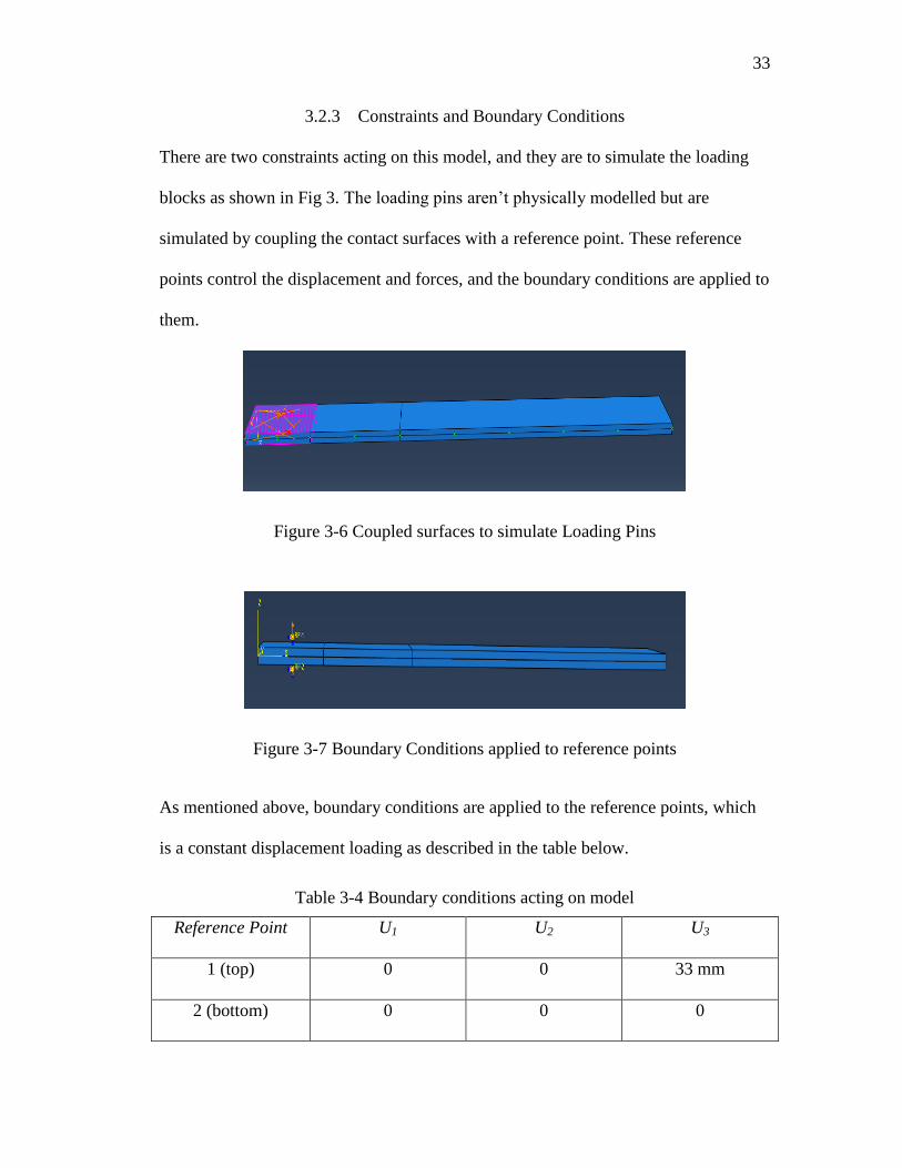
3.2.3 Constraints and Boundary Conditions

There are two constraints acting on this model, and they are to simulate the loading

blocks as shown in Fig 3. The loading pins aren’t physically modelled but are

simulated by coupling the contact surfaces with a reference point. These reference

points control the displacement and forces, and the boundary conditions are applied to

them.

Figure 3-6 Coupled surfaces to simulate Loading Pins

Figure 3-7 Boundary Conditions applied to reference points

As mentioned above, boundary conditions are applied to the reference points, which

is a constant displacement loading as described in the table below.

Table 3-4 Boundary conditions acting on model

Reference Point U1 U2 U3

1 (top) 0 0 33 mm

2 (bottom) 0 0 0

34

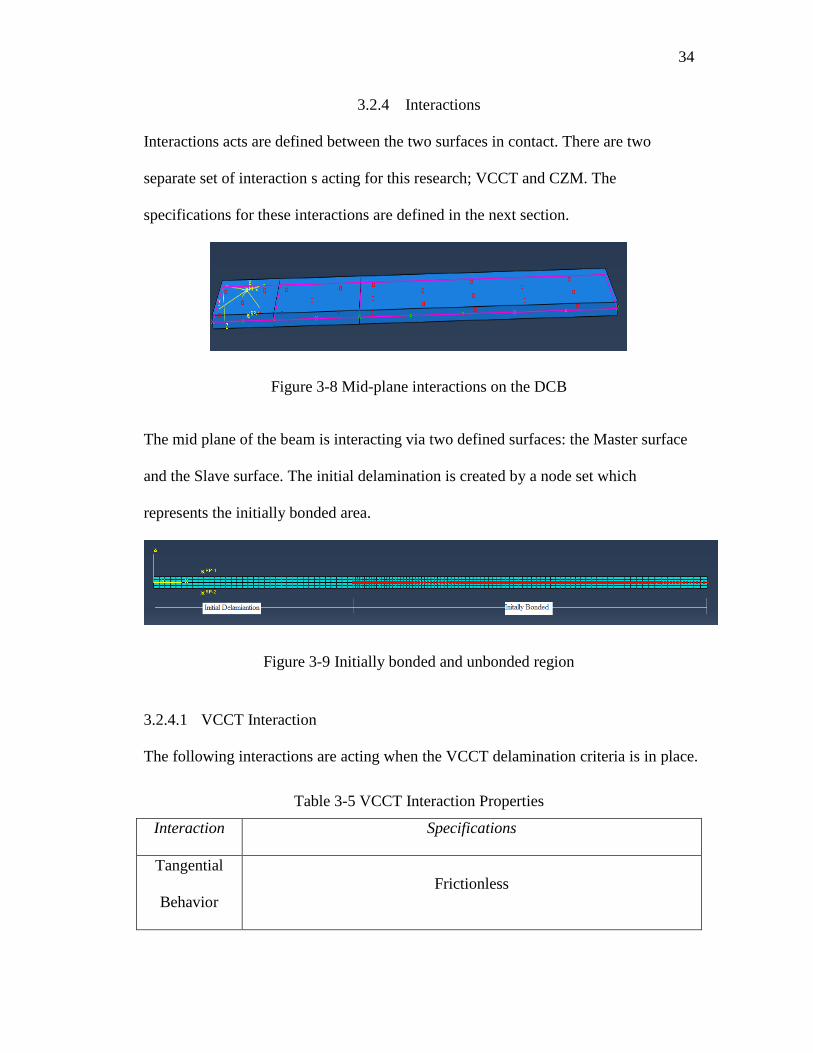
3.2.4 Interactions

Interactions acts are defined between the two surfaces in contact. There are two

separate set of interaction s acting for this research; VCCT and CZM. The

specifications for these interactions are defined in the next section.

Figure 3-8 Mid-plane interactions on the DCB

The mid plane of the beam is interacting via two defined surfaces: the Master surface

and the Slave surface. The initial delamination is created by a node set which

represents the initially bonded area.

Figure 3-9 Initially bonded and unbonded region

3.2.4.1 VCCT Interaction

The following interactions are acting when the VCCT delamination criteria is in place.

Table 3-5 VCCT Interaction Properties

Interaction Specifications

Tangential

Behavior

Frictionless

35

Normal

Behavior

Pressure Behavior = Hard contact

Fracture

Criterion:

VCCT

Critical

Energy

Release Rate

Mode I =

1.5

Mode II =

4.7

Mode III =

4.7

Exponent

= 1.75

3.2.4.2 CZM Interaction

Table 3-6 CZM Interaction Properties

Interaction Specifications

Tangential

Behavior

Frictionless

Normal

Behavior

Pressure Behavior = Hard contact

Cohesive

Behavior

Traction-

Separation

Behavior

Knn = 1e6 Kss = 1e6 Ktt = 1e6

Damage

Initiation

(Maximum

Nominal

Stresses)

Normal = 80 Shear1 = 122 Shear2 = 122

Evolution

(Linear Energy

following

Normal

Fracture

Energy = 1.35

Shear1

Fracture

Energy = 5

Shear2

Fracture

Energy = 5

36

Benzeggagh-

Kenane Law)

BK Exponent =

1.45

3.2.5 RESULTS

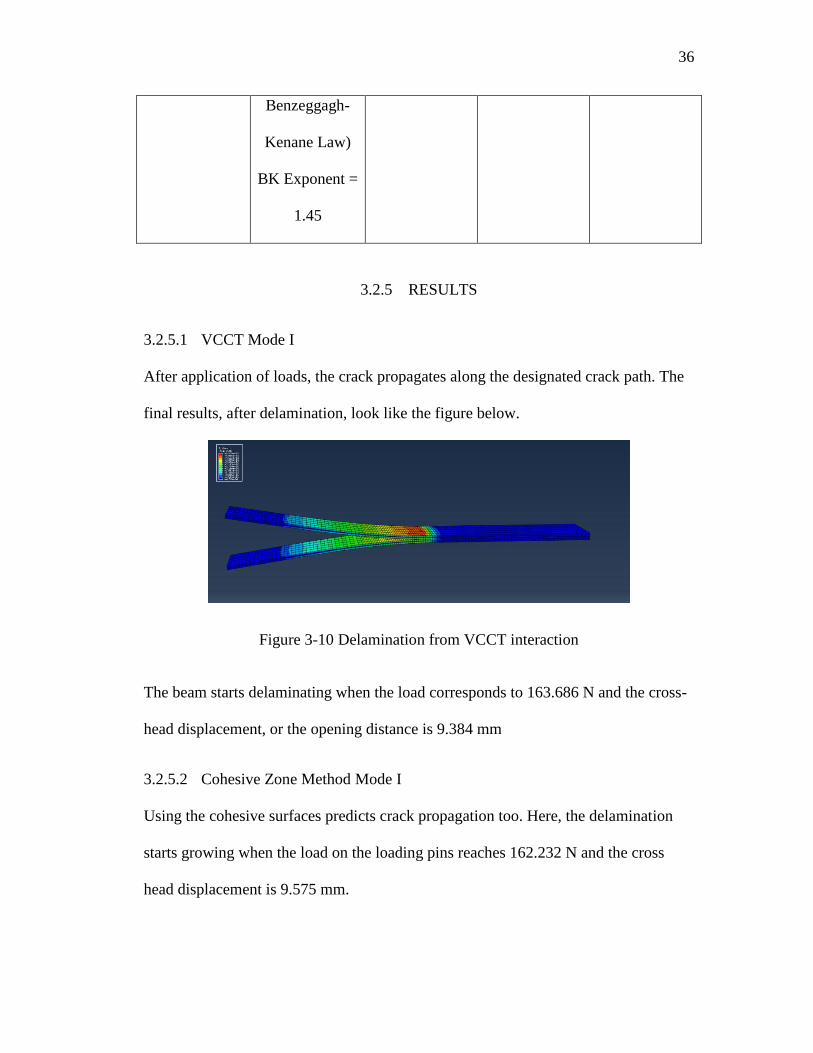
3.2.5.1 VCCT Mode I

After application of loads, the crack propagates along the designated crack path. The

final results, after delamination, look like the figure below.

Figure 3-10 Delamination from VCCT interaction

The beam starts delaminating when the load corresponds to 163.686 N and the cross-

head displacement, or the opening distance is 9.384 mm

3.2.5.2 Cohesive Zone Method Mode I

Using the cohesive surfaces predicts crack propagation too. Here, the delamination

starts growing when the load on the loading pins reaches 162.232 N and the cross

head displacement is 9.575 mm.

37

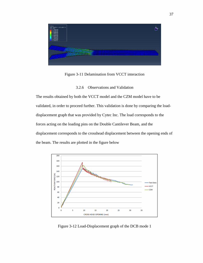
Figure 3-11 Delamination from VCCT interaction

3.2.6 Observations and Validation

The results obtained by both the VCCT model and the CZM model have to be

validated, in order to proceed further. This validation is done by comparing the load-

displacement graph that was provided by Cytec Inc. The load corresponds to the

forces acting on the loading pins on the Double Cantilever Beam, and the

displacement corresponds to the crosshead displacement between the opening ends of

the beam. The results are plotted in the figure below

Figure 3-12 Load-Displacement graph of the DCB mode 1

38

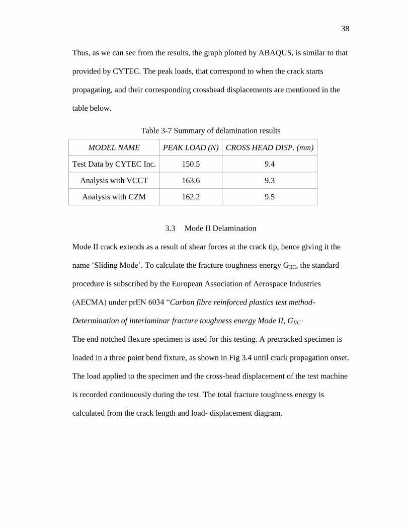
Thus, as we can see from the results, the graph plotted by ABAQUS, is similar to that

provided by CYTEC. The peak loads, that correspond to when the crack starts

propagating, and their corresponding crosshead displacements are mentioned in the

table below.

Table 3-7 Summary of delamination results

MODEL NAME PEAK LOAD (N) CROSS HEAD DISP. (mm)

Test Data by CYTEC Inc. 150.5 9.4

Analysis with VCCT 163.6 9.3

Analysis with CZM 162.2 9.5

3.3 Mode II Delamination

Mode II crack extends as a result of shear forces at the crack tip, hence giving it the

name ‘Sliding Mode’. To calculate the fracture toughness energy GIIC, the standard

procedure is subscribed by the European Association of Aerospace Industries

(AECMA) under prEN 6034 “Carbon fibre reinforced plastics test method-

Determination of interlaminar fracture toughness energy Mode II, GIIC”

The end notched flexure specimen is used for this testing. A precracked specimen is

loaded in a three point bend fixture, as shown in Fig 3.4 until crack propagation onset.

The load applied to the specimen and the cross-head displacement of the test machine

is recorded continuously during the test. The total fracture toughness energy is

calculated from the crack length and load- displacement diagram.

39

Figure 3-13 Standard test specimen for EN6034

Figure 3-14 Test fixture

3.3.1 Experimental procedure and Cytec Results

To achieve reproducible test results, the procedure as specified on pEN6034 has to be

followed. The initial crack lengths must be accurately measured and the continuous

40

load-displacement record must be made, measuring the displacement of the loading

nose.

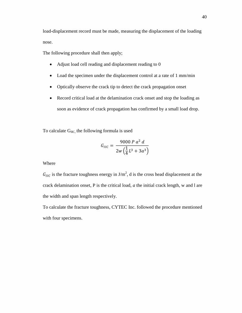
The following procedure shall then apply;

Adjust load cell reading and displacement reading to 0

Load the specimen under the displacement control at a rate of 1 mm/min

Optically observe the crack tip to detect the crack propagation onset

Record critical load at the delamination crack onset and stop the loading as

soon as evidence of crack propagation has confirmed by a small load drop.

To calculate GIIC, the following formula is used

𝐺𝐼𝐼𝐶 = 9000 𝑃 𝑎2 𝑑

2𝑤 (14 𝐿3 + 3𝑎3)

Where

𝐺𝐼𝐼𝐶 is the fracture toughness energy in J/m2, d is the cross head displacement at the

crack delamination onset, P is the critical load, a the initial crack length, w and l are

the width and span length respectively.

To calculate the fracture toughness, CYTEC Inc. followed the procedure mentioned

with four specimens.

41

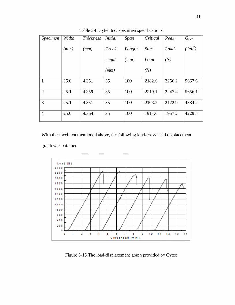
Table 3-8 Cytec Inc. specimen specifications

Specimen Width

(mm)

Thickness

(mm)

Initial

Crack

length

(mm)

Span

Length

(mm)

Critical

Start

Load

(N)

Peak

Load

(N)

GIIC

(J/m2)

1 25.0 4.351 35 100 2182.6 2256.2 5667.6

2 25.1 4.359 35 100 2219.1 2247.4 5656.1

3 25.1 4.351 35 100 2103.2 2122.9 4884.2

4 25.0 4/354 35 100 1914.6 1957.2 4229.5

With the specimen mentioned above, the following load-cross head displacement

graph was obtained.

Figure 3-15 The load-displacement graph provided by Cytec

42

3.3.2 Abaqus CAE Model

Figure 3-16 Abaqus CAE model for EN 6034

The above figure shows the ABAQUS model of the Mode II delamination set up. The

set up consists of four parts: The central beam, with the delamination, two support

beams and the loading pin. The beam is made of C/PEKK thermoplastic and the pins

from steel.

Table 3-9 Physical properties of the model

Property Value

Length 110 mm

Width 25 mm


# Plies 30 -

Layup [0]30 -

Initial Delamination 35 mm

Loading Pin diameter 25 mm

Support Pin diameter 10 mm

43

3.3.3 Material Properties

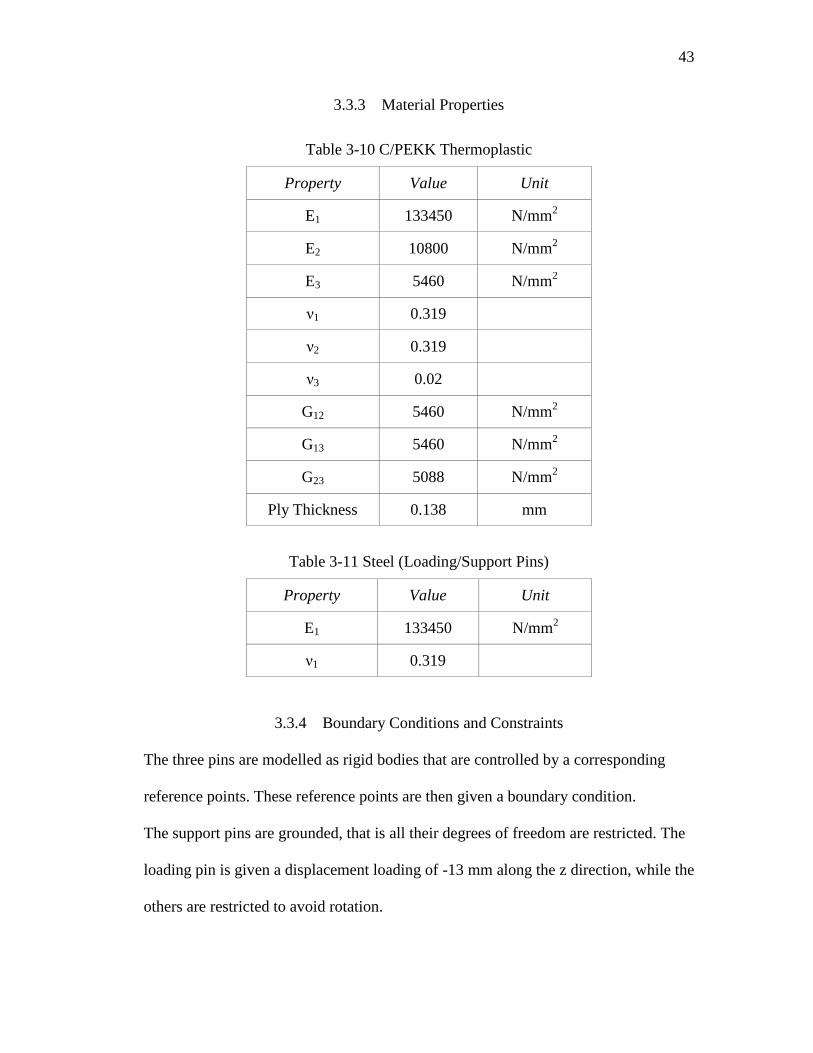
Table 3-10 C/PEKK Thermoplastic

Property Value Unit

E1 133450 N/mm2

E2 10800 N/mm2

E3 5460 N/mm2

ν1 0.319

ν2 0.319

ν3 0.02

G12 5460 N/mm2

G13 5460 N/mm2

G23 5088 N/mm2


Table 3-11 Steel (Loading/Support Pins)

Property Value Unit

E1 133450 N/mm2

ν1 0.319

3.3.4 Boundary Conditions and Constraints

The three pins are modelled as rigid bodies that are controlled by a corresponding

reference points. These reference points are then given a boundary condition.

The support pins are grounded, that is all their degrees of freedom are restricted. The

loading pin is given a displacement loading of -13 mm along the z direction, while the

others are restricted to avoid rotation.

44

Figure 3-17 Support and Loading Pins modeled as rigid bodies

Table 3-12 Boundary Conditions for Mode II delamination setup

Reference Point U1 U2 U3

1 (loading) 0 0 -13

2 (support) 0 0 0

3 (support) 0 0 0

3.3.5 Interactions

Interactions are inserted mid-plane in the beam, where the pre crack lies and the crack

will propagate. This interaction can be VCCT or CZM, with the same properties as

mentioned in the previous section.

45

Figure 3-18 Mid-plane interaction mode II

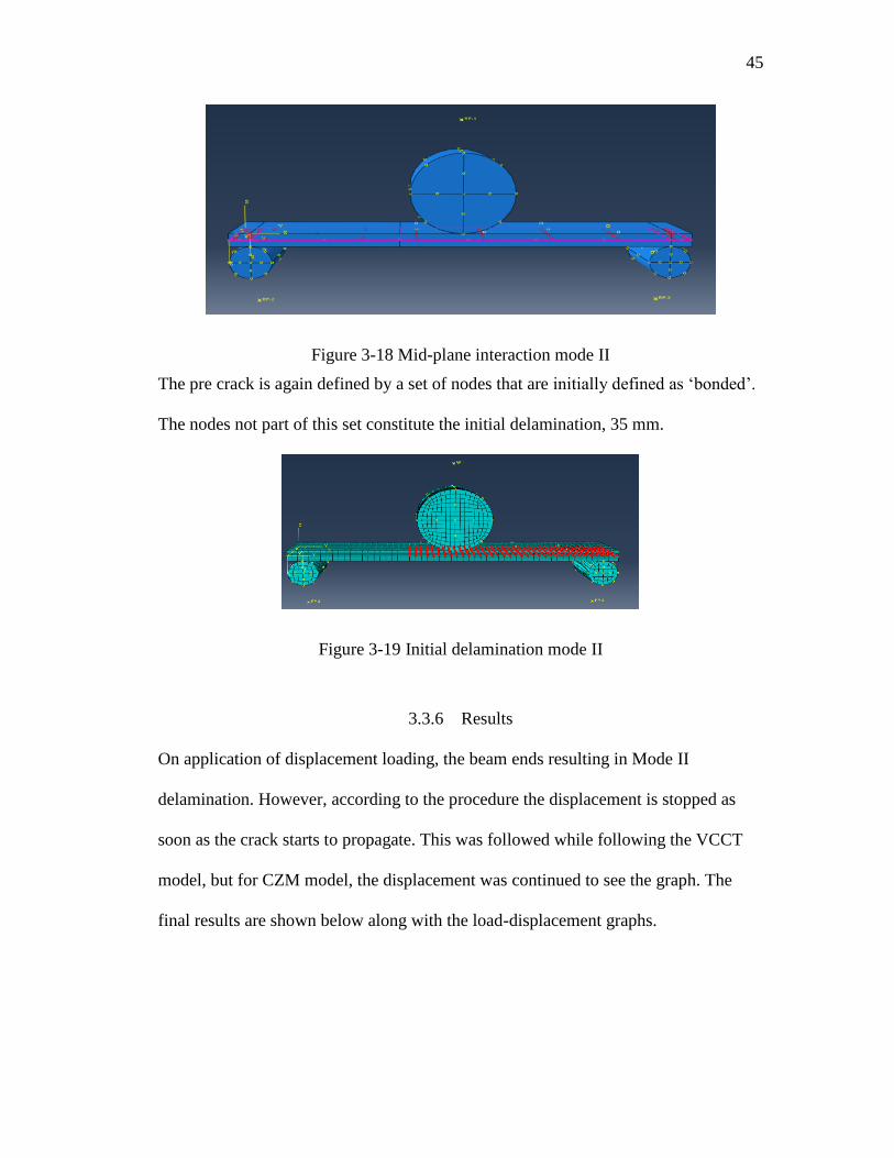
The pre crack is again defined by a set of nodes that are initially defined as ‘bonded’.

The nodes not part of this set constitute the initial delamination, 35 mm.

Figure 3-19 Initial delamination mode II

3.3.6 Results

On application of displacement loading, the beam ends resulting in Mode II

delamination. However, according to the procedure the displacement is stopped as

soon as the crack starts to propagate. This was followed while following the VCCT

model, but for CZM model, the displacement was continued to see the graph. The

final results are shown below along with the load-displacement graphs.

46

3.3.6.1 VCCT Model

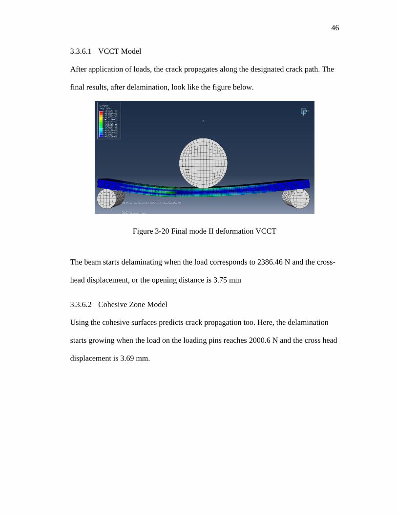
After application of loads, the crack propagates along the designated crack path. The

final results, after delamination, look like the figure below.

Figure 3-20 Final mode II deformation VCCT

The beam starts delaminating when the load corresponds to 2386.46 N and the cross-

head displacement, or the opening distance is 3.75 mm

3.3.6.2 Cohesive Zone Model

Using the cohesive surfaces predicts crack propagation too. Here, the delamination

starts growing when the load on the loading pins reaches 2000.6 N and the cross head

displacement is 3.69 mm.

47

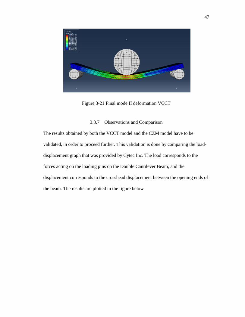
Figure 3-21 Final mode II deformation VCCT

3.3.7 Observations and Comparison

The results obtained by both the VCCT model and the CZM model have to be

validated, in order to proceed further. This validation is done by comparing the load-

displacement graph that was provided by Cytec Inc. The load corresponds to the

forces acting on the loading pins on the Double Cantilever Beam, and the

displacement corresponds to the crosshead displacement between the opening ends of

the beam. The results are plotted in the figure below

48

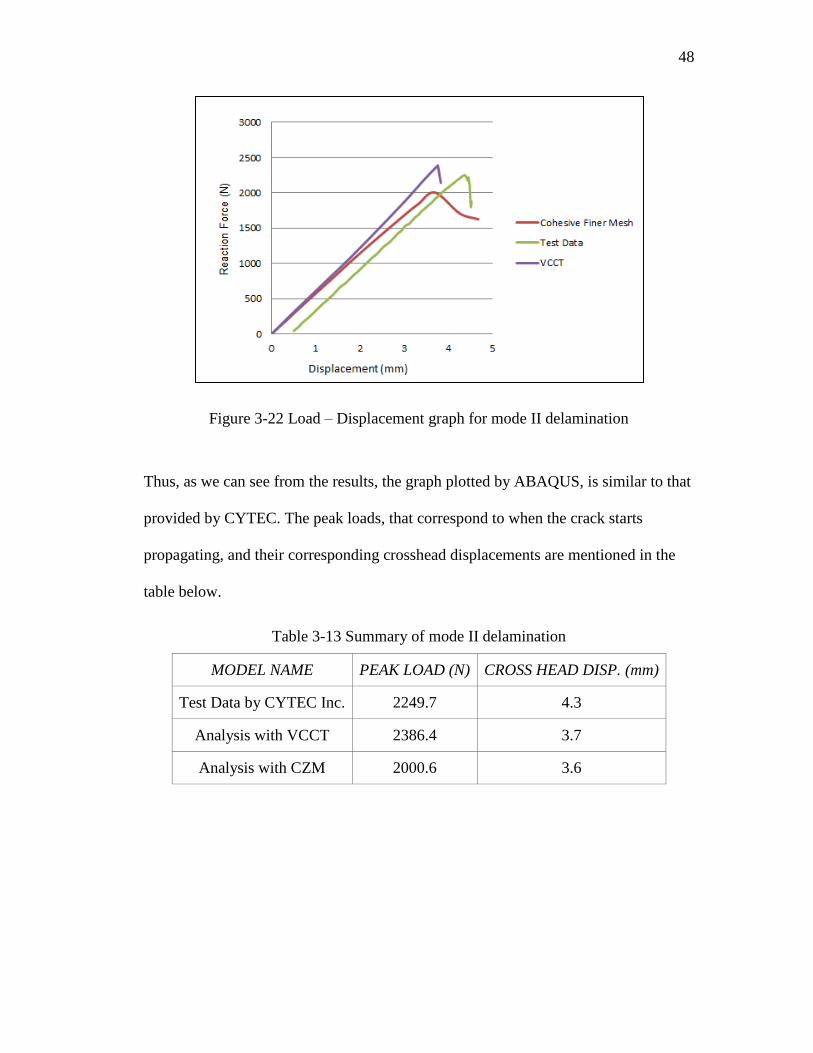
Figure 3-22 Load – Displacement graph for mode II delamination

Thus, as we can see from the results, the graph plotted by ABAQUS, is similar to that

provided by CYTEC. The peak loads, that correspond to when the crack starts

propagating, and their corresponding crosshead displacements are mentioned in the

table below.

Table 3-13 Summary of mode II delamination

MODEL NAME PEAK LOAD (N) CROSS HEAD DISP. (mm)

Test Data by CYTEC Inc. 2249.7 4.3

Analysis with VCCT 2386.4 3.7

Analysis with CZM 2000.6 3.6

49

CHAPTER 4. MODELING FOUR POINT BEND TEST OF THE I-BEAM

This section documents the damage tolerance analysis performed on a 3-stringer test

panel, which is to be tested as part of the TAPAS technology development program.

The skin and stringers are made from thermoplastic composite material (Carbon /

PEKK) and joined with a butt-joint connection between stringer web and skin.

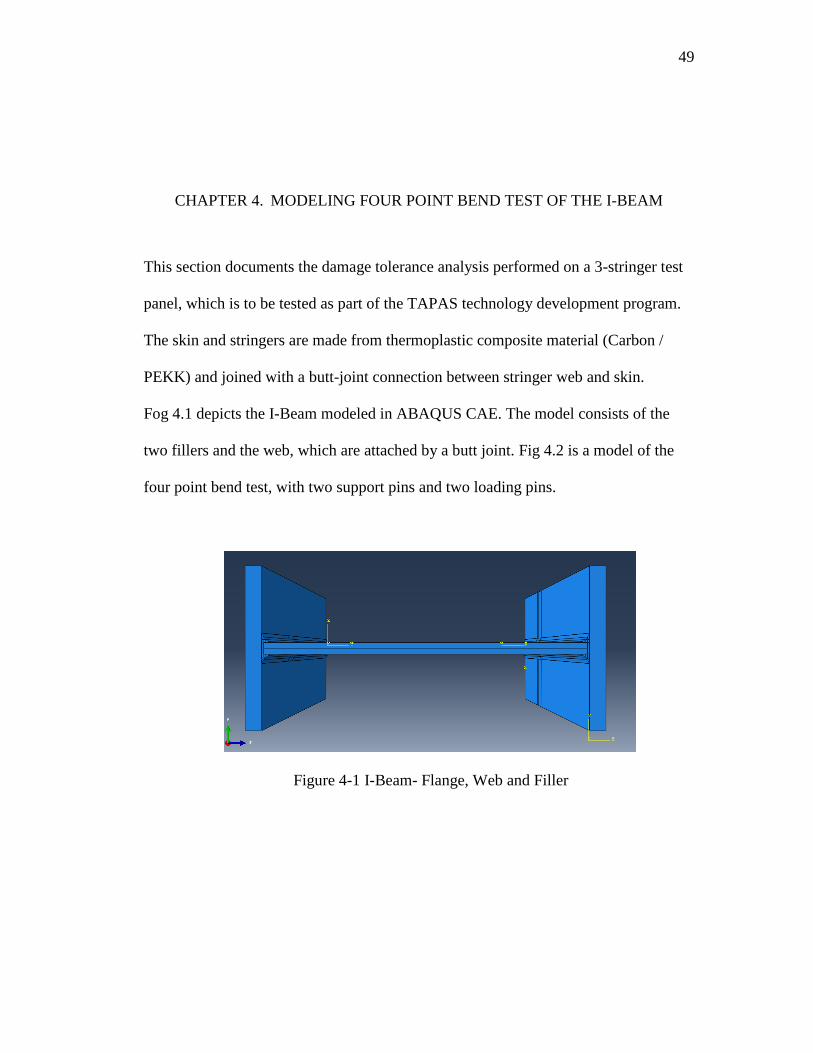
Fog 4.1 depicts the I-Beam modeled in ABAQUS CAE. The model consists of the

two fillers and the web, which are attached by a butt joint. Fig 4.2 is a model of the

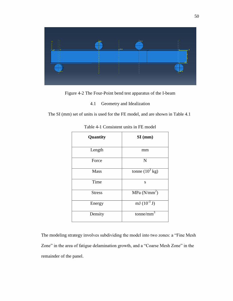
four point bend test, with two support pins and two loading pins.

Figure 4-1 I-Beam- Flange, Web and Filler

50

Figure 4-2 The Four-Point bend test apparatus of the I-beam

4.1 Geometry and Idealization

The SI (mm) set of units is used for the FE model, and are shown in Table 4.1

Table 4-1 Consistent units in FE model

Quantity SI (mm)

Length mm

Force N

Mass tonne (103 kg)

Time s

Stress MPa (N/mm2)

Energy mJ (10-3

J)

Density tonne/mm3

The modeling strategy involves subdividing the model into two zones: a “Fine Mesh

Zone” in the area of fatigue delamination growth, and a “Coarse Mesh Zone” in the

remainder of the panel.

51

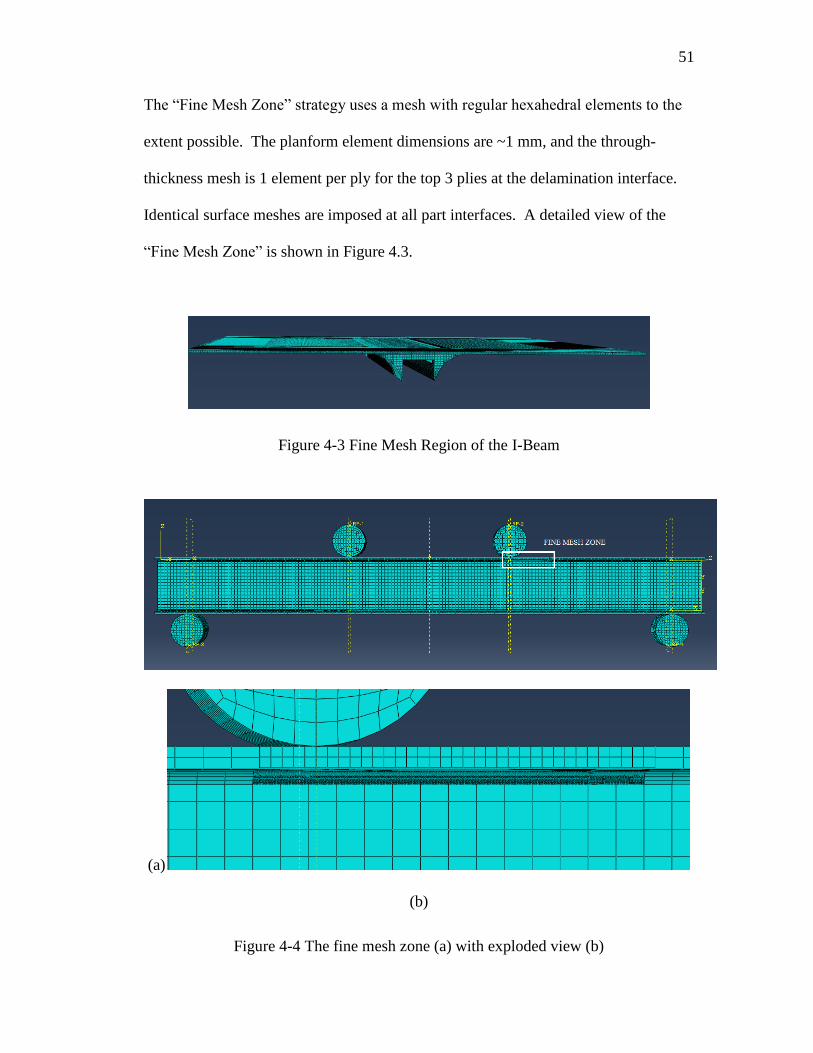
The “Fine Mesh Zone” strategy uses a mesh with regular hexahedral elements to the

extent possible. The planform element dimensions are ~1 mm, and the through-

thickness mesh is 1 element per ply for the top 3 plies at the delamination interface.

Identical surface meshes are imposed at all part interfaces. A detailed view of the

“Fine Mesh Zone” is shown in Figure 4.3.

Figure 4-3 Fine Mesh Region of the I-Beam

(a)

(b)

Figure 4-4 The fine mesh zone (a) with exploded view (b)

52

The “Coarse Mesh Zone” strategy uses a relatively coarse mesh (sufficient to capture

the panel stiffness and stability response). The planform element dimensions are ~4 –

10 mm and 2 element through the thickness of each structural member. The

ABAQUS surface “tying” strategy is used to connect the Coarse Mesh Zone to the

Fine Mesh Zone.

4.1.1 Fine Mesh Filler

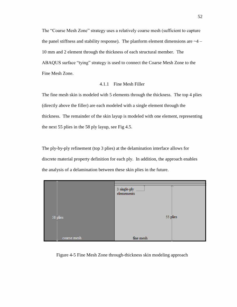
The fine mesh skin is modeled with 5 elements through the thickness. The top 4 plies

(directly above the filler) are each modeled with a single element through the

thickness. The remainder of the skin layup is modeled with one element, representing

the next 55 plies in the 58 ply layup, see Fig 4.5.

The ply-by-ply refinement (top 3 plies) at the delamination interface allows for

discrete material property definition for each ply. In addition, the approach enables

the analysis of a delamination between these skin plies in the future.

Figure 4-5 Fine Mesh Zone through-thickness skin modeling approach

53

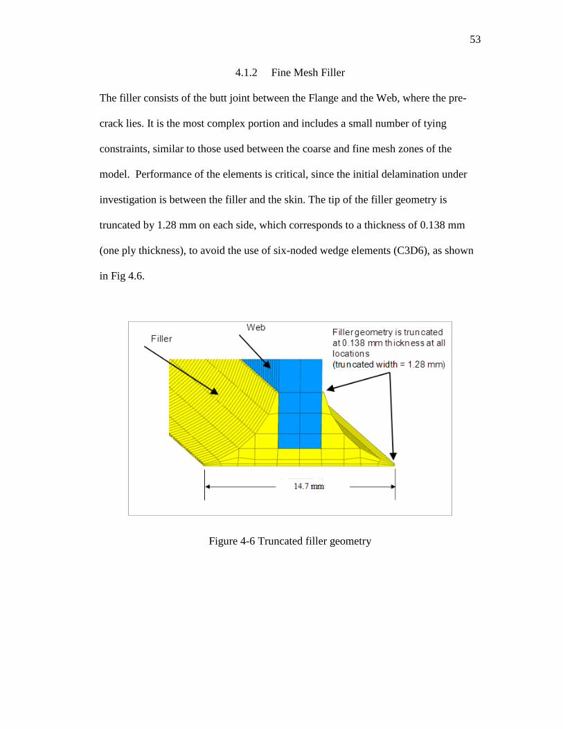
4.1.2 Fine Mesh Filler

The filler consists of the butt joint between the Flange and the Web, where the pre-

crack lies. It is the most complex portion and includes a small number of tying

constraints, similar to those used between the coarse and fine mesh zones of the

model. Performance of the elements is critical, since the initial delamination under

investigation is between the filler and the skin. The tip of the filler geometry is

truncated by 1.28 mm on each side, which corresponds to a thickness of 0.138 mm

(one ply thickness), to avoid the use of six-noded wedge elements (C3D6), as shown

in Fig 4.6.

Figure 4-6 Truncated filler geometry

54

Figure 4-7 Fine mesh zone of the filler length

4.2 Material Properties

The material properties used in the analysis are shown in table 4.2 through table 4.4.

Material properties for the ASD4/PEKK material were supplied by Fokker, in

coordination memos and email correspondence. Material properties for aluminum

were defined as “Typical” industry values.

Table 4-2 3D Ply Properties for ASD4/PEKK

Property Value Unit

E1 133450 N/mm2

E2 10800 N/mm2

E3 5460 N/mm2

ν1 0.319

ν2 0.319

ν3 0.02

G12 5460 N/mm2

G13 5460 N/mm2

G23 5088 N/mm2


55

Table 4-3 Properties for Filler

Property Value Unit

E 1.31 * 104

N/mm2

ν 0.4

Table 4-4 Properties of Steel (Loading/Support Pins)

Property Value Unit

E 2 * 105 N/mm

2

ν 0.3

4.3 Laminate Definitions

Laminate definitions for the coarse mesh region of the FE model use the ABAQUS

*SOLID SECTION, COMPOSITE, option. This input option uses a ply-by-ply

definition of the laminate stack. Laminate definitions for the fine mesh stringer also

use the ABAQUS *SOLID SECTION, COMPOSITE option. The fine mesh skin

region uses individual elements for the first 3 IML plies and 3 elements for the next

55 plies in the 58-ply layup. Properties for the first 3 IML plies are defined in the

fiber direction and rotated to the appropriate angle using the *ORIENTATION option.

Properties for the remainder of the sub-laminate are defined with the *SOLID

SECTION, COMPOSITE option.

Laminate definitions for the flange and web are given in table 4.5. Note: The 0°

fiber direction is aligned with the global axial X direction.

56

Table 4-5 Layup Definitions for I-Beam

Section Source Layup

Flange – 58 Ply TW-14-086

-45/0/0/45/90/90/-45/0/-45/0/45/90/45/90/-

45/0/45/90/-45/0/45/90/-45/0/45/90/-

45/45/0/90/45/-45/90/45/0/-45/90/45/0/-

45/90/45/0/-45/90/45/90/45/0/-45/0/-

45/90/90/45/0/0/0

Web – 40 Ply TW-14-086

[-45/90/45/0/-45/90/45/0/-45/90/45/0/-

45/90/45/0/-45/90/45/0]s

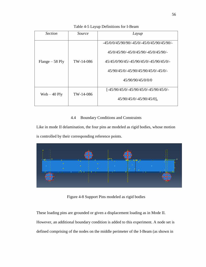
4.4 Boundary Conditions and Constraints

Like in mode II delamination, the four pins ae modeled as rigid bodies, whose motion

is controlled by their corresponding reference points.

Figure 4-8 Support Pins modeled as rigid bodies

These loading pins are grounded or given a displacement loading as in Mode II.

However, an additional boundary condition is added to this experiment. A node set is

defined comprising of the nodes on the middle perimeter of the I-Beam (as shown in

57

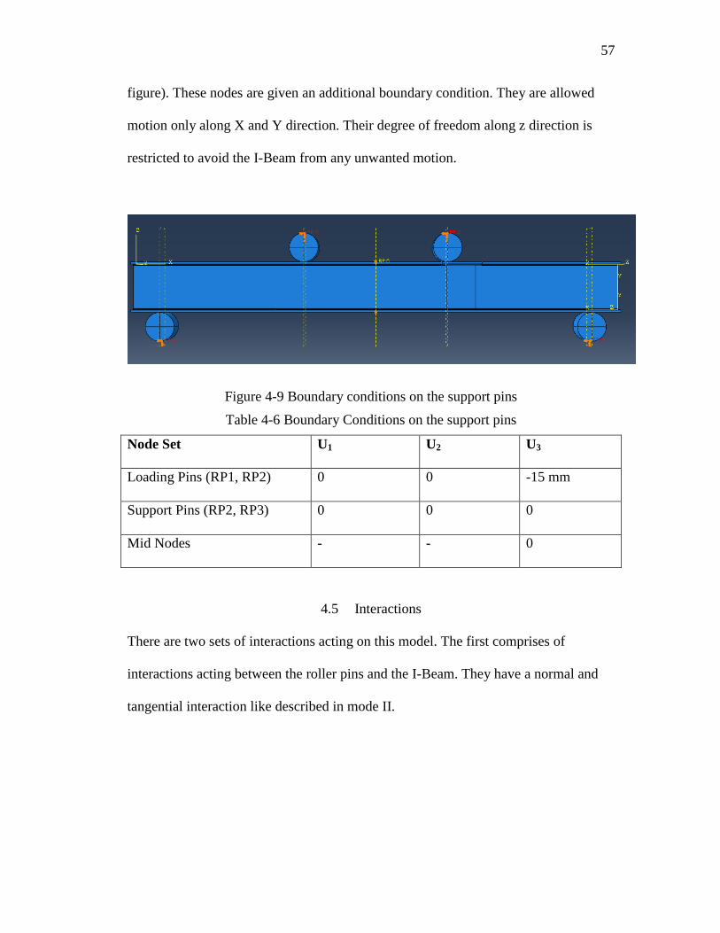
figure). These nodes are given an additional boundary condition. They are allowed

motion only along X and Y direction. Their degree of freedom along z direction is

restricted to avoid the I-Beam from any unwanted motion.

Figure 4-9 Boundary conditions on the support pins

Table 4-6 Boundary Conditions on the support pins

Node Set U1 U2 U3

Loading Pins (RP1, RP2) 0 0 -15 mm

Support Pins (RP2, RP3) 0 0 0

Mid Nodes - - 0

4.5 Interactions

There are two sets of interactions acting on this model. The first comprises of

interactions acting between the roller pins and the I-Beam. They have a normal and

tangential interaction like described in mode II.

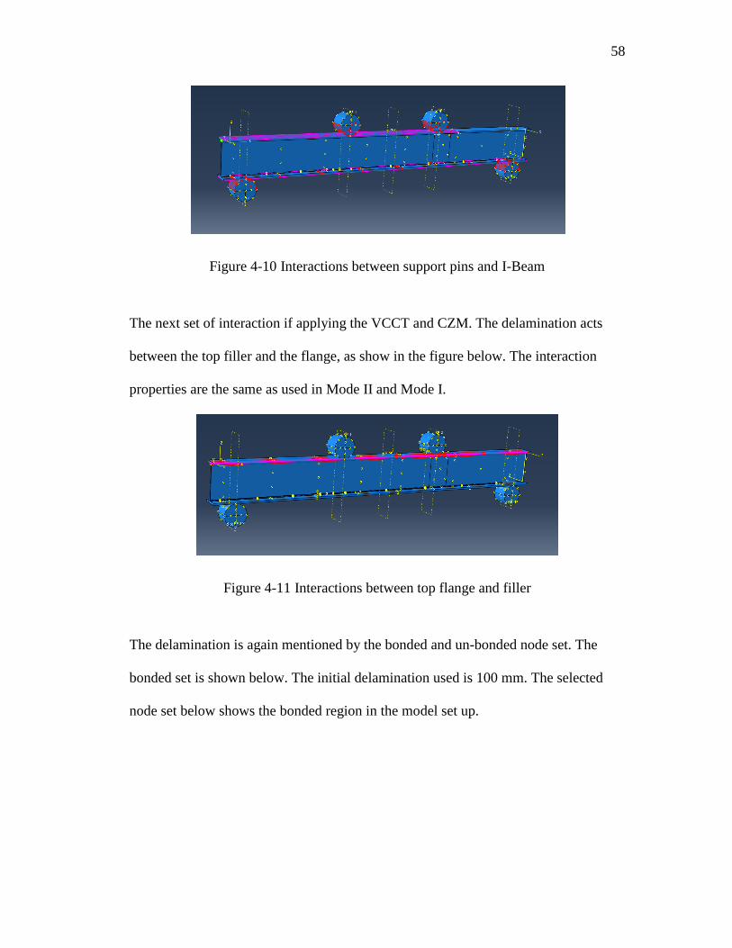
58

Figure 4-10 Interactions between support pins and I-Beam

The next set of interaction if applying the VCCT and CZM. The delamination acts

between the top filler and the flange, as show in the figure below. The interaction

properties are the same as used in Mode II and Mode I.

Figure 4-11 Interactions between top flange and filler

The delamination is again mentioned by the bonded and un-bonded node set. The

bonded set is shown below. The initial delamination used is 100 mm. The selected

node set below shows the bonded region in the model set up.

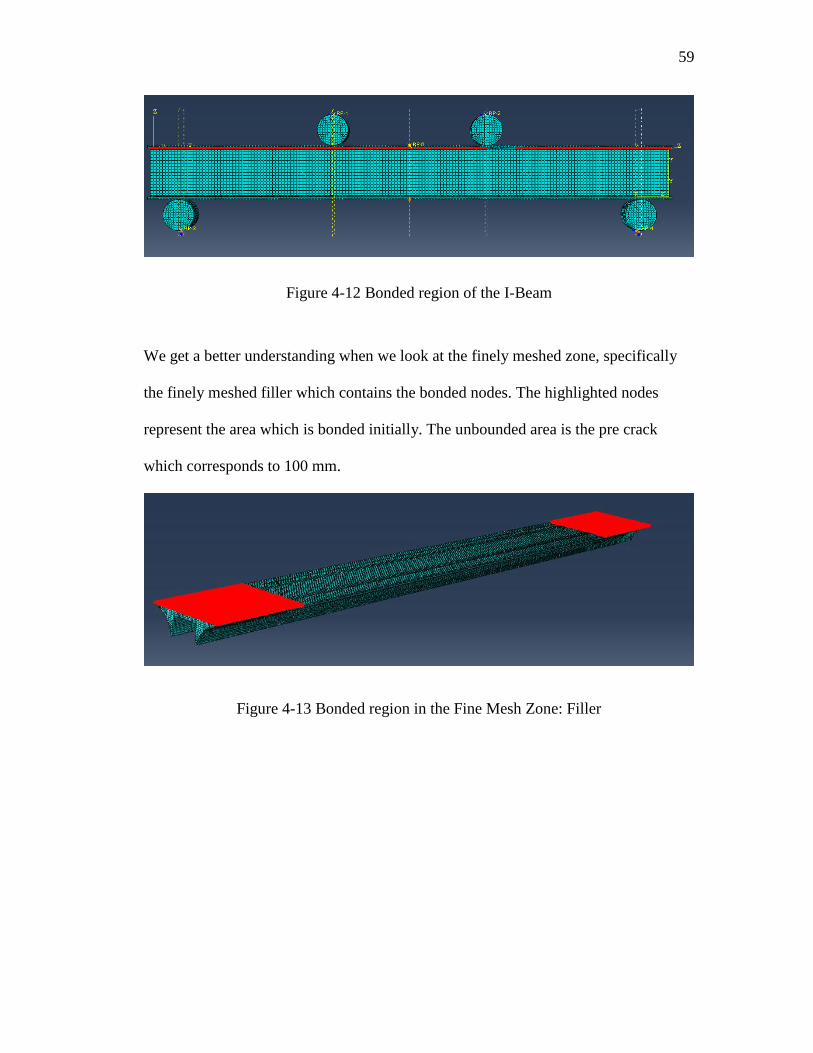
59

Figure 4-12 Bonded region of the I-Beam

We get a better understanding when we look at the finely meshed zone, specifically

the finely meshed filler which contains the bonded nodes. The highlighted nodes

represent the area which is bonded initially. The unbounded area is the pre crack

which corresponds to 100 mm.

Figure 4-13 Bonded region in the Fine Mesh Zone: Filler

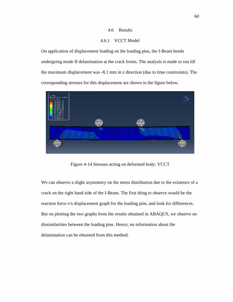
60

4.6 Results

4.6.1 VCCT Model

On application of displacement loading on the loading pins, the I-Beam bends

undergoing mode II delamination at the crack fronts. The analysis is made to run till

the maximum displacement was -8.1 mm in z direction (due to time constraints). The

corresponding stresses for this displacement are shown in the figure below.

Figure 4-14 Stresses acting on deformed body: VCCT

We can observe a slight asymmetry on the stress distribution due to the existence of a

crack on the right hand side of the I-Beam. The first thing to observe would be the

reaction force v/s displacement graph for the loading pins, and look for differences.

But on plotting the two graphs from the results obtained in ABAQUS, we observe no

dissimilarities between the loading pins. Hence, no information about the

delamination can be obtained from this method.

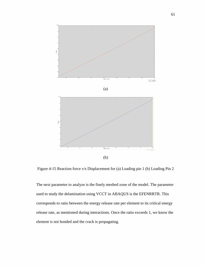
61

(a)

(b)

Figure 4-15 Reaction force v/s Displacement for (a) Loading pin 1 (b) Loading Pin 2

The next parameter to analyze is the finely meshed zone of the model. The parameter

used to study the delamination using VCCT in ABAQUS is the EFENRRTR. This

corresponds to ratio between the energy release rate per element to its critical energy

release rate, as mentioned during interactions. Once the ratio exceeds 1, we know the

element is not bonded and the crack is propagating.

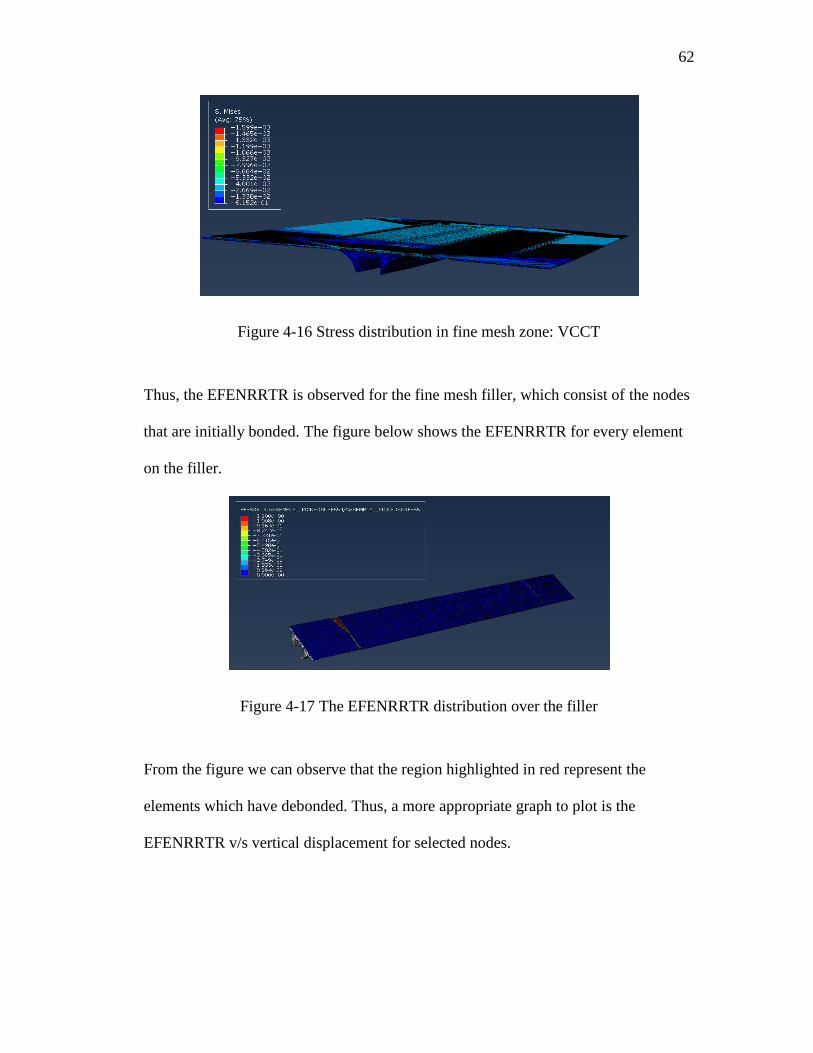
62

Figure 4-16 Stress distribution in fine mesh zone: VCCT

Thus, the EFENRRTR is observed for the fine mesh filler, which consist of the nodes

that are initially bonded. The figure below shows the EFENRRTR for every element

on the filler.

Figure 4-17 The EFENRRTR distribution over the filler

From the figure we can observe that the region highlighted in red represent the

elements which have debonded. Thus, a more appropriate graph to plot is the

EFENRRTR v/s vertical displacement for selected nodes.

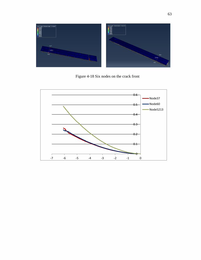
63

Figure 4-18 Six nodes on the crack front

0

0.1

0.2

0.3

0.4

0.5

0.6

-7 -6 -5 -4 -3 -2 -1 0

Node37

Node60

Node5213

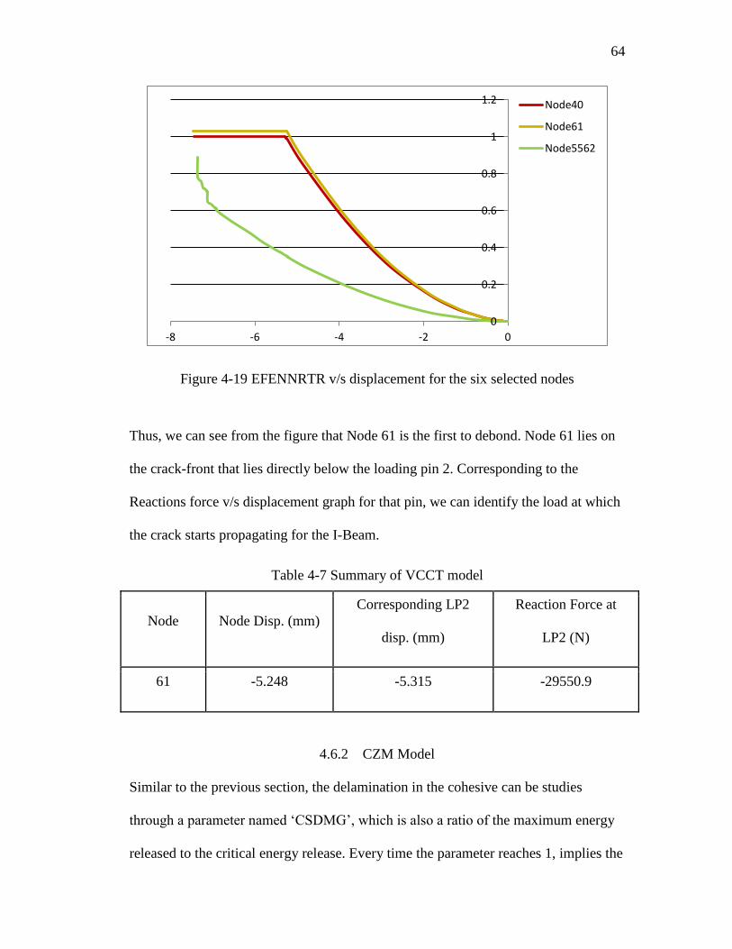
64

Figure 4-19 EFENNRTR v/s displacement for the six selected nodes

Thus, we can see from the figure that Node 61 is the first to debond. Node 61 lies on

the crack-front that lies directly below the loading pin 2. Corresponding to the

Reactions force v/s displacement graph for that pin, we can identify the load at which

the crack starts propagating for the I-Beam.

Table 4-7 Summary of VCCT model

Node Node Disp. (mm)

Corresponding LP2

disp. (mm)

Reaction Force at

LP2 (N)

61 -5.248 -5.315 -29550.9

4.6.2 CZM Model

Similar to the previous section, the delamination in the cohesive can be studies

through a parameter named ‘CSDMG’, which is also a ratio of the maximum energy

released to the critical energy release. Every time the parameter reaches 1, implies the

0

0.2

0.4

0.6

0.8

1

1.2

-8 -6 -4 -2 0

Node40

Node61

Node5562

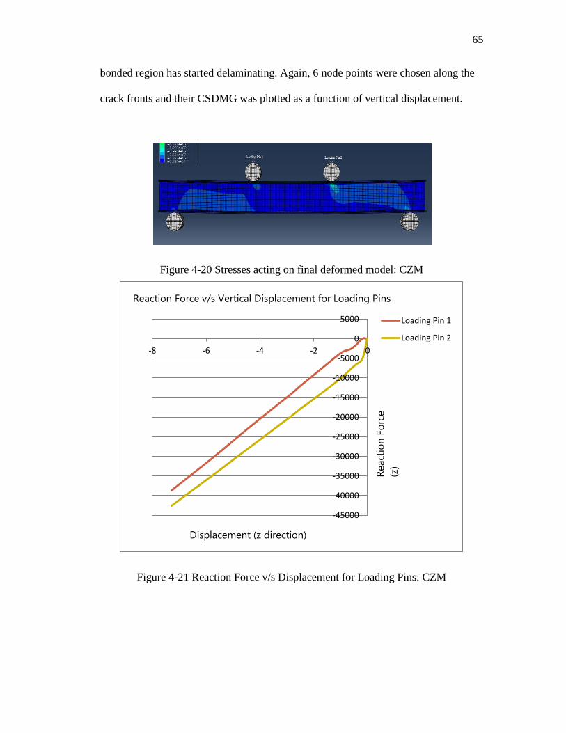
65

bonded region has started delaminating. Again, 6 node points were chosen along the

crack fronts and their CSDMG was plotted as a function of vertical displacement.

Figure 4-20 Stresses acting on final deformed model: CZM

Figure 4-21 Reaction Force v/s Displacement for Loading Pins: CZM

-45000

-40000

-35000

-30000

-25000

-20000

-15000

-10000

-5000

0

5000

-8 -6 -4 -2 0

Loading Pin 1

Loading Pin 2

Reaction Force v/s Vertical Displacement for Loading Pins

React

ion

Fo

rce

(z)

Displacement (z direction)

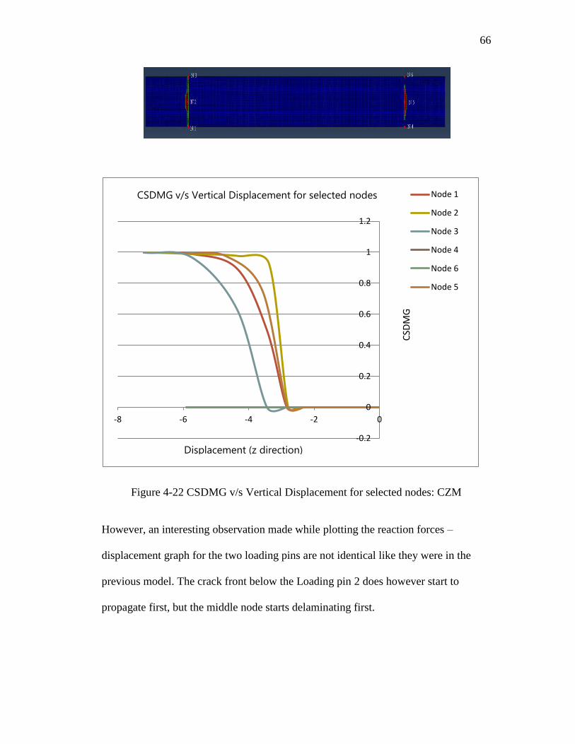
66

Figure 4-22 CSDMG v/s Vertical Displacement for selected nodes: CZM

However, an interesting observation made while plotting the reaction forces –

displacement graph for the two loading pins are not identical like they were in the

previous model. The crack front below the Loading pin 2 does however start to

propagate first, but the middle node starts delaminating first.

-0.2

0

0.2

0.4

0.6

0.8

1

1.2

-8 -6 -4 -2 0

Node 1

Node 2

Node 3

Node 4

Node 6

Node 5

CSDMG v/s Vertical Displacement for selected nodes


CSD

MG

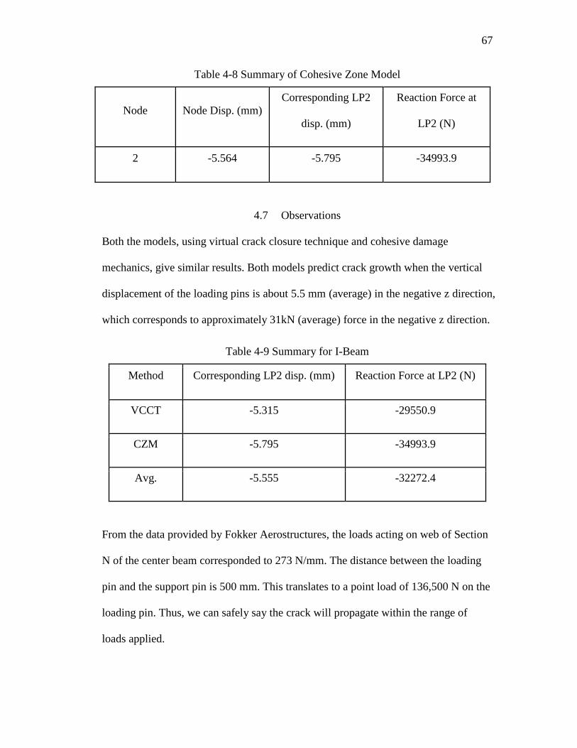
67

Table 4-8 Summary of Cohesive Zone Model

Node Node Disp. (mm)

Corresponding LP2

disp. (mm)

Reaction Force at

LP2 (N)

2 -5.564 -5.795 -34993.9

4.7 Observations

Both the models, using virtual crack closure technique and cohesive damage

mechanics, give similar results. Both models predict crack growth when the vertical

displacement of the loading pins is about 5.5 mm (average) in the negative z direction,

which corresponds to approximately 31kN (average) force in the negative z direction.

Table 4-9 Summary for I-Beam

Method Corresponding LP2 disp. (mm) Reaction Force at LP2 (N)

VCCT -5.315 -29550.9

CZM -5.795 -34993.9

Avg. -5.555 -32272.4

From the data provided by Fokker Aerostructures, the loads acting on web of Section

N of the center beam corresponded to 273 N/mm. The distance between the loading

pin and the support pin is 500 mm. This translates to a point load of 136,500 N on the

loading pin. Thus, we can safely say the crack will propagate within the range of

loads applied.

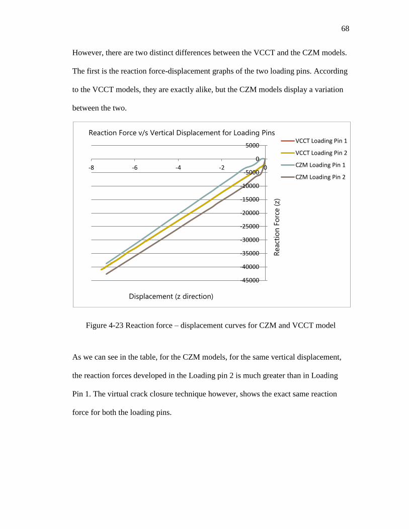
68

However, there are two distinct differences between the VCCT and the CZM models.

The first is the reaction force-displacement graphs of the two loading pins. According

to the VCCT models, they are exactly alike, but the CZM models display a variation

between the two.

Figure 4-23 Reaction force – displacement curves for CZM and VCCT model

As we can see in the table, for the CZM models, for the same vertical displacement,

the reaction forces developed in the Loading pin 2 is much greater than in Loading

Pin 1. The virtual crack closure technique however, shows the exact same reaction

force for both the loading pins.

-45000

-40000

-35000

-30000

-25000

-20000

-15000

-10000

-5000

0

5000

-8 -6 -4 -2 0

VCCT Loading Pin 1

VCCT Loading Pin 2

CZM Loading Pin 1

CZM Loading Pin 2

Reaction Force v/s Vertical Displacement for Loading Pins

React

ion

Fo

rce (

z)


69

Another difference is the location of the crack growth. While Virtual Crack Closure

Technique predicts it to be the nodes at the edge of the filler, Cohesive Zone Model

predicts it to be at the mid points of the filler.

70

CHAPTER 5. CONCLUSION

Today, vast majority of composite materials for aerospace are based on thermoset

materials. However, the second half of the 1980s saw the emergence of a new family

of composite materials, continuous fiber reinforced thermoplastics and for the past

few years, they have significantly matured. Their characteristic offers intriguing

possibilities for both faster and more innovative composite processing techniques

compared to their thermoset counterparts. This lead to the start of the Thermoplastic

Primary Aircraft Structure innovation program (TAPAS), a consortium that consists

of companies and knowledge institutes in the Dutch aerospace industry working

together with the aircraft manufacturer Airbus, which aims to increase the proportion

of thermoplastic composites in commercial aircrafts.

For this thesis, the center beam of the Gulfstream 650 aircraft’s horizontal tail plane,

previously a carbon fiber/epoxy hat-stiffened skin construction is being redesigned

using unidirectional carbon fiber/PEKK (Poly-ether-ketone-ketone) composite. An I-

Beam is modeled with the dimensions of a certain section of the center beam, along

with the loads acting on the carbon epoxy counterpart. However, a pre-crack of 100

mm in inserted in the beam between the top flange and the filler, and a damage

analysis is performed to see if the model delaminates within the load range that acts

on the current carbon fiber/epoxy model.

71

To perform the damage analysis on the I-Beam two finite element methods were

identified, namely Virtual Crack Closure Technique and Cohesive Zone Model.

However, before analyzing the C/PEKK I-Beam, the two methods were first verified

by reproducing the experimental data done by Cytec Inc. for determining the fracture

toughness (G1c and G2c) in pure mode I and mode II delamination. The experiments

followed the standard procedures prescribed by ASTM 5528 for mode I and EN 6034

for mode II bending. To simulate the loading applied on the G650 center beam, the I-

Beam was placed under a four point bend, with a constant displacement loading. The

model was then analyzed to study the forces at which the crack starts growing, using

both VCCT and CZM.

We observe from the results that both finite element approaches produce similar

results, which state that the crack starts to grow when the vertical displacement of the

load pins are about 5.55 mm and have a reaction force corresponding to 32.27 kN.

Thus, considering the loads acting on the carbon fiber/epoxy center beam lie in the

magnitude of 136.5 kN, the thermoplastic model will definitely see crack propagation

if it has an initial delamination.

Thus, to prevent this there are only two parameters that can be tampered with: the

material used and the area of contact between the filler and the flange. The latter

parameter can be increased and the filler can be made wider, to increase the contact

with the flange. However, the most significant conclusion made from the report is the

difference in the modeling cohesive interactions and virtual crack closure technique

72

in ABAQUS. It was observed that the analysis time required for CZM was

significantly lesser than the models using VCCT interactions. With each model

analyzed in this project, its complexity progressively increased. First, there was a

simple beam with opening loads, next a beam under a three point bend and finally an

I-Beam in four-point bend loading condition. With each analysis, the CZM model

took one, three and five hour lesser time to complete the job. Thus, we can infer that

for more complex models, the cohesive approach is much faster and can save hours of

computational time.

Further study can be done on the I-Beam by varying the location and the length of the

initial delamination. A through hole can also be modelled to mirror the carbon epoxy

center beam and the stresses in the I-Beam can be observed.

73

REFERENCES

73

REFERENCES

[1] A. R. Offringa, “Thermoplastic composites—rapid processing applications,”

Compos. Part A Appl. Sci. Manuf., vol. 27, no. 4, pp. 329–336, Jan. 1996.

[2] H. Ning, U. Vaidya, G. M. Janowski, and G. Husman, “Design, manufacture and

analysis of a thermoplastic composite frame structure for mass transit,” Compos.

Struct., vol. 80, no. 1, pp. 105–116, Sep. 2007.

[3] M. Hou, L. Ye, H. J. Lee, and Y. W. Mai, “Manufacture of a carbon-fabric-

reinforced polyetherimide (CF/PEI) composite material,” Compos. Sci. Technol.,

vol. 58, no. 2, pp. 181–190, Jan. 1998.

[4] J. Denault and M. Dumouchel, “Consolidation process of PEEK/carbon composite

for aerospace applications,” Adv. Perform. Mater., 1998.

[5] I. Chang, “PEKK as a new thermoplastic matrix for high-performance

composites,” SAMPE Q.;(United States), 1988.

[6] A. Goldberg, “Screening of matrices and fibers for reinforced thermoplastics

intended for dental applications,” J. Biomed. …, 1994.

[7] E. Wang and T. Gutowski, “Cost comparison between thermoplastic and thermoset

composites,” SAMPE J., 1990.

[8] A. Offringa, “Structural Thermoplastic Aircraft Floor Panels--in Series

Production,” Soc. Adv. Mater. Process …, 1994.

[9] G. Marsh, “Reinforced thermoplastics, the next wave?,” Reinf. Plast., 2014.

[10] P. F. Liu, S. J. Hou, J. K. Chu, X. Y. Hu, C. L. Zhou, Y. L. Liu, J. Y. Zheng, A.

Zhao, and L. Yan, “Finite element analysis of postbuckling and delamination of

composite laminates using virtual crack closure technique,” Compos. Struct., vol.

93, no. 6, pp. 1549–1560, May 2011.

[11] D. Sleight, “Progressive failure analysis methodology for laminated composite

structures,” 1999.

74

[12] M. R. Garnich and V. M. K. Akula, “Review of Degradation Models for

Progressive Failure Analysis of Fiber Reinforced Polymer Composites,” Appl.

Mech. Rev., vol. 62, no. 1, p. 010801, 2009.

[13] P. F. Liu and J. Y. Zheng, “Recent developments on damage modeling and finite

element analysis for composite laminates: A review,” Mater. Des., vol. 31, no. 8,

pp. 3825–3834, Sep. 2010.

[14] V. Ranatunga, “Finite element modeling of delamination crack propagation in

laminated composites,” Proc. World Congr. Eng. …, 2011.

[15] E. Rybicki and M. Kanninen, “A finite element calculation of stress intensity

factors by a modified crack closure integral,” Eng. Fract. Mech., 1977.

[16] I. Raju, “Calculation of strain-energy release rates with higher order and singular

finite elements,” Eng. Fract. Mech., 1987.

[17] G. . Barenblatt, “The formation of equilibrium cracks during brittle fracture.

General ideas and hypotheses. Axially-symmetric cracks,” J. Appl. Math. Mech.,

vol. 23, no. 3, pp. 622–636, Jan. 1959.

[18] D. S. Dugdale, “Yielding of steel sheets containing slits,” J. Mech. Phys. Solids,

vol. 8, no. 2, pp. 100–104, May 1960.

[19] H. Hibbitt, B. Karlsson, and P. Sorensen, “Abaqus Analysis User’s Manual

Version 6.10,” Dassault Systèmes Simulia Corp. Provid. RI, …, 2011.

[20] M. Kachanov, “Effective elastic properties of cracked solids: critical review of

some basic concepts,” Appl. Mech. Rev., 1992.

[21] M. Kachanov, “Elastic solids with many cracks and related problems,” 1993.

[22] H. Chai, C. D. Babcock, and W. G. Knauss, “One dimensional modelling of failure

in laminated plates by delamination buckling,” Int. J. Solids Struct., vol. 17, no.

11, pp. 1069–1083, Jan. 1981.

[23] G. Kardomateas, A. Pelegri, and B. Malik, “Growth of internal delaminations

under cyclic compression in composite plates,” … Mech. Phys. …, 1995.

[24] G. Kardomateas and D. Schmueser, “Buckling and postbuckling of delaminated

composites under compressive loads including transverse shear effects,” AIAA J.,

1988.

75

[25] A. J. Kinloch, Y. Wang, J. G. Williams, and P. Yayla, “The mixed-mode

delamination of fibre composite materials,” Compos. Sci. Technol., vol. 47, no. 3,

pp. 225–237, Jan. 1993.

[26] J. Reeder, “3D mixed-mode delamination fracture criteria–an experimentalist’s

perspective,” 2006.

[27] J. R. Willis, “A comparison of the fracture criteria of griffith and barenblatt,” J.

Mech. Phys. Solids, vol. 15, no. 3, pp. 151–162, May 1967.

[28] A. Hillerborg, M. Modéer, and P.-E. Petersson, “Analysis of crack formation and

crack growth in concrete by means of fracture mechanics and finite elements,”

Cem. Concr. Res., vol. 6, no. 6, pp. 773–781, Nov. 1976.

[29] B. Davidson and W. Zhao, “An accurate mixed-mode delamination failure

criterion for laminated fibrous composites requiring limited experimental input,” J.

Compos. Mater., 2007

Delamination of C/PEKK I-Beam using virtual crack closure ...

Documents

Transcript of Delamination of C/PEKK I-Beam using virtual crack closure ...