Degenerate mixing of plasma waves on cold, magnetizedsingle-species plasmas

M. W. Anderson,1 T. M. O’Neil,1 D. H. E. Dubin,1 and R. W. Gould2

1Physics Department, University of California at San Diego, La Jolla, California 92093, USA2California Institute of Technology, Mail Stop 128-95, Pasadena, California 91103, USA

(Received 3 June 2011; accepted 12 September 2011; published online 24 October 2011)

In the cold-fluid dispersion relation x ¼ xp=½1þ ðk?=kzÞ2�1=2for Trivelpiece-Gould waves on an

infinitely long magnetized plasma cylinder, the transverse and axial wavenumbers appear only in the

combination k?=kz. As a result, for any frequency x < xp, there are infinitely many degenerate

waves, all having the same value of k?=kz. On a cold finite-length plasma column, these degenerate

waves reflect into one another at the ends; thus, each standing-wave normal mode of the bounded

plasma is a mixture of many degenerate waves, not a single standing wave as is often assumed. A

striking feature of the many-wave modes is that the short-wavelength waves often add constructively

along resonance cones given by dz=dr ¼ 6ðx2p=x

2 � 1Þ1=2. Also, the presence of short wavelengths

in the admixture for a predominantly long-wavelength mode enhances the viscous damping beyond

what the single-wave approximation would predict. Here, numerical solutions are obtained for modes

of a cylindrical plasma column with rounded ends. Exploiting the fact that the modes of a spheroidal

plasma are known analytically (the Dubin modes), a perturbation analysis is used to investigate

the mixing of low-order, nearly degenerate Dubin modes caused by small deformations of a plasma

spheroid. VC 2011 American Institute of Physics. [doi:10.1063/1.3646922]

I. BACKGROUND AND SUMMARY OF RESULTS

Figure 1 shows a schematic diagram of a single-species

plasma that is confined in a Penning-Malmberg trap.1 A con-

ducting cylinder is divided into three sections, and the

plasma resides in the central grounded section, with radial

confinement provided by a uniform axial magnetic field

ðB ¼ BzÞ and axial confinement by voltages applied to the

outer sections of the cylinder. These plasmas routinely come

to a state of thermal equilibrium in the trap and are routinely

cooled to the cryogenic temperature range.2 The plasma con-

figuration is then particularly simple; the density is constant

out to some surface of revolution and there drops to zero.3

This paper discusses the normal modes of plasma oscillation

for these cold equilibrium plasmas. Of course, cold-fluid

theory provides a good description of these modes.

At first glance, the problem sounds straightforward: find

the longitudinal modes of oscillation of a uniformly magne-

tized, uniform-density, bounded plasma in cold-fluid theory.

However, we will see that the problem is subtle and that

there is some confusion in the literature.

The origin of the difficulty is the peculiar dispersion

relation for plasma waves in a cold magnetized plasma,

x ¼ kzxpffiffiffiffiffiffiffiffiffiffiffiffiffiffiffik2

z þ k2?

p ; (1)

where x is the wave frequency, xp is the plasma frequency

in the unperturbed plasma, kz is the wavenumber along the

magnetic field, and k? is the wavenumber transverse to the

field. Note that a wave with wavenumbers ðkz; k?Þ has the

same frequency as a wave with wavenumbers ðk0z; k0?Þ if

k0z=k

0? ¼ kz=k? thus, each wave has the same frequency

as infinitely many other waves. Upon reflection from the

boundaries, an incident wave typically mixes with other

waves sharing the same frequency, and consequently, each

normal mode is a complicated many-wave structure.

A toy problem illustrates the issues. Consider a two

dimensional slab of uniform-density plasma that occupies

the bounded domain given by 0 � x � a and 0 � z � b, and

assume a strong magnetic field in the z-direction. The poten-

tial for a mode oscillating with frequency x satisfies the

equation

@2dux

@x2þ 1�

x2p

x2

!@2dux

@z2¼ 0: (2)

Suppose that the plasma is bounded on all sides by a perfect

conductor, the potential is zero at the boundaries. In this

case, a set of normal modes and frequencies is given by

duxðx; zÞ ¼ sinmpx

a

� �sin

npx

b

� �; (3)

xmn ¼ðnp=bÞxpffiffiffiffiffiffiffiffiffiffiffiffiffiffiffiffiffiffiffiffiffiffiffiffiffiffiffiffiffiffiffiffiffiffiffiffiffiffi

ðmp=aÞ2 þ ðnp=bÞ2q ; (4)

where m and n are integers. For any mode ðm; nÞ, there are

an infinite number of exactly degenerate modes ðm0; n0Þwhere n0=m0 ¼ n=m. Each mode can be decomposed into a

pair of waves propagating in opposite directions along the

magnetic field and reflecting at the boundaries, but for this

particular geometry, there is no mixing since the sine func-

tions are orthogonal on the boundary surfaces. However, if

the boundary were deformed, the orthogonality would be

destroyed, and reflections would mix degenerate modes,

yielding more complicated many-wave modes.

1070-664X/2011/18(10)/102113/19/$30.00 VC 2011 American Institute of Physics18, 102113-1

PHYSICS OF PLASMAS 18, 102113 (2011)

It is interesting to construct an alternate representation

of the degenerate modes. For any frequency, the mode

equation (2) admits characteristic solutions of the form

dux ¼ d½z6ðx2p=x

2 � 1Þ1=2xþ c�, where c is an arbitrary

constant. These solutions can be thought of as a line or ray at

slope dz=dx ¼ 6ðx2p=x

2 � 1Þ1=2. For the mode frequencies

given by Eq. (4), an assembly of such rays can be arranged

end to end, so that the assembly closes on itself. The sign of

the ray changes upon reflection from the boundary, so that

the boundary condition on the wall is satisfied. Figure 2

shows a parallelogram-shaped assembly for the degenerate

mode frequency corresponding to n=m ¼ 1. There are an in-

finite number of such parallelograms with sides of different

lengths, and this set is an alternative representation of the

sinusoidal degenerate modes of Eq. (3) for which n=m ¼ 1.

Similar ray-like representations can be constructed for any

other set of degenerate modes—that is, for any other value

of the ratio n=m. Interestingly, if the rectangular plasma

boundary is deformed slightly, all of the degenerate sinusoi-

dal modes are mixed, but a given ray-like mode is only

modified if the boundary is moved at the points at which the

ray makes contact.

This picture is modified somewhat in cylindrical geome-

try. For example, for a uniform-density plasma bounded by a

cylindrical conducting wall at r ¼ a and flat conducting

walls at z ¼ 0 and z ¼ b, the mode degeneracies are only

approximate. Furthermore, the ray-like solutions are replaced

by more complicated functions that are peaked along reso-

nance cones with slope4 dz=dr ¼ 6ðx2p=x

2 � 1Þ1=2. A cru-

cial difference is that the cylindrical functions are not

entirely localized along these cones. Nevertheless, the basic

ideas illustrated by the rectangular toy problem persist. In

numerical studies of the normal modes for a long, cylindrical

plasma column in a Penning-Malmberg trap, we will

find complicated many-wave normal modes, with the waves

often adding to produce conical structures with slope

dz=dr ¼ 6ðx2p=x

2 � 1Þ1=2.

We emphasize that the mixing described here is a low-

temperature phenomenon, requiring that the cold-fluid dis-

persion relation be valid for axial and transverse wavelengths

much shorter than the dimensions of the plasma. The condi-

tion for validity of the cold-fluid dispersion relation is that

ðk2? þ k2

z Þ1=2kD � 1; otherwise, kinetic effects such as Lan-

dau damping modify the dispersion relation, spoiling the

degeneracy that underlies the mixing. Using the laser cooling

technique, experimentalists regularly achieve Debye lengths

that are small compared with the plasma dimensions, and in

this regime, mixing should be observable. For example, a

recent experiment on Mgþ plasmas achieved a temperature

of 10�3 eV at a density of 2� 107 cm�3, corresponding to a

Debye length of 5� 10�3 cm; the plasma radius in this

experiment was on the order of 1 cm.5

With this background, we now return to the discussion

of normal modes for a cold equilibrium plasma in a Penning-

Malmberg trap. An important difference between this prob-

lem and the toy problem is that vacuum separates the plasma

from the conducting wall. For the simple case of a mode

with azimuthal mode number zero, the mode equation is

given by

1

r

@

@rr@dux

@rþ @

@z1�

x2pðr; zÞx2

" #@dux

@z¼ 0; (5)

where x2pðr; zÞ ¼ x2

p ¼ constant inside the plasma and

x2pðr; zÞ ¼ 0 in the vacuum. The mode potential vanishes on

the trap wall and as z! 61:Historically, two geometrical limits have been empha-

sized. In the first limit, pioneered by the atomic physics com-

munity, the plasma is small compared to the radius of the

cylindrical conductor and resides in a quadratic trap poten-

tial. The surface of revolution defining the shape of the

plasma is spheroidal in this limit.6 Using spheroidal coordi-

nates, exact analytic expressions for the normal modes can

be found, and images of modes in Beþ plasmas corroborate

these results.7,8 However, these modes have many near

degeneracies, and one expects that a deformation of the

spheroidal boundary will mix these modes.

In the second limit, more familiar to plasma physicists,

the plasma is long compared to the radius of the conducting

cylinder and takes the shape of a finite-length cylinder with

rounded ends. The more complicated shape of these longer

plasmas prevents an analytic description of the modes. How-

ever, the solution by Trivelpiece and Gould (TG) for waves

on a cold, magnetized, infinitely long plasma cylinder

provides a useful benchmark for theoretical studies of modes

FIG. 2. An example of a ray-like mode on a magnetized plasma slab of rec-

tangular cross-section, surrounded by a perfect conductor. The mode poten-

tial is a sum of four Dirac delta functions, each of which is peaked along one

side of the dashed parallelogram. Delta functions corresponding to adjacent

sides enter the sum with opposite signs so that the condition of vanishing

potential is satisfied along the boundary. There are an infinite number of

other ray-like modes with the same frequency as the mode depicted here.

The set of ray-like modes is complimentary to the set of modes that are sinu-

soidal in x and z.

FIG. 1. Schematic diagram of a finite-length single-species plasma column

confined in a Penning-Malmberg trap. Axial confinement is electrostatic,

provided by an electric potential, V, applied to the outer cylindrical electro-

des; radial confinement is provided by an axial magnetic field. The confine-

ment scheme depicted here is for positively charged particles.

102113-2 Anderson et al. Phys. Plasmas 18, 102113 (2011)

on a finite-length plasma cylinder.9 Previous theory has

argued that, to a good approximation, each mode is a single

standing TG wave with the axial wavenumber quantized to

fit the length of the plasma column. Moreover, for the case

of warm plasmas with significant kinetic effects, experimen-

tal observations are consistent with this simple picture.10 In

contrast, our numerical solution based on cold-fluid theory

shows that each mode involves many TG waves, which often

add to produce conical structures at the expected slope,

dz=dr ¼ 6ðx2p=x

2 � 1Þ1=2.

The dispersion relation for the TG waves is given by

Eq. (1), but with the transverse wavenumber k? quantized to

discrete values, each corresponding to a different solution

to the differential equation for the radial dependence of the

wave. Upon reflection at the end of the column, a given TG

wave reflects not only into its backward-propagating counter-

part, but also into other waves with different radial wavefunc-

tions.11 Note that when x and k? are specified, Eq. (1)

chooses the value of kz. The value of kz is important in deter-

mining the extent to which a wave participates in the mode.

If, after a complete circuit of two reflections, the wave adds in

a phase with itself (say, to produce a standing wave), then that

wave will tend to play a significant role in the mode. Such ap-

proximate standing waves here play the role of the exactly

degenerate modes in the toy problem.

The numerical method employed here is easiest to

understand for the idealized case where the plasma column

has flat ends—that is, where the plasma is a perfect right cir-

cular cylinder as shown in Fig. 3(a). In this case, the plasma

has a well-defined length, L and we take the plasma to be

centered on the origin, so that the ends of the plasma lie at

z ¼ 6L=2: The dashed lines in Fig. 3(a) divide the confine-

ment region axially into a central region where the plasma

resides and two adjacent vacuum regions. Following Prasad

and O’Neil,11 we expand the mode potential in the central

region in an infinite series of TG waves, all having the same

frequency, x—the unknown frequency of the mode—but

different axial and transverse wavenumbers, kz and k?. Each

of these waves satisfies the mode equation for a mode with

frequency x as well as the boundary condition on the wall,

and each can be expressed analytically. In the vacuum region

z > L=2; we express the mode potential in an infinite series

of cylindrical harmonics of the form J0ðv0nr=RÞexp½�v0nðz� L=2Þ=R�, where R is the radius of the conduct-

ing cylinder, v0n is the nth zero of the Bessel function J0ðxÞ,and n is a positive integer. For the vacuum region z < �L=2,

there is simply a sign change in the argument of the expo-

nential (and an overall sign change in the case of odd

modes). The three series satisfy the mode equation in the

three regions as well as the boundary conditions on the wall

and at z! 61, and the numerical task is to find a fre-

quency x and to choose the coefficients in the series, so that

the solutions match properly across the surfaces separating

these regions. The mode potential and the normal component

of the electric displacement vector must be continuous across

these surfaces.

An advantage of this numerical method is that it explic-

itly identifies the extent to which each TG wave participates

in a given normal mode. Also, use of the known TG wave

solutions and vacuum solutions effectively reduces the

dimension of the numerical task. Matching on the boundary

surface involves N unknowns, whereas a numerical solution

on a grid spanning r and z would involve N2 unknowns.

For the simple case of flat ends, the matching task is

facilitated by the orthogonality of both the Bessel functions

and the TG radial wavefunctions on the flat matching surfa-

ces [the dashed lines in Fig. 3(a)]. Note, however, that the

Bessel functions are not orthogonal to the TG radial wave-

functions; indeed, it is the lack of orthogonality that gives

rise to mixing upon reflection. Each TG wave couples to

many vacuum solutions, and these couple back to different

TG waves. In contrast with the toy problem, the plasma ends

need not be deformed to get wave mixing.

Of course, numerical solution of the matching condi-

tions requires that the three series be truncated at a finite

number of terms, and here a difficulty arises for the idealiza-

tion of a flat end. We do not find convergence of the solution,

in that TG waves of arbitrarily large wavenumber appear to

participate significantly in each mode.

Figure 3(b) shows a more realistic plasma with spheroi-

dal ends that fit smoothly onto the central cylindrical section

of the plasma. Here, the matching surfaces that separate the

central region containing the plasma from the adjacent vac-

uum regions are no longer flat but extend outward to follow

the end-shape of the plasma [the dashed curves in Fig. 3(b)].

Again we expand the mode potential in three series for the

three regions, but here we lose the orthogonality of the Bes-

sel functions and of the TG radial wavefunctions on the

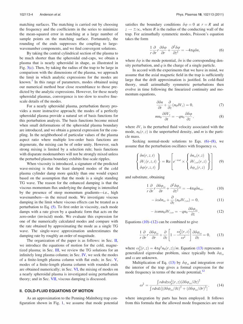
FIG. 3. Three idealized plasma shapes for which the modes of oscillation

are calculated: (a) a cylinder with flat ends, (b) a cylinder with spheroidal

ends, and (c) a spheroid. In each of the three regions separated by the dashed

curves, we express the mode potential as a linear combination of functions

that satisfy the mode equation and boundary conditions in that particular

region. The numerical task is to choose the coefficients in each linear combi-

nation, so that the mode potential and the normal derivative of the electric

displacement match at the boundary surfaces shown here as dashed curves.

102113-3 Degenerate mixing of plasma waves Phys. Plasmas 18, 102113 (2011)

matching surfaces. The matching is carried out by choosing

the frequency and the coefficients in the series to minimize

the mean-squared error in matching at a large number of

sample points on the matching surface. Fortunately, the

rounding of the ends suppresses the coupling to large-

wavenumber components, and we find convergent solutions.

By taking the central cylindrical section of the plasma to

be much shorter than the spheroidal end-caps, we obtain a

plasma that is nearly spheroidal in shape, as illustrated in

Fig. 3(c). Then, by taking the radius of the trap to be large in

comparison with the dimensions of the plasma, we approach

the limit in which analytic expressions for the modes are

known.7 In this range of parameters, modes obtained using

our numerical method bear close resemblance to those pre-

dicted by the analytic expressions. However, for these nearly

spheroidal plasmas, convergence is too slow to resolve fine-

scale details of the modes.

For a nearly spheroidal plasma, perturbation theory pro-

vides a more instructive approach; the modes of a perfectly

spheroidal plasma provide a natural set of basis functions for

this perturbation analysis. The basis functions become mixed

when small deformations of the spheroidal plasma boundary

are introduced, and we obtain a general expression for the cou-

pling. In the neighborhood of particular values of the plasma

aspect ratio where multiple low-order basis functions are

degenerate, the mixing can be of order unity. However, such

strong mixing is limited by a selection rule; basis functions

with disparate modenumbers will not be strongly mixed unless

the perturbed plasma boundary exhibits fine-scale ripples.

When viscosity is introduced, a signature of the predicted

wave-mixing is that the least damped modes of the cold

plasma cylinder damp more quickly than one would expect

based on the assumption that the mode is a single standing

TG wave. The reason for the enhanced damping is that the

viscous momentum flux underlying the damping is intensified

by the presence of steep momentum gradients—i.e., high

wavenumbers—in the mixed mode. We investigate viscous

damping in the limit where viscous effects can be treated as a

perturbation to Eq. (5). To first order in viscosity, each mode

damps with a rate given by a quadratic form that acts on the

zero-order (inviscid) mode. We evaluate this expression for

one of the numerically calculated modes and compare with

the rate obtained by approximating the mode as a single TG

wave. The single-wave approximation underestimates the

damping rate by roughly an order of magnitude.

The organization of the paper is as follows: in Sec. II,

we introduce the equations of motion for the cold, magne-

tized plasma; in Sec. III, we review the TG solutions for an

infinitely long plasma column; in Sec. IV, we seek the modes

of a finite-length plasma column with flat ends; in Sec. V,

modes of a finite-length plasma column with rounded ends

are obtained numerically; in Sec. VI, the mixing of modes on

a nearly spheroidal plasma is investigated using perturbation

theory; and in Sec. VII, viscous damping is discussed.

II. COLD-FLUID EQUATIONS OF MOTION

As an approximation to the Penning-Malmberg trap con-

figuration shown in Fig. 1, we assume that mode potential

satisfies the boundary conditions du ¼ 0 at r ¼ R and at

z! 61, where R is the radius of the conducting wall of the

trap. For azimuthally symmetric modes, Poisson’s equation

takes the form

1

r

@

@rr@du@rþ @

2du@z2

¼ �4pqdn; (6)

where du is the mode potential, dn is the corresponding den-

sity perturbation, and q is the charge of a single particle.

In accord with the experiments that we have in mind, we

assume that the axial magnetic field in the trap is sufficiently

large that the drift approximation is justified. In cold-fluid

theory, small azimuthally symmetric perturbations then

evolve in time following the linearized continuity and mo-

mentum equations,

@dn

@tþ @

@zðn0dVzÞ ¼ 0; (7)

mn0

@dVz

@t¼ �qn0

@du@z

; (8)

where dVz is the perturbed fluid velocity associated with the

mode, n0ðr; zÞ is the unperturbed density, and m is the parti-

cle mass.

Seeking normal-mode solutions to Eqs. (6)–(8), we

assume that the perturbation oscillates with frequency x,

dnðr; z; tÞdVzðr; z; tÞduðr; z; tÞ

8><>:

9>=>; ¼ Re e�ixt �

dnxðr; zÞdVz;xðr; zÞduxðr; zÞ

8><>:

9>=>;

264

375 (9)

and substitute, obtaining

1

r

@

@rr@dux

@rþ @

2dux

@z2¼ �4pqdnx; (10)

� ixdnx þ@

@zðn0dVz;xÞ ¼ 0; (11)

� ixmn0dVz;x ¼ �qn0

@dux

@z: (12)

Equations (10)–(12) can be combined to give

1

r

@

@rr@dux

@rþ @

@z1�

x2pðr; zÞx2

" #@dux

@z¼ 0; (13)

where x2pðr; zÞ ¼ 4pq2n0ðr; zÞ=m: Equation (13) represents a

generalized eigenvalue problem, since typically both dux

and x are unknown.

Multiplication of Eq. (13) by dux and integration over

the interior of the trap gives a formal expression for the

mode frequency in terms of the mode potential,12

x2 ¼Ð

rdrdzx2pðr; zÞð@dux=@zÞ2Ð

rdrdz½ð@dux=@zÞ2 þ ð@dux=@rÞ2�; (14)

where integration by parts has been employed. It follows

from this formula that the allowed mode frequencies are real

102113-4 Anderson et al. Phys. Plasmas 18, 102113 (2011)

and bounded by the plasma frequency; that is, 0 � x2

� max½x2pðr; zÞ� ¼ x2

p:Alternatively, one can derive an integral equation13

for the z-component of the mode electric field, dEz;x

¼ �@dux=@z, by inverting Poisson’s equation with the

Green’s function, Gðr; zjr0; z0Þ, defined by the conditions

1

r

@

@rr@G

@rþ @

2G

@z2¼ dðr � r0Þdðz� z0Þ

r; (15)

Gjr¼R ¼ Gjjz�z0j!1 ¼ 0: (16)

In terms of the Green’s function, Eq. (10) can be recast in

the form

duxðr; zÞ ¼ �4pq

ðr0dr0dz0dnxðr0; z0ÞGðr; zjr0; z0Þ: (17)

Equations (11) and (12) give the perturbed density in terms

of the electric field,

4pqdnx ¼ �@

@z

x2pðr; zÞx2

dEz;x

" #: (18)

Inserting this expression in Eq. (17), integrating by parts,

and taking the partial derivative with respect to z, one obtains

the integral equation

x2dEz;xðr;zÞ¼�ð

r0dr0dz0x2pðr0;z0Þ

@G

@z@z0dEz;xðr0;z0Þ: (19)

Unlike Eq. (13), Eq. (19) constitutes a linear eigenvalue

problem, �x2 being the eigenvalue, and dEz;x, the eigen-

function. Furthermore, the integral operator on the right-

hand-side is self-adjoint with respect to the inner product

ðf1; f2Þ �Ð

rdrdzx2pðr; zÞf1f2; It follows that all mode fre-

quencies are real and that for any two modes with distinct

frequencies x and x0 the axial electric fields are orthogonal

inside the plasma,ðrdrdzx2

pðr; zÞdEz;xðr; zÞdEz;x0 ðr; zÞ ¼ 0 ðx 6¼ x0Þ: (20)

While the integral equation (19) is equivalent to the dif-

ferential equation (13) (with boundary conditions), it should

be emphasized that dEz;x—not dux—is the true eigenfunc-

tion. For a mode that consists of many component waves,

this distinction is important, since it is easy to underestimate

the degree of the mixing when viewing a plot of the mode

potential (see Figs. 5 and 8). For example, a wave with axial

wavenumber kz that appears with amplitude A in the z-com-

ponent of the mode electric field will appear with amplitude

A=kz in the mode potential, since dEz;x ¼ �@dux=@z: In this

sense, large axial wavenumbers are suppressed relative to

smaller wavenumbers in the mode potential. In contrast, the

density gives an exaggerated impression of the mixing; a

wave which appears with amplitude A in the z-component of

the mode electric field will appear with amplitude

ðk2?jk2

z ÞA=kz in the mode density.

III. TRIVELPIECE-GOULD WAVES

Before considering modes of a finite-length plasma cyl-

inder, we present the solutions of Eq. (13) obtained by Triv-

elpiece and Gould for the case of an infinitely long cylinder.9

In this case, Eq. (13) simplifies to

1

r

@

@rr@dux

@rþ 1�

x2pðrÞx2

" #@2dux

@z2¼ 0; (21)

which is separable. Specifically, for any real x, there exist

an infinite number of degenerate solutions of the form

duxðr; zÞ ¼ wTGm ðx; rÞe6ikmz: (22)

Substitution into Eq. (21) yields a differential equation for

the radial dependence, wTGm ðx; rÞ,

1

r

d

drr

dwTGm ðx; rÞ

dr� k2

m 1�x2

pðrÞx2

" #wTG

m ðx; rÞ ¼ 0: (23)

In thermal equilibrium, the radial plasma density profile,

n0ðrÞ, is nearly constant out to some radius and there

abruptly falls off on the scale of the Debye length. Following

Trivelpiece and Gould, we take an unperturbed density pro-

file that is constant out to some radius, a, and zero outside

this radius,

n0ðrÞ ¼ n0Hðr � aÞ; (24)

where H(x) is the Heaviside step function. This choice corre-

sponds to an equilibrium density profile in the limit of zero

temperature. A finite-temperature equilibrium density profile

in place of the approximation (24) would necessitate numeri-

cal solution of Eq. (23), but the qualitative behavior of these

solutions (e.g., oscillatory out to some radius; monotonically

decreasing outside this radius) would be the same.

With the assumption of a step-function density profile,

Eq. (23) becomes a Bessel equation in the domain r < a and

a modified Bessel equation in the domain a < r < R: Mak-

ing use of the boundary condition du ¼ 0 at r ¼ R and

requiring that du be continuous at r ¼ a, one finds solutions

of the form

wTGm ðx;rÞ�

J0

�kmr

ffiffiffiffiffiffiffiffiffiffiffiffiffiffiffiffiffiffiffiffiffix2

p=x2�1

q �J0

�kma

ffiffiffiffiffiffiffiffiffiffiffiffiffiffiffiffiffiffiffiffiffix2

p=x2�1

q � r� a

I0ðkmrÞK0ðkmRÞ� I0ðkmRÞK0ðkmrÞI0ðkmaÞK0ðkmRÞ� I0ðkmRÞK0ðkmaÞ a< r�R:

8>>>>><>>>>>:

(25)

The wavenumber km ¼ kmðxÞ is given by the mth nonnega-

tive solution to the equation

ffiffiffiffiffiffiffiffiffiffiffiffiffiffiffiffiffiffiffiffiffiffix2

p=x2 � 1

q J1

�ka

ffiffiffiffiffiffiffiffiffiffiffiffiffiffiffiffiffiffiffiffiffiffix2

p=x2 � 1

q �J0

�ka

ffiffiffiffiffiffiffiffiffiffiffiffiffiffix2

p=x2

q� 1

�þ I00ðkaÞK0ðkRÞ � I0ðkRÞK00ðkaÞ

I0ðkaÞK0ðkRÞ � I0ðkRÞK0ðkaÞ ¼ 0; (26)

102113-5 Degenerate mixing of plasma waves Phys. Plasmas 18, 102113 (2011)

which comes from the requirement that @du=@r be con-

tinuous at r ¼ a. These are the azimuthally symmetric

Trivelpiece-Gould waves. By defining the transverse wave-

number k?;m � kmðx2p=x

2 � 1Þ1=2, one recovers the disper-

sion equation (1).

In addition to the Trivelpiece-Gould waves, there exists

another class of solutions to Eq. (21) of the form11

duxðr; zÞ ¼ wAmðx; rÞe6jmz: (27)

For these solutions, the radial dependence is given by

wAmðx;rÞ�

I0

�jmr

ffiffiffiffiffiffiffiffiffiffiffiffiffiffiffiffiffiffiffiffiffix2

p=x2�1

q �I0

�jma

ffiffiffiffiffiffiffiffiffiffiffiffiffiffiffiffiffiffiffiffiffix2

p=x2�1

q � r�a

J0ðjmrÞN0ðjmRÞ�J0ðjmRÞN0ðjmrÞJ0ðjmaÞN0ðjmRÞ�J0ðjmRÞN0ðjmaÞ a< r�R;

8>>>>><>>>>>:

(28)

where jm is the mth nonnegative solution to the equation

ffiffiffiffiffiffiffiffiffiffiffiffiffiffiffiffiffiffiffiffiffiffix2

p=x2 � 1

q I1

�ja

ffiffiffiffiffiffiffiffiffiffiffiffiffiffiffiffiffiffiffiffiffiffix2

p=x2 � 1

q �I0

�ja

ffiffiffiffiffiffiffiffiffiffiffiffiffiffiffiffiffiffiffiffiffiffix2

p=x2 � 1

q �þ J00ðjaÞN0ðjRÞ � J0ðjRÞN00ðjaÞ

J0ðjaÞN0ðjRÞ � J0ðjRÞN0ðjaÞ ¼ 0: (29)

We will refer to these solutions as “annular solutions,” since

they are localized in the annular vacuum region a < r < R.

Because the annular solutions become exponentially large as

z! 61, they are typically ignored in the theory of the

infinitely long cylinder; however, we will need these solu-

tions when we solve for modes of a finite-length plasma

cylinder.

The functions wTGm ðx; rÞ and wA

mðx; rÞ are mutually

orthogonal on the interval 0 < r < R with weight function

eðx; rÞ � 1� x2pðrÞ=x2; we choose the normalization so that11

ðR

0

rdreðx; rÞwTGm ðx; rÞwTG

m0 ðx; rÞ ¼ �R2

2dmm0 (30)

and ðR

0

rdreðx; rÞwAmðx; rÞwA

mðx; rÞ ¼ R2

2dmm0 : (31)

The difference in sign ensures that both wTGm ðx; rÞ and

wAmðx; rÞ are real-valued functions, since the function eðx; rÞ

is negative inside the plasma, where the functions wTGm ðx; rÞ

are localized, and positive outside the plasma, where the

functions wAmðx; rÞ are localized. Several of the functions

wTGm ðx; rÞ and wA

mðx; rÞ are plotted in Fig. 4 for R ¼ 1;a ¼ 1=2, and x=xp ¼ 1=10.

IV. MODES OF A PLASMA COLUMN WITH FLAT ENDS

We now search for modes of a finite-length plasma

cylinder. Jennings et al. approached this problem by discre-

tizing equation (13), while Rasband et al. employed a finite-

element method.12,14 Following Prasad and O’Neil,11 we

choose to represent each mode as a linear combination of

the TG and annular solutions discussed in Sec. III. This

approach manifests the mixing of degenerate waves.

In this section, we focus on a well-known model which

takes the unperturbed plasma density to be constant inside a

right-circular cylinder of radius a and length L and zero out-

side this cylinder [Fig. 3(a)],

n0ðr; zÞ ¼ n0Hðr � aÞHðjzj � L=2Þ: (32)

In this case, although the Trivelpiece-Gould and annular sol-

utions are no longer global solutions to Eq. (13), they still

satisfy this equation in the region jzj < L=2. We assume that

the mode potential in this region can be expressed as a linear

combination of these solutions,

duxðr; zÞ ¼X1m¼1

BmwTGm ðx; rÞ sinðkmzÞ

sinðkmL=2Þ

þX1m¼1

CmwAmðx; rÞ sinhðjmzÞ

sinhðjmL=2Þ: (33)

For jzj > L=2, Eq. (13) reduces to Laplace’s equation, and

thus, in this region, the mode potential can be expressed as a

linear combination of vacuum solutions,

duxðr; zÞ ¼ signðzÞX1n¼1

AnJ0ðv0nr=RÞe�v0nðz�L=2Þ=R: (34)

FIG. 4. Several of the functions wTGm ðx; rÞ and wA

mðx; rÞ plotted for the

parameter values x=xp ¼ 0:1, a ¼ 0:5, and R ¼ 1. These functions give the

radial dependence of the Trivelpiece-Gould and annular solutions on an

infinitely long plasma cylinder.

102113-6 Anderson et al. Phys. Plasmas 18, 102113 (2011)

Here, we have assumed that the mode potential is odd in z;

the generalization to even modes is straightforward.

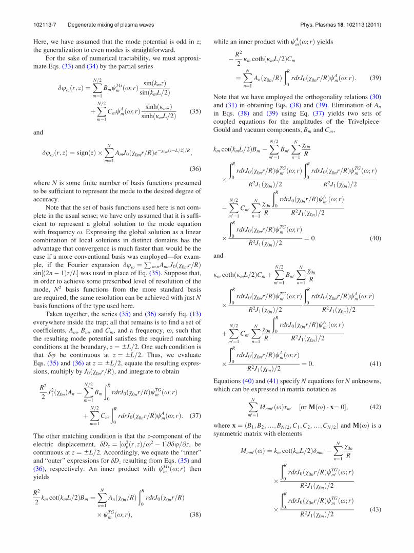
For the sake of numerical tractability, we must approxi-

mate Eqs. (33) and (34) by the partial series

duxðr; zÞ ¼XN=2

m¼1

BmwTGm ðx; rÞ sinðkmzÞ

sinðkmL=2Þ

þXN=2

m¼1

CmwAmðx; rÞ sinhðjmzÞ

sinhðjmL=2Þ (35)

and

duxðr; zÞ ¼ signðzÞ �XN

m¼1

AmJ0ðv0mr=RÞe�v0mðz�L=2Þ=R;

(36)

where N is some finite number of basis functions presumed

to be sufficient to represent the mode to the desired degree of

accuracy.

Note that the set of basis functions used here is not com-

plete in the usual sense; we have only assumed that it is suffi-

cient to represent a global solution to the mode equation

with frequency x. Expressing the global solution as a linear

combination of local solutions in distinct domains has the

advantage that convergence is much faster than would be the

case if a more conventional basis was employed—for exam-

ple, if the Fourier expansion dux ¼P

m;nAmnJ0ðv0mr=RÞsin½ð2n� 1Þz=L� was used in place of Eq. (35). Suppose that,

in order to achieve some prescribed level of resolution of the

mode, N2 basis functions from the more standard basis

are required; the same resolution can be achieved with just Nbasis functions of the type used here.

Taken together, the series (35) and (36) satisfy Eq. (13)

everywhere inside the trap; all that remains is to find a set of

coefficients, Am, Bm, and Cm, and a frequency, x, such that

the resulting mode potential satisfies the required matching

conditions at the boundary, z ¼ 6L=2: One such condition is

that du be continuous at z ¼ 6L=2. Thus, we evaluate

Eqs. (35) and (36) at z ¼ 6L=2, equate the resulting expres-

sions, multiply by J0ðv0nr=RÞ, and integrate to obtain

R2

2J2

1ðv0nÞAn ¼XN=2

m¼1

Bm

ðR

0

rdrJ0ðv0nr=RÞwTGm ðx; rÞ

þXN=2

m¼1

Cm

ðR

0

rdrJ0ðv0nr=RÞwAmðx; rÞ: (37)

The other matching condition is that the z-component of the

electric displacement, dDz ¼ ½x2pðr; zÞ=x2 � 1�@du=@z, be

continuous at z ¼ 6L=2. Accordingly, we equate the “inner”

and “outer” expressions for dDz resulting from Eqs. (35) and

(36), respectively. An inner product with wTGm ðx; rÞ then

yields

R2

2km cotðkmL=2ÞBm ¼

XN

n¼1

Anðv0n=RÞðR

0

rdrJ0ðv0nr=RÞ

� wTGm ðx; rÞ; (38)

while an inner product with wAmðx; rÞ yields

� R2

2jm cothðjmL=2ÞCm

¼XN

n¼1

Anðv0n=RÞðR

0

rdrJ0ðv0nr=RÞwAmðx; rÞ: (39)

Note that we have employed the orthogonality relations (30)

and (31) in obtaining Eqs. (38) and (39). Elimination of An

in Eqs. (38) and (39) using Eq. (37) yields two sets of

coupled equations for the amplitudes of the Trivelpiece-

Gould and vacuum components, Bm and Cm,

km cotðkmL=2ÞBm �XN=2

m0¼1

Bm0XN

n¼1

v0n

R

�

ðR

0

rdrJ0ðv0nr=RÞwTGm0 ðx; rÞ

R2J1ðv0nÞ=2

ðR

0

rdrJ0ðv0nr=RÞwTGm ðx; rÞ

R2J1ðv0nÞ=2

�XN=2

m0¼1

Cm0XN

n¼1

v0n

R

ðR

0

rdrJ0ðv0nr=RÞwAm0 ðx; rÞ

R2J1ðv0nÞ=2

�

ðR

0

rdrJ0ðv0nr=RÞwTGm ðx; rÞ

R2J1ðv0nÞ=2¼ 0: (40)

and

jm cothðjmL=2ÞCm þXN=2

m0¼1

Bm0XN

n¼1

v0n

R

�

ðR

0

rdrJ0ðv0nr=RÞwTGm0 ðx; rÞ

R2J1ðv0nÞ=2

ðR

0

rdrJ0ðv0nr=RÞwAmðx; rÞ

R2J1ðv0nÞ=2

þXN=2

m0¼1

Cm0XN

n¼1

v0n

R

ðR

0

rdrJ0ðv0nr=RÞwAm0 ðx; rÞ

R2J1ðv0nÞ=2

�

ðR

0

rdrJ0ðv0nr=RÞwAmðx; rÞ

R2J1ðv0nÞ=2¼ 0: (41)

Equations (40) and (41) specify N equations for N unknowns,

which can be expressed in matrix notation as

XN

m0¼1

Mmm0 ðxÞxm0 ½or MðxÞ x¼ 0�; (42)

where x ¼ ðB1;B2;…;BN=2;C1;C2;…;CN=2Þ and MðxÞ is a

symmetric matrix with elements

Mmm0 ðxÞ ¼ km cotðkmL=2Þdmm0 �XN

n¼1

v0n

R

�

ðR

0

rdrJ0ðv0nr=RÞwTGm0 ðx; rÞ

R2J1ðv0nÞ=2

�

ðR

0

rdrJ0ðv0nr=RÞwTGm ðx; rÞ

R2J1ðv0nÞ=2(43)

102113-7 Degenerate mixing of plasma waves Phys. Plasmas 18, 102113 (2011)

for m � N=2 and m0 � N=2,

Mmm0 ðxÞ ¼ jm cothðjmL=2Þdmm0 �XN

n¼1

v0n

R

�

ðR

0

rdrJ0ðv0nr=RÞwAm0 ðx; rÞ

R2J1ðv0nÞ=2

�

ðR

0

rdrJ0ðv0nr=RÞwAmðx; rÞ

R2J1ðv0nÞ=2(44)

for N=2 < m � N and N=2 < m0 � N, and

Mmm0 ðxÞ ¼ �XN

n¼1

v0n

R

ðR

0

rdrJ0ðv0nr=RÞwAm0 ðx; rÞ

R2J1ðv0nÞ=2

�

ðR

0

rdrJ0ðv0nr=RÞwTGm ðx; rÞ

R2J1ðv0nÞ=2(45)

for m � N=2 and N=2 < m0 � N. Equation (42) constitutes a

generalized eigenvalue problem; each matrix element

depends on the unknown mode frequency, x through the

functions wTGm ðx; rÞ and wA

mðx; rÞ and the wavenumbers

km ¼ kmðxÞ and jm ¼ jmðxÞ.

A. Analytic solution for a = R

In order to better understand the matrix equation (42), it

is instructive to consider the simple case in which the plasma

extends to the trap wall—that is, a ¼ R. In this case, there

are no annular solutions, so the matrix M is given entirely by

Eq. (43). Furthermore, the TG solutions have the same radial

dependence as the vacuum solutions,

wTGm ðx; rÞ ¼ k2

mðxÞðv0m=RÞ2

J0ðv0mr=RÞJ1ðv0mÞ

(46)

[the normalization follows from Eq. (30)]. Consequently, the

second term on the right-hand side of Eq. (43) is zero unless

m ¼ m0, implying that a given TG wave reflects entirely

back into itself at z ¼ 6L=2. In other words, the matrix M is

diagonal, and Eq. (46) takes the simple form

½km cotðkmL=2Þ � k2mR=v0m�Bm ¼ 0: (47)

Thus, when the plasma extends to the trap wall, the modes

are just standing TG waves with radial dependence given by

Eq. (46) and axial wavenumber quantized according to the

condition that the diagonal matrix element equal zero,

cotðkmL=2Þ � kmR=v0m ¼ 0: (48)

For a long plasma, it follows that for radial modenumber m,

the allowed axial wavenumbers are given by kmn

¼ ð2n� 1Þp=L� dkmn; where n is an integer and dkmn is a

correction of order R=L2. Inserting this expression in

Eq. (48) and expanding the cotangent term, one finds that to

first order in R=L2, dkmn ffi ð2n� 1Þ2pR=ðv0mL2Þ.

B. Numerical solution for a < R

When the plasma does not extend to the trap wall, the

radialdependence of the TG waves no longer matches that of

the vacuum solutions. Consequently, at z ¼ 6L=2, an inci-

dent TG wave reflects partially back into itself and partially

into other TG waves. It follows that each mode must be a

mixture of multiple component waves. From a cursory analy-

sis of the matrix M, one can guess which waves should

appear prominently in the admixture for a mode with fre-

quency x. According to the normalization condition (30),

the second term on the right-hand side of Eq. (43)—and thus

any off-diagonal matrix element—is of order R=L2 or

smaller.11 In contrast, the first term on the right-hand side of

Eq. (43), which appears only on the diagonal of the matrix,

can be any size, diverging as kmðxÞL=2 approaches any mul-

tiple of p, and vanishing as kmðxÞL=2 approaches any odd

multiple of p=2. If the wavenumber kmðxÞ is such that

km cotðkmL=2Þj � R=L2, the mth diagonal element will be

large, and one can see that the amplitude of the mth wave

must then be small in order for Eq. (42) to be satisfied. Con-

versely, the amplitude of the mth wave may be large only if

the mth diagonal element is small compared to R=L2; as in

the previous example, this occurs for wavenumbers kmðxÞ¼ ð2n� 1Þp=L� dkmðxÞ, where n is an integer and dkmðxÞis a correction of order R=L2. For a given mode frequency,

there can be many such waves, and these waves will give the

dominant contribution to the admixture for that mode.

The heuristic argument outlined in the preceding para-

graph is a revised version of an argument introduced by Pra-

sad and O’Neil.11 These authors derived a generalized

version of Eq. (10) for a mode with azimuthal dependence

and carried out a perturbative solution based on the small-

ness of the off-diagonal matrix elements. However, a tacit

assumption underlying the perturbation theory is that only

one of the diagonal elements of the matrix is small compared

to the off-diagonal elements in its row, and this assumption

is unjustified.

We proceed by evaluating the matrix MðxÞ on a grid in

x-space and calculating the determinant at each point on this

grid. We search for values of x for which Det½MðxÞ� ¼ 0, at

these values, the null-vector, x, gives a solution to Eq. (42).

As expected, the contribution to each solution is greatest

from wavenumbers kmðxÞ ffi ð2n� 1Þp=L. However, as the

number of basis functions, N, is increased, increasingly

short-wavelength waves enter the admixture for each solu-

tion with significant amplitude, and this trend continues to

the limit of our computational capability. The lack of conver-

gence should not be surprising. The off-diagonal matrix ele-

ments fall off only as m�1 and are non-negligible even for

large m; thus, for arbitrarily large m, the mth diagonal matrix

element can still be smaller than the off-diagonal elements in

the mth row, provided that the wavenumber km is close

enough to ð2n� 1Þp=L, where n is an integer.

An exemplary solution is plotted in Fig. 5—with various

numbers of basis functions retained—as an illustration of the

appearance of increasingly large wavenumbers in each solu-

tion. In Fig. 5(a), only four TG waves are retained, and the

dominant term in the admixture comes from the first TG

102113-8 Anderson et al. Phys. Plasmas 18, 102113 (2011)

wave, which has wavenumber k1ðxÞ ffi 3p=L� 6:94ðR=L2Þ,where x is the frequency of the solution. In Fig. 5(b), eight

waves are retained, and now the seventh wave, which has

wavelength k7ðxÞ ffi 39p=L� 2:45ðR=L2Þ, enters the admix-

ture with amplitude comparable to that of the first wave.

With more waves retained, the solution incurs significant

contributions from even shorter wavelengths.

V. MODES OF A PLASMA COLUMNWITH SPHEROIDAL END-SHAPE

There is a reason to suspect that the appearance of

increasingly short wavelengths in each of the solutions

obtained in Sec. IV stems from the crude approximation of

the plasma shape as a cylinder with perfectly flat ends and

hence sharp edges. The mode structure is determined by the

coupling between TG waves reflecting at the ends of the

plasma cylinder, and this coupling must be affected by the

end-shape. In this section, we generalize the method of Sec.

IV and look for modes of a plasma cylinder with spheroidal

end-shape. In this case, the plasma boundary is given by

r ¼ a for jzj < L=2 and by ½ðz� L=2Þ=ðDL0=2Þ�2þðr=aÞ2 ¼ 1 for jzj > L=2, where DL0 is the combined

length of the two spheroidal end caps. Note that this plasma

boundary has no sharp edges. For long cylindrical plasmas

satisfying the ordering L� R � a; the curvature of the ends

of the plasma cylinder in equilibrium is typically of order

1=a; so we will consider end-shapes with DL0 of order a.3

Following the procedure of Sec. IV, we divide the space

inside the trap into regions with distinct solution sets, as

depicted in Fig. 3(b). The surface that separates these regions

is given by z ¼ ½Lþ DLðrÞ�=2, where

DLðrÞ2¼ ðDL0=2Þ

ffiffiffiffiffiffiffiffiffiffiffiffiffiffiffiffiffiffiffiffiffi1� ðr=aÞ2

qr < a

0 a < r < R

((49)

is the deviation from the flat matching surface taken in Sec.

VI. We express the mode potential as the series (35) and (36)

in the appropriate domains. Again, the matching conditions

on du and dD ¼ ½x2pðr; zÞ=x2 � 1�ð@du=@zÞz� ð@du=@rÞr

yield coupled equations for the coefficients Bn and Cn. The

continuity of du gives

XN

n¼1

AnJ0ðv0nr=RÞe�v0nDLðrÞð2RÞ

¼XN=2

m¼1

BmwTGm ðx; rÞ sinfkmðxÞ½Lþ DLðrÞ�=2g

sinfkmðxÞL=2g

þXN=2

m¼1

CmwAmðx; rÞ sinhfjmðxÞ½Lþ DLðrÞ�=2g

sinhfjmðxÞL=2g ; (50)

FIG. 5. (Color online) The axial electric field, dEz;x, and potential, dux, corresponding to a solution of the matrix equation (42) obtained by retaining 8 terms

(a) and 16 terms (b) in the series (35) and (36). The plasma has length L ¼ 14:0 and radius a ¼ 0:5, and the trap has radius R ¼ 1:0. As the number of basis

functions is increased, the solution involves increasingly large wavenumbers.

102113-9 Degenerate mixing of plasma waves Phys. Plasmas 18, 102113 (2011)

while the continuity of dD n gives

XN

n¼1

Anðv0n=RÞe�v0nDLðrÞ=ð2RÞ½nzðrÞJ0ðv0nr=RÞþnrðrÞJ1ðv0nr=RÞ�

¼�XN=2

m¼1

Bm

�nrðrÞ

dwTGm ðx;rÞ

dr

sinfkmðxÞ½LþDLðrÞ�=2gsinfkmðxÞL=2g

þnzðrÞeðx;rÞkmðxÞwTGm ðx;rÞcosfkmðxÞ½LþDLðrÞ�=2g

sinfkmðxÞL=2g

�

�XN=2

m¼1

Cm

�nrðrÞ

dwAmðx;rÞdr

sinhfjmðxÞ½LþDLðrÞ�=2gsinhfjmðxÞL=2g

þnzðrÞeðx;rÞjmðxÞwAmðx;rÞcoshfjmðxÞ½LþDLðrÞ�=2g

sinhfjmðxÞL=2g

�;

(51)

where nrðrÞ and nzðrÞ are the radial and axial components of

the unit vector n that is normal to the matching surface.

The analysis of Sec. IV relies on the orthogonality prop-

erties of the Bessel functions and the functions wTGm ðx; rÞ

and wAmðx; rÞ, however, this approach fails here because the

curvature of the plasma boundary introduces additional r-de-

pendence. Instead, we discretize the radial coordinate, taking

P points, {r1, r2,…, rP}, and evaluate Eqs. (50) and (51) on

this grid, obtaining two sets of coupled equations,

XN

n¼1

AnJ0ðv0nrp=RÞe�v0nDLðrpÞ=ð2RÞ

¼XN=2

m¼1

BmwTGm ðx; rpÞ

sinfkmðxÞ½Lþ DLðrpÞ�=2gsinfkmðxÞL=2g

þXN=2

m¼1

CmwAmðx; rpÞ

sinhfjmðxÞ½Lþ DLðrpÞ�=2gsinhfjmðxÞL=2g (52)

and

XN

n¼1

Anðv0n=RÞe�v0nDLðrÞ=ð2RÞ

� ½nzðrpÞJ0ðv0nrp=RÞ þ nrðrpÞJ1ðv0nrp=RÞ�

¼ �XN=2

m¼1

Bm

�nrðrpÞ

dwTGm ðx; rÞ

dr

����r¼rp

� sinfkmðxÞ½Lþ DLðrpÞ�=2gsinfkmðxÞL=2g þ nzðrpÞeðx; rpÞkmðxÞ

� wTGm ðx; rpÞ

cosfkmðxÞ½Lþ DLðrpÞ�=2gsinfkmðxÞL=2g

�

�XN=2

m¼1

Cm

�nrðrpÞ

dwAmðx; rÞdr

����r¼rp

� sinhfjmðxÞ½Lþ DLðrpÞ�=2gsinhfjmðxÞL=2g þ nzðrpÞeðx; rpÞjmðxÞ

� wAmðx; rpÞ

coshfjmðxÞ½Lþ DLðrpÞ�=2gsinhfjmðxÞL=2g

�: (53)

Equations (52) and (53) comprise a system of 2P equations

for 2N unknowns and can be expressed as a single matrix

equation,

X2N

n¼1

M0pnðxÞx0n ¼ 0 ½or M0ðxÞ x0 ¼ 0�; (54)

where x0 ¼ ðA1;A2;…;AN;B1;B2;…;BN=2;C1;C2;…;CN=2Þand M0ðxÞ is a 2P� 2N matrix; the primes are a reminder

that the matrix M0 and the vector x0 are distinct from M and

x as defined in Sec. IV.

In order for every basis function to be well-resolved on

the radial grid, we take P� N, and thus, Eq. (54) becomes

an over-determined system of equations that cannot be satis-

fied exactly. Thus, we seek a nonzero vector x0 and fre-

quency x that together minimize the mean squared

mismatch at the boundary, Dðx; x0Þ, defined as

Dðx; x0Þ � 1

P½M0ðxÞ x0�2: (55)

We exclude the trivial solution, x0 ¼ 0, by imposing a nor-

malization constraint. We observe that a variety of different

normalization constraints lead to the same solutions. A sim-

ple choice is the following:

SðxÞ x0½ �2 ¼ 1; (56)

where

Snn0 ðxÞ ¼knðxÞdnn0

sin kn xð ÞL=2½ � ; (57)

for n � N=2 and Snn0 ¼ 0 otherwise. This constraint simply

requires that the squared amplitudes of all Trivelpiece-Gould

components making up the mode electric field sum to one.

For fixed x, the minima of Dðx; x0Þ under this normal-

ization constraint are given by the condition

d M0ðxÞ x0½ �2 � k SðxÞ x0½ �f 2 � 1g� �

¼ 0; (58)

where k is a Lagrange multiplier and the variation is taken

with respect to x0. Carrying out the variation yields

M0TðxÞ M0ðxÞ x0 ¼ kSTðxÞ SðxÞ x0; (59)

where the superscript T denotes the transpose. In other

words, for fixed x the local minima of Dðx; x0Þ are given by

the “generalized eigenvectors” of the matrix M0TðxÞ M0ðxÞwith respect to the matrix STðxÞ SðxÞ. The global mini-

mum (on the surface of constraint) is given by the eigenvec-

tor with the smallest eigenvalue; all eigenvalues are positive

since both M0TðxÞ M0ðxÞ and STðxÞ SðxÞ are positive-

definite.

To find a mode frequency, we therefore evaluate the

matrices M0TðxÞ M0ðxÞ and STðxÞ SðxÞ on a grid in xand determine the smallest eigenvalue, kminðxÞ, at each grid

point. For N � 1, the function kminðxÞ typically has many

local minima. As N and P are increased, some of these min-

ima approach zero (as does the corresponding mismatch),

and the value of x, where such a minimum occurs, gives the

frequency of a mode. The mode potential is given by the

eigenvector, x0, corresponding to kminðxÞ at the mode fre-

quency. The procedure is illustrated in Fig. 6.

102113-10 Anderson et al. Phys. Plasmas 18, 102113 (2011)

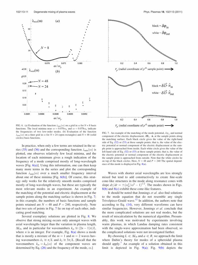
In practice, when only a few terms are retained in the se-

ries (35) and (36) and the corresponding function kminðxÞ is

plotted, one observes relatively few local minima, and the

location of each minimum gives a rough indication of the

frequency of a mode comprised mostly of long-wavelength

waves [Fig. 6(a)]. Using this information, one can then keep

many more terms in the series and plot the corresponding

function kminðxÞ over a much smaller frequency interval

about one of these minima [Fig. 6(b)]. Of course, this strat-

egy only works for the relatively smooth modes comprised

mostly of long-wavelength waves, but these are typically the

most relevant modes in an experiment. An example of

the matching of the potential and electric displacement at the

sample points along the matching surface is shown in Fig. 7;

in this example, the numbers of basis functions and sample

points retained are N ¼ 48 and P ¼ 240, respectively. Note

that two sets of points in Fig. 7 lie on top of each other, indi-

cating good matching.

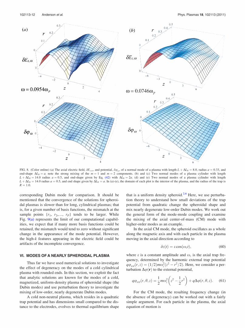
Several exemplary solutions are plotted in Fig. 8. We

observe that strong mixing occurs only amongst waves with

axial wavelengths larger than the variation in plasma length,

DL0, and in particular for wavenumbers km ffi ð2n� 1Þp=L;where n is an integer. For example, Fig. 8(a) shows a mode

that is mostly a mixture of the m ¼ 1 and m ¼ 2 waves hav-

ing wavenumbers k1 ffi p=L and k2 ffi 3p=L. [Recall that the

wavenumbers km ¼ kmðxÞ of the component waves are

determined by Eq. (26) and the frequency of the mode, x.]

Waves with shorter axial wavelengths are less strongly

mixed but tend to add constructively to create fine-scale

cone-like structures in the mode along resonance cones with

slope dz=dr ¼ 6ðx2p=x

2 � 1Þ1=2. The modes shown in Figs.

8(b) and 8(c) exhibit these cone-like features.

It should be noted that Jennings et al. also find solutions

to the mode equation that do not resemble any single

Trivelpiece-Gould wave.12 In addition, the authors note that

according to Eq. (14), very different waveforms can have

similar frequencies. However, Jennings et al. conclude that

the more complicated solutions are not real modes, but the

result of miscalculation by the numerical algorithm. Presum-

ably, this work was motivated by experiments involving

warm plasmas, in which Landau damping rates consistent

with the single-wave approximation had been observed, so

the complicated solutions were not investigated further.

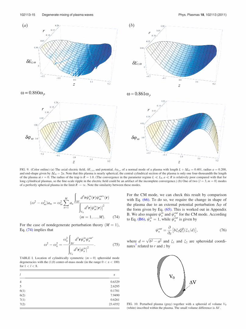
By choosing L� DL0 and a� R, we approach the limit

where Dubin’s theory for modes of a spheroidal plasma

should apply.7 An example of a solution obtained in this

limit is depicted in Fig. 9(a); Fig. 9(b) depicts the

FIG. 6. (a) Evaluation of the function kminðxÞ on a grid in x for N = 8 basis

functions. The local minima near x ¼ 0:070xp and x ¼ 0:078xp indicate

the frequencies of two low-order modes. (b) Evaluation of the function

kminðxÞ on a finer grid in x for N = 24 (open rectangles) and N = 48 (solid

circles) basis functions.

FIG. 7. An example of the matching of the mode potential, dux and normal

component of the electric displacement, dDx n, at the sample points along

the matching surface. Each black circle gives the value of the right-hand

side of Eq. (52) or (53) at these sample points; that is, the value of the elec-

tric potential or normal component of the electric displacement as the sam-

ple point is approached from inside. Each white circle gives the value of the

left-hand side of Eq. (52) or (53) at these sample points; that is, the value of

the electric potential or normal component of the electric displacement as

the sample point is approached from outside. Note that the white circles lie

on top of the black circles. Here, N ¼ 48 and P ¼ 240 The spatial depend-

ence of this mode is displayed in Fig. 8(a).

102113-11 Degenerate mixing of plasma waves Phys. Plasmas 18, 102113 (2011)

corresponding Dubin mode for comparison. It should be

mentioned that the convergence of the solutions for spheroi-

dal plasmas is slower than for long, cylindrical plasmas; that

is, for a given number of basis functions, the mismatch at the

sample points {r1, r2,…, rP} tends to be larger. While

Fig. 9(a) represents the limit of our computational capabil-

ities, we expect that if many more basis functions could be

retained, the mismatch would tend to zero without significant

change in the appearance of the mode potential. However,

the high-k features appearing in the electric field could be

artifacts of the incomplete convergence.

VI. MODES OF A NEARLY SPHEROIDAL PLASMA

Thus far we have used numerical solutions to investigate

the effect of degeneracy on the modes of a cold cylindrical

plasma with rounded ends. In this section, we exploit the fact

that analytic solutions are known for the modes of a cold,

magnetized, uniform-density plasma of spheroidal shape (the

Dubin modes) and use perturbation theory to investigate the

mixing of low-order, nearly degenerate Dubin modes.

A cold non-neutral plasma, which resides in a quadratic

trap potential and has dimensions small compared to the dis-

tance to the electrodes, evolves to thermal equilibrium shape

that is a uniform density spheroid.2,6 Here, we use perturba-

tion theory to understand how small deviations of the trap

potential from quadratic change the spheroidal shape and

mix nearly degenerate low-order Dubin modes. We work out

the general form of the mode-mode coupling and examine

the mixing of the axial center-of-mass (CM) mode with

higher-order modes as an example.

In the axial CM mode, the spheroid oscillates as a whole

along the magnetic axis and with each particle in the plasma

moving in the axial direction according to

dzðtÞ ¼ e cosðxztÞ; (60)

where e is a constant amplitude and xz is the axial trap fre-

quency, determined by the harmonic external trap potential

quextðr; zÞ ¼ ð1=2Þmx2z ðz2 � r2=2Þ. Here, we consider a per-

turbation DuðrÞ to the external potential,

quextðr; h; zÞ ¼1

2mx2

z z2 � 1

2r2

� þ qDuðr; h; zÞ: (61)

For the CM mode, the resulting frequency change (in

the absence of degeneracy) can be worked out with a fairly

simple argument. For each particle in the plasma, the axial

equation of motion is

FIG. 8. (Color online) (a) The axial electric field, dEz;x, and potential, dux, of a normal mode of a plasma with length Lþ DL0 ¼ 8:0, radius a ¼ 0:33, and

end-shape DL0 ¼ a; note the strong mixing of the m ¼ 1 and m ¼ 2 components. (b) and (c) Two normal modes of a plasma cylinder with length

Lþ DL0 ¼ 14:0 radius a ¼ 0:5, and end-shape given by Eq. (42) with DL0 ¼ 2a. (d) and (e) Two normal modes of a plasma cylinder with length

Lþ DL0 ¼ 14:0 radius a ¼ 0:5, and end shape given by DL0 ¼ a. In (a)-(e), the domain of each plot is the interior of the plasma, and the radius of the trap is

R ¼ 1:0.

102113-12 Anderson et al. Phys. Plasmas 18, 102113 (2011)

d2zi

dt2¼ �x2

z zi þXj 6¼i

4pq2

m

@Gðri;rjÞ@zi

� q

m

@DuðriÞ@zi

; (62)

where G is the Green’s function satisfying r2G ¼ dðri � rjÞ.Assuming that G has axial translational symmetry, so that it

depends on zi and zj only through the combination zi � zj, we

sum over the N particles to obtain expressions involving the

center-of-mass position, Z,

d2Z

dt2¼ �x2

z Z � q

Nm

XN

i¼1

@DuðriÞ@zi

: (63)

If we now assume that the mode in question causes positions

to vary according to ri ¼ ri0 þ e cosðxtÞz; we can use this

expression in Eq. (63) to obtain

x2 ¼ x2z þ

q

Nm

XN

i¼1

@2Duðri0Þ@2zi0

: (64)

Furthermore, since Du is already small, we can neglect the

shape change of the equilibrium and sum over equilibrium

positions in a spheroid. For example, if

qDu ¼ 1

2mx2

z

X1n¼3

bn

rn

Rn�2Pnðcos hÞ (65)

(a spherical harmonic expansion, with R the distance to the

trap electrodes), then Eq. (64) implies

x2 ¼ x2z 1þ 6

5b4

ðb2 � a2ÞR2

þ 9

7b6

ðb2 � a2Þ2

R4þ

" #; (66)

where 2a and 2b are, respectively, the diameter and length of

the plasma spheroid.

This simple result provides a useful check for the follow-

ing more general results. However, in particular, it neglects

degeneracies between the CM mode and other modes. There

are many such degenerate modes, each occurring when the

plasma spheroid takes on a particular shape. A list of some of

these modes is provided in Table I.15 The mode numbers land m refer to the spheroidal harmonic of the given mode

potential,7 and the parameter a � b=a gives the plasma shape

for which degeneracy with the CM mode occurs.

We now turn to the affect of perturbations on the mode

eigenfunction (which must be determined using the above

approach), including the effect of degeneracies, for general

spheroidal normal modes. To do so, we employ the integral

operator formalism introduced in Sec. II [Eq. (19)], where

the normal modes of the axial electric field dEz;xðrÞ obey the

eigenvalue equation

x2dEz;xðrÞ ¼ �ð

d3r0x2pðr0Þ

@Gðr; r0Þ@z@z0

dEz;xðr0Þ: (67)

As discussed previously, the integral operator appearing on

the right-hand-side is Hermitian with respect to the inner

product ðf1; f2Þ �Ð

d3rx2pðrÞf1f2; so that its eigenfunctions

FIG. 8. (Continued)

102113-13 Degenerate mixing of plasma waves Phys. Plasmas 18, 102113 (2011)

form a complete orthogonal basis with respect to this inner

product. However, as this is an integral operator, these eigen-

functions are not necessarily continuous functions. In fact,

for a cold plasma with a sharp boundary, dEz;xðrÞ is discon-

tinuous across this boundary. Since the perturbed external

potential changes the shape of this boundary, the following

perturbation theory is somewhat novel in form.

In the cold-fluid limit considered here, the perturbed

potential DuðrÞ causes a shape change to the plasma volume,

V as shown in Fig. 10. The volume integral in Eq. (67) must

be carried out over this volume. In order to apply perturba-

tion theory, we inscribe a spheroid with volume V0 inside V(see Fig. 10). The volume difference DV ¼ V � V0 is

assumed to be small. We then break the integral in Eq. (67)

into integrals over V0 and over DV,

x2dEz;xðrÞ ¼ �ð

V0

d3r0x2p

@Gðr; r0Þ@z@z0

dEz;xðr0Þ

�ð

V0

d3r0x2p

@Gðr; r0Þ@z@z0

dEz;xðr0Þ: (68)

We treat the second integral as a small perturbation. To do

so, we expand dEz;xðrÞ in the eigenfunctions of the first inte-

gral operator for the spheroid V0, with the following proviso.

As previously noted, the eigenfunctions have distinct forms

inside and outside the spheroid, which we refer to, respec-

tively, as winn ðrÞ and wout

n ðrÞ (where n ¼ 1;…;1). We

choose to represent dEz;xðrÞ only in terms of the inner eigen-

functions winn ðrÞ, extending their functional forms beyond V0

into DV. These eigenfunctions have the form eimhf ðr; zÞ,where f is a finite polynomial in r and z; we assume (without

proof) that such polynomials form a complete set for pertur-

bations in the region DV. Thus, we write

dEz;xðrÞ ¼XM

n¼1

anwinn þ

X1m¼Mþ1

enwinn ; (69)

where the coefficients an are of order unity and enj j � 1. For

M ¼ 1; we will obtain results for nondegenerate perturbation

theory, and for M > 1 we will obtain results where M modes

are nearly degenerate.

Substituting Eq. (69) into Eq. (68) and dropping small

terms yields

x2XM

n¼1

anwinn þ

X1n¼Mþ1

enwinn

!

¼XM

n¼1

x2nanw

inn þ

X1n¼Mþ1

x2nenw

inn

� x2p

XM

n¼1

an

ðDV

d3r0@2G

@z@z0win

n ðr0Þ; (70)

where the spheroidal mode frequencies xn are eigenvalues

obtained from the equation

x2nwnðrÞ ¼ �x2

p

ðV0

d3r0@G

@z@z0wnðr0Þ: (71)

Note that solutions of this integral equation yield winn ðrÞ for

r 2 V0 and woutn ðrÞ for r 62 V0. If we now take an inner prod-

uct of Eq. (70) with respect to the M winn functions over

volume V0 and use their orthogonality, we obtain M homoge-

neous equations for the coefficients a1;…; aM:

x2�x2m

�am¼�x2

p

XM

n¼1

an

ðV0

d3rwin�m ðrÞ

ðDV

d3r0@G

@z@z0win

mðr0ÞðV0

d3rjwinmðrÞj

2

ðm¼1;…;MÞ: (72)

Symmetry of G with respect to interchange of r and r0 allows

us to write

x2p

ðV0

d3rwin�m ðrÞ

ðDV

d3r0@G

@z@z0win

mðr0Þ

¼ x2p

ðDV

d3rwinm rð Þ

ðV0

d3r0@G

@z@z0win�

m ðr0Þ

¼ �x2m

ðDV

d3rwinm rð Þwout�

m rð Þ; (73)

where in the last step we use Eq. (71) and note that the

region DV is outside V0 so that the result of the integration

over r0 is wout�m ; the outer spheroidal eigenmode. Thus,

Eq. (72) becomes

FIG. 8. (Continued)

102113-14 Anderson et al. Phys. Plasmas 18, 102113 (2011)

ðx2 � x2mÞam ¼ x2

m

XM

n¼1

an

ðDV

d3rwinn ðrÞwout�

m ðrÞðV0

d3r winmðrÞ

�� ��2ðm ¼ 1;…;MÞ: (74)

For the case of nondegenerate perturbation theory ðM ¼ 1Þ,Eq. (74) implies that

x2 � x2n ¼

x2n

ðDV

d3rwinn wout�

nðV0

d3r winn

�� ��2 : (75)

For the CM mode, we can check this result by comparison

with Eq. (66). To do so, we require the change in shape of

the plasma due to an external potential perturbation Du of

the form given by Eq. (65). This is worked out in Appendix

B. We also require winn and wout

n for the CM mode. According

to Eq. (B6), winn ¼ 1, while wout

n is given by

woutn ¼

@

@Zbn2Q0

1ðn1=dÞ�

; (76)

where d ¼ffiffiffiffiffiffiffiffiffiffiffiffiffiffiffib2 � a2p

and n1 and n2 are spheroidal coordi-

nates7 related to r and z by

FIG. 9. (Color online) (a) The axial electric field, dEz;x, and potential, dux, of a normal mode of a plasma with length Lþ DL0 ¼ 0:401, radius a ¼ 0:200,

and end-shape given by DL0 ¼ 2a. Note that this plasma is nearly spherical; the central cylindrical section of the plasma is only one four-thousandth the length

of the plasma at r ¼ 0. The radius of the trap is R ¼ 1:0. (The convergence in the parameter regime L� L0; a� R is relatively poor compared with that for

long cylindrical plasmas, so the fine-scale ripple in the electric field could be an artifact of the incomplete convergence.) (b) One of two ðl ¼ 3;m ¼ 0Þ modes

of a perfectly spherical plasma in the limit R!1. Note the similarity between these modes.

TABLE I. Location of cylindrically symmetric ðm ¼ 0Þ spheroidal mode

degeneracies with the (1,0) center-of-mass mode (in the range 0 < a < 100)

for 1 < l < 8.

l a

4 0.6329

5 2.6295

6(1) 0.1781

6(2) 7.9490

7(1) 0.6261

7(2) 23.4352 FIG. 10. Perturbed plasma (gray) together with a spheroid of volume V0

(white) inscribed within the plasma. The small volume difference is DV.

102113-15 Degenerate mixing of plasma waves Phys. Plasmas 18, 102113 (2011)

z ¼ n1n2; r2 ¼ ðn21 � d2Þð1� n2

2Þ; (77)

and Qm1 ðxÞ is an associated Legendre function with branch

cuts chosen, so that Qm1 ðxÞ ! 0 as x!1. When these

results are applied to Eq. (75), we do obtain Eq. (66).

The first order corrections to the eigenfunction are also

determined by Eq. (70). Taking an inner product with respect

to winn , where m ¼ M þ 1;…;1 yields

ðx2 � x2mÞem ¼

XMn¼1

an

x2m

ðDV

d3rwinn wout�

mðV0

d3r winm

�� ��2ðm ¼ M þ 1;…;1Þ: (78)

Thus, em is small provided that DV is small andðx2 � x2

mÞ=x2m is not small. Of course, this latter condition

breaks down at mode degeneracies, which is why, in such

cases, any degenerate modes must be included in the set of

M modes that have order unity contributions to dEz;x. For

degeneracy, the analysis is somewhat simplified by employ-

ing orthonormal eigenmodes such thatðV0

d3r win�� ��2 ¼ 1: (79)

Then, for the case of a single degeneracy ðM ¼ 2Þ, Eq. (78)

implies that

ðx2 � x21 � V11Þðx2 � x2

2 � V22Þ ¼ V12V21; (80)

where

Vij ¼ x2i

ðDV

d3rwinj wout�

i : (81)

Using Eq. (A16), Vij can be written as

Vij ¼ x2i

2pd

1� a2

Xn

Q01ðb=dÞ

Q0nðb=dÞAn

�ð1

�1

dn2Pnðn2Þwinj ðn1 ¼ b; n2Þwout�

i ðn1 ¼ b; n2Þ;

(82)

where the coefficients An are given by Eqs. (A4)–(A10). At

degeneracies, we find that V12 ¼ V�21 (although away from

degeneracy this is not true), so that Eq. (80) predicts real

mode frequencies. Note that since Vij is small, the right-

hand-side of Eq. (80) can be neglected, except near the

degeneracy, where the equation predicts an avoided crossing

since V12V21 > 0. An example is shown for the CM mode in

Fig. 11. According to Table I, the CM mode is degenerate

with a ðl;mÞ ¼ ð4; 0Þ mode when the shape

a ¼ b=a ¼ 0:6329…. Evaluation of Vij, where i; j ¼ 1; 2,

mode 1 being the CM mode and mode 2 the (4,0) mode,

using Duðr; zÞ given by Eq. (65), implies at a ¼ 0:6329,

V11 ¼x2

z a2

R2�0:7193b4 þ 0:4620b6

a2

R2þ

� ; (83)

V22 ¼x2

z a2

R2�1:194b4 þ 0:6685b6

a2

R2þ

� ; (84)

V12 ¼ V21 ¼x2

z a3

R3�0:9674b5 þ 1:107b7

a2

R2þ

� : (85)

The resulting frequencies are plotted in Fig. 11 for a near

0.6329, assuming that only b5 is nonzero. The form of the

(1,0) eigenfunction is strongly modified near the degeneracy.

According to Eq. (78), at the center of the avoided crossing,

the mode dEz becomes an equal mixture of the (1,0) and

(4,0) modes, as shown in Fig. 12. Viscous damping of the

FIG. 11. (Color online) Avoided crossing between CM mode and (4,0)

mode taking b5 ¼ x2z=100 and bn ¼ 0 for n 6¼ 5.

FIG. 12. (Color online) Equal admixture of CM mode and (4,0) mode due

to degeneracy where a ¼ 0:633.

102113-16 Anderson et al. Phys. Plasmas 18, 102113 (2011)

CM mode would display a strong peak around the degener-

acy due to this mixing.

However, there are many other degeneracies with the CM

mode and the (4,0) mode over the range of a plotted in the fig-

ure. Some of these degeneracies with the CM mode are shown

by arrows on the plot. In principle, they would also create

avoided crossings, greatly complicating the plot. Since there

are a countably infinite number of modes, avoided crossings

must occur on a dense set of a values, which could obviate the

predictive value of our perturbative approach. However, most

of these degeneracies are with modes that have highly dispar-

ate spatial scales compared to the low-order CM mode. One

can show that if the perturbed value DV has a smooth shape,

then Vij ! 0 as the spatial scales of modes i and j become

more disparate. Specifically, for a perturbation by a cylindri-

cally symmetric potential Du given by Eq. (65), if wi is a (l,0)

mode and wj is a ð�l; 0Þ mode, then the only bn terms in the

potential that contribute to Vij are those with

n > l� �lþ 1; (86)

and at degeneracy where Vij ¼ Vji,

n > l� �l�� ��þ 1: (87)

Thus, if l� �l�� ��� 1, only very high-order multipoles Du

contribute to Vij In general, Eqs. (A11) and (87) imply that,

to lowest order in bn and a=R,

Vij /a

R

� �jl��ljbjl��ljþ2 ; (88)

for l� �l�� �� 1. For small bn and=or a=R and large l� �l

�� ��,this implies that the avoided crossings are extremely narrow

and can be neglected.

VII. VISCOUS DAMPING

In the low-temperature regime that we have in mind, the

phase velocity of any traveling wave comprising a mode is

large in comparison to the thermal velocity, so Landau

damping is negligible. Instead, the modes are damped by vis-

cosity. (The contribution to the damping from heat conduc-

tion is higher order in the ratio of the thermal velocity to the

phase velocity, so we ignore this contribution here.16)

Here, we calculate an expression for the viscous damp-

ing rate, assuming that the damping is weak, so that perturba-

tion theory can be used. With viscosity included, the

momentum equation (12) takes the form

�ixmn0dVz;x ¼ �qn0

@dux

@zþ 1

r

@

@rrmn0f?

@dVz;x

@r

�

þ 4

3

@

@zmn0fk

@dVz;x

@r

� ; (89)

where f? is the cross-field kinematic viscosity and fk is the

parallel kinematic viscosity. Poisson’s equation (10) and

the continuity equation (11) remain unchanged. We define

the parameters ak � fz=ðxL2kÞ and a? � f?=ðxL2

kÞ, where Lkand L? are the axial and transverse scale-lengths of the

mode. For a weakly damped mode, these are small parame-

ters. We thus expand the mode and its frequency as perturba-

tion series, keeping only terms of zero- and first-order in akand a?: dnx ffi dn

ð0Þx þ dn

ð1Þx ; dVz;x ffi dV

ð0Þz;x þ dV

ð1Þz;x;

dux ffi duð0Þx þ duð1Þx ; and x ffi xð0Þ � icð1Þ. Together dnð0Þx ;

dVð0Þz;x, and duð0Þx satisfy the inviscid fluid equations for a

mode with frequency xð0Þ. To first order, the viscous mo-

mentum equation (89) can be rewritten as

�ixmn0ðdVð0Þx þ dVð1Þx Þ ¼ �qn0

@

@zðduð0Þx þ duð1Þx Þ

þ 1

r

@

@rrn0f?

@

@r

q

ix@duð0Þx

@z

!" #

þ 4

3

@

@zn0fk

@

@z

q

ix@duð0Þx

@z

!" #:

(90)

Insertion of this expression into the continuity equation (11)

gives dnx in terms of dux. Poisson’s equation then becomes

1

r

@

@rr@duð1Þx

@rþ @

2duð1Þx

@z2

¼ @

@z

x2p

xð0Þ2@duð1Þx

@z

!þ @

@z

2x2picð1Þ

xð0Þ3@duð0Þx

@z

!

þ @

@z

1

r

@

@rr

ix2pf?

xð0Þ3@

@r

@duð0Þx

@z

!" #( )

þ 4

3

@2

@z2

ix2pfk

xð0Þ3@duð0Þx

@z2

!: (91)

Here, we have used the fact that duð0Þx and xð0Þ together sat-

isfy the inviscid mode equation (13), which implies that the

zero-order terms cancel. Multiplying Eq. (91) by duð0Þx , inte-

grating over the entire domain of the trap, and integrating

each term by parts twice eliminate the terms involving duð1Þx

[again, by virtue of Eq. (13)], and we are left with an expres-

sion for the first-order viscous correction to the frequency in

terms of the inviscid approximation to the mode,

cð1Þ ¼

ðrdrdzx2

pðr; zÞ ð2fk=3Þð@dEð0Þz;x=@zÞ2 þ ðf?=2Þð@dEð0Þz;x=@rÞ2h i

ðrdrdzx2

pðr; zÞdEð0Þ2z;x

; (92)

102113-17 Degenerate mixing of plasma waves Phys. Plasmas 18, 102113 (2011)

where dEð0Þz;x ¼ �@duð0Þx =@z. This expression is purely real and

non-negative and gives the viscous damping rate of the mode.

Due to the mixing of degenerate waves, the axial and

transverse scale-lengths, Lk and L? of even the least-damped

modes can be much smaller than the corresponding dimen-

sions of the plasma. As a result, the damping of these modes

is significantly greater than one would predict based on

the single-wave approximation,12,14,16 which takes the

mode potential inside the plasma to be given by a single

Trivelpiece-Gould wave with wavenumber km ¼ mp=L½1� OðR=LÞ�. For example, according to Eq. (92), the mode

displayed in Fig. 8(a) damps at the rate c ¼ ð27:0f?þ0:325fkÞ=R2. By comparison, if this mode is approximated

by its largest-amplitude Trivelpiece-Gould component

(m =1, in this case), the smaller rate c ¼ ð2:94f?þ0:0930fkÞ=R2 is obtained.

VIII. SUMMARY

We have calculated several azimuthally symmetric, lon-

gitudinal normal modes of a cold, magnetized single-species

plasma column. Each normal mode is not a standing

Trivelpiece-Gould wave with well-defined wavenumber but

is instead a more complicated superposition of many such

waves, often exhibiting sharp features along the resonance

cones corresponding to the mode frequency. We have also

analyzed the mixing of Dubin modes on a cold, magnetized

plasma of nearly spheroidal shape, using perturbation theory.

We find that a slight deviation of the plasma boundary from

the spheroidal shape can induce strong mixing between mul-

tiple Dubin modes when the aspect ratio is such that these

modes are degenerate. The mixing effects described here

occur only when the Debye length is small in comparison

with the scale-lengths characteristic of the mode. In this

cold-fluid regime, the modes are damped by viscosity, and

this damping is enhanced by the presence of large wavenum-

bers in the admixture for the mode.

ACKNOWLEDGMENTS

The authors wish to thank Matthew Affolter, Francois

Anderegg, Fred Driscoll, and Ross Spencer for many useful

discussions. This research was supported by grants from

NSF (No. PHY-0903877) and DOE (No. DE-SC0002451).

APPENDIX A: PERTURBATION OF A SPHEROIDALPLASMA BOUNDARY

In this appendix, we evaluate the change in plasma

shape created by an external potential perturbation Du given

by Eq. (65). This potential can also be written in cylindrical

coordinates ðq; zÞ as

qDuextðr; zÞ ¼1

2mx2

2

�b3

Rz z2 � 3

2r2

�

þ b4

R2z4 � 3z2r2 þ 3

8r4 þ

� �: (A1)

Within the plasma, this potential is cancelled by a space-

charge potential Duinp due to the change in shape,

Duinp ¼ �Duext: (A2)

Since Duinp is due to a small change in shape, it is a solution

of Laplace’s equation due to a surface charge distribution

caused by the shape change. This effect is most easily

described in spheroidal coordinates n1; n2ð Þ: In these coordi-

nates, inside the plasma, the cylindrically symmetric solution

to Laplace’s equation is

qDuinp ¼ �mx2

2

Xn

AnPn n1=dð ÞPnðn2Þ; (A3)

where the coefficients An are determined by Eqs. (A1) and (A2),

A1 ¼d3

2R

3

5b3 þ

3

7b5

d2

R2þ 1

3b7

d4

R4þ

� ; (A4)

A2 ¼d4

21R26b4 þ 5b6

d2

R2þ

� ; (A5)

A3 ¼d3

Rb3 þ

2

9b5

d2

R2þ 7

33b7

d4

R4þ

� ; (A6)

A4 ¼4d4

385R211b4 þ 15b6

d2

R2þ

� ; (A7)

A5 ¼4d5

R3

b5

63þ b7

39

d2

R2þ

� ; (A8)

A6 ¼8d6

231R4b6 þ ð Þ; (A9)

A7 ¼8d7

429R5ðb7 þ Þ; (A10)

An /dn

Rn�2ðbn þ Þ: (A11)

Outside the plasma, the Laplace solution is

qDuoutp ¼ �mx2

z

Xn

BnQ0nðn1=dÞPnðn2Þ: (A12)

The outer and inner solutions are connected by the change in

shape of the plasma boundary, which can be described as a

curve n1ðn2Þ ¼ bþ Dn1ðn2Þ; where Dn1ðn2Þ is given by

Dn1ðn2Þ ¼X

n

CnPnðn2Þb2 � d2n2

2

: (A13)

The coefficients Cn are determined by the solution to

r2Dup ¼ �4pen0Dn1dðn1 � bÞ; (A14)

where n0 is the plasma density; the right-hand side represents

the surface charge due to the shape change. Using Eqs.

(A12) and (A13) in Eq. (A14) and matching potentials across

the boundary yields

Cn ¼ �x2

z

x2p

d

Q0nðb=dÞAn ¼ �

Q01ðb=dÞ

Q0nðb=dÞ

d

a2 � 1An; (A15)

where xp is the plasma frequency, and we have used the

well-known relation between xz and xp for plasma

102113-18 Anderson et al. Phys. Plasmas 18, 102113 (2011)

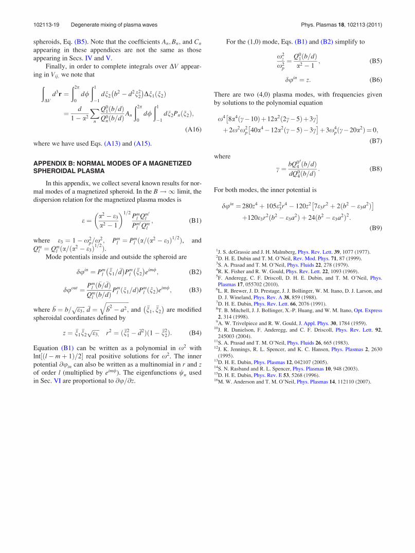
spheroids, Eq. (B5). Note that the coefficients An;Bn; and Cn

appearing in these appendices are not the same as those

appearing in Secs. IV and V.

Finally, in order to complete integrals over DV appear-

ing in Vij; we note thatðDV

d3r ¼ð2p

0

d/ð1

�1

dn2 b2 � d2n22

�Dn1 n2ð Þ

¼ d

1� a2

Xn

Q01ðb=dÞ

Q0nðb=dÞAn

ð2p

0

d/ð1

�1

dn2Pnðn2Þ;

(A16)

where we have used Eqs. (A13) and (A15).

APPENDIX B: NORMAL MODES OF A MAGNETIZEDSPHEROIDAL PLASMA

In this appendix, we collect several known results for nor-

mal modes of a magnetized spheroid. In the B!1 limit, the

dispersion relation for the magnetized plasma modes is

e ¼ a2 � e3

a2 � 1

� 1=2Pm

l Qm0l

Pm0l Qm

l

; (B1)

where e3 ¼ 1� x2p=x

2; Pml ¼ Pm

l ða=ða2 � e3Þ1=2Þ, and

Qml ¼ Qm

l ða=ða2 � e3Þ1=2Þ.Mode potentials inside and outside the spheroid are

duin ¼ Pml

�n1=�d �

Pml

�n2

�eim/; (B2)

duout ¼ Pml

�b=�dð ÞQm

l b=dð ÞPml n1=dð ÞPm

l n2ð Þeim/; (B3)

where �b ¼ b=ffiffiffiffiffiffie3;p �d ¼

ffiffiffiffiffiffiffiffiffiffiffiffiffiffiffiffi�b

2 � a2;

qand �n1; �n2

�are modified

spheroidal coordinates defined by

z ¼ �n1�n2

ffiffiffiffiffie3;p

r2 ¼ ð�n21 � �d2Þð1� �n2

2Þ: (B4)

Equation (B1) can be written as a polynomial in x2 with

lnt ðl� mþ 1Þ=2½ � real positive solutions for x2. The inner

potential @uin can also be written as a multinomial in r and zof order l (multiplied by eim/). The eigenfunctions wn used

in Sec. VI are proportional to @u=@z.

For the (1,0) mode, Eqs. (B1) and (B2) simplify to

x2z

x2p

¼ Q01ðb=dÞa2 � 1

; (B5)

duin ¼ z: (B6)

There are two (4,0) plasma modes, with frequencies given

by solutions to the polynomial equation

x4 8a4ðc�10Þþ12a2ð2c�5Þþ3c� þ2x2x2

p 40a4�12a2ðc�5Þ�3c�

þ3x4pðc�20a2Þ¼ 0;

(B7)

where

c ¼ bQ04

0ðb=dÞdQ0

4ðb=dÞ : (B8)

For both modes, the inner potential is

duin ¼ 280z4 þ 105e23r4 � 120z2 7e3r2 þ 2ðb2 � e3a2Þ

� þ120e3r2ðb2 � e3a2Þ þ 24ðb2 � e3a2Þ2:

(B9)

1J. S. deGrassie and J. H. Malmberg, Phys. Rev. Lett. 39, 1077 (1977).2D. H. E. Dubin and T. M. O’Neil, Rev. Mod. Phys. 71, 87 (1999).3S. A. Prasad and T. M. O’Neil, Phys. Fluids 22, 278 (1979).4R. K. Fisher and R. W. Gould, Phys. Rev. Lett. 22, 1093 (1969).5F. Anderegg, C. F. Driscoll, D. H. E. Dubin, and T. M. O’Neil, Phys.

Plasmas 17, 055702 (2010).6L. R. Brewer, J. D. Prestage, J. J. Bollinger, W. M. Itano, D. J. Larson, and

D. J. Wineland, Phys. Rev. A 38, 859 (1988).7D. H. E. Dubin, Phys. Rev. Lett. 66, 2076 (1991).8T. B. Mitchell, J. J. Bollinger, X.-P. Huang, and W. M. Itano, Opt. Express

2, 314 (1998).9A. W. Trivelpiece and R. W. Gould, J. Appl. Phys. 30, 1784 (1959).

10J. R. Danielson, F. Anderegg, and C. F. Driscoll, Phys. Rev. Lett. 92,

245003 (2004).11S. A. Prasad and T. M. O’Neil, Phys. Fluids 26, 665 (1983).12J. K. Jennings, R. L. Spencer, and K. C. Hansen, Phys. Plasmas 2, 2630

(1995).13D. H. E. Dubin, Phys. Plasmas 12, 042107 (2005).14S. N. Rasband and R. L. Spencer, Phys. Plasmas 10, 948 (2003).15D. H. E. Dubin, Phys. Rev. E 53, 5268 (1996).16M. W. Anderson and T. M. O’Neil, Phys. Plasmas 14, 112110 (2007).

102113-19 Degenerate mixing of plasma waves Phys. Plasmas 18, 102113 (2011)