Deformation Quantization and Cohomologies of Poisson, Graded, …€¦ · Deformation Quantization...
186
Deformation Quantization and Cohomologies of Poisson, Graded, and Homotopy algebras THESIS Presented on 12 November 2008 in Luxembourg by Mourad Ammar Born on 19 January 1980 in Sfax (Tunisia) In order to receive the academic degree of DOCTOR IN MATHEMATICS OF THE UNIVERSITY OF LUXEMBOURG and OF THE PAUL-VERLAINE UNIVERSITY IN METZ Doctoral committee Prof. Dr Didier ARNAL, Referee University of Bourgogne, France Prof. Dr Martin BORDEMANN, Referee University of Haute-Alsace Mulhouse, France Prof. Dr Simone GUTT, Advisor The Paul-Verlaine University in Metz, France Prof. Dr Yvette KOSMANN-SCHWARZBACH, President École Polytechnique, Paris, France Prof. Dr Pierre LECOMTE, Referee University of Liège, Belgium Prof. Dr Norbert PONCIN, Advisor University of Luxembourg, Luxembourg
Transcript of Deformation Quantization and Cohomologies of Poisson, Graded, …€¦ · Deformation Quantization...

Deformation Quantizationand
Cohomologies ofPoisson, Graded, and Homotopy
algebras
THESISPresented on 12 November 2008 in Luxembourg
by
Mourad AmmarBorn on 19 January 1980 in Sfax (Tunisia)
In order to receive the academic degree of
DOCTOR IN MATHEMATICSOF THE UNIVERSITY OF LUXEMBOURG
and
OF THE PAUL-VERLAINE UNIVERSITY IN METZ
Doctoral committee
Prof. Dr Didier ARNAL, RefereeUniversity of Bourgogne, France
Prof. Dr Martin BORDEMANN, RefereeUniversity of Haute-Alsace Mulhouse, France
Prof. Dr Simone GUTT, AdvisorThe Paul-Verlaine University in Metz, France
Prof. Dr Yvette KOSMANN-SCHWARZBACH, PresidentÉcole Polytechnique, Paris, France
Prof. Dr Pierre LECOMTE, RefereeUniversity of Liège, Belgium
Prof. Dr Norbert PONCIN, AdvisorUniversity of Luxembourg, Luxembourg


Acknowledgements
This work benefited from the encouragement of many. So let me acknowledge mygratitude to those who inspired and who supported me throughout these 4 years, tothose who pushed me to think harder and go further, and to all those who just werethere when I needed them to be there.
My first thoughts therefore go out to Professor Simone Gutt. Thanks to yourgreat support and all your encouragement, this work has had all the success I couldhave hoped and wished for. Thank you, Simone, for having enthused me to takethe road I travel by and for making this the difference.
My second special thank you is dedicated to Professor Norbert Poncin. Thankyou, Norbert, for this good training, your advice, your stimulation and understand-ing. What can I say when words are not enough to express all the gratitude I oweyou. We both know that this work is what it is thanks to you. And for this I oweyou my deepest respect and humblest THANK YOU.
Thirdly, I wish to thank those who supported my work over the years andwho, through their intellectual contribution, pushed me to think further: Profes-sors Véronique Chloup and Mohsen Mahsmoudi, as well as the belated ProfessorGuy Kass whom we all miss dearly.
A warm and hearty thank you to the referees and the members of the jury: Pro-fessors Didier Arnal, Martin Bordemann, Pierre Lecomte and Martin Schlichen-maier, as well as to Professor Yvette Kosmann-Schwarzbach who accepted to chairthe doctoral committee. Thank you for all the time you invested in me, for the faithyou gave to my work and to my abilities.
Lastly, on a more personal note, to my parents and brothers, whom I love, thankyou for your enduring support and unconditional love.
To all my friends and colleagues in Luxembourg and Metz, for your friendship,all the discussions and the assistance, I owe you my gratitude.
Thank you to the Universities of Luxembourg and Metz for welcoming me inyour warmest way. A special thank you to the Luxembourg mathematics researchunit for having supported me financially and, thus giving me the opportunity towork in a such wonderful team.
And, finally, for her love and support, for the inspiration and the improvements,thank you, Melanie, for being as wonderful as you are.

2

Contents
1 Introduction 71.1 General framework . . . . . . . . . . . . . . . . . . . . . . . . . 7
1.1.1 Deformation Quantization . . . . . . . . . . . . . . . . . 71.1.2 Poisson Geometry . . . . . . . . . . . . . . . . . . . . . 81.1.3 Investigated topics . . . . . . . . . . . . . . . . . . . . . 9
1.2 Developments, questions, results . . . . . . . . . . . . . . . . . . 91.2.1 Graded and strongly homotopy algebraic structures . . . . 91.2.2 Universal star product . . . . . . . . . . . . . . . . . . . 101.2.3 Poisson and Koszul cohomologies . . . . . . . . . . . . . 12
2 Loday Infinity Category 152.1 Introduction . . . . . . . . . . . . . . . . . . . . . . . . . . . . . 152.2 Canonical elements of graded Lie algebras . . . . . . . . . . . . . 18
2.2.1 Definitions, cohomology and formal deformations . . . . 182.2.2 Examples . . . . . . . . . . . . . . . . . . . . . . . . . . 23
2.3 Noncoassociative Tensor coalgebra . . . . . . . . . . . . . . . . . 262.4 Stem bracket . . . . . . . . . . . . . . . . . . . . . . . . . . . . 352.5 Graded and strongly homotopy Loday structures . . . . . . . . . . 382.6 Minimal model theorem for Loday infinity algebras . . . . . . . . 432.7 Graded and homotopy algebra cohomologies . . . . . . . . . . . 47
2.7.1 Graded Loday and Chevalley-Eilenberg cohomologies . . 472.7.2 Graded Poisson and Jacobi cohomologies . . . . . . . . . 482.7.3 Strongly homotopy and graded p-ary Loday cohomologies 58
3 L∞ algebras and deformation Quantization 613.1 Lie infinity algebras and their morphisms . . . . . . . . . . . . . 613.2 Generalized Maurer Cartan Equation . . . . . . . . . . . . . . . . 653.3 Twisted L∞ quasi-isomorphisms . . . . . . . . . . . . . . . . . . 68
3

4 CONTENTS
3.4 Moduli space of L∞ algebras . . . . . . . . . . . . . . . . . . . . 703.4.1 Application: Moduli space of a canonical element . . . . 75
3.5 Deformation quantization of Poisson manifolds . . . . . . . . . . 763.5.1 Formal Poisson structure . . . . . . . . . . . . . . . . . . 773.5.2 Star products on Poisson manifold . . . . . . . . . . . . . 783.5.3 On the formality Theorem on Rd . . . . . . . . . . . . . . 81
4 Universal Star Products 894.1 Introduction . . . . . . . . . . . . . . . . . . . . . . . . . . . . . 894.2 An example at order 3 . . . . . . . . . . . . . . . . . . . . . . . . 914.3 Universal Poisson cohomology . . . . . . . . . . . . . . . . . . . 934.4 Grothendieck- and Dolgushev-resolution . . . . . . . . . . . . . . 974.5 Construction of a universal star product . . . . . . . . . . . . . . 1054.6 A universal formality L∞ quasi-isomorphism . . . . . . . . . . . . 106
5 Poisson Cohomology of Twisted Structures 1135.1 Introduction . . . . . . . . . . . . . . . . . . . . . . . . . . . . . 1135.2 Vertically positive double complex . . . . . . . . . . . . . . . . . 115
5.2.1 Definition . . . . . . . . . . . . . . . . . . . . . . . . . . 1155.2.2 Application to twisted r-matrix induced Poisson structures 116
5.3 Model of spectral sequences . . . . . . . . . . . . . . . . . . . . 1205.4 Formal cohomology of Poisson tensor Λ4 . . . . . . . . . . . . . 125
5.4.1 Computation of the second term of the SpecSeq . . . . . . 1265.4.2 Prolongable systems S(zqp;r) . . . . . . . . . . . . . . . 1275.4.3 Forecast . . . . . . . . . . . . . . . . . . . . . . . . . . . 1285.4.4 Computation through the SpecSeq . . . . . . . . . . . . . 1295.4.5 Limit of the SpecSeq and reconstruction of the cohomology 135
5.5 Formal cohomology of Poisson tensor Λ8 . . . . . . . . . . . . . 139
6 Koszul and Poisson cohomology 1436.1 Introduction . . . . . . . . . . . . . . . . . . . . . . . . . . . . . 1436.2 strongly r-matrix induced structures . . . . . . . . . . . . . . . . 145
6.2.1 Stabilizer dimension and r-matrix generation . . . . . . . 1456.2.2 Classification theorem in Euclidean Three-Space . . . . . 147
6.3 Poisson cohomology in finite-dimensional . . . . . . . . . . . . . 1526.3.1 Koszul homology and cohomology . . . . . . . . . . . . 1526.3.2 Poisson cohomology in dimension 3 . . . . . . . . . . . . 1536.3.3 Poisson cohomology in dimension n . . . . . . . . . . . . 154
6.4 Koszul cohomology . . . . . . . . . . . . . . . . . . . . . . . . . 162

CONTENTS 5
6.5 Koszul and Poisson cohomology . . . . . . . . . . . . . . . . . . 1686.6 Cohomology spaces of structures Λ3 and Λ9 . . . . . . . . . . . . 1746.7 Cohomological phenomena . . . . . . . . . . . . . . . . . . . . . 175
Bibliography. 179

6 CONTENTS

Chapter 1
Introduction
1.1 General framework
This thesis “Deformation Quantization and Cohomologies of Poisson, Graded, andHomotopy algebras” is located at the interface of Deformation Quantization andPoisson Geometry.
1.1.1 Deformation Quantization
When switching from the Hamiltonian model of Classical Mechanics to the usualmodel of Quantum Mechanics, we completely change the nature of the observ-ables. From functions on the phase space, we pass to operators on some Hilbertspace. The commutator bracket [−,−] of these operators substitutes for the classi-cal Poisson bracket −,− of functions.
The transition from Classical Mechanics to Quantum Mechanics is providedby Heisenberg’s rules. These rules entail the uncertainty principle and Dirac’sequation [ f , g] = ih f ,g, where f ,g are functions of the phase space,ˆdenotes thequantization map, and h is Planck’s constant. However, Van Hove’s theorem (1952)states that this quantization cannot be extended to all phase space functions—andeven not to all polynomials—, in such a way that Heisenberg’s rules and Dirac’sequation be still valid. The way out is to look for a quantization that verifies theweakened Dirac equation
[ f , g] = ih f ,g+hε(h), (1.1)
where ε(h) tends to 0 with h. Weyl’s quantization W meets both requirements,Heisenberg’s rules and Dirac’s weak equation. Indeed, it quantizes any monomial
7

8 CHAPTER 1. INTRODUCTION
in positions qα and momenta pα by the symmetrized product of the correspondingoperators qα and pα , which are of course given by Heisenberg’s rules. The mapW is not a homomorphism from classical to quantum observables, i.e. in generalW ( f .g) 6=W ( f )W (g), where . is the pointwise product. One observes that W ( f )W (g) = W ( f ?g). Here f ?g denotes the Moyal-Vey product
f ?g = f .g+ν f ,g+ ∑k≥2
νkck( f ,g), (1.2)
where ν = ih/2 and where the ck are bidifferential operators on the function space,say N, which vanish on constants and verify ck( f ,g) = (−1)kck(g, f ). It is noweasily seen that
[W ( f ),W (g)] = W ( f ?g−g? f ) = ihW ( f ,g)− ih3
4W (c3( f ,g))+ . . . , (1.3)
so that condition (1.1) is actually satisfied. Moreover, the Moyal ? product is a for-mal deformation of the associative algebra (N, .) and leads via antisymmetrizationto a formal deformation of the Poisson algebra (N,−,−).
A seminal idea of Flato is that our description of Physics, should evolve, whenfacing a paradox, to a higher level by means of an appropriate deformation. Inthis perspective, Bayen, Flato, Fronsdal, Lichnerowicz, and Sternheimer suggestaround 1975, in a founding article that appeared in “Annals of Physics”, to abandonthe representation of classical observables by linear operators, and to construct amodel of Quantum Mechanics via deformation of the algebraic structure of the ob-servable space N. Roughly speaking, the task is the construction, on any symplec-tic or Poisson manifold, of a ?-product similar to Moyal’s product. This ?-productthen allows endowing the space N[[ν ]] of all formal series in ν with coefficientsin N, with an associative noncommutative algebra structure, as well as with a Liealgebra structure; these algebras are formal deformations of (N, .) and (N,−,−)respectively. Hence, in Deformation Quantization, Quantum Mechanics appearsas a deformation of Classical Mechanics, as a deformation from commutativity tononcommutativity, such that the trace of noncommutativity on the classical level isthe Poisson bracket.
1.1.2 Poisson Geometry
Poisson Geometry is the geometry of Poisson manifolds, i.e. smooth manifoldsendowed with a bivector field that squares to zero under the Schouten-Nijenhuisbracket. This field allows defining Hamiltonian vector fields and thus leads to a

1.2. DEVELOPMENTS, QUESTIONS, RESULTS 9
general distribution, which turns out to be completely integrable. The Poissonstructure induces on each maximal integral submanifold a symplectic structure, sothat a Poisson manifold can be viewed as a smooth concatenation of symplecticmanifolds. Of course, a Poisson manifold can also be thought of as a smoothmanifold whose function space carries a Poisson bracket. Poisson structures werestudied by Poisson, Jacobi and Lie, then by Kirillov and Lichnerowicz.
As from the 1970’s, Poisson Geometry developed rapidly with connectionswith many fields of Mathematics and Theoretical Physics, such as variational cal-culus, geometric mechanics, noncommutative algebra, representation theory.
1.1.3 Investigated topics
There exist tight connections between Poisson Geometry and Deformation Quan-tization. First, Poisson Geometry is inter alia the natural frame of DeformationQuantization. Moreover, investigations on existence and uniqueness of starproducts on symplectic or Poisson manifolds are related with associative, Lie,Poisson, and strongly homotopy algebras, as well as with the correspondingHochschild, Chevalley-Eilenberg, and Poisson-Lichnerowicz cohomologies.
This thesis is motivated by those connections. We study:-graded and strongly homotopy algebraic structures (defining a Tensor Coal-
gebra for Graded Loday and Lod∞ Structures which gives a unification for Gradedand Infinity Cohomologies),
-Poisson and Koszul cohomologies (Formal Poisson cohomology of twisted r-matrix induced structures; Strongly r-matrix induced tensors, Koszul cohomology,and arbitrary-dimensional quadratic Poisson cohomology),
- universal star products on Poisson manifolds.
1.2 Developments, questions, results
1.2.1 Graded and strongly homotopy algebraic structures
In 1993, Stasheff, [Sta93], identified the Hochschild (resp. Chevalley-Eilenberg)cochain space with coderivations of the tensor (resp. symmetric tensor) coalge-bra of the shifted underlying vector space, and observed that the Gerstenhaber(resp. Nijenhuis-Richardson) graded Lie bracket can be built from the commutatorbracket of coderivations. Further, associative (resp. Lie) structures correspond toodd quadratic codifferentials. When replacing quadratic codifferentials with arbi-trary odd codifferentials, we recover the concept of strongly homotopy associative
10 CHAPTER 1. INTRODUCTION
or A∞ (resp. strongly homotopy Lie or L∞) algebra, see [Sta63] (resp. [SS85]).These algebras had originally been defined noncoalgebraically by means of a se-quence of multilinear (resp. skew-symmetric multilinear) maps, which satisfy asequence of relations that encode the fact that A∞ (resp. L∞) algebras are asso-ciative (resp. Lie) algebras up to homotopy. Kontsevich, [Kon03], described L∞algebras in terms of formal Q-manifolds, a view that allows proving proprieties ofL∞ algebras via geometric arguments.
The operadic theory, as developed in [MSS02], shows that the Stasheff’sapproach works on any quadratic operad P . One associates a cofree (nilpotent)coalgebra over the dual operad whose quadratic codifferentials correspond tothe P−algebra structures on a graded vector space V . This result produces thehomology or cohomology theories of P−algebras on V and allows to definestrongly homotopy P−algebra structures on V as arbitrary codifferentials.
In this thesis we give an explicit coalgebraic approach to graded Loday andLoday infinity algebras, as well as to the corresponding cohomology theories.
Chapter 2 is devoted to these and related questions. We define a graded non-coassociative coproduct on the tensor space TW of any Zn–graded vector space W .If W is the desuspension space ↓ V of a graded vector space V , the coderivations(resp. codifferentials, quadratic codifferentials) of this coalgebra are 1-to-1 withsequences πs, s ≥ 1, of s-linear maps (resp. Loday infinity structures, Zn–gradedLoday structures) on V . We prove a minimal model theorem for Loday infinity al-gebras, investigate Loday infinity morphisms, and observe that the Lod∞ categorycontains the L∞ category as a subcategory. Moreover, the graded Lie bracket ofcoderivations gives rise to a graded Lie “stem” bracket on the cochain spaces ofgraded Loday and Loday infinity algebras. These algebraic structures have squarezero with respect to the stem bracket, so that we obtain natural cohomological the-ories that have good properties with respect to deformations. The stem bracketrestricts to the graded Nijenhuis-Richardson and Grabowski-Marmo brackets (thelast bracket extends the Schouten-Nijenhuis bracket to the space of graded firstorder differential operators), and it encodes the cohomologies of graded Loday,graded Lie, graded Poisson, graded Jacobi, Loday infinity, Lie infinity, as well asthat of p-ary graded Lie algebras in the sense of Michor and Vinogradov.
1.2.2 Universal star product
In [Kon03], Kontsevich proved his formality theorem onRd by explicitly determin-ing an L∞ morphism from the differential graded Lie algebra (DGLA) Tpoly(Rd)

1.2. DEVELOPMENTS, QUESTIONS, RESULTS 11
of polyvector fields on Rd to the DGLA Dpoly(Rd) of polydifferential operatorson Rd . The corestriction maps of this morphism, which are multilinear gradedskew-symmetric maps from Tpoly(Rd) to Dpoly(Rd), associate to each collectionof polyvector (resp. bivector) fields, a sequence of polydifferential (resp. bidif-ferential) operators. If in this collection each bivector field coincides with a samePoisson bivector, the resulting bidifferential operators are the coefficients of a starproduct on Rd . Kontsevich then proved the existence of star products on a generalPoisson manifold M by abstract gluing arguments that originate from the Gelfand-Kazhdan [GK71] formal geometry.
In [CFT02], Cattaneo, Felder and Tomassini proposed another globalizationprocedure for M. They observed that the so-called Grothendieck connection DG
on the jet bundle E →M can be used to build, in a spirit similar to Fedosov’s con-struction, a flat connection D on E that allows transferring Kontsevich’s fiberwizequantization to the base M.
Later on, in [Dol05], Dolgushev globalizes Kontsevich’s L∞ morphism to anarbitrary smooth manifold M. He constructs “à la Fedosov" a flat connection DF
on the jet bundle E → M, which gives rise to a resolution of the function alge-bra C∞(M) by differential forms on M valued in the sections of E. This resolutioninduces a resolution of the space of polyvectors fields (resp. polydifferential opera-tors) on M by differential forms on M with values in the bundle of formal fiberwizepolyvector fields (resp. polydifferential operators). The fiberwize Kontsevich L∞morphism is then twisted and contracted to yield an L∞ morphism from Tpoly(M)to Dpoly(M).
In this thesis, we took an interest in the comparison of the star products imple-mented by the globalization procedures of [CFT02] and [Dol05], motivated by thequest of an intrinsic way to characterize and parameterize (at least in lower orders)some star products on a Poisson manifold.
Chapter 3 contains the needed preliminaries. We analyze the role of L∞ al-gebras in deformation theory and review Kontsevich’s formality theorem togetherwith his star product formula. Further, we detail some algebraic proofs concerningL∞ algebras that cannot easily be found in the literature.
In Chapter 4, we define the concept of universal formality L∞ morphism: Forany manifold M and any torsion-free linear connection on M, a universal formal-ity L∞ morphism is an L∞ morphism from the DGLA Tpoly(M) to the DGLADpoly(M), such that the corestriction maps associate to each collection of polyvec-tor fields a collection of polydifferential operators, whose coefficients are tensors

12 CHAPTER 1. INTRODUCTION
given by universal polynomial expressions in the considered fields, the curvaturetensor R and the covariant iterated derivatives. Existence of such a morphism isdeduced from Dolgushev’s formality globalization. It implies in particular theexistence of a universal deformation quantization. Similarly, we stress that theglobalization procedure of [CFT02] also induces a universal deformation quanti-zation. We compare these procedures and prove that the Grothendieck connectionDG and the Fedosov-Dolgushev connection DF , coincide. We show that universalquantizations essentially are unique up to order 3 in the deformation parameter, bycomputing the appropriate universal Poisson cohomology.
The results are published in [ACG08].
1.2.3 Poisson and Koszul cohomologies
Since Poisson cohomology computations are known to be quite difficult, many pa-pers study the Euclidean plane or specific cases. In [MP06], the authors provide ageneral approach to Poisson cohomology of a broad set of isomorphism classes ofthe Dufour-Haraki classification for quadratic Poisson tensors of Euclidean three-space, [DH91]. More precisely, this quite powerful cohomological technique ap-plies to all r-matrix induced Poisson tensors and allowed discovering main aspectsof the structure of Poisson cohomology.
Hence, the questions whether it might be possible to construct a cohomologi-cal modus operandi for the more demanding remaining isomorphism classes andto understand the impact of the deviation from r-matrix implementation on thecohomological structure.
The answers to these questions are detailed in Chapter 5. More precisely,quadratic Poisson tensors of the Dufour-Haraki classification read as a sum of anr-matrix induced structure twisted by a (small) compatible exact quadratic tensor.This splitting is a remote variant of Liu and Xu’s decomposition theorem. Analgebraic bidegree of the space of formal Poisson cochains, that differs with thegeometric bigrading used by Vaisman in the regular case, then leads to a verti-cally positive double complex. The associated spectral sequence allows to com-pute the Poisson-Lichnerowicz cohomology of the considered tensors. We depictthis modus operandi, apply our technique to concrete examples of twisted Poissonstructures, and obtain a complete description of their cohomology. Since richnessof Poisson cohomology entails computation through the whole spectral sequence,we detail an entire model of this sequence. Finally, the chapter corroborates thatlargeness of Poisson cohomology can be viewed as a measure for deficiency of theconsidered Poisson tensor to be Koszul-exact.

1.2. DEVELOPMENTS, QUESTIONS, RESULTS 13
The results are published in [AP07].
The methods presented in [MP06] and [AP07] allow computing the cohomol-ogy of any three-dimensional quadratic Poisson tensor. Hence, it seems naturalto examine to which extent these techniques may be generalized to higher dimen-sional spaces.
In Chapter 6, we introduce the concept of strongly r-matrix induced (SRMI)Poisson structure, report on the relation of this property with the stabilizer dimen-sion of the considered quadratic Poisson tensor, and classify the Poisson structuresof the Dufour-Haraki classification (DHC) according to their membership of thefamily of SRMI tensors. One of the main results of this work is a generic co-homological procedure for SRMI Poisson structures in arbitrary dimension. Thisapproach allows decomposing Poisson cohomology into, basically, a Koszul co-homology and a relative cohomology. Moreover, we investigate this associatedKoszul cohomology, highlight its tight connections with Spectral Theory, and re-duce the computation of this main building block of Poisson cohomology to aproblem of linear algebra. We apply this to two structures of the DHC and pro-vide an exhaustive description of their cohomology. We thus complete the list ofdata obtained in previous works, see [MP06] and [AP07]. This deepens our insightinto the structure of Poisson cohomology, in particular as concerns Casimirs andthe cohomological impact of the singularities and the stabilizer of the consideredPoisson tensor.

14 CHAPTER 1. INTRODUCTION

Chapter 2
Coalgebraic Approach to theLoday Infinity Category,Stem Differential for 2p-aryGraded and Homotopy Algebras
2.1 Introduction
Our initial investigations on deformation quantization of Poisson manifolds in-spired us to explore two notions: the concept of strongly homotopy Lie algebrasor L∞ algebras, which plays a crucial role in Kontsevich’s work [Kon03] on theexistence of star products on a Poisson manifold and on the classification of theseproducts; the second notion is that of Poisson cohomology, which appears in theproblem of uniqueness of star products.
When realizing that an L∞ [SS85] structure is a codifferential of a certain coal-gebra, and that Poisson cohomology can be derived as a particular case of moregeneral cohomologies of algebras, we first concentrated on studying the conceptsof coalgebras and of cohomologies.
As our comprehension progressed, we understood that coalgebras provide aframework that allows constructing the appropriate cohomology theory of a givenalgebraic structure. To sum it up briefly, the technique consists in the identificationof the cochain space of the investigated algebra with certain coderivations, in sucha way that the algebraic structure can be identified to a homogenous odd quadraticcodifferential. These identifications enable constructing a graded Lie bracket on
15

16 CHAPTER 2. LODAY INFINITY CATEGORY
the space of cochains by transfer of the commutator bracket of coderivations.The considered algebraic structures are then canonical elements of the transferredbracket, i.e. they square to zero with respect to this bracket. This proprietyallows defining a natural cohomology operator for the algebraic structure, namelythe adjoint action of this structure with respect to the transferred graded Liebracket. These canonical coboundary operators have excellent properties as faras deformation theory is concerned. The procedure was first applied by Stasheff[Sta93] in the case of associative and Lie algebras.
In [MSS02], the authors generalize the Stasheff approach to any arbitraryquadratic operad P . The chain complex for the homology or cohomology ofP−algebras on a graded vector space V is defined by means of constructing of acofree (nilpotent) coalgebra over the dual operad, whereby quadratic codifferen-tials correspond to the P−algebra structures on V . This naturally leads to definestrongly homotopy P−algebra structures on V as arbitrary codifferentials.
In the present work we provide explicitly a tensor coalgebra that induces theproper concepts of Loday infinity algebras and morphisms, and use Stasheff’smodus operandi to define the cohomologies of Zn-graded Loday, Loday infinity,and 2p-ary graded Loday algebras. This leads to a graded Lie “stem” bracket, inwhich are encrypted, in addition to the preceding cohomologies, the coboundaryoperators of graded Lie, graded Poisson, graded Jacobi, Lie infinity, and 2p-arygraded Lie algebras [MV97].
This chapter is organized as follows.
In Section 2, we study the link between the cohomology induced by a canonicalelement in a graded Lie algebra with formal deformations of this element. Our in-vestigations extend similar properties for the adjoint Hochschild (resp. Chevalley-Eilenberg, Leibniz) cohomology and deformations of associative (resp. Lie, Lo-day) structures, which were proved in [Ger64] (resp. [NR67], [Bal96]), and recov-ered in [Bal97].
Section 3 contains the definition of a graded dual Leibniz coalgebra structure∆ on the tensor algebra T (W ) of a Zn-graded vector space W . We provide explicitformulæ for the reconstruction of coderivations and cohomomorphisms from theircorestriction maps.
In Section 4, we transfer the Zn-graded Lie bracket of coderivations of thementioned tensor coalgebra T (W ) of the desuspension space W :=↓ V of an un-derlying Zn-graded vector space V , and get a Zn+1-graded (resp. Zn-graded)

2.1. INTRODUCTION 17
Lie bracket on the Zn+1-graded vector space of weighted multilinear maps on V(resp. on the Zn-graded vector space of sequences of shifted weighted multilinearmaps on V ). We determine the explicit form of this pullback “stem” bracket andshow that its Zn+1-graded version coincides in the case of a nongraded underly-ing space V (resp. of graded skew-symmetric multilinear mappings on V ) withRotkiewicz’s bracket [Rot05] pertaining to left Loday structures [and correspondsto Balavoine’s bracket [Bal97] concerning right Loday structures] (resp. with thegraded Nijenhuis-Richardson bracket [LMS91]).
Codifferentials of our dual Leibniz coalgebra T (W ) are characterized in Sec-tion 5. We prove that Zn-graded Loday structures on V can be viewed as (resp. wedefine strongly homotopy Loday structures on V as) degree e1 := (1,0, . . . ,0) ∈Zn quadratic (resp. odd degree) codifferentials of (T (↓ V ),∆). Loday infinitystructures and Loday infinity morphisms are described in terms of sequences ofweighted multilinear maps that satisfy explicitly depicted sequences of constraints:our Lod∞ algebras are really differential graded Loday algebras up to homotopyand the Lod∞ category contains the L∞ category as a subcategory.
Loday infinity (quasi)-isomorphisms are investigated. In Section 6, we provea minimal model theorem for strongly homotopy Loday algebras, and deduce thatany Loday infinity quasi-isomorphism has a quasi-inverse – a theorem whose Lieinfinity counterpart plays a key-role in Deformation Quantization.
In Section 7 we deal with graded and strongly homotopy cohomologies. Zn-graded Loday [resp. strongly homotopy Loday] structures are canonical for theZn+1-graded [resp. Zn-graded] stem bracket, so that we obtain a natural coho-mology theory and an explicit coboundary operator. In the nongraded (resp. theantisymmetric) [resp. the Lie infinity] case, our Zn-graded Loday [resp. Lodayinfinity] cohomology operator coincides with the Loday (resp. graded Chevalley-Eilenberg) [resp. Lie infinity] differential given in [DT97] and [Bal97] (resp. in[LMS91]) [resp. in [Pen01] and [FP02]].
Further, graded Poisson and Jacobi cohomologies were defined purely alge-braically by Grabowski and Marmo in [GM03]. The authors prove existence anduniqueness of a Zn+1-graded Jacobi (resp. Poisson) bracket on the algebra of anti-symmetric graded first order polydifferential operators (resp. of graded polyderiva-tions). We compute this “Grabowski-Marmo” bracket explicitly and explain howthe corresponding cohomologies are induced by our stem bracket.
Finally, essentially two p-ary extensions of the Jacobi identity were investi-gated during the last decades. The first, see e.g. [Fil85], leads to the Nambu-Liestructure, see [Nam73], the second, see [MV97], [VV98], [VV01], will in this

18 CHAPTER 2. LODAY INFINITY CATEGORY
text be referred to as p-ary Lie structure. We define analogously p-ary (p even)Zn-graded Loday structures and their cohomology. These graded p-ary Loday al-gebras are special strongly homotopy Loday algebras, so that we have to prove thatthe two stem bracket induced cohomologies coincide.
2.2 Canonical elements of graded Lie algebras
2.2.1 Definitions, cohomology and formal deformations
At the beginning of this thesis, we briefly analyze the well-known fact that in agraded Lie algebra (GLA) (g,−,−), any element π ∈ g1, such that π,π = 0,generates a differential graded Lie algebra (DGLA) (g,−,−,∂π), ∂π = π,−,and a GLA in cohomology that allows controlling the formal deformations of π .
Unless otherwise stated, all vector spaces that we consider in this text arespaces over a fieldK of characteristic 0, and all graded vector spaces areZn-graded,n ∈ N∗. The Zn–degree deg(v) of a vector v or the Zn–weight deg( f ) of a gradedlinear map f are often denoted by the same symbol v or f . If v, f ∈Zn are two suchdegrees, we set 〈v, f 〉 = ∑i vi fi. A homogeneous vector or graded linear map w istermed odd, if 〈w,w〉 ∈ Z is an odd number.
Definition 1. A graded Lie algebra (g,−,−) (GLA) is a Zn−graded vectorspace g = ⊕α∈Zngα together with a bilinear bracket −,− : g× g −→ g thatsatisfies the following conditions:
1. −,− is compatible with the grading of g, i.e.
gα ,gβ ⊂ gα+β , ∀α,β ∈ Zn (2.1)
2. −,− is anticommutative, i.e.
a,b=−(−1)〈a,b〉b,a, (2.2)
for all homogeneous a,b ∈ g
3. Any homogeneous a,b,c ∈ g verify the Jacobi identity
a,b,c= a,b,c+(−1)〈a,b〉b,a,c (2.3)
Definition 2. We call canonical element of a graded Lie algebra (GLA)(V,−,−), any odd element π ∈V that verifies π,π= 0.

2.2. CANONICAL ELEMENTS OF GRADED LIE ALGEBRAS 19
Definition 3. A differential graded Lie algebra (g,d,−,−) (DGLA) is a GLAtogether with a graded linear map d : g−→ g that is a differential (i.e. d2 = 0) anda graded derivation of the graded Lie bracket,
da,b= da,b+(−1)〈deg(d),a〉a,d b. (2.4)
Proposition 1. Every GLA (g,−,−) equipped with a canonical element π is aDGLA (g,∂π ,−,−), where ∂π := π,−.
Proof. When applying the Jacobi identity (2.3) with a = b = π , we obtain2π,π,c = 0 and, as field K is of characteristic zero, π,π,c = 0, so that∂π is a differential. It is also a derivation of the Lie bracket:
∂πa,b = π,a,b= π,a,b+(−1)〈π,a〉a,π,b= ∂πa,b+(−1)〈π,a〉a,∂πb. (2.5)
Since coboundary operator ∂π has the form of a Hamiltonian vector field, wesometimes refer to it as a Hamiltonian differential.
Proposition 2. The cohomology space H(g,d,−,−) (or H(g) for short) ofany DGLA (g,d,−,−) is a GLA for the bracket that is canonically induced by−,−.
Proof. Obvious.
If the considered DGLA is implemented by a GLA (g,−,−) endowed witha canonical element π , we denote the corresponding cohomology GLA by Hπ(g).
Next, we investigate the links between deformations of a canonical element πof a GLA (g,−,−) and the cohomology algebra Hπ(g).
Definition 4. Let π be a canonical element of a GLA (g,−,−) and set
g[[ν ]] =⊕
α∈Zn
gα [[ν ]],
where gα [[ν]] is the space of formal power series in the formal parameter ν withcoefficients in gα . A formal power series
πν :=∞
∑i=0
ν iπi ∈ gdeg(π)[[ν ]] (2.6)

20 CHAPTER 2. LODAY INFINITY CATEGORY
with first term π0 = π is a formal deformation of the canonical element π , if itsquares to zero w.r.t. the natural extension of the bracket −,− to a bilinear mapof the space g[[ν ]], i.e. if
πν ,πν=∞
∑p=0
ν p ∑i+ j=p
πi,π j= 0. (2.7)
A formal deformation of order q of π is a formal series (2.6) that is truncated atorder q in ν and satisfies the condition
∑i+ j=p
πi,π j= 0, (2.8)
for each 1 ≤ p ≤ q. We refer to formal deformations of order 1 as infinitesimaldeformations.
Let us first focus on existence and construction of formal deformations.
Proposition 3. The degree 2deg(π) cohomology space H2deg(π)π (g) of the DGLA
implemented by a canonical element π of a GLA (g,−,−), contains the ob-structions to extension of formal deformations of order at least 1 to higher orderdeformations. In particular, if H2deg(π)
π (g) = 0, any formal deformation of orderq≥ 1 can be extended to a formal deformation of order q+1.
Proof. Assume that π admits a formal deformation πν of order q, q ≥ 1, andset
Ep := ∑i+ j=pi, j 6=0
πi,π j ∈ g2deg(π), 1≤ p≤ q+1. (2.9)
Note first that Condition (2.8) is equivalent to
Ep =−2∂π(πp), 1≤ p≤ q, (2.10)
since πp is of odd degree deg(πp) = deg(π).

2.2. CANONICAL ELEMENTS OF GRADED LIE ALGEBRAS 21
As for Eq+1, it is quite easy to see that it is a cocycle for ∂π . Indeed, we have
∂π(Eq+1) = ∑i+ j=q+1
i, j 6=0
∂π(πi,π j)
= ∑i+ j=q+1
i, j 6=0
∂ππi,π j+(−1)〈πi,π〉πi,∂ππ j
= 2 ∑i+ j=q+1
i, j 6=0
∂ππi,π j (∗)= − ∑
k+l+ j=q+1k,l, j 6=0
πk,πl,π j
=13 ∑
k+l+ j=q+1k,l, j 6=0
(−πk,πl,π j−πl,π j,πk−π j,πk,πl)
= 0,
where, at (∗), we used Equations (2.9) and (2.10).In order to extend deformation πν to order q + 1, we must find an element
πq+1 ∈ gdeg(π) that satisfies the condition Eq+1 = ∂π(−2πq+1), see Equation (2.10).Hence, cocycle Eq+1 has to be a coboundary. Consequently, the obstruction to theextension of the formal deformation πν of π to the order q+1 is a (nonvanishing)cohomology class Eq+1 in H2deg(π)
π (g).
In order to define the equivalence of two formal deformations of a same canon-ical element of a GLA, we need the following
Lemma 1. Let π be a canonical element of a GLA (g,−,−). Consider a formalseries
χν =∞
∑i=1
ν iχi (2.11)
with coefficients in g0. If πν is a formal deformation of π , then
exp(ad χν) πν
is a formal deformation of π as well.
Proof. Let us first remark that here exp denotes the exponential series and that
(ad χν)kπν = χνχν . . .χν ,πν . . .︸ ︷︷ ︸k
= ∑∞p=0 ν p ∑i1+...+ik+ j=pχi1χi2 . . .χik ,π j . . ..
(2.12)

22 CHAPTER 2. LODAY INFINITY CATEGORY
It follows that the coefficient of ν p in the exponential series over k is made up bya finite number of terms in gdeg(π); indeed, if k ≥ p + 1, at least one of the χi`vanishes. Moreover, the coefficient of ν0 contains only the term k = 0, and thus(exp(ad χν) πν)0 = π . Eventually, as ad χν is a derivation of the bracket −,−,we have
(ad χν)kπν ,πν= ∑r+s=kr,s≥0
Crk(ad χν)rπν ,(ad χν)sπν,
where Crk = k!
(k−r)!r! . Hence,
exp(ad χν)πν ,πν= exp(ad χν)πν , exp(ad χν)πν,
which completes the proof of the lemma.
Definition 5. Let π be a canonical element of a GLA (g,−,−). Two formaldeformations πν and π ′ν of π are said to be equivalent (resp. equivalent up to orderq, q≥ 1), if there is a formal series χν of type (2.11), such that
exp(ad χν) πν = π ′ν (resp. exp(ad χν) πν = π ′ν +O(νq+1)). (2.13)
A deformation πν of π is called trivial (resp. trivial up to order q, q ≥ 1), if πν isequivalent to π (resp. equivalent to π up to order q).
Proposition 4. Let π be a canonical element of a GLA (g,−,−). If the coho-mology space Hdeg(π)
π (g) vanishes, any formal deformation of π is trivial.
Proof. Let πν := π +∑∞i=1 ν iπi be a formal deformation of π . We first prove that
πν is trivial up to order 1, then we proceed by induction. Condition (2.8) impliesthat 2∂π(π1) = 0, i.e. that π1 is a cocycle; as Hdeg(π)
π (g) = 0, there exists a χ1 ∈ g0,such that π1 = ∂π(χ1). When setting χ(1)
ν = νχ1, we get
exp(ad χ(1)ν )πν = π +O(ν2).
Suppose now that πν is trivial up to order q (q≥ 1), or, equivalently, that thereexists a formal series
χ(q)ν =
∞
∑i=1
ν iχi
with coefficients in g0, such that
π ′ν := exp(ad χ(q)ν )πν = π +νq+1π ′q+1 +O(νq+2). (2.14)

2.2. CANONICAL ELEMENTS OF GRADED LIE ALGEBRAS 23
As above, since π ′ν is a deformation of π , 2∂π(π ′q+1) = 0, so that there is χ ′q+1 ∈ g0
that verifies π ′q+1 = ∂π(χ ′q+1). Set now
χ(q+1)ν := χ(q)
ν +νq+1χ ′q+1 and π ′′ν := exp(ad χ(q+1)ν )πν .
It follows from Equation (2.12) that
π ′′ν −π ′ν =−νq+1∂π(χ ′q+1)+O(νq+2).
Hence, π ′′ν = π +O(νq+2), which completes the proof.
Concerning infinitesimal deformations, i.e. first order formal deformations, itis easily seen from the above explanations that
Proposition 5. Infinitesimal deformations of a canonical element π of a GLA(g,−,−) are classified up to first order equivalence by H deg(π)
π (g).
2.2.2 Examples
Below, we give two basic examples of canonical elements of graded Lie algebras.
Associative graded algebras, graded Gerstenhaber algebra
Let us recall the
Definition 6. Let V = ⊕A∈ZnV A be a Zn-graded vector space. An associativegraded algebra structure on V is an associative bilinear map π : V ×V → V thatrespects the gradation, i.e. that verifies π(V A,V B)⊂V A+B.
We now define a Zn+1-graded Lie algebra, for which any associative gradedalgebra structure on the Zn-graded vector space V is a canonical element.
Set
M(V ) =⊕
(A,a)∈Zn×ZM(A,a)(V ),
where M(A,a)(V ) = 0 for all a≤−2, M(A,−1)(V ) = V A, and where for each a≥ 0,M(A,a)(V ) is the space of all (a + 1)-multilinear maps A : V×(a+1) → V that haveweight A. For notational ease multilinear maps and their weights are denoted, hereand below, by the same symbol.
It is known, see [LMS91], that the Zn+1-graded vector space M(V ) admits aZn+1-graded Lie algebra structure.

24 CHAPTER 2. LODAY INFINITY CATEGORY
Theorem 1. For any A ∈ M(A,a)(V ), B ∈ M(B,b)(V ), and vi ∈ V vi = M(vi,−1)(V ),i ∈ 1, . . . ,a+b+1, we set
jGB A(v1, . . . ,va+b+1) =
a+1
∑i=1
(−1)〈A,B〉+〈B,v1+...+vi−1〉+b(i−1) (2.15)
A(v1, . . . ,vi−1,B(vi, . . . ,vi+b),vi+b+1, . . . ,va+b+1).
Then,
1. The pair (M(V ), [−,−]G), where
[A,B]G = jGA B− (−1)〈(A,a),(B,b)〉 jG
B A,
is a Zn+1-graded Lie algebra.
2. A bilinear map π : V ×V → V of weight 0 ∈ Zn, i.e. a map π ∈ M(0,1)(V ),satisfies the condition [π,π]G = 0 if and only if π is an associative gradedalgebra structure on V .
Observe that for a non-graded vector space V , i.e. a vector space endowed withthe trivial gradation, the GLA (M(V ), [−,−]G) coincides with the Gerstenhaber(graded Lie) algebra of V . In the graded case, we refer to (M(V ), [−,−]G) as thegraded Gerstenhaber algebra of V .
Remark also that the associative graded algebra structures on V are exactlythe canonical elements of degree (0,1) of the graded Gerstenhaber algebra of V .If π is an associative graded multiplication on V , the cohomology Hπ(M(V )) ofthe DGLA induced by the canonical element π will be denoted in the sequel byH Ass
π (V ). In the non-graded case, it coincides with the adjoint Hochschild coho-mology of the associative algebra (V,π).
Graded Lie algebras, graded Nijenhuis-Richardson algebra
For any integer p ∈ N∗, let N(p) be the p–tuple (1, . . . , p). An unshuffleI = (i1, . . . , ik) (1 ≤ k ≤ p) is a naturally ordered subset of N(p), i.e. a subset,such that 1 ≤ i1 < .. . < ik ≤ p. The length of I will be denoted by |I|. If I and Jare two unshuffles, such that I ∩ J = /0, we set (I;J) = (i1, . . . , i|I|; j1, . . . , j|J|) andwe denote by I ∪ J the unique unshuffle that coincides with (I;J) as a set. Let(−1)(I;J) be the signature of the permutation (I;J) → I ∪ J. If V is a Zn-gradedvector space, we also set V(I;J) = (vi1 , . . . ,vi|I| ;v j1 , . . . ,v j|J|), v` ∈ V , and denote byεV (I;J) the Koszul sign (which is for any transposition V(`+1,`) →V(`,`+1) given by

2.2. CANONICAL ELEMENTS OF GRADED LIE ALGEBRAS 25
(−1)〈v`,v`+1〉) implemented by the permutation V(I;J) →VI∪J.
Consider now the Zn+1-graded vector subspace A(V ) of M(V ) made up by theZn-graded skew-symmetric multilinear maps
A(. . . ,vi,vi+1, . . .) =−(−1)〈vi,vi+1〉A(. . . ,vi+1,vi, . . .). (2.16)
As M(V ), theZn+1-graded vector space A(V ) admits aZn+1-graded Lie algebrastructure, see [LMS91].
Theorem 2. For any A ∈ A(A,a)(V ) and B ∈ A(B,b)(V ), we set
(iBA)(VN(a+b+1)) =
(−1)〈A,B〉 ∑I∪ J = N(a+b+1)
|I|= b+1, |J|= a
(−1)(I;J)εV (I;J)A(B(VI),VJ),
where notations such as VN(a+b+1) mean of course
VN(a+b+1) = (v1, . . . ,va+b+1), v` ∈V.
Then,
1. The pair (A(V ), [−,−]NR), where
[A,B]NR = iAB− (−1)〈(A,a),(B,b)〉iBA, (2.17)
is a Zn+1-graded Lie algebra.
2. A bilinear Zn-graded antisymmetric map π : V ×V → V of weight 0 ∈ Zn,i.e. π ∈ A(0,1)(V ), satisfies the condition [π,π]NR = 0 if and only if π definesa Zn-graded Lie bracket on V .
We refer to the Zn+1-graded Lie algebra (A(V ), [−,−]NR) as the gradedNijenhuis-Richardson algebra of V . The preceding theorem points out that theZn-graded Lie algebra structures on V are exactly the canonical elements of degree(0,1) of this graded Nijenhuis-Richardson algebra of V . If π is such a Zn-gradedLie structure on V , the cohomology Lie algebra Hπ(A(V )) of the DGLA inducedby the canonical element π will be denoted by H Lie
π (V ). In the non-graded case, itcoincides with the adjoint Chevalley-Eilenberg cohomology of (V,π).

26 CHAPTER 2. LODAY INFINITY CATEGORY
2.3 Noncoassociative Tensor coalgebra
Let us briefly recall some well-known facts. A graded coalgebra (C,∆) is agraded vector space C =
⊕α∈Zn Cα together with a coproduct ∆, i.e. a linear map
∆ : C →C⊗C that verifies ∆(Cα) ⊂⊕β+γ=α Cβ ⊗Cγ . A cohomomorphism from
(C,∆) to a graded coalgebra (C′,∆′) is a weight 0 linear map F : C → C′, suchthat ∆′F = (F ⊗F )∆. In this text, the tensor product of linear maps is definedby ( f ⊗g)(v1⊗ v2) = (−1)〈g,v1〉 f (v1)⊗g(v2), with self-explaining notations. Fur-ther, a homogeneous coderivation of (C,∆) is a linear map Q : C → C of weightdeg(Q) that satisfies the co-Leibniz identity ∆Q = (Q⊗ id+ id⊗Q)∆, where id isthe identity map of C. Weight α coderivations form a vector space CoDerα(C),and the space CoDer(C) =
⊕α∈Zn CoDerα(C) of all coderivations carries a natural
Zn-graded Lie algebra structure provided by the graded commutator bracket.
To any Zn-graded vector space V , we associate the (reduced) associativetensor algebra T (V ) =
⊕∞p=1V⊗p (the full tensor algebra includes the term
V⊗0 = K as well), which carries two natural gradings, the Z-gradation T (V ) =⊕∞p=1 T pV , T pV := V⊗p, and the Zn-gradation T (V ) =
⊕α∈Zn T (V )α , T (V )α :=⊕∞
p=1(TpV )α , (T pV )α =
⊕β1+...+βp=α V β1 ⊗ . . .⊗V βp . In the following, unless
differently stated, we view T (V ) as Zn-graded vector space.
Proposition 6. Let V be a Zn−graded vector space. The coproduct
∆ : T (V )−→ T (V )⊗
T (V ),
defined by
∆(v1⊗ . . .⊗ vp) = ∑I∪J=N(p−1)
I 6= /0
εV (I;J) VI⊗
VJ⊗ vp (v` ∈V, p≥ 1), (2.18)
provides a graded (noncoassociative) coalgebra structure on T (V ) and verifies
(id⊗
∆)∆ = (∆⊗
id)∆+(T⊗
id)(∆⊗
id)∆, (2.19)
where we used above-detailed notations and where T : T (V )⊗
T (V ) →T (V )
⊗T (V ) is the twisting map, which exchanges two elements of the Zn-graded
space T (V ) modulo the corresponding Koszul sign.

2.3. NONCOASSOCIATIVE TENSOR COALGEBRA 27
Proof. It suffices to develop the three terms of (2.19). The first one reads
(id⊗
∆)∆(v1⊗ . . .⊗ vp) = ∑I∪J=N(p−1)
I 6= /0
εV (I;J)VI⊗
∆(VJ⊗ vp)
= ∑I∪J=N(p−1)
I 6= /0
εV (I;J) ∑K∪L=J
K 6= /0
εV (K;L)VI⊗
VK⊗
VL⊗ vp
= ∑I∪K∪L=N(p−1)
I,K 6= /0
εV (I;K;L)VI⊗
VK⊗
VL⊗ vp ,
the second is equal to
(∆⊗
id)∆(v1⊗ . . .⊗ vp) = ∑J∪L=N(p−1)
J 6= /0
εV (J;L)∆(VJ)⊗
VL⊗ vp
= ∑J∪L=N(p−1)
J 6= /0
εV (J;L) ∑I∪K=J\ j|J|
I 6= /0
εV (I; K)VI⊗
VK ⊗ v j|J|
⊗VL⊗ vp
= ∑I∪K∪L=N(p−1)
i|I|<k|K|, I,K 6= /0
εV (I;K;L)VI⊗
VK⊗
VL⊗ vp
(J \ j|J| denotes J with j|J| omitted and K = (K, j|J|)), and for the third we get
(T⊗
id)(∆⊗
id)∆(v1⊗ . . .⊗ vp)
= ∑I∪K∪L=N(p−1)
i|I|<k|K|, I,K 6= /0
εV (I;K;L)(−1)〈VI ,VK〉VK⊗
VI⊗
VL⊗ vp
= ∑I∪K∪L=N(p−1)
k|K|<i|I|, I,K 6= /0
εV (K; I;L)(−1)〈VI ,VK〉VI⊗
VK⊗
VL⊗ vp
= ∑I∪K∪L=N(p−1)
k|K|<i|I|, I,K 6= /0
εV (I;K;L)VI⊗
VK⊗
VL⊗ vp .
Hence, the result.
The following theorem provides a characterization of the coderivations of thegraded coalgebra (T (V ),∆).

28 CHAPTER 2. LODAY INFINITY CATEGORY
Theorem 3. The mapping
ψVQ : CoDerQ(T (V )) 3 Q→ (Q1,Q2, . . .) =: ∑
pQp ∈ ∏
p≥1M(Q,p−1)(V ), (2.20)
which assigns to any (weight Q) coderivation Q its (weight Q) corestriction maps
Qp : T pV → T (V )Q−→ T (V )
pr−→ V, where pr denotes the canonical projection,is a vector space isomorphism, the inverse of which associates to any sequence(Q1,Q2, . . .) the coderivation Q that is defined by
Q(v1⊗ . . .⊗ vp) = (2.21)
∑I∪J∪K=N(p)
I,J<K
εV (I;J)(−1)〈Q,VI〉VI ⊗Q|J|+1(VJ⊗ vk1)⊗VK\k1 ,
where I < K means that i|I| < k1 and where v` ∈V v` .
Remark 1. The isomorphisms ψVQ , Q ∈ Zn, (for inverses, see Equation (2.21)),
induce an isomorphism ψV between CoDer(T (V )) and the corresponding directsum of direct products. Further, if we denote by CoDerQ
p (T (V )), Q ∈ Zn, p ∈ N∗,the image by (ψV
Q)−1 of M(Q,p−1)(V ), isomorphism ψVQ restricts to an isomorphism
ψV(Q,p) between these spaces. If no confusion arises, we write ψ instead of ψV , ψV
Q ,or ψV
(Q,p).
Proof. It suffices to show that Equation (2.21) defines a coderivation of degreeQ of the graded coalgebra (T (V ),∆), and that the thus defined map Ψ is the inverseof ψ , i.e. that its compositions with ψ coincide with the corresponding identitymaps.
Let us momentarily assume that Q verifies coderivation condition (2.3), so thatmap Ψ is actually valued in CoDerQ(T(V)). It is then easily seen that ψ Ψ = id.The second condition Ψ ψ = id then means that ψ is injective. So let us provethat if the corestriction maps of a coderivation Q vanish, then Q vanishes as well.
As ∆ vanishes if and only if its argument belongs to V , and as for any v ∈ V ,we have
∆Q(v) = (Q⊗
id)∆(v)+(id⊗
Q)∆(v) = 0,
it follows that Q(v) ∈ V . However, as Q1 = 0, we get Q(v) = 0, for any v ∈ V .Assume now that Q(v1⊗ . . .⊗ vk) = 0, v` ∈V , for any 1≤ k ≤ p−1 and proceedby induction. Since
∆(v1⊗ . . .⊗ vp) = ∑I∪J=N(p−1)
I 6= /0
εV (I;J) VI⊗
VJ⊗ vp,

2.3. NONCOASSOCIATIVE TENSOR COALGEBRA 29
we have
∆Q(v1⊗ . . .⊗ vp) = (Q⊗
id)∆(v1⊗ . . .⊗ vp)+(id⊗
Q)∆(v1⊗ . . .⊗ vp) = 0.
Consequently, Q(v1⊗ . . .⊗ vp) ∈ V and Q(v1⊗ . . .⊗ vp) = Qp(v1⊗ . . .⊗ vp) = 0.Eventually, Q actually vanishes, if its corestrictions vanish.
Let us now come to the core of the proof and show that the map Q defined byEquation (2.21) verifies the coderivation condition
∆Q(v1⊗ . . .⊗ vp) = (Q⊗
id+ id⊗
Q)∆(v1⊗ . . .⊗ vp), (2.22)
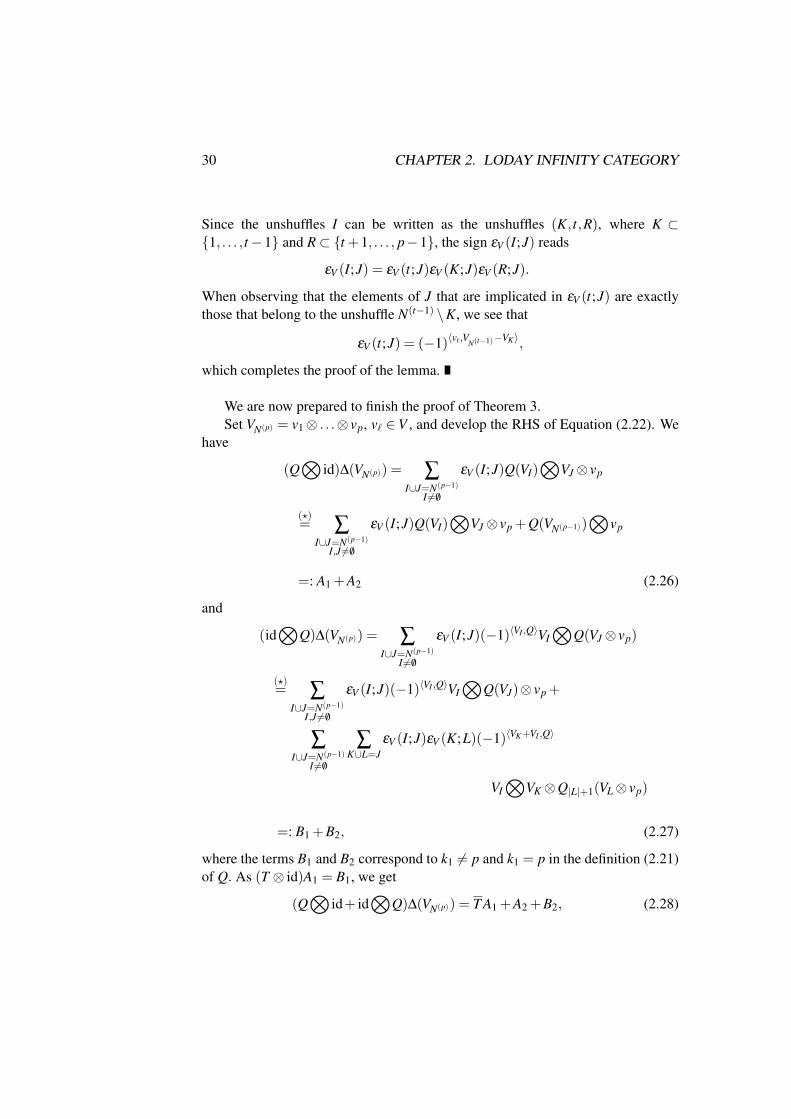
for any p≥ 1.Although this result is quite easily checked for p≤ 3, the general proof is rather
technical. It is better understood, if we are aware of the special role played by vp
in the definition of ∆. Thus, in the subsequent proof, we examine the terms of type
. . .Q(. . .⊗ vp) and . . .⊗
vp (2.23)
separately. Below, we refer to this idea as Remark (?).
The next lemma allows placing in the definition of ∆(v1⊗ . . .⊗ vt ⊗ . . .⊗ vp)any factor vt , t ∈ 1, . . . , p−1, on the left of
⊗and thus simplifies the comparison
the LHS and RHS of Equation (2.22).
Lemma 2. Set T = id+T ⊗ id, where T is the twisting map. For any fixed integert ∈ 1, . . . , p−1,
∆(v1⊗ . . .⊗ vt ⊗ . . .⊗ vp) = VN(p−1)
⊗vp + (2.24)
T ( ∑K∪R∪J=N(p−1)\t
K⊂1,...,t−1,R⊂t+1,...,p−1,J 6= /0
c VK ⊗ vt ⊗VR⊗
VJ⊗ vp),
with c = (−1)〈vt ,VN(t−1)−VK〉εV (K;J)εV (R;J).
Proof. We have
∆(v1⊗ . . .⊗ vt ⊗ . . .⊗ vp) = VN(p−1)
⊗vp +
∑I∪J=N(p−1)
t∈I, J 6= /0
εV (I;J)VI⊗
VJ⊗ vp + ∑I∪J=N(p−1)
t∈J, I 6= /0
εV (I;J)VI⊗
VJ⊗ vp
= VN(p−1)
⊗vp +T ( ∑
I∪J=N(p−1)
t∈I, J 6= /0
εV (I;J)VI⊗
VJ⊗ vp). (2.25)
30 CHAPTER 2. LODAY INFINITY CATEGORY
Since the unshuffles I can be written as the unshuffles (K, t,R), where K ⊂1, . . . , t−1 and R⊂ t +1, . . . , p−1, the sign εV (I;J) reads
εV (I;J) = εV (t;J)εV (K;J)εV (R;J).
When observing that the elements of J that are implicated in εV (t;J) are exactlythose that belong to the unshuffle N(t−1) \K, we see that
εV (t;J) = (−1)〈vt ,VN(t−1)−VK〉,
which completes the proof of the lemma.
We are now prepared to finish the proof of Theorem 3.Set VN(p) = v1⊗ . . .⊗ vp, v` ∈V , and develop the RHS of Equation (2.22). We
have
(Q⊗
id)∆(VN(p)) = ∑I∪J=N(p−1)
I 6= /0
εV (I;J)Q(VI)⊗
VJ⊗ vp
(?)= ∑
I∪J=N(p−1)
I,J 6= /0
εV (I;J)Q(VI)⊗
VJ⊗ vp +Q(VN(p−1))⊗
vp
=: A1 +A2 (2.26)
and
(id⊗
Q)∆(VN(p)) = ∑I∪J=N(p−1)
I 6= /0
εV (I;J)(−1)〈VI ,Q〉VI⊗
Q(VJ⊗ vp)
(?)= ∑
I∪J=N(p−1)
I,J 6= /0
εV (I;J)(−1)〈VI ,Q〉VI⊗
Q(VJ)⊗ vp +
∑I∪J=N(p−1)
I 6= /0
∑K∪L=J
εV (I;J)εV (K;L)(−1)〈VK+VI ,Q〉
VI⊗
VK ⊗Q|L|+1(VL⊗ vp)
=: B1 +B2, (2.27)
where the terms B1 and B2 correspond to k1 6= p and k1 = p in the definition (2.21)of Q. As (T ⊗ id)A1 = B1, we get
(Q⊗
id+ id⊗
Q)∆(VN(p)) = T A1 +A2 +B2, (2.28)

2.3. NONCOASSOCIATIVE TENSOR COALGEBRA 31
where
B2 = (2.29)
∑I∪K∪L=N(p−1)
I 6= /0
εV (I;K;L)(−1)〈VI+VK ,Q〉VI⊗
VK ⊗Q|L|+1(VL⊗ vp).
Let us now examine the LHS
∆Q(VN(p)) = (2.30)
∑M∪L∪S=N(p)
M,L<S
εV (M;L)(−1)〈VM ,Q〉∆(VM⊗Q|L|+1(VL⊗ vs1)⊗VS\s1)
of Equation (2.22).In this sum, the term C1 that corresponds to s1 = p, see Remark (?), reads
C1 = ∑M∪L=N(p−1)
M 6= /0
εV (M;L)(−1)〈VM ,Q〉∆(VM⊗Q|L|+1(VL⊗ vp)),
where unshuffle M is not empty, since term M = /0 vanishes, due to the fact that∆(v) = 0, for any v ∈V . The definition of ∆ yields
C1 =
∑M∪L=N(p−1)
M 6= /0εV (M;L)(−1)〈VM ,Q〉
∑I∪K=MI 6= /0
εV (I;K)VI⊗
VK ⊗Q|L|+1(VL⊗ vp) =
∑I∪K∪L=N(p−1)
I 6= /0εV (I;K;L)(−1)〈VI+VK ,Q〉VI
⊗VK ⊗Q|L|+1(VL⊗ vp),
which is exactly B2, see Equation (2.29).In view of Equation (2.28), it thus suffices to show that the remaining term C2
in Equation (2.30), which corresponds to s1 6= p, i.e.
C2 = ∑M∪L∪S=N(p−1)
M,L<S
εV (M;L)(−1)〈VM ,Q〉∆(VM⊗Q|L|+1(VL⊗ vs1)⊗VS\s1 ⊗ vp),
verifies
C2 = T A1 +A2. (2.31)

32 CHAPTER 2. LODAY INFINITY CATEGORY
When applying Lemma 2 with vt = Q|L|+1(VL⊗ vs1), we obtain
C2 =
∑M∪L∪S=N(p−1)
M,L<SεV (M;L)(−1)〈VM ,Q〉
VM⊗Q|L|+1(VL⊗ vs1)⊗VS\s1
⊗vp
+T (∑M∪L∪S=N(p−1)
M,L<S∑ K∪R∪J=M∪S\s1
K⊂M,R⊂S\s1, J 6= /0C VK ⊗Q|L|+1(VL⊗ vs1)⊗VR
⊗VJ⊗ vp),
where
C = (−1)〈VM ,Q〉(−1)〈VL+vs1+Q,VM−VK〉εV (M;L)εV (K;J)εV (R;J).
Equation (2.21) entails that the first term in C2 is nothing but A2. If D denotes thesecond term in C2, it suffices to prove that D = T A1.
Let us simplify D. The double sum in D is computed over unshufflesM,L,S,K,R,J, such that
(a)M∪L∪S = N(p−1), (b)K∪R∪ J = M∪S\s1,
(c)M < S, (d)L < S, (e)K ⊂M, ( f )R⊂ S\s1.
We now examine the impact of these conditions on C.
• Condition (b) implies that
εV (M;L) = εV (K;L)εV (R;L)εV (J;L)εV (S\s1;L).
• Conditions (d) and (f) imply that
εV (R;L)εV (S\s1;L) = (−1)〈VL,VS\s1+VR〉εV (L;R)εV (L;S\s1)
= (−1)〈VL,VS\s1−VR〉, (2.32)
since for any unshuffles I,J, where I < J, we have εV (I;J) = 1.
• Condition (f) implies that R = s1,R is an unshuffle. Then, in view of(2.32),
εV (M;L) = (−1)〈VL,VS\R〉εV (K;L)εV (J;L).

2.3. NONCOASSOCIATIVE TENSOR COALGEBRA 33
• Conditions (b), (e) and (f) imply that
J = (M\K)∪ (S\R) (2.33)
and so thatVJ = VM\K +VS\R.
Thus,εV (M;L) = (−1)〈VL,VJ−VM\K〉εV (K;L)εV (J;L).
When replacing in C, we get
C = (−1)〈VK ,Q〉(−1)〈vs1 ,VM\K〉(−1)〈VL,VJ〉εV (K;J;L)εV (R;J)= (−1)〈VK ,Q〉(−1)〈vs1 ,VM\K〉εV (K;L;J)εV (R;J).
Finally, when using (2.33) and (c), we obtain
εV (s1;J) = (−1)〈vs1 ,VM\K〉,
εV (R;J) = εV (s1;J)εV (R;J) = (−1)〈vs1 ,VM\K〉εV (R;J),
andC = (−1)〈VK ,Q〉εV (K;L;J)εV (R;J).
Hence,
D = T ( ∑K∪L∪R∪J=N(p−1)
K,L<R, J 6= /0
C VK ⊗Q|L|+1(VL⊗ vs1)⊗VR\s1
⊗VJ⊗ vp).
If we set now I = K∪L∪ R, we deduce that
C = (−1)〈VK ,Q〉εV (K;L)εV (I;J)
and, if we use again (2.21), we see that
D = T ( ∑I∪J=N(p−1)
I,J 6= /0
εV (I;J)Q(VI)⊗
VJ⊗ vp) = T A1.
Like coderivations, cohomomorphisms from (T (V ),∆) to (T (V ′),∆) are char-acterized by their corestriction maps.

34 CHAPTER 2. LODAY INFINITY CATEGORY
Theorem 4. Let V and V ′ be two Zn-graded vector spaces. A coalgebra coho-momorphism F : (T (V ),∆) −→ (T (V ′),∆) is uniquely defined by its (weight 0)corestriction maps Fp : T pV →V ′, p≥ 1, via the equation
F (v1⊗ . . .⊗ vp) =p
∑s=1
∑I1∪...∪Is=N(p)
I1,...,Is 6= /0i1|I1 |<...<is|Is|
εV (I1; . . . ; Is)F|I1|(VI1)⊗ . . .⊗F|Is|(VIs),
(2.34)where v` ∈V v` .
Proof. The proof of this theorem is similar to that of Theorem 3 and will notbe detailed here.
Set now e1 = (1,0, . . . ,0) ∈ Zn and consider the desuspension operator ↓ : V →↓V, where ↓V is the same space as V up to the shift (↓V )α = V α+e1 of gradation.The inverse map of ↓ is denoted by ↑. The mapping ↓⊗p:=↓ ⊗ . . .⊗ ↓, p factors,i.e. the mapping
↓⊗p: V⊗p 3 v1⊗ . . .⊗vp → (−1)∑ps=1〈(p−s)e1,vs〉 ↓ v1⊗ . . .⊗ ↓ vp ∈ (↓V )⊗p, (2.35)
is an isomorphism of weight −pe1, whose inverse is (−1)p(p−1)
2 ↑⊗p .
Remark 2. The isomorphisms
σ↓V(Q,p) : M(Q,p−1)(↓V ) 3 Qp → πp :=↑ Qp ↓⊗p∈M(Q+(1−p)e1,p−1)(V ), (2.36)
Q ∈ Zn, p ∈ N∗, (their inverses are defined by (−1)p(p−1)
2 ↓ πp ↑⊗p) generateisomorphisms σ↓V
Q and σ↓V between the corresponding direct products and directsums of direct products. If no confusion is possible, we omit super- and subscriptsand denote these isomorphisms simply by σ . Isomorphisms (2.36) extend of courseto multilinear maps on ↓V valued in ↓V ′.
Remark 3. Theorem 3-4 and Remarks1-2 show that weight Q coderivations Q :(T (↓V ),∆)→ (T (↓V ),∆) can be viewed as sequences π = (π1,π2, . . .) = ∑p πp ofweight Q+(1− p)e1 multilinear maps πp : V×p →V , and that cohomomorphismsF : (T (↓ V ),∆) → (T (↓ V ′),∆) (which by definition have weight 0) can be seenas sequences f = ( f1, f2, . . .) = ∑p fp of weight (1− p)e1 multilinear maps fp :V×p →V ′.

2.4. STEM BRACKET 35
2.4 Stem bracket
When combining the isomorphisms σ−1 and ψ−1, we get, for A ∈ Zn,a ∈ N, avector space isomorphism
φ(A,a) : M(A,a)(V ) 3 A→ QA = (0, . . . ,0,QAa+1,0, . . .) ∈ CoDerA+ae1
a+1 (T (↓V )),(2.37)
where QAa+1 = (−1)
a(a+1)2 ↓ A ↑⊗(a+1) and where QA is the coderivation that is
obtained from QAa+1 via extension equation (2.21).
Theorem 5. The Zn+1-graded vector space of multilinear maps Mr(V ) = M(V )ªV is a Zn+1-graded Lie algebra, when endowed with the bracket
[A,B]⊗ := (−1)1+〈ae1,be1+B〉φ−1(A+B,a+b)([φ(A,a)(A),φ(B,b)(B)]), (2.38)
A ∈M(A,a)(V ), B ∈M(B,b)(V ), where [−,−] denotes the Zn-graded Lie bracket ofthe space of coderivations of (T (↓V ),∆).
Proof. It follows from Equation (2.21) that the p-th corestrictionmap [φ(A,a)(A),φ(B,b)(B)]p vanishes if p 6= a + b + 1, so that the bracket
[φ(A,a)(A),φ(B,b)(B)] is really a coderivation in CoDerA+B+(a+b)e1a+b+1 (T (↓ V )). The
sign (−1)1+〈ae1,be1+B〉 ensures that the Zn-graded Lie bracket of coderivationsinduces a Zn+1-graded Lie bracket [−,−]⊗.
As the map φ = ψ−1 σ−1 is also a (weight 0) Zn-graded vector space isomor-phism
φ :C(V ) :=⊕
Q∈Zn∏p≥1
M(Q+(1−p)e1,p−1)(V )→CoDer(T (↓V ))=⊕
Q∈Zn
CoDerQ(T (↓V )),
(2.39)the next proposition is obvious.
Proposition 7. The Zn-graded vector space C(V ) of sequences of multilinear mapsis a Zn-graded Lie algebra for the bracket
[π,ρ]⊗ = φ−1[φπ,φρ ] = ∑q≥1
∑s+t=q+1
(−1)1+(s−1)〈e1,ρ〉[πs,ρt ]⊗, (2.40)
where π = ∑s πs ∈ Cπ(V ) and ρ = ∑t ρt ∈ Cρ(V ) are two homogeneous C(V )-elements of Zn-degree π and ρ respectively.
36 CHAPTER 2. LODAY INFINITY CATEGORY
Remark 4. In the following, we refer to [−,−]⊗ (resp. [−,−]⊗) as the Zn-graded(resp. Zn+1-graded) stem bracket.
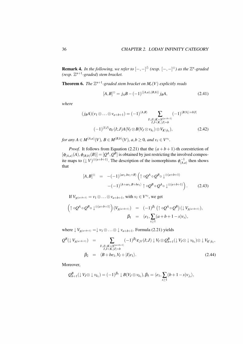
Theorem 6. The Zn+1-graded stem bracket on Mr(V ) explicitly reads
[A,B]⊗ = jAB− (−1)〈(A,a),(B,b)〉 jBA, (2.41)
where
( jBA)(v1⊗ . . .⊗ va+b+1) = (−1)〈A,B〉 ∑I∪J∪K=N(a+b+1)
I,J<K, |J|=b
(−1)〈B,VI〉+b|I|
(−1)(I;J)εV (I;J)A(VI ⊗B(VJ⊗ vk1)⊗VK\k1), (2.42)
for any A ∈M(A,a)(V ), B ∈M(B,b)(V ), a,b≥ 0, and v` ∈V v` .
Proof. It follows from Equation (2.21) that the (a + b + 1)-th corestriction of[φ(A,a)(A),φ(B,b)(B)] = [QA,QB] is obtained by just restricting the involved compos-ite maps to (↓ V )⊗(a+b+1). The description of the isomorphisms φ−1
(A,a) then showsthat
[A,B]⊗ = −(−1)〈ae1,be1+B〉(↑ QA QB ↓⊗(a+b+1)
−(−1)〈A+ae1,B+be1〉 ↑ QB QA ↓⊗(a+b+1))
. (2.43)
If VN(a+b+1) = v1⊗ . . .⊗ va+b+1, with v` ∈V v` , we get(↑ QA QB ↓⊗(a+b+1)
)(VN(a+b+1)) = (−1)β1
(↑ QA QB)(↓VN(a+b+1)),
β1 = 〈e1, ∑s≥1
(a+b+1− s)vs〉,
where ↓VN(a+b+1) =↓ v1⊗ . . .⊗ ↓ va+b+1. Formula (2.21) yields
QB(↓VN(a+b+1)) = ∑I∪J∪K=N(a+b+1)
I,J<K,|J|=b
(−1)β2ε↓V (I;J) ↓VI ⊗QBb+1(↓VJ⊗ ↓ vk1)⊗ ↓VK\k1 ,
β2 = 〈B+be1,VI + |I|e1〉. (2.44)
Moreover,
QBb+1(↓VJ⊗ ↓ vk1) = (−1)β3 ↓ B(VJ⊗ vk1),β3 = 〈e1, ∑
s≥1(b+1− s)v js〉,

2.4. STEM BRACKET 37
as the sign (−1)b(b+1)
2 inside QBb+1 and the sign due to the shift of the Zn-gradation
cancel each other out. When noticing that QA evaluated on an element of (↓V )⊗(a+1) is nothing but QA
a+1, we obtain
(↑ QA QB ↓⊗(a+b+1)
)(VN(a+b+1)) = (2.45)
∑I∪J∪K=N(a+b+1)
I,J<K, |J|=b
(−1)`ε↓V (I;J)A(VI ⊗B(VJ⊗ vk1)⊗VK\k1),
with ` = β1 +β2 +β3 +β4 +β5 +β6, where
β4 = 〈e1, ∑s≥1
(a+1−s)vis〉, β5 =(a−|I|)〈e1,B+VJ +vk1〉, and β6 = 〈e1, ∑s≥2
(a−|I|−s+1)vks〉
are generated by ↑⊗(a+1) and where, again, the sign inside QAa+1 and the sign due
to the shift neutralize.We will prove that
(−1)`ε↓V (I;J) = (−1)〈B,ae1〉+〈B,VI〉+b|I|(−1)(I;J)εV (I;J). (2.46)
Observe first that an appropriate regrouping of terms yields
` = `1 + `2 := (〈B,ae1〉+ 〈B,VI〉+b|I|)+
(〈e1,
a+b+1
∑s=1
(a+b+1− s)vs〉
+〈e1,|I|∑s=1
(a+b+1− s)vis〉+ 〈e1,|I|+|J|∑
s=|I|+1(a+b+1− s)v js−|I|〉
+〈e1,a+b+1
∑s=|I|+|J|+1
(a+b+1− s)vks−|I|−|J|〉)
,
where, since in view of the conditions I,J < K the concatenation (I;J) is a permu-tation of 1, . . . , |I|+ |J|, the term `2 reads (modulo even terms)
`2 = 〈e1,|I|∑s=1
(s+ is)vis〉+ 〈e1,|I|+|J|∑
s=|I|+1(s+ js−|I|)v js−|I|〉.
If permutation (I;J) is a transposition (I;J) = (1, . . . ,q−1,q+1,q,q+2, . . . , |I|+|J|), then `2 = 〈e1,vq + vq+1〉. It is now easily checked that for a transposition
(−1)`2ε↓V (I;J) = (−1)(I;J)εV (I;J) (2.47)

38 CHAPTER 2. LODAY INFINITY CATEGORY
and that for a composition of transpositions all the factors of this last equation arethe products of the corresponding factors induced by the involved transpositions.It follows that Equations (2.47) and (2.46) hold true for any permutation (I;J).
Eventually Equation (2.45) may be written(↑ QA QB ↓⊗(a+b+1)
)(VN(a+b+1)) =
∑I∪J∪K=N(a+b+1)
I,J<K, |J|=b
(−1)m(−1)(I;J)εV (I;J)A(VI ⊗B(VJ⊗ vk1)⊗VK\k1),
where m = 〈B,ae1〉+ 〈B,VI〉+b|I|.If we define the insertion operator
jBA = (−1)〈ae1+A,B〉 ↑ QA QB ↓⊗(a+b+1),
A ∈M(A,a)(V ), B ∈M(B,b)(V ), a,b≥ 0, we finally get the announced result.
Remark 5. It is easily checked that the restriction of the stem bracket [−,−]⊗
to the subspace Ar(V ) of Mr(V ), made up by graded skew-symmetric multilinearmaps on V , coincides with the graded Nijenhuis-Richardson bracket [−,−]NR.
2.5 Graded and strongly homotopy Loday structures
Let us recall that a codifferential of a coalgebra is a coderivation that squares to 0.
Proposition 8. A homogenous odd weight coderivation Q of the coalgebra(T (V ),∆) is a codifferential if and only if, for any p ≥ 1, the following equationholds identically:
∑I∪J∪K=N(p)
I,J<K
εV (I;J)(−1)〈Q,VI〉Q|I|+|K|(VI ⊗Q|J|+1(VJ⊗ vk1)⊗VK\k1) = 0. (2.48)
Proof. As Q is an odd weight coderivation, 2Q2 = [Q,Q] and so Q2 is also acoderivation. Thus, according to Theorem 3, the condition Q2 = 0 is satisfied ifand only if the corestriction maps Q2
p, p ≥ 1, of Q2 vanish. It is easily seen thatQ2
p(VN(p)) is exactly the LHS of (2.48).
Definition 7. A graded Loday algebra (g,−,−) (GLodA for short) is made upby a Zn-graded vector space g and a weight 0 bilinear bracket −,− that satisfiesthe graded Jacobi identity (2.3).
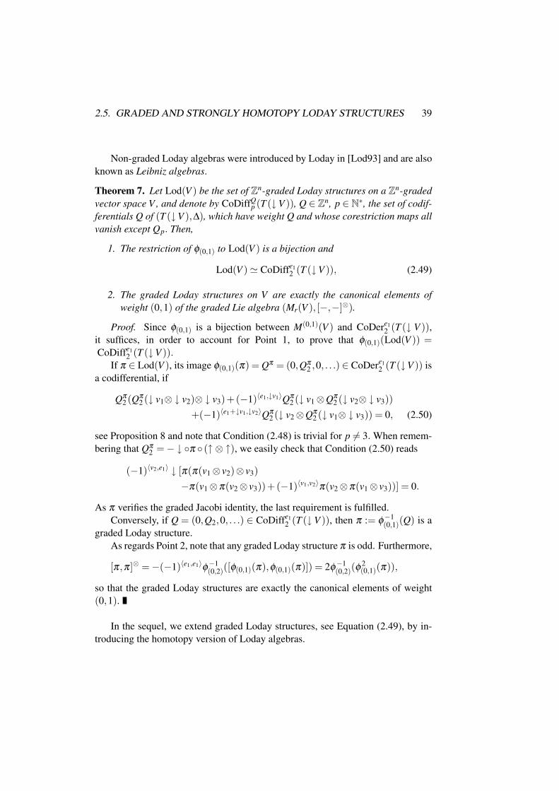
2.5. GRADED AND STRONGLY HOMOTOPY LODAY STRUCTURES 39
Non-graded Loday algebras were introduced by Loday in [Lod93] and are alsoknown as Leibniz algebras.
Theorem 7. Let Lod(V ) be the set of Zn-graded Loday structures on a Zn-gradedvector space V , and denote by CoDiffQ
p (T (↓V )), Q ∈ Zn, p ∈ N∗, the set of codif-ferentials Q of (T (↓V ),∆), which have weight Q and whose corestriction maps allvanish except Qp. Then,
1. The restriction of φ(0,1) to Lod(V ) is a bijection and
Lod(V )' CoDiffe12 (T (↓V )), (2.49)
2. The graded Loday structures on V are exactly the canonical elements ofweight (0,1) of the graded Lie algebra (Mr(V ), [−,−]⊗).
Proof. Since φ(0,1) is a bijection between M(0,1)(V ) and CoDere12 (T (↓ V )),
it suffices, in order to account for Point 1, to prove that φ(0,1)(Lod(V )) =CoDiffe1
2 (T (↓V )).If π ∈ Lod(V ), its image φ(0,1)(π) = Qπ = (0,Qπ
2 ,0, . . .) ∈ CoDere12 (T (↓V )) is
a codifferential, if
Qπ2 (Qπ
2 (↓ v1⊗ ↓ v2)⊗ ↓ v3)+(−1)〈e1,↓v1〉Qπ2 (↓ v1⊗Qπ
2 (↓ v2⊗ ↓ v3))+(−1)〈e1+↓v1,↓v2〉Qπ
2 (↓ v2⊗Qπ2 (↓ v1⊗ ↓ v3)) = 0, (2.50)
see Proposition 8 and note that Condition (2.48) is trivial for p 6= 3. When remem-bering that Qπ
2 =− ↓ π (↑ ⊗ ↑), we easily check that Condition (2.50) reads
(−1)〈v2,e1〉 ↓ [π(π(v1⊗ v2)⊗ v3)−π(v1⊗π(v2⊗ v3))+(−1)〈v1,v2〉π(v2⊗π(v1⊗ v3))] = 0.
As π verifies the graded Jacobi identity, the last requirement is fulfilled.Conversely, if Q = (0,Q2,0, . . .) ∈ CoDiffe1
2 (T (↓ V )), then π := φ−1(0,1)(Q) is a
graded Loday structure.As regards Point 2, note that any graded Loday structure π is odd. Furthermore,
[π,π]⊗ =−(−1)〈e1,e1〉φ−1(0,2)([φ(0,1)(π),φ(0,1)(π)]) = 2φ−1
(0,2)(φ2(0,1)(π)),
so that the graded Loday structures are exactly the canonical elements of weight(0,1).
In the sequel, we extend graded Loday structures, see Equation (2.49), by in-troducing the homotopy version of Loday algebras.

40 CHAPTER 2. LODAY INFINITY CATEGORY
Definition 8. A strongly homotopy Loday algebra or a Loday infinity algebra isa Zn-graded vector space V endowed with a codifferential of odd weight of thetensor coalgebra (T (↓V ),∆).
We denote by LodQ∞(V ), Q ∈ Zn, 〈Q,Q〉 odd, the set
LodQ∞(V )' CoDiffQ(T (↓V ))
of weight Q Loday infinity (LodQ∞ for short) structures on V , whereas Lod∞(V )
denotes the set Lode1∞ (V ) – as most infinity structures considered below have
weight e1. Since Q is odd, Q ∈ LodQ∞(V ) if and only if Q ∈ CoDerQ(T (↓ V )) and
[Q,Q] = 2Q2 = 0. Hence, in view of Remark 3 and Proposition 7, the sequencemaps “definition” of Loday infinity algebras:
Proposition 9. A Loday infinity algebra is a Zn-graded vector space V togetherwith a sequence of structure maps
π = (π1,π2, . . .) = ∑p
πp ∈CQ(V ) = ∏p≥1
M(Q+(1−p)e1,p−1)(V )
of odd degree Q, such that
∑s+t=p
(−1)1+(s−1)〈e1,Q〉[πs,πt ]⊗ = 0,∀p≥ 2. (2.51)
In the usual case of Lod∞ structures π on V , the first three conditions (2.51)mean that (V,π1) is a chain complex, that π1 is a Zn-graded derivation of the bilin-ear map π2, and that π2 is a Zn-graded Loday structure modulo homotopy π3.
Example 1. If the structure maps of a Lod∞ algebra (V,π) all vanish, except π1(resp. except π2, except π1 and π2), (V,π) is a chain complex (resp. a Zn-gradedLoday algebra (GLodA), a differential graded Loday algebra(DGLodA)).
Example 2. Let (V,π) and (V ′,π ′) be two Lod∞ algebras. Their direct sum (V ⊕V ′,π⊕π ′) is a Lod∞ algebra, where the structure maps are defined by
(π⊕π ′)p(v1 + v′1, . . . ,vp + v′p) := πp(v1, . . . ,vp)+π ′p(v′1, . . . ,v′p),
for any p≥ 1.
It is obvious from the structure of the explicit form of the stem bracket [−,−]⊗,see Theorem 6, that if π and π ′ verify the Lod∞ conditions (2.51) in V and V ′
respectively, then π⊕π ′ verifies the same conditions in V ⊕V ′.
As a Lod∞ structure on V is a weight e1 codifferential Q of the coalgebra (T (↓V ),∆), it is natural to give the following coalgebraic
2.5. GRADED AND STRONGLY HOMOTOPY LODAY STRUCTURES 41
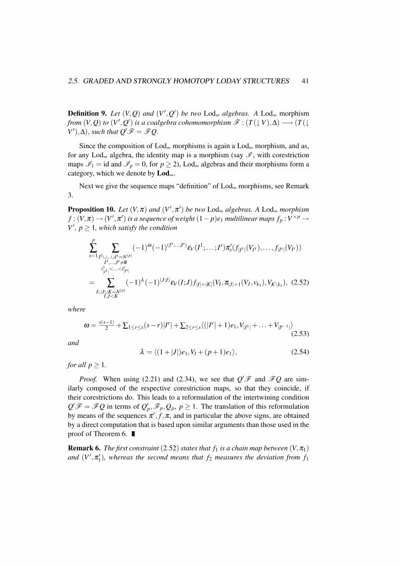
Definition 9. Let (V,Q) and (V ′,Q′) be two Lod∞ algebras. A Lod∞ morphismfrom (V,Q) to (V ′,Q′) is a coalgebra cohomomorphism F : (T (↓V ),∆)−→ (T (↓V ′),∆), such that Q′F = FQ.
Since the composition of Lod∞ morphisms is again a Lod∞ morphism, and as,for any Lod∞ algebra, the identity map is a morphism (say I , with corestrictionmaps I1 = id and Ip = 0, for p≥ 2), Lod∞ algebras and their morphisms form acategory, which we denote by Lod∞.
Next we give the sequence maps “definition” of Lod∞ morphisms, see Remark3.
Proposition 10. Let (V,π) and (V ′,π ′) be two Lod∞ algebras. A Lod∞ morphismf : (V,π)→ (V ′,π ′) is a sequence of weight (1− p)e1 multilinear maps fp : V×p →V ′, p≥ 1, which satisfy the condition
p
∑s=1
∑I1∪...∪Is=N(p)
I1,...,Is 6= /0i1|I1|<...<is|Is|
(−1)ω(−1)(I1;...;Is)εV (I1; . . . ; Is)π ′s( f|I1|(VI1), . . . , f|Is|(VIs))
= ∑I∪J∪K=N(p)
I,J<K
(−1)λ (−1)(J;I)εV (I;J) f|I|+|K|(VI,π|J|+1(VJ,vk1),VK\k1), (2.52)
where
ω = s(s−1)2 +∑1≤r≤s(s− r)|Ir|+∑2≤r≤s〈(|Ir|+1)e1,V|I1|+ . . .+V|Ir−1|〉
(2.53)and
λ = 〈(1+ |J|)e1,VI +(p+1)e1〉, (2.54)
for all p≥ 1.
Proof. When using (2.21) and (2.34), we see that Q′F and FQ are sim-ilarly composed of the respective corestriction maps, so that they coincide, iftheir corestrictions do. This leads to a reformulation of the intertwining conditionQ′F = FQ in terms of Q′
p,Fp,Qp, p ≥ 1. The translation of this reformulationby means of the sequences π ′, f ,π , and in particular the above signs, are obtainedby a direct computation that is based upon similar arguments than those used in theproof of Theorem 6.
Remark 6. The first constraint (2.52) states that f1 is a chain map between (V,π1)and (V ′,π ′1), whereas the second means that f2 measures the deviation from f1

42 CHAPTER 2. LODAY INFINITY CATEGORY
being a (V,π2)− (V ′,π ′2) homomorphism. If (V,π) and (V ′,π ′) are DGLodAs,map f1 is a DGLodA morphism. In Chapter 3, we shall recall the category L∞ ofL∞ algebras and morphisms and show that the category L∞ is a subcategory of
Lod∞.
Definition 10. A Lod∞ quasi-isomorphism from a Lod∞ algebra (V,π) to a Lod∞algebra (V ′,π ′) is a Lod∞ morphism f : (V,π) → (V ′,π ′), such that the chainmap f1 : (V,π1)→ (V ′,π ′1) induces an isomorphism f1 ] : H(V,π1)→ H(V ′,π ′1) incohomology. In particular, f is called a Lod∞ isomorphism, if f1 : V → V ′ is anisomorphism.
If F ' f and G ' g are two composable Lod∞ morphisms, we denote byg f the sequence of multilinear maps that corresponds to the Lod∞ morphismG F . Similarly, π ′ f and f π are the sequences that represent Q′F and FQ.The Lod∞ morphism condition (2.52) then reads π ′ f = f π. We use these andanalogous notations below.
The next proposition will be needed in the following.
Proposition 11. 1. Any coalgebra cohomomorphism f : (T (↓ V ),∆) → (T (↓V ′),∆), which corresponds to a sequence f = ( f1, f2, . . .), whose first elementf1 is bijective, is invertible, i.e. there is a coalgebra cohomomorphism f−1 :(T (↓V ′),∆)→ (T (↓V ),∆), such that f f−1 = Id and f−1 f = Id, whereId is the unit cohomomorphism Id = (id,0,0, . . .).
2. If (V,π) denotes a Lod∞ algebra, any sequence f = ( f1, f2, . . .) of weight(1− p)e1 multilinear maps fp : V×p →V , whose first element f1 is the iden-tity map of V , induces a new Lod∞ structure f π f−1 on V and f is a Lod∞isomorphism between (V,π) and (V, f π f−1).
3. Any Lod∞ isomorphism f : (V,π)→ (V ′,π ′) admits an inverse f−1 that is aLod∞ isomorphism as well.
Proof. 1. Let F : (T (↓ V ),∆) → (T (↓ V ′),∆) be a coalgebra cohomomor-phism, whose first corestriction F1 :↓ V →↓ V ′ is bijective. If there is an inversecohomomorphism G : (T (↓ V ′),∆) → (T (↓ V ),∆), it follows from the conditionFG = I and from Equation (2.34) that G1 = F−1
1 and that, for any p≥ 2,
Gp(↓ v′1, . . . ,↓ v′p)
=−p
∑s=2
∑I1∪...∪Is=N(p)
I1,...,Is 6= /0i1|I1 |<...<is|Is|
ε↓V ′(I1; . . . ; Is)F−11 Fs
(G|I1|(↓V ′
I1)⊗ . . .⊗G|Is|(↓V ′Is)
).

2.6. MINIMAL MODEL THEOREM FOR LODAY INFINITY ALGEBRAS 43
The last equation provides inductively the corestriction maps of a cohomomor-phism G . One can check that G not only verifies FG = I , but also G F = I .
2. Take a Lod∞ structure Q on V and a cohomomorphism F : (T (↓ V ),∆)→(T (↓V ),∆), such that F1 = id. Since ( f ⊗g) (h⊗k) = (−1)〈g,h〉( f h)⊗ (gk),with self-explaining notations, it is easily seen that FQF−1, where F−1 is theinverse cohomomorphism G given by Item 1, is a weight e1 codifferential of T (↓V ), i.e. a Lod∞ structure on V . Eventually, F is obviously a Lod∞ morphism, and,in view of the assumption F1 = id, even a Lod∞ isomorphism.
3. Consider two Lod∞ algebras (V,Q), (V ′,Q′) and a Lod∞ isomorphism F ,i.e. a cohomomorphism, such that F1 is bijective and Q′F = FQ (?). It thenfollows from Item 1 that there is an inverse cohomomorphism F−1, such that(F−1)1 = (F1)−1, and from Equation (?) that QF−1 = F−1Q′.
The following key-theorem generalizes the last item of Proposition 11.
Theorem 8. If f : (V,π)→ (V ′,π ′) is a Lod∞ quasi-isomorphism, it admits a quasi-inverse, i.e. there exists a Lod∞ quasi-isomorphism g : (V ′,π ′) → (V,π), whichinduces the inverse isomorphism in cohomology, i.e. g1] = ( f1])−1.
We prove this theorem, which does not hold true in the category of DGLodAs,in the next section.
2.6 Minimal model theorem for Loday infinity algebras
Definition 11. A Lod∞ algebra (V,π) is minimal, if π1 = 0. It is contractible, ifπp = 0, for p≥ 2, and if in addition H(V,π1) = 0.
Theorem 9. Each Lod∞ algebra is Lod∞ isomorphic to the direct sum of a minimalLod∞ algebra and a contractible Lod∞ algebra.
Theorem 9 was proved for L∞ algebras in [Kon03] and e.g. [AMM02]. In thesequel, we provide a proof in the Lod∞ case.
Proof. Let (V,π) be a Lod∞ algebra. For any α ∈ Zn, denote by Zα and Bα thetrace on V α of the kernel and the image of π1. Consider a supplementary vectorsubspace V α
m of Bα in Zα and a supplementary subspace W α of Zα in V α . LetZ,B,Vm, and W be the corresponding graded spaces. Then, the complex (V,π1)decomposes into the direct sum of the complex (Vm,0), with vanishing differential,and the complex (Vc := B⊕W,π1), with trivial cohomology. It follows that the

44 CHAPTER 2. LODAY INFINITY CATEGORY
sequence f (1) := (id,0, . . .) is a Lod∞ isomorphism from (V,π) to the Lod∞ algebraL1 := (Vm⊕Vc,0⊕π1,π2,π3, . . .). We will transform inductively the maps πp, p≥2, via Lod∞ isomorphisms, into mappings of the form πm
p ⊕ 0, such that πm :=(0,πm
2 ,πm3 , . . .) be a minimal Lod∞ structure on Vm.
Lemma 3. Consider the operator δ : V → V that is defined, for any v ∈ Vm⊕W,by δ (v) = 0, and, for any v ∈ B, by δ (v) = w, where w is the unique elementw ∈W, such that π1(w) = v. Let P be the projection onto Vm with respect to thedecomposition V = Vm⊕Vc. Then, δ is a homotopy operator between the complexendomorphisms P and id of (V,π1), i.e. π1δ +δπ1 = id−P.
Proof. Obvious.
Let us construct πm2 . Consider a sequence f (2) := (id, f2,0,0, . . .), where f2 is a
weight −e1 bilinear map on V . According to Item 2 of Proposition 11, f (2) definesa Lod∞ isomorphism
L1 → (Vm⊕Vc,π(2)1 ,π(2)
2 ,π(2)3 , . . .) =: (Vm⊕Vc,π(2)),
and π(2) is a Lod∞ structure on Vm⊕Vc, if and only if π(2) f (2) = f (2) π. In viewof Equation (2.52), this condition implies that (take p = 1) π(2)
1 = π1 = 0⊕π1, that(take p = 2), for v1 ∈V v1 ,v2 ∈V ,
π(2)2 (v1,v2) =−π1 f2(v1,v2)+π2(v1,v2)− f2(π1v1,v2)− (−1)〈e1,v1〉 f2(v1,π1v2),
(2.55)and (take p≥ 3) it provides the π(2)
p , p≥ 3, in terms of f2.
It suffices to find a weight−e1 bilinear map f2, such that the resulting π(2)2 maps
Vm×Vm to Vm and vanishes elsewhere. Indeed, the restriction πm2 of π(2)
2 to Vm×Vm
is then a weight 0 bilinear map on Vm and π(2)2 = πm
2 ⊕0. If we choose the π(2)p , p≥
3, given by f2, intertwining condition π(2) f (2) = f (2) π is satisfied and f (2) is aLod∞ isomorphism between L1 and (Vm⊕Vc,0⊕π1,πm
2 ⊕0,π(2)3 ,π(2)
4 , . . .). Whencontinuing step by step, we finally get a Lod∞ isomorphism . . . f (3) f (2) f (1) be-tween (V,π) and (Vm⊕Vc,0⊕π1,πm
2 ⊕0,πm3 ⊕0, . . .) =: L2. It eventually follows
from the explicit form of the stem bracket, see Example 2 and subsequent explana-tion, that, since (0⊕π1,πm
2 ⊕ 0,πm3 ⊕ 0, . . .) verifies the Lod∞ structure condition
on Vm⊕Vc, the two terms of this direct sum verify the same condition on Vm andVc respectively.

2.6. MINIMAL MODEL THEOREM FOR LODAY INFINITY ALGEBRAS 45
Let us define f2 as follows:
f2(v1,v2) =
δπ2(v1,v2)+Pπ2(w,v2), if (v1,v2) ∈ Bα ×Zβ , v1 = π1(w),δπ2(v1,v2)+ 1
2 Pπ2(w,v2), if (v1,v2) ∈ Bα ×W β , v1 = π1(w),δπ2(v1,v2)+(−1)〈e1,α〉Pπ2(v1,w′), if (v1,v2) ∈ Zα ×Bβ ,
v2 = π1(w′),δπ2(v1,v2)+(−1)〈e1,α〉 1
2 Pπ2(v1,w′), if (v1,v2) ∈W α ×Bβ ,v2 = π1(w′),
δπ2(v1,v2), otherwise.(2.56)
Map f2 is well-defined, i.e. the two definitions on Bα ×Bβ ⊂ (Bα ×Zβ )∩ (Zα ×Bβ ) coincide, as the Lod∞ structure condition (2.51) implies
0 = Pπ1π2(v1,v2) = Pπ2(π1v1,v2)+(−1)〈e1,α〉Pπ2(v1,π1v2),
for any v1 ∈ V α ,v2 ∈ V . Indeed, when writing this upshot for w ∈W α−e1 and w′,see Equation (2.56), we get the announced result.
It remains to show that π(2)2 sends Vm×Vm to Vm and vanishes elsewhere.
If (v1,v2) ∈ Z × Z, Equation (2.55) and Lemma 3 yield π(2)2 (v1,v2) =
δπ1π2(v1,v2) + Pπ2(v1,v2). But, since the Lod∞ condition entails thatπ1π2(v1,v2) = 0, we get π(2)
2 (v1,v2) = Pπ2(v1,v2). Furthermore, for any (w,v2) ∈W ×Z, Condition (2.51) implies that Pπ2(π1w,v2) = 0, whereas for any (v1,w′) ∈Z×W , we obtain Pπ2(v1,π1w′) = 0. Therefore,
π(2)2 (v1,v2) =
Pπ2(v1,v2) =: πm
2 (v1,v2) ∈Vm, if(v1,v2) ∈Vm×Vm,0, if (v1,v2) ∈ B×Vm or (v1,v2) ∈Vm×B or (v1,v2) ∈ B×B.
If (v1,v2) ∈ (W × Z)∪ (Z×W )∪ (W ×W ), Equation (2.55), Lemma 3, andCondition (2.51) allow checking that π(2)
2 (v1,v2) = 0.
Hence,
π(2)2 (v1,v2) =
πm
2 (v1,v2) = Pπ2(v1,v2) ∈Vm, if(v1,v2) ∈Vm×Vm,0, otherwise.
More generally, it can be shown that any Lod∞ algebra Lk−1, k ≥ 2, of the form
(Vm⊕Vc,0⊕π1,πm2 ⊕0, . . . ,πm
k−1⊕0,π(k−1)k ,π(k−1)
k+1 , . . .)
is Lod∞ isomorphic to a Lod∞ algebra
Lk := (Vm⊕Vc,0⊕π1,πm2 ⊕0, . . . ,πm
k ⊕0,π(k)k+1, . . .),

46 CHAPTER 2. LODAY INFINITY CATEGORY
where πmk = Pπ(k−1)
k (of course π(1)2 := π2). Indeed, let fk be the weight (1− k)e1
k-linear map on V defined by:
1. For any (k−1)-tuple (v1, . . . ,vi−1,vi+1, . . . ,vk) of V×(k−1), 1≤ i≤ k, which hasj elements v` in W , 0≤ j ≤ k−1, and all other elements in Z, and for any w ∈W ,set
fk(v1, . . . ,vi−1,π1w,vi+1, . . . ,vk) = δπ(k−1)k (v1, . . . ,vi−1,π1w,vi+1, . . . ,vk)
+1
j +1(−1)〈e1,v1+...+vi−1〉Pπ(k−1)
k (v1, . . . ,vi−1,w,vi+1, . . . ,vk).
2. Otherwise, set fk = δπ(k−1)k .
When combining Lemma 3 and the Lod∞ condition as previously, we can checkthat the sequence f (k) := (id,0, . . . ,0, fk,0, . . .) is a Lod∞ isomorphism from Lk−1to Lk.
Finally, we get, as announced, a Lod∞ isomorphism from the Lod∞ algebra(V,π) to the Lod∞ algebra
(Vm⊕Vc,0⊕π1,πm2 ⊕0,πm
3 ⊕0, . . .).
We are now prepared to prove Theorem 8.
Proof. Let f : (V,π)→ (V ′,π ′) be a Lod∞ quasi-isomorphism. According tothe minimal model theorem, there is a Lod∞ isomorphism h (resp. h′) that identifiesthe Lod∞ algebra (V,π) (resp. (V ′,π ′)) to a direct sum (Vm⊕Vc,πm⊕πc) (resp.(V ′
m⊕V ′c ,π ′m⊕π ′c)). Furthermore, since the inclusion i := (i,0,0, . . .) : (Vm,πm)→
(Vm⊕Vc,πm⊕πc) (resp. the projection p := (P′,0,0, . . .) : (V ′m⊕V ′
c ,π ′m⊕π ′c)→(V ′
m,π ′m)) is a Lod∞ quasi-isomorphism, the sequence hi := h−1 i (resp. h′p :=ph′) is a Lod∞ quasi-isomorphism from (Vm,πm) (resp. (V ′,π ′)) to (V,π) (resp.(V ′
m,π ′m)). Therefore, the map f m := h′p f hi is a Lod∞ quasi-isomorphismbetween (Vm,πm) and (V ′
m,π ′m). But, as H(Vm,πm1 ) = Vm and H(V ′
m,π ′m1 ) = V ′m, the
map ( f m1 )] = f m
1 : Vm →V ′m is an isomorphism, and so f m has a Lod∞ isomorphism
inverse ( f m)−1, with ( f m)−11 = ( f m
1 )−1, see Proposition 11. Consequently, thesequence g := hi( f m)−1h′p is a Lod∞ quasi-isomorphism from (V ′,π ′) to (V,π).Moreover, g1] = ( f1])−1. Indeed, observe first that g1 = i ( f m
1 )−1 P′ and f m1 =
P′ f1 i. For any [v′] ∈ H(V ′,π ′1), we thus get g1][v′] = [( f m1 )−1P′v′] ∈ H(V,π1).
On the other hand, ( f1])−1[v′] =: [v] ∈ H(V,π1), hence f1v = v′+ π ′1v′, v′ ∈ V ′. It

2.7. GRADED AND HOMOTOPY ALGEBRA COHOMOLOGIES 47
now suffices to show that there is v ∈V , such that ( f m1 )−1P′v′ = v+π1v, i.e.
P′v′ = f m1 (v+π1v) = P′ f1v+P′ f1π1v = P′(v′+π ′1v′)+P′π ′1 f1v.
This condition is satisfied for any v ∈V , since P′π ′1 = 0.
In view of the preceding proof, we have the following
Corollary 1. Each Lod∞ algebra is Lod∞ quasi-isomorphic to a minimal one.
2.7 Graded and strongly homotopy algebra cohomologies
2.7.1 Graded Loday and Chevalley-Eilenberg cohomologies
Let π ∈ Lod(V ) be a Zn-graded Loday structure on V . As π is canonical for theZn+1–GLA (Mr(V ), [−,−]⊗), see Theorem 7, it is clear that the cohomology of theinduced DGLA, with differential ∂π = [π,−]⊗, should roughly be the cohomologyof the considered Loday algebra.
Proposition 12. The graded Loday cohomology operator ∂π of a Loday structureπ = −,− on a vector space V , reads, for any B ∈ M(B,b)(V ), b ≥ −1, and anyhomogeneous v1, . . . ,vb+2 ∈V ,
(∂πB)(v1, . . . ,vb+2) = (−1)b+1B(v1, . . . ,vb+1),vb+2−b+1
∑i=1
(−1)i−1(−1)〈B+v1+...+vi−1,vi〉vi,B(v1, . . . , vi, . . . ,vb+1,vb+2)
+b+1
∑i=1
i
∑j=1
(−1) j+1(−1)〈v j,v j+1+...+vi〉 (2.57)
B(v1, . . . , v j, . . . ,vi,v j,vi+1,vi+2, . . . ,vb+2).
Proof. For b ≥ 0, the explicit form of ∂π is a consequence of Theorem 6.Equation (2.57) suggests extending ∂π to M−1(V ) = V by (∂πv)(w) := π(v,w) =v,w, for any v,w ∈ V . The extended operator ∂π is a cohomology operator onM(V ), since
∂π(∂πv)(v1,v2) = −π(π(v,v1),v2)−(−1)〈v,v1〉π(v1,π(v,v2))+π(v,π(v1,v2)) = 0,
in view of the Jacobi identity.

48 CHAPTER 2. LODAY INFINITY CATEGORY
Definition 12. The graded Loday cohomology of a Zn-graded Loday algebra(V,π) is the cohomology of the complex (M(V ),∂π), where ∂π is given by Equation(2.57).
Remark 7. In the non-graded case, Operator (2.57) coincides with the (non-graded) Loday coboundary operator, see [DT97], and in the antisymmetric sit-uation, it is (the opposite of) the graded Chevalley-Eilenberg differential, see[LMS91].
2.7.2 Graded Poisson and Jacobi cohomologies
In Sections 2.4, we showed that the bracket [−,−]⊗ is a graded Lie bracket onthe (reduced) cochain space of graded Loday and graded Lie structures, which arecanonical for [−,−]⊗, so that [−,−]⊗ defines the graded Loday and Lie cohomolo-gies.
In the following we prove that [−,−]⊗ not only restricts to the Nijenhuis-Richardson bracket, but also to the Grabowski-Marmo bracket, see [GM03], and inparticular to the Schouten-Jacobi and Schouten brackets. More precisely, we pro-vide evidence that the stem bracket [−,−]⊗ is a graded Lie bracket on the cochainspaces of graded Jacobi and graded Poisson structures, that, further, these algebraicstructures are canonical with respect to [−,−]⊗, and that the stem bracket leads tothe appropriate cohomological concepts for graded Jacobi and Poisson algebras.
The Grabowski-Marmo bracket
Let us first remind that for any commutative unital ring R and any associativecommutative R-algebra A with unit 1, the A -bimodule and associative algebraDiff(A ) =
⊕k∈NDiffk(A ) of all differential operators on A , filtered by the “or-
der of differentiation”, can be defined algebraically, “à la Vinogradov”, see e.g.[Kra99]. Moreover, the splitting
Diff1(A ) = A ⊕Der(A ),
given by D = D(1)+ (D−D(1)), where Der(A ) denotes the A -module and LieR-algebra of derivations of A , holds true. It is then clear that, for any first orderdifferential operator D ∈ Diff1(A ) and any “functions” v,w ∈A , we have
D(vw) = D(v)w+ vD(w)−D(1)vw.
We now recall the definitions of graded Jacobi and Poisson algebras.

2.7. GRADED AND HOMOTOPY ALGEBRA COHOMOLOGIES 49
Definition 13. A graded Jacobi algebra of weight α ∈ Zn is a pair (A ,−,−),where A denotes a Zn-graded commutative associative algebra with unit 1, andwhere −,− is a bilinear bracket
−,− : A ×A →A ,
which
1. has weight α , i.e. u,v ∈A u+v+α ,
2. is graded antisymmetric, i.e.
u,v=−(−1)〈u+α,v+α〉v,u, (2.58)
3. satisfies the graded Jacobi identity, i.e.
u,v,w= u,v,w+(−1)〈u+α,v+α〉v,u,w, (2.59)
and
4. verifies the generalized graded Leibniz rule, i.e.
u,vw= u,vw+(−1)〈u+α,v〉vu,w−u,1vw, (2.60)
for any u ∈A u, v ∈A v, and w ∈A w.Similarly, a graded Poisson algebra of weight α ∈ Zn is a pair (A ,−,−)
that verifies the same conditions 1-4, except that the associative algebra A needsnot have a unit and that the last term of Equation (2.60) is omitted.
Observe that whereas a potential weight α ∈ Zn of a graded Loday or Liebracket on a Zn-graded vector space V disappears via an α-shift in the gradingof V , weight α reappears for a graded Jacobi or Poisson algebra on a Zn-gradedassociative algebra A , after such a shift, in the Leibniz rule,
u,vw= u,vw+(−1)〈u,v−α〉vu,w(−u,1vw).
Therefore, the two just mentioned versions of graded Jacobi (resp. Poisson)algebras can be found in literature. Further, we cannot confine ourselves to gradedJacobi (resp. Poisson) structures of weight α = 0.
Obviously a graded Jacobi (resp. Poisson) structure π = −,− of weightα ∈ Zn is an α-antisymmetric graded first order bidifferential operator (resp.

50 CHAPTER 2. LODAY INFINITY CATEGORY
graded biderivation) on A (by α-antisymmetric, we mean that the exchange ofv and w does not generate the sign−(−1)〈v,w〉, but−(−1)〈v+α,w+α〉; we emphasizethis difference, which will be of importance below). It follows of course that theappropriate graded Jacobi (resp. graded Poisson) cochains are α-antisymmetricgraded first order polydifferential operators (resp. graded polyderivations) of A .
In [GM03], the authors investigated these operators using a variant ofKrasil’shchik’s calculus, see [Kra91], which is based upon a particular bidegreeof the spaces M(A ), A(A ), or Diff1(A ) (resp. Der(A )). For instance, we denoteby M(A ) the usual vector space M(A ) with the Zn+1-gradation
M(A ) =⊕
(A,a)∈Zn×ZM(A+αa,a)(A ),
where M(A+αa,a)(A ) vanishes for a < −1, coincides with A A for a = −1, seebelow, and is, for a ≥ 0, the space of multilinear maps A : A ×(a+1) → A thathave weight A, i.e. verify A(v1, . . . ,va+1) ∈ A v1+...+va+1+A. We denote the corre-sponding subspaces of α-antisymmetric multilinear mappings by A(A+αa,a)(A ).The subspaces Diff(∗,a)
1 (A ) (resp. Der(∗,a)(A )) of α-antisymmetric graded firstorder (a + 1)-differential operators (resp. graded (a + 1)-derivations) on A , theirA -bimodule structures, as well as the associative graded commutative dot-producton these subspaces will be defined inductively. These definitions are obvious, if wekeep in mind that we intend of course to construct on the graded Jacobi cochainvector space
Diff1(A ) =⊕
(A,a)∈Zn×ZDiff(A+αa,a)
1 (A ),
in addition to the already mentioned dot-product, a graded Lie or even a gradedJacobi structure [−,−]GM, just along the same lines as one defines the Schoutenbracket [−,−]SN on the space of multivector fields Γ(
∧T M) of a smooth manifold
M, endowed with the wedge product. Thus the bracket [−,−]GM will for instanceverify the conditions [v,w]GM = 0 and [A,v]GM = A(v), with self-explainingnotations. Furthermore, the dot-product (resp. the Grabowski-Marmo bracket[−,−]GM) will be of weight (α,1) ∈ Zn×Z (resp. (0,0) ∈ Zn×Z). In order todefine Diff(∗,a)
1 (A ) (resp. Der(∗,a)(A )), the module structures, the dot-product,and the graded Jacobi (resp. graded Poisson) bracket, it now suffices to proceedby induction and to just write down the properties that necessarily hold true, ifall these structures do exist. Afterwards, it then remains to show that the chosendefinitions actually fit.
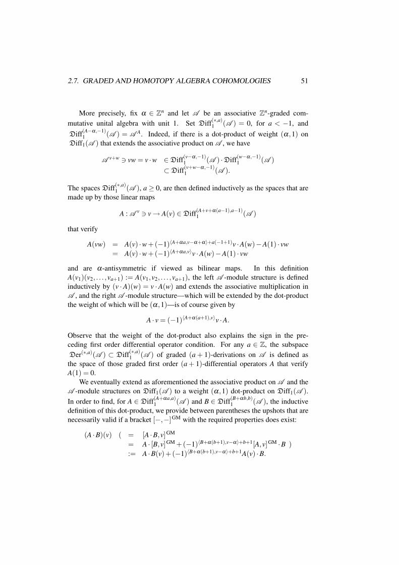
2.7. GRADED AND HOMOTOPY ALGEBRA COHOMOLOGIES 51
More precisely, fix α ∈ Zn and let A be an associative Zn-graded com-mutative unital algebra with unit 1. Set Diff(∗,a)
1 (A ) = 0, for a < −1, andDiff(A−α,−1)
1 (A ) = A A. Indeed, if there is a dot-product of weight (α,1) onDiff1(A ) that extends the associative product on A , we have
A v+w 3 vw = v ·w ∈Diff(v−α,−1)1 (A ) ·Diff(w−α,−1)
1 (A )⊂Diff(v+w−α,−1)
1 (A ).
The spaces Diff(∗,a)1 (A ), a≥ 0, are then defined inductively as the spaces that are
made up by those linear maps
A : A v 3 v→ A(v) ∈Diff(A+v+α(a−1),a−1)1 (A )
that verify
A(vw) = A(v) ·w+(−1)〈A+αa,v−α+α〉+a(−1+1)v ·A(w)−A(1) · vw= A(v) ·w+(−1)〈A+αa,v〉v ·A(w)−A(1) · vw
and are α-antisymmetric if viewed as bilinear maps. In this definitionA(v1)(v2, . . . ,va+1) := A(v1,v2, . . . ,va+1), the left A -module structure is definedinductively by (v ·A)(w) = v ·A(w) and extends the associative multiplication inA , and the right A -module structure—which will be extended by the dot-productthe weight of which will be (α,1)—is of course given by
A · v = (−1)〈A+α(a+1),v〉v ·A.
Observe that the weight of the dot-product also explains the sign in the pre-ceding first order differential operator condition. For any a ∈ Z, the subspaceDer(∗,a)(A ) ⊂ Diff(∗,a)
1 (A ) of graded (a + 1)-derivations on A is defined asthe space of those graded first order (a + 1)-differential operators A that verifyA(1) = 0.
We eventually extend as aforementioned the associative product on A and theA -module structures on Diff1(A ) to a weight (α,1) dot-product on Diff1(A ).In order to find, for A ∈ Diff(A+αa,a)
1 (A ) and B ∈ Diff(B+αb,b)1 (A ), the inductive
definition of this dot-product, we provide between parentheses the upshots that arenecessarily valid if a bracket [−,−]GM with the required properties does exist:
(A ·B)(v) ( = [A ·B,v]GM
= A · [B,v]GM +(−1)〈B+α(b+1),v−α〉+b+1[A,v]GM ·B ):= A ·B(v)+(−1)〈B+α(b+1),v−α〉+b+1A(v) ·B.

52 CHAPTER 2. LODAY INFINITY CATEGORY
Proposition 13. With respect to the abovedetailed bidegree, the pair (Diff1(A ), ·)is an associative Zn+1-graded commutative unital algebra, · has weight (α,1), andthe pair (Der(A ), ·) is a Zn+1-graded subalgebra.
For the proof of this and the next propositions, we refer the reader to [GM03]and [Kra91].
Let us now come to the construction of the Grabowski-Marmo graded Jacobi(resp. Poisson) bracket [−,−]GM on the graded Jacobi (resp. Poisson) cochainalgebra (Diff1(A ), ·) (resp. (Der(A ), ·)). If such a bracket actually exists, wenecessarily have
[v,w]GM = 0, [A,v]GM = A(v), [v,A]GM =−(−1)〈v−α,A+αa〉+a[A,v]GM, (2.61)
and
[A,B]GM(v) = [[A,B]GM,v]GM
= [A, [B,v]GM]GM +(−1)〈B+αb,v−α〉+b[[A,v]GM,B]GM
= [A,B(v)]GM +(−1)〈B+αb,v−α〉+b[A(v),B]GM.
(2.62)
The bracket defined inductively by Equations (2.61) and (2.62) actually fits, see[GM03] and [Kra91]:
Theorem 10. There is a unique Zn+1-graded Jacobi bracket [−,−]GM of degree(0,0)∈Zn×Z on the associative Zn+1-graded commutative algebra (Diff1(A ), ·)that verifies [A,v]GM = A(v). Moreover, (Der(A ), [−,−]GM, ·) is a Zn+1-gradedPoisson algebra.
Furthermore, see again [GM03] and [Kra91],
Proposition 14. The graded Jacobi (resp. Poisson) structures of degree α ∈Zn onthe associative Zn-graded commutative unital algebra A , are exactly the canon-ical elements of degree (2α,1) of the graded Jacobi (resp. Poisson) algebra(Diff1(A ), [−,−]GM, ·) (resp. (Der(A ), [−,−]GM, ·)).
Note that we constructed the algebras Diff1(A ) and Der(A ) for α fixed inZn, and did not write Diff1;α(A ) and Derα(A ) in order to avoid overcrowdednotations. Of course, the graded algebras of Proposition 14 are exactly the justmentioned algebras.
This result immediately leads to the proper concepts of graded Jacobi andgraded Poisson cohomologies.

2.7. GRADED AND HOMOTOPY ALGEBRA COHOMOLOGIES 53
Definition 14. If π denotes a graded Jacobi (resp. Poisson) structure of weight α ∈Zn on (the usual) algebra A , then the graded Jacobi (resp. Poisson) cohomologyof (A ,π) is the cohomology H Jac
π (A ) (resp. H Poiπ (A )) of the DGLA
(Diff1(A ),∂π = [π,−]GM, [−,−]GM)
(resp.(Der(A ),∂π = [π,−]GM, [−,−]GM)).
Let us also recall, see [GM01] and [GM03], that in the geometric (ungraded)situation, i.e. in the case A =C∞(M), where C∞(M) is the associative commutativeunital algebra of smooth functions of a smooth manifold M, we have
(Der(A ), [−,−]GM, ·) = (Γ(∧
T M), [−,−]SN, ∧)),
where [−,−]SN denotes (up to sign) the Schouten-Nijenhuis bracket, and where∧ is the reversed wedge product. Therefore, the aforedefined graded Poisson co-homology coincides in the geometric case with the usual Poisson cohomology,see [Vai94]. Moreover, it has been shown in [GM03] that the preceding gradedJacobi cohomology coincides for A = C∞(M) with the standard Lichnerowicz-Jacobi cohomology, see [Lic78], i.e. with the cohomology of the subcomplexof 1-differentiable cochains of the Chevalley-Eilenberg complex of the Jacobi-Lie bracket on C∞(M) endowed with the natural representation by derivations ofC∞(M).
Link with the Stem bracket
Equations (2.61) and (2.62) pertaining to uniqueness of [−,−]GM allow to ex-plicitly compute the Grabowski-Marmo bracket and to provide evidence that thisbracket is—in the general graded nongeometric situation—the restriction of thepreviously depicted stem bracket, see Equations (2.41) and (2.42).
Proposition 15. For any fixed α ∈ Zn, any A ∈ Diff(A+αa,a)1 (A ) and any B ∈
Diff(B+αb,b)1 (A ), the Grabowski-Marmo bracket [A,B]GM of A by B is given by
[A,B]GM = A¤B− (−1)〈A+αa,B+αb〉+abB¤A, (2.63)
where A¤B is defined inductively by
v¤w := 0, A¤v := A(v), a≥ 0, v¤A := 0, a≥ 0,

54 CHAPTER 2. LODAY INFINITY CATEGORY
(A¤B)(v) := A¤B(v)+(−1)〈B+αb,v−α〉+bA(v)¤B, a,b≥ 0,
for any v ∈A v, w ∈A w. Further, the explicit form of the square-product ¤ is
(A¤B) (v1, . . . ,va+b+1)= ∑ I∪ J = N(a+b+1)
|I|= b+1, |J|= a
(−1)(I;J)ε↓V (I,J)A(B(VI),VJ), (2.64)
where vi ∈A vi , ↓V =↓ v1⊗ . . .⊗ ↓ va+b+1, and ↓ vi ∈A vi−α .
Proof. The proof of Equation (2.63) is by induction on a + b. If a + b ≤ −1,the claim is obviously true, see Equation (2.61). Assume now that it holds true fora + b ≤ k− 1, k ≥ 0, and show that it is still valid for a + b = k. We have, seeEquation (2.62),
[A,B]GM(v) = [A,B(v)]GM +(−1)〈B+αb,v−α〉+b[A(v),B]GM
= A¤B(v)− (−1)〈A+αa,B+v+α(b−1)〉+a(b−1)B(v)¤A+(−1)〈B+αb,v−α〉+bA(v)¤B−(−1)〈B+αb,v−α〉+b+〈A+v+α(a−1),B+αb〉+(a−1)bB¤A(v)
= (A¤B)(v)− (−1)〈A+αa,B+αb〉+ab(B¤A)(v).
In order to determine the explicit form (2.64) of ¤, we proceed again by induc-tion. The announced upshot is clear for a =−1 or b =−1, hence, in particular fora+b≤−1. Let us now assume that it is valid for a+b≤ k−1, k≥ 0, and examinethe case a+b = k. As already pointed out, if a =−1 or b =−1, our conjecture is

2.7. GRADED AND HOMOTOPY ALGEBRA COHOMOLOGIES 55
verified. Otherwise, a,b≥ 0, and, if we set V ′′ = v2⊗ . . .⊗ va+b+1, we obtain
(A¤B)(v1,v2, . . . ,va+b+1)= (A¤B(v1))(v2, . . . ,va+b+1)
+(−1)〈B+αb,v1−α〉+b(A(v1)¤B)(v2, . . . ,va+b+1)= ∑ I∪ J = 2, . . . ,a+b+1
|I|= b, |J|= a
(−1)(I;J)ε↓V ′′(I,J)A(B(v1,V ′′I ),V ′′
J )
+(−1)〈B+αb,v1−α〉+b
∑ I∪ J = 2, . . . ,a+b+1|I|= b+1, |J|= a−1
(−1)(I;J)ε↓V ′′(I,J)A(v1,B(V ′′I ),V ′′
J )
= ∑ . . .
+(−1)〈B+αb,v1−α〉+b+1+〈B+V ′′I −α,v1−α〉
∑ I∪ J = 2, . . . ,a+b+1|I|= b+1, |J|= a−1
(−1)(I;J)ε↓V ′′(I,J)A(B(V ′′I ),v1,V ′′
J )
= ∑ . . .
+(−1)b+1+〈V ′′I −α(b+1),v1−α〉
∑ I∪ J = 2, . . . ,a+b+1|I|= b+1, |J|= a−1
(−1)(I;J)ε↓V ′′(I,J)A(B(V ′′I ),v1,V ′′
J ).
Remark now that in the final result for which we look, I and J are two unshufflesthat form a partition of N(a+b+1), so that 1 is either the first element of I or of J .The first term ∑ . . . (resp. second term (−1)... ∑ . . .) of the RHS of the last equation,corresponds exactly to the first (resp. second) possibility. Indeed,
(−1)(I;J)ε↓V ′′(I,J) = (−1)(I ;J )ε↓V (I ,J )
(resp.
(−1)b+1+〈V ′′I −α(b+1),v1−α〉(−1)(I;J)ε↓V ′′(I,J) = (−1)(I ;J )ε↓V (I ,J )),
which completes the proof.
We now explain in which sense the Grabowski-Marmo bracket coincides withthe stem bracket, which thus governs not only the graded Loday and Lie coho-mologies, but also the graded Poisson and Jacobi cohomologies.
Remark 8. The bracket [−,−]G M on Diff1(A ), which is defined for A ∈Diff(A+αa,a)
1 (A ) and B ∈Diff(B+αb,b)1 (A ) by
[A,B]G M =−(−1)ab[A,B]GM, (2.65)

56 CHAPTER 2. LODAY INFINITY CATEGORY
is clearly a Zn+1-graded Lie bracket on the graded Jacobi and Poisson cochainspaces, which admits these graded algebraic structures as canonical elements.Therefore, the bracket [−,−]G M may also be used to define and compute thegraded Jacobi and Poisson cohomologies.
In the following, we denote by ↓ A the vector space A endowed with thegradation (↓A )γ = A γ+α . Set now
A(A ) =⊕
(A,a)∈Zn×ZA(A+αa,a)(A )
resp. A(↓A ) =
⊕
(A,a)∈Zn×ZA(A+αa,a)(↓A )
,
(2.66)
where A(A+αa,a)(A ) (resp. A(A+αa,a)(↓A )) denotes as usually the space of multi-linear maps A : A ×(a+1) → A (resp. A : (↓ A )×(a+1) →↓ A ) that have weight A(resp. A+αa), i.e.
A : A β1 × . . .×A βa+1 →A A+β1+...+βa+1
(resp.A : (↓A )β1 × . . .× (↓A )βa+1 → (↓A )A+αa+β1+...+βa+1),
and that are further α-antisymmetric (resp. antisymmetric in the usual sense), i.e.
A(. . .v,w . . .) =−(−1)〈v+α,w+α〉A(. . .w,v . . .)
(resp.A(. . . v, w . . .) =−(−1)〈v,w〉A(. . . w, v . . .)).
Obviously, the map ∼: A→ A, with A defined from A by
A(v1, . . . , va+1) =↓ A(↑ v1, . . . ,↑ va+1),
is a graded vector space isomorphism, the inverse of which is v: A→ A,
A(v1, . . . ,va+1) =↑ A(↓ v1, . . . ,↓ va+1).
The graded vector space isomorphism ∼ pulls of course the Nijenhuis-Richardsongraded Lie bracket [−,−]NR on the usual space A(↓ A ), associated with the Zn-graded vector space ↓A , back to a graded Lie bracket
[−,−]N R =v[∼−,∼−]NR =:∼∗[−,−]NR =∼∗[−,−]⊗|A(↓A )
on A(A ).

2.7. GRADED AND HOMOTOPY ALGEBRA COHOMOLOGIES 57
Theorem 11. If π denotes a graded Jacobi (resp. Poisson) structure of weightα ∈ Zn on (the usual) algebra A , the graded Jacobi (resp. Poisson) cohomologyof (A ,π) is the cohomology of the DGLA
(Diff1(A ), [−,−]G M ,∂π = [π,−]G M )
(resp.(Der(A ), [−,−]G M ,∂π = [π,−]G M )),
where [−,−]G M is the restriction of ∼∗ [−,−]⊗|A(↓A ) to Diff1(A ) (resp.Der(A )), i.e. of the Nijenhuis-Richardson bracket or the (restriction of the) stem
bracket read through the canonical isomorphism ∼.
Proof. We need only check that on Diff1(A ) the bracket [−,−]G M is thepullback [−,−]N R by ∼ of the Nijenhuis-Richardson bracket [−,−]NR on A(↓A ). For A ∈ Diff(A+αa,a)
1 (A ) and B ∈ Diff(B+αb,b)1 (A ), this pullback reads, see
Equations (2.17) and (2.66),
[A,B]N R =v iAB− (−1)〈A+αa,B+αb〉+ab v iBA,
where
(v iBA)(VN(a+b+1))
= (−1)〈A+αa,B+αb〉∑ I∪ J = N(a+b+1)
|I|= b+1, |J|= a
(−1)(I;J)ε↓V (I,J) ↑ A(↓↑ B(↓VI),↓VJ)
= (−1)〈A+αa,B+αb〉∑ I∪ J = N(a+b+1)
|I|= b+1, |J|= a
(−1)(I;J)ε↓V (I,J)A(B(VI),VJ)
= (−1)〈A+αa,B+αb〉(A¤B)(VN(a+b+1)).
It follows that
[A,B]N R = (−1)〈A+αa,B+αb〉B¤A− (−1)abA¤B = [A,B]G M ,
see Equations (2.65) and (2.63).
Finally:
Corollary 2. The stem bracket [−,−]⊗ is, up to reading through a canonical iso-morphism, a graded Lie bracket on the spaces of graded Loday, graded Lie, gradedPoisson, and graded Jacobi cochains, for which the corresponding algebraic struc-tures are canonical elements, and that thus encodes the graded cohomologies of allthese structures.

58 CHAPTER 2. LODAY INFINITY CATEGORY
2.7.3 Strongly homotopy and graded p-ary Loday cohomologies
Since LodQ∞ structures on a Zn-graded vector space V , Q ∈ Zn, 〈Q,Q〉 odd, are the
degree Q canonical elements π of the Zn-graded Lie algebra (C(V ), [−,−]⊗), wehave the natural
Definition 15. The cohomology of a Loday infinity algebra (V,π) is the cohomol-ogy of the DGLA (C(V ), [−,−]⊗, [π,−]⊗), where the coboundary operator is, forany ρ ∈Cρ(V ), explicitly given by
[π,ρ]⊗ = ∑q≥1 ∑s+t=q+1(−1)1+(s−1)〈e1,ρ〉[πs,ρt ]⊗
(and Equations (2.41) and (2.42)).
The reader might have noticed that our definition should contain the definitionof graded Loday algebra cohomology, which is a Zn+1-GLA, see Theorem 7,whereas the Loday infinity algebra cohomology is only a Zn-GLA. The followingremarks explain inter alia how the Zn+1-gradation appears in the special case ofp-ary (and in particular binary) brackets.
1. We first examine the case π = πp, p ∈ 2,4,6, . . ., where all but one struc-ture maps vanish. If the odd degree Q ∈ Zn of π is chosen to be equal to (p−1)e1,we have
π = πp ∈M(0,p−1)(V ), [πp,πp]⊗ = 0, p even. (2.67)
Let us recall that essentially two p-ary extensions of the Jacobi identity havebeen investigated during the last decades by mathematicians and physicists—mainly in the skew-symmetric setting. If [−,−, . . . ,−] denotes an p-linearbracket on V , the first is the generalization, which requires that the adjoint action[v1,v2, . . . ,vp−1,−] be a derivation for the p-ary bracket [w1,w2, . . . ,wp], see e.g.[Fil85], and leads to Nambu-Lie or, in the nonantisymmetric context, to Nambu-Loday structures, see [Nam73]. The second has been suggested by P. Michorand A. Vinogradov, see [MV97], and has been further studied in [VV98] andin [VV01]. We refer to this last p-ary extension as p-ary Lie or p-ary Lodaystructure. An p-ary Zn-graded Lie structure on a Zn-graded vector space V is amap Pp ∈ A(0,p−1)(V ), such that iPpPp = 0, where i is the interior product definedin Theorem 2, or, if p is even, equivalently, such that [Pp,Pp]NR = 0. Moreover,the cohomology of an p-ary Lie algebra (V,Pp) is the cohomology of the DGLA(A(V ), [−,−]NR, [Pp,−]NR), see [MV97].
Analogously, we call the above structure π = πp, see Equation (2.67), an p-aryZn-graded Loday structure on V . The cohomology of such a structure should

2.7. GRADED AND HOMOTOPY ALGEBRA COHOMOLOGIES 59
be— and has been defined in the case p = 2 (roughly) as—the cohomology of theDGLA (Mr(V ), [−,−]⊗, [πp,−]⊗).
In the following, we show why the cohomology space of π = πp, viewed asdegree Q = (p−1)e1 Loday infinity structure, coincides with the just guessed co-homology space of π = πp, viewed as p-ary Zn-graded Loday structure.
Let us first mention that in the case of noninfinity algebras, it is conventionalto substitute in cochain space C(V ) a direct sum for the direct product, so that
C(V ) =⊕
s∈N∗
⊕
Q∈Zn
M(Q−(s−1)e1,s−1)(V ) =⊕
s∈N∗Ms−1(V ) = Mr(V ).
Hence, C(V ) coincides with vector space Mr(V ); further C(V) gets bigraded, butits bigrading is shifted with respect to the usual bigradation
Mr(V ) =⊕
s∈N∗
⊕
Q∈Zn
M(Q,s−1)(V )
of Mr(V ).It is now easy to see that the cohomology spaces of
(C(V ), [−,−]⊗, [πp,−]⊗) and (Mr(V ), [−,−]⊗, [πp,−]⊗)
coincide. Indeed, if π is a LodQ∞ structure on V (and in particular in our case π = πp)
and if ρt ∈M(ρ−(t−1)e1,t−1)(V ), we have
[π,ρt ]⊗ = ∑q≥1
(−1)1+(q−t)〈e1,ρ〉[πq−t+1,ρt ]⊗ ∈ ∏q≥1
M(Q+ρ−(q−1)e1,q−1)(V ), (2.68)
so that, in the case π = πp, Q = (p− 1)e1, where necessarily q = t + p− 1, theweight of cohomology operator [πp,−]⊗ with respect to the first mentioned bi-grading is ((p− 1)e1, p− 1). On the other hand, since πp ∈ M(0,p−1)(V ), it isclear that the weight of cohomology operator [πp,−]⊗ with respect to the secondbigradation is (0, p−1). It follows that the cohomology spaces of (C(V ), [πp,−]⊗)and (Mr(V ), [πp,−]⊗), say H and H, are both Zn+1-graded. Space H(ρ+(t−1)e1,t−1)
(resp. H(ρ ,t−1)) is encoded in the cocycle equation
[πp,ρt ]⊗ = 0⇔ [πp,ρt ]⊗ = 0, where ρt ∈M(ρ ,t−1)(V )
(resp.[πp,ρt ]⊗ = 0, ρt ∈M(ρ ,t−1)(V )),

60 CHAPTER 2. LODAY INFINITY CATEGORY
and in the coboundary equation, which reads, as easily understood,
ρt = [πp,τ]⊗ = [πp,±τ]⊗, τ ∈M(ρ ,t−p)(V )
(resp.ρt = [πp,τ ]⊗, τ ∈M(ρ,t−p)(V )),
for any cocycle ρt . This observation obviously entails that
H(ρ+(t−1)e1,t−1) = H(ρ ,t−1).
Eventually, as announced, the cohomology spaces H and H coincide, and theirnatural GLA structures, which are induced by [−,−]⊗ and [−,−]⊗, are Zn- andZn+1-graded respectively.
For p = 2, we of course recover the abovedefined cohomology space of agraded Loday algebra.
2. If π is not a sequence of all but one vanishing elements, Equation (2.68) im-plies that the Loday infinity coboundary operator [π,−]⊗ maps M(ρ−(t−1)e1,t−1)(V )into ∏q≥1 M(Q+ρ−(q−1)e1,q−1)(V ), so that the Loday infinity cohomology is not Z-graded. Nevertheless, if we consider the (decreasing) filtration
Ck(V ) =⊕
R∈Zn∏s≥k
M(R−(s−1)e1,s−1)(V ), k ≥ 1,
and if ρ = ∑R ∑t≥k ρR,t ∈Ck(V ), we get
[π,ρ]⊗ = ∑R ∑q≥1 ∑s+t=q+1(−1)1+(s−1)〈e1,R〉[πs,ρR,t ]⊗
∈⊕R∈Zn ∏q≥k M(Q+R−(q−1)e1,q−1)(V ).
Indeed, as k ≤ t, we have q ≤ k− 1 ⇒ q ≤ t− 1 ⇔ s = q− t + 1 ≤ 0, so that thesum over s, t vanishes for these q. The observation yields
[π,Ck(V )]⊗ ⊂Ck(V ).
Eventually, differential space (C(V ), [π,−]⊗) is a differential filtered module andthe theory of spectral sequences may be applied.

Chapter 3
Lie infinity algebras andDeformation Quantization
This Chapter intends to analyze the role of L∞ algebras in deformation theory andto review Kontsevich’s formality Theorem together with his star product formula.
We will make use of the same notations employed previously in Chapter 2.
3.1 Lie infinity algebras and their morphisms
Let V be a Zn-graded vector space, and consider the Zn-graded vector subspace
C (V ) =⊕
Q∈Zn
C Q(V ) =⊕
Q∈Zn∏s≥1
A(Q−(s−1)e1,s−1)(V )
of C(V ), which is made up by finite sums of sequences of Zn-graded skew-symmetric multilinear maps on V , see Equation (2.16). Let [−,−]NR be the re-striction of the Zn-graded Lie stem bracket [−,−]⊗, introduced in Equation (2.40),to C (V ). The bracket [−,−]NR is obviously a Zn-graded Lie bracket on C (V ) and,for any graded antisymmetric sequences π,ρ , we have
[π,ρ]NR = ∑q≥1
∑s+t=q+1
(−1)1+(s−1)〈e1,ρ〉[πs,ρt ]NR,
since [−,−]⊗ coincides with [−,−]NR on A(V ).
61

62 CHAPTER 3. L∞ ALGEBRAS AND DEFORMATION QUANTIZATION
If the structure maps of a Lod∞ algebra (V,π) are Zn-graded skew-symmetric,we recover the notion of Lie infinity (L∞ for short) algebra. One easily ascertainsthat the definition of L∞ algebras given in [LS93] coincides with the following
Definition 16. A given pair (V,π), made up by a Zn-graded vector space V and asequence
π ∈ C e1(V ) = ∏s≥1
A((2−s)e1,s−1)(V ),
is an L∞ algebra if and only if [π,π]NR = 0, i.e. if and only if
∑s+t=p
(−1)s[πs,πt ]NR = 0, ∀p≥ 2. (3.1)
We denote by L∞(V ) the set of L∞ structures on V .
Example 3. An L∞ algebra (V,π) reduces to a DGLA, if all structure maps πs
vanish, except π1 and π2.
Since L∞ structures on V are the degree e1 canonical elements of the Zn-gradedLie algebra (C (V ), [−,−]NR), the cohomology of an L∞ structure π on V is thecohomology of the DGLA (C (V ), [−,−]NR, [π,−]NR). This cohomology has beenstudied in [Pen01] and used in [FP02].
Remark 9. Replacing in (3.1) bracket [−,−]NR with bracket [−,−]G, see Equa-tion (2.15), we recover the concept of A∞ algebra [LS93] which is the homotopyalgebra that generalizes associative algebras.
We have seen that L∞ structures on V are particular Lod∞ structures on thenonshifted side. However, on the shifted side, L∞ structures on V may alsobe viewed as odd codifferentials, but of a different coalgebra, namely of thecoassociative symmetric tensor coalgebra of ↓ V . In the following, we recall thiscoalgebraic description, but skip most of the proofs.
Remember that the (reduced) symmetric associative tensor algebra S(V ) is thequotient of the (reduced) associative tensor algebra T (V ) by the ideal generatedby the elements of the form v1⊗ v2− (−1)〈v1,v2〉v2⊗ v1. The induced product onS(V ) will be denoted by ∨. The algebra S(V ) inherits both, the Z-gradation andthe Zn-gradation. In the sequel, we consider S(V ) as a Zn-graded vector space.
Proposition 16. The coproduct
∆S : S(V )→ S(V )⊗
S(V ),

3.1. LIE INFINITY ALGEBRAS AND THEIR MORPHISMS 63
defined by
∆S(v1∨ . . .∨ vp) = ∑I∪J=N(p)
I,J 6= /0
εV (I;J) VI⊗
VJ (v` ∈V v` , p≥ 1), (3.2)
provides a graded coassociative coalgebra structure on S(V ). Here, VI = vi1∨ . . .∨vi|I| , for any unshuffle I.
In the following theorem, we characterize the space of coderivationsCoDer(S(V )) of the coalgebra (S(V ),∆S).
Theorem 12. A homogenous coderivation QS of weight QS ∈ Zn of the coalgebra(S(V ),∆S) is uniquely determined by its corestriction maps
QSp : SpV → S(V )
QS
−→ S(V )pr−→V,
via the equation
QS(v1∨ . . .∨ vp) = ∑I∪J=N(p)
I 6= /0
εV (I;J)QS|I|(VI)∨VJ. (3.3)
If S (V ) denotes the Zn+1-graded vector subspace of M(V ) made up by theZn-graded symmetric multilinear maps
A(. . . ,vi,vi+1, . . .) = (−1)〈vi,vi+1〉A(. . . ,vi+1,vi, . . .), (3.4)
then, clearly, the sequence of corestriction maps (QS1,Q
S2, . . .) of a coderivation QS
of weight QS ∈ Zn, is an element of the direct product space ∏s≥1 S (QS,s−1)(V ),and the preceding proposition implies that the mapping
ψS : CoDerQS(S(V )) 3 QS → (QS
1,QS2, . . .) ∈∏
s≥1S (QS,s−1)(V )
is a vector space isomorphism. Furthermore, since, for any ρ ∈ Zn, the maps
A(ρ−(s−1)e1,s−1)(V ) 3 A→ (−1)s(s−1)
2 ↓ A ↑∨s∈S (ρ ,s−1)(↓V ), (3.5)
where s ≥ 1 and where notations are self-explaining, are vector space isomor-phisms, their composition with (ψS)−1 provides the isomorphisms
φ Sρ : C ρ(V ) = ∏
s≥1A(ρ−(s−1)e1,s−1)(V )→ CoDer ρ(S(↓V )).

64 CHAPTER 3. L∞ ALGEBRAS AND DEFORMATION QUANTIZATION
Proposition 17. Let [−,−]S be the Zn-graded Lie bracket of the space of coderiva-tions of (S(↓V ),∆S). Then, the aforementioned Zn-graded Lie bracket [−,−]NR onC (V ) is given by
[π,ρ]NR = (φ Sπ+ρ)−1[φ S
π (π),φ Sρ (ρ)]S, π ∈ C π(V ),ρ ∈ C ρ(V ).
Consequently,
Proposition 18. A sequence π ∈ C e1(V ) is an L∞ structure on the Zn-graded vec-tor space V if and only if the weight e1 coderivation QS := φ S
e1(π) of (S(↓ V ),∆S)
is a codifferential.
We now introduce the notion of L∞ morphisms.
Definition 17. Let (V,QS) and (V ′,Q′S) be two L∞ algebras. An L∞ morphismfrom (V,QS) to (V ′,Q′S) is a coalgebra cohomomorphism
F S : (S(↓V ),∆S)−→ (S(↓V ′),∆S),
which intertwines the codifferentials QS and Q′S, i.e. verifies
Q′SF S = F SQS. (3.6)
Proposition 19. Let V and V ′ be two Zn-graded vector spaces. A coalgebra coho-momorphism
F S : (S(V ),∆S)−→ (S(V ′),∆S)
is uniquely determined by its corestriction maps
F Sp : SpV → S(V ) F S−−→ S(V ′)
pr−→V ′, p≥ 1,
via the equation
F S(v1∨ . . .∨ vp) =p
∑s=1
1s! ∑
I1∪...∪Is=N(p)
I1,...,Is 6= /0
εV (I1; . . . ; Is)F S|I1|(VI1)∨ . . .∨F S
|Is|(VIs),
(3.7)where v` ∈V v` , for all ` ∈ 1, . . . , p.
Since a coalgebra cohomomorphism F S : (S(↓ V ),∆S) → (S(↓ V ′),∆S) “is”of course a sequence f S = ( f S
1 , f S2 , . . .) of weight (1− s)e1, Zn−graded skew-
symmetric multilinear maps f Ss : V×s → V ′ that are defined by f S
s =↑ F Ss ↓∨s,
we obtain the following equivalent interpretation of L∞ morphisms:

3.2. GENERALIZED MAURER CARTAN EQUATION 65
Proposition 20. Let (V,πS) and (V ′,π ′S) be two L∞ algebras. An L∞ morphismf S : (V,πS)→ (V ′,π ′S) is a sequence of Zn−graded skew-symmetric weight (1−s)e1 multilinear maps f S
s , s ≥ 1, which satisfy conditions (2.52) (with π ′S, f S, andπS substituted for π ′, f , and π respectively).
It follows that the category L∞ is a subcategory of the category Lod∞. Letus recall that a subcategory of a category C is a category whose objects andmorphisms are objects and morphisms in C and that has the same composition ofmorphisms and the same unit morphisms.
In the following, any DGLA (V,d,−,−) we consider has a weight e1 differ-ential d, so that hence V can be seen as an L∞ algebra.
3.2 Generalized Maurer Cartan Equation
In this Section, we recall the notion of Maurer Cartan elements of L∞ algebras andprove that this notion is preserved under the action of L∞ morphisms.
Definition 18. Let (V,d,−,−) be a DGLA. A Maurer Cartan element w of V isa degree e1 element satisfying the Maurer Cartan equation (MCE for short)
d w− 12w,w= 0. (3.8)
The MCE can naturally be generalized to an L∞ algebra (V,QS) ∼ (V,π) byconsidering the equation
∑s≥11s! Q
Ss (↓ w, . . . ,↓ w) = 0, (3.9)
or, equivalently,∑s≥1
1s!(−1)
s(s−1)2 πs(w, . . . ,w) = 0 (3.10)
for any w ∈ V e1 , because if the L∞ algebra (V,π) is a DGLA, i.e. π1 = d,π2 = −,− and π3 = π4 = . . . = 0, one recognizes the ordinary MCE (3.8).
The reader may have noticed that in equation (3.9) we encounter a convergenceproblem, because this equation yields an infinite sum in the case of infinitely manynonzero QS
` . We apply the standard solution to this problem:Let K be a finite dimensional local K−algebra (commutative with unit), with anilpotent maximal ideal m, i.e. there exists N ∈ N such that mN = 0. If (V,QS) isan L∞ algebra, then Vm := V ⊗Km has an L∞ structure given by the codifferential

66 CHAPTER 3. L∞ ALGEBRAS AND DEFORMATION QUANTIZATION
Qm of corestriction maps QSm`, ` ≥ 1, which are the K −multilinear natural
extensions of the corestriction maps QS` . Hence, for an element w ∈ V e1 ⊗K m,
obviously Q`(↓ w, . . . ,↓ w) = 0 if `≥ N, and so equation (3.9) makes sense.
From now on, we shall assume that any L∞ algebra (V,QS) we consider, hasbeen tensored with a nilpotent maximal ideal m of a finite dimensional local ringK , and we denote the result by the same (V,QS).
Definition 19. Let (V,QS) be a nilpotent L∞ algebra. A Maurer Cartan elementw of V is a degree e1 element satisfying the generalized Maurer Cartan equation(GMCE)
QS∗(↓ w) = ∑s≥11s! Q
Ss (↓ w, . . . ,↓ w) = 0.
Remark 10. Let us mention that a modification of the Definition 16 of L∞ algebrasvia the transformation πs 7→ πs := (−1)
s(s−1)2 πs allows to write all terms of the equa-
tion (3.10) with +1−signs rather than the signs (−1)s(s−1)
2 . With this modification,the L∞ structure conditions (3.1) become
∑s+t=p(−1)s(p+1)[πs, πt ]NR = 0, ∀p≥ 2.
Henceforth, we keep the convention of signs fixed in Definition 16.
The upcoming Proposition provides an equivalent formulation for the GMCE.Given an element v ∈V , let us denote by ev the exponential
ev = ∑s≥11s! v∨ . . .∨ v︸ ︷︷ ︸
s
.
Proposition 21. A degree e1 element w of an L∞ algebra (V,QS) is a MaurerCartan element if and only if
QS(e↓w) = 0.
Proof. Applying (3.3), for any v ∈V 0, we have
QS(ev) = ∑i≥11i! Q
S(v∨ . . .∨ v︸ ︷︷ ︸i
)
= ∑i≥11i! ∑i
j=1C ji QS
j(v∨ . . .∨ v︸ ︷︷ ︸j
)∨ v . . .∨ v
= QS∗(v)∨ (ev +1)

3.2. GENERALIZED MAURER CARTAN EQUATION 67
where 1 is defined so that V∨k ∨ 1∨V∨l = V∨k+l for any k, l ≥ 0. As ev + 1 isinvertible (of inverse 1 + e−v), then, when replacing in the previous equality v by↓ w, we get QS(e↓w) = 0 if and only if QS∗(↓ w) = 0.
We shall denote the set of Maurer Cartan elements of an L∞ algebra (V,QS) byMC(V ).
Our next task is to prove that the set MC(V ) of an L∞ algebra (V,QS) is pre-served under the action of L∞ morphisms. To achieve this goal, we need the fol-lowing preliminaries.
Definition 20. An even degree element p of the coalgebra (S(↓V ),∆S) is called agroup-like element if ∆S p = p⊗ p.
Lemma 4. The set of group-like elements of S(↓ V ) is made up by elements ev,where v is any even degree element of ↓V .
Proof. When applying (3.2), we can clearly see that ∆Sev = ev⊗ ev. Hence,ev is a group like element. Conversely, take p ∈ S(↓ V ) as a group-like element.Write p as the sum ∑i≥1 pi, where each pi is an even degree element in Si(↓ V ).The equation ∆S p = p⊗ p implies that
∆S pi = ∑ j+k=i p j⊗ pk (3.11)
for any i ≥ 1. For i = 2, we get ∆S p2 = p1⊗ p1 and so, in view of the definitionof ∆S, p2 = 1
2! p1 ∨ p1. Proceeding by induction, we easily see that pi = 1i!(p1)i.
Therefore, we get p = ep1 .
Proposition 22. Let (V,QS) and (V ′,Q′S) be two L∞ algebras and assume that anL∞ morphism F S : (V,QS)→ (V ′,Q′S) has been defined. If w is a Maurer Cartan
element of (V,QS), then the element
F S∗ (↓ w) := ∑∞s=1
1s! ↑F S
s (↓ w, . . . ,↓ w) (3.12)
is a Maurer Cartan element of (V ′,Q′S).
Proof. Set w′ = F S∗ (↓ w). Observe first that w′ is a e1 degree element of V ′
since ↓ w is of degree zero and the maps F Ss , s ≥ 1, are of weight zero. We now
show that w′ satisfies the generalized Maurer Cartan Equation, or, equivalently, thatQ′S(e↓w′) = 0 (see Proposition 21).Since F S is an L∞ morphism, i.e. F S QS = Q′S F S and since QS(e↓w) = 0, we

68 CHAPTER 3. L∞ ALGEBRAS AND DEFORMATION QUANTIZATION
have Q′S(F S(e↓w)) = 0. By showing that e↓w′ = F S(e↓w), we obtain the proof.Since F S is a coalgebra cohomomorphism and since ∆S(e↓w) = e↓w⊗ e↓w, then
∆SF S(e↓w) = (F S⊗F S)∆S(e↓w) = F S(e↓w)⊗F S(e↓w)
and so F S(e↓w) is a group-like element. According to Lemma 4, F S(e↓w) is there-fore equal to ev′ , where v′ is the projection of F S(e↓w) on ↓V ′. Using (3.7), it canbe easily checked that
v′ = ∑∞s=1
1s!F
Ss (↓ w, . . . ,↓ w) =↓ w′.
3.3 Twisted L∞ algebras and Twisted L∞ quasi-isomorphisms
Referring to the papers [Ye06] and [Dol05], we recall in this Section the twistingprocedure of L∞ algebras and L∞ quasi-isomorphisms by Maurer Cartan elements.
Given an L∞ algebra (V,QS) endowed with a Maurer Cartan element w ∈V e1 ,a new L∞ structure on V is obtained as follows:
Proposition 23. Let (V,QS) be an L∞ algebra equipped with a Maurer Cartanelement w. Define a coderivation QSw on (S(↓V ),∆S) with corestriction maps
QSwp (↓ v1, . . . ,↓ vp) := ∑i≥0
1i! Q
Sp+i(↓ w, . . . ,↓ w,↓ v1, . . . ,↓ vp)
for any v1, . . . ,vp ∈ V and any p ≥ 1. The pair (V,QSw) is an L∞ algebra, calledthe twisted L∞ algebra of (V,QS) by the Maurer Cartan element w.
Proof. Consider the coalgebra map
Q : S(↓V )→ S(↓V )
defined byQ := ϕ−1
w QSϕw
where ϕw is the invertible coalgebra map
ϕw : S(↓V )→ S(↓V ), X 7→ (1+ e↓w)∨X .
It is easily seen that the map Q satisfies Q2 = 0 (because Q is a codifferential)and that its corestriction maps coincide with QSw
p for any p ≥ 1. Hence, in view

3.3. TWISTED L∞ QUASI-ISOMORPHISMS 69
of Theorem 12, if we prove that Q is a coderivation then QSw = Q and we canconclude that the pair (V,QSw) is an L∞ algebra.Let us then show that Q is a coderivation. By application of equation (3.2), a directcomputation shows that for any X ∈ S(↓V ) and any s ∈ Z
∆Sϕsw(X) = (ϕt w⊗ϕsw)∆S(X)+ e↓tw⊗ϕsw(X)+ϕsw(X)⊗ e↓sw. (3.13)
Hence, it follows that
∆S(Q(X)
)= ∆S
(ϕ−1
w(QSϕw (X)
))
=(ϕ−1
w ⊗ϕ−1w
)(∆S
(QSϕw(X)
))
+e↓−w⊗ϕ−1w
(QSϕw (X)
)+ϕ−1
w(QSϕw (X)
)⊗ e↓−w
=(ϕ−1
w ⊗ϕ−1w
)((QS⊗ id+ id⊗QS
)(∆S (ϕw(X))
))
+e↓−w⊗ϕ−1w
(QSϕw (X)
)+ϕ−1
w(QSϕw (X)
)⊗ e↓−w
=(ϕ−1
w ⊗ϕ−1w
)
((QS⊗ id+ id⊗QS
)((ϕw⊗ϕw)∆S (X)+ e↓w⊗ϕw (X)+ϕw (X)⊗ e↓w
))
+e↓−w⊗ϕ−1w
(QSϕw (X)
)+ϕ−1
w(QSϕw (X)
)⊗ e↓−w
=(
QS⊗ id+ id⊗QS)(
∆S (X)),
where in the last equality we use the propriety QS(e↓w) = 0 (w is a Maurer Cartanelement) as well as the following obvious identity
ϕ−1w (e↓w) =−e↓−w.
Example 4. Let (V,QS)∼ (V,π) be an L∞ algebra equipped with a Maurer Cartanelement w. If (V,π) is a DGLA (V,d,−,−), then the twisted DGLA of (V,π) byw is the DGLA (V,d−w,−,−,−).Proposition 24. Let (V,QS) and (V ′,Q′S) be two L∞ algebras and assume that anL∞ quasi-isomorphism F S : (V,QS)→ (V ′,Q′S) has been defined. Set an element
w ∈MC(V ) and let w′ = F S∗ (↓ w) be the element of MC(V ′) as defined in Propo-sition 22. Let (V,QSw) and (V ′,Q′Sw′) be respectively the twisted L∞ algebra of

70 CHAPTER 3. L∞ ALGEBRAS AND DEFORMATION QUANTIZATION
(V,QS) and (V ′,Q′S) by the Maurer Cartan elements w and w′. Then the sequenceof maps
F Sws (↓ v1, . . . ,↓ vp) := ∑i≥0
1i!F
Ss+i(↓ w, . . . ,↓ w,↓ v1, . . . ,↓ vs), s≥ 1 (3.14)
defines an L∞ quasi-morphism F Sw from (V,QSw) to (V ′,Q′Sw′), called the twistedL∞ quasi-morphism of the L∞ quasi-morphism F S by w.
Proof. Set F := ϕ−1w′ F Sϕw. As F S is an L∞ morphism, then FQSw = Q′Sw′F .
By application of equation (3.13), and by using similar reasoning developed in theprevious proof, we see that
∆SF = (F ⊗F )∆S.
Hence, F is an L∞ morphism from (V,QSw) to (V ′,Q′Sw′). Moreover, as thecorestriction maps of F are exactly F Sw
p , p ≥ 1, then F Sw = F is an L∞morphism. By application of spectral sequence arguments it can be shown thatF Sw is an L∞ quasi-isomorphism (i.e. (F Sw
1 )] is an isomorphism between thecorresponding cohomology). We refer the reader to [Dol05].
Dolgushev [Dol05] used this twisting technique in his globalization procedurefor the local Kontsevich’s formality onRd . Chapter 4 will review this construction.We will see next that this technique is also useful for investigating some proprietiesof the Moduli space of L∞ algebras.
3.4 Moduli space of L∞ algebras
Let K[[t]] be the space of polynomials in the parameter t with coefficients in K.
Definition 21. Given an L∞ algebra (V,QS), two elements w0 ∈MC(V ) and w1 ∈MC(V ) are called gauge equivalent if and only if there exists an element u(t) ∈V 0⊗K[[t]] such that
ddt ↓ w(t) = QSw(t)
1 (↓ u(t)) = ∑i≥01i! Q
S1+i(↓ w(t), . . . ,↓ w(t)︸ ︷︷ ︸
i
,↓ u(t)) (3.15)
where w(t) lies in MC(V ⊗K[[t]]) satisfying w(0) = w0 and w(1) = w1.
Here, V ⊗K[[t]] inherits the L∞ structure of V with obvious manner.Clearly, this gauge transformation is an equivalence relation and we can there-
fore define

3.4. MODULI SPACE OF L∞ ALGEBRAS 71
Definition 22. Given an L∞ algebra (V,QS), the set of gauge equivalence classesof MC(V ) is the moduli space
M (V ) := MC(V )/∼,
where ∼ is the gauge equivalence in Definition 21.
A geometric meaning of the gauge equivalence was given in terms of thelanguage of Q−manifold, see [Kon03]; we will not discuss this point further.However, let us explain why the moduli space M (V ) in the sense of L∞ algebrascoincides with the “ordinary” well known moduli space Def(V ) in the sense ofDGLAs.
Let us first recall the definition of the space Def(V ) of any DGLA(V,d,−,−). Just as for the space M (V ), Def(V ) of a given DGLA V is com-posed by the set of Maurer Cartan elements, but modulo the gauge group action.The gauge group of the DGLA V is the group G(V ) = exp(V 0), where the multi-plication is given by the Baker-Campbell-Hausdorff formula:
exp(u) exp(v) = exp(H(u,v)),
whereH(u,v) = u+ v+
12u,v+ . . .
for any u,v ∈V 0. Note that this product is well defined since V is actually V ⊗Kmand m is nilpotent. The group G(V ) acts on V e1 by
exp(u).w = exp(adu)w+∑i≥0(adu)i
(i+1)! du (3.16)
for any u∈V 0 and w∈V e1 . It is quite easy to show that this action preserves the setMC(V ). Indeed, if we assume that d,d = 0 and x,d = d,x = (−1)〈e1,x〉dxfor any x in V 0 or in V 1, then the MCE (3.8) reads
d +w,d +w= 0
and the gauge group action (3.16) can be written as
exp(u).w+d = exp(adu)(w+d).
Moreover, since exp(adu) is a Lie algebra morphism (see Lemma 1), then for anyw ∈MC(V )
d + exp(u).w,d + exp(u).w = exp(adu)(w+d), exp(adu)(w+d)= exp(adu)(w+d,w+d) = 0.

72 CHAPTER 3. L∞ ALGEBRAS AND DEFORMATION QUANTIZATION
Thus, we define the moduli space of the DGLA V as the quotient Def(V ) =MC(V )/G(V ).
Proposition 25. If (V,QS)∼ (V,d,−,−) is a DGLA, then M (V ) = Def(V ).
Proof. Let w0 and w1 be two elements of MC(V ) that are gauge equivalent bymeans of the gauge group action, i.e. there is u ∈ V 0 so that w1 = exp(u).w0. Wewant to show that w0 and w1 are gauge equivalent in the sense of L∞ algebras as inDefinition 21. When taking u = u(t) and w(t) = exp(tu).w0, we get
ddt↓ w(t) =
ddt↓ (exp(ad tu)(w0 +d)−d)
= ↓ u, exp(ad tu)(w0 +d)= ↓ d u+ ↓ u,w(t)=↓ d u− ↓ wt ,u= QS
1(↓ u)+QS2(↓ w(t),↓ u)
where in the last equality we use d =↑ Q1 ↓ and −,− =↑ Q2 ↓∨2—see Propo-sition 18. This proves that a gauge equivalence in the sense of DGLAs implies agauge equivalence in the sense of L∞ algebras.Conversely, suppose now that w0 and w1 are equivalent in the sense of L∞ algebras,i.e. there is u(t) ∈V 0⊗K[[t]] so that
ddt↓ w(t) = QS
1(↓ u(t))+QS2(↓ w(t),↓ u(t)),
where w(t) ∈ MC(V ⊗K[[t]]) satisfies w(0) = w0 and w(1) = w1. As previouslyshown,
ddt
w(t) = d u(t)+u(t),w(t)= u(t),w(t)+d
and so
ddt
(w(t)+d) = u(t),w(t)+d.
It follows that w(t) = exp(adu(t))(w0)− d = exp(u(t)).w0 is a solution for theabove differential equation. Hence w1 = exp(u(1)).w0 and so w0 and w1 are equiv-alent by means of the gauge group action (3.16). We conclude therefore thatDef(V ) = M (V ).
Example 5. The moduli space of a contractible L∞ algebra (V,QS) is trivial. In-deed, since the set of Maurer Cartan elements is
MC(V ) = w ∈V e1 ; QS1(↓ w) = 0

3.4. MODULI SPACE OF L∞ ALGEBRAS 73
and because the cohomology space H(V,QS1) is trivial, there exists u ∈ V 0 so that
QS1(↓ u) =↓ w. As the element w(t) = tw lies in MC(V ⊗K[[t]]), then equation
(3.15) implies that the class of w = w(1) in M (V ) is that of w(0) = 0.
Example 6. Let (V,QS) and (V ′,Q′S) be two L∞ algebras. Consider (V ⊕V ′,QS⊕Q′S) the direct sum L∞ algebra of (V,QS) and (V ′,Q′S), where QS ⊕Q′S is thecodifferential defined by
QS⊕Q′S |S(↓V ) = QS, QS⊕Q′S |S(↓V ′) = Q′S and QS⊕Q′S |S(↓V )∨S(↓V ′) = 0.
Then
M (V ⊕V ′)∼= M (V )×M (V ′).
Indeed, by definition of the direct sum L∞ algebra, it is clear that MC(V ⊕V ′) ∼=MC(V )×MC(V ′). Moreover, this factorization is preserved by the gauge equiv-alence because the twisted L∞ algebra of the L∞ algebra (V ⊕V ′,QS ⊕Q′S) byan element w + w′ ∈ MC(V ⊕V ′) is nothing else than the direct sum L∞ algebra(V ⊕V ′,QSw ⊕Q′Sw′) of the twisted L∞ algebras (V,QSw) and (V ′,Q′Sw′). Thisproves the claim.
Subsequently, we shall show that the gauge equivalence is preserved under theaction of L∞ morphisms.
According to Proposition 22, any L∞ morphism F S : (V,QS) → (V ′,Q′S) in-duces a well defined map F S∗ : MC(V ) → MC(V ′) which assigns the elementF S∗ (↓ w) ∈MC(V ′) given in (3.12) to any element w ∈MC(V ). Moreover
Proposition 26. The map F S∗ descends to the quotients by the gauge equivalence,providing a well defined map MF S∗ : M (V )→M (V ′) between the correspondingmoduli spaces.
This result raises from
Lemma 5. Set w0,w1 ∈MC(V ). If w0 ∼ w1, then F S∗ (↓ w0)∼F S∗ (↓ w1).
Proof. Assume that w1 ∼ w2 and consider an element w(t) ∈ MC(V ⊗K[[t]])

74 CHAPTER 3. L∞ ALGEBRAS AND DEFORMATION QUANTIZATION
and an element u(t) ∈V 0⊗K[[t]] as in Definition 21. It is easily seen that
ddt↓F S
∗ (↓ w(t)) = ∑s≥1
1s!
ddt
F Ss (↓ w(t), . . . ,↓ w(t))
= ∑s≥1
1(s−1)!
F Ss
(ddt↓ w(t),↓ w(t) . . . ,↓ w(t)
)
= ∑s≥0
1s!
F S1+s
(QSw(t)
1 (↓ u(t)),↓ w(t), . . . ,↓ w(t))
(∗)= F
Sw(t)1
(QSw(t)
1 (↓ u(t)))
,
where at (∗) we use equation (3.14). Moreover, from Proposition 24, we knowthat F Sw(t) is an L∞ morphism from the twisted L∞ algebra (V ⊗K[[t]],QSw(t)) tothe twisted L∞ algebra (V ′⊗K[[t]],Q′Sw′(t)), where w′(t) = F S∗ (↓ w(t)). Thus, itfollows that F
Sw(t)1 QSw(t)
1 = QSw′(t)1 F
Sw(t)1 and so
ddt↓F S
∗ (↓ w(t)) = QSw′(t)1
(F
Sw(t)1 (↓ u(t))
).
This entails that F S∗ (↓ w0)∼F S∗ (↓ w1) and proves the Proposition.
With this premise, we are finally prepared to prove the main Theorem and shallalso later explain its crucial role for deformation theory.
Theorem 13. Let (V,QS) and (V ′,Q′S) be two L∞ algebras and assume that an L∞quasi-morphism F S : (V,QS)→ (V ′,Q′S) has been defined. The mapping MF S∗ :M (V )→M (V ′) is an isomorphism.
Proof. By application of the minimal model Theorem, V (resp. V ′) is L∞isomorphic to the direct sum Vm ⊕Vc (resp. V ′
m ⊕V ′c) of a minimal L∞ alge-
bra Vm (resp. V ′m) and a contractible L∞ algebra Vc (resp. V ′
c). Composing theaforementioned two L∞ isomorphisms with the considered L∞ quasi-morphismF S : (V,QS)→ (V ′,Q′S), we get an L∞ quasi-morphism from Vm⊕Vc to V ′
m⊕V ′c ,
which will also be denoted by F S. The composition of the following L∞ quasi-morphisms
Vmιm→Vm⊕Vc
F S→ V ′m⊕V ′
cP′m³ V ′
m,
provides an L∞ quasi-morphism F Sm : Vm →V ′m, which is actually an L∞ isomor-
phism (see the proof of Theorem 8). Thus, the induced composition
M (Vm)M ιm∗→ M (Vm)×M (Vc)
MF S∗→ M (V ′m)×M (V ′
c)M Pm∗³ M (V ′
m)

3.4. MODULI SPACE OF L∞ ALGEBRAS 75
is the induced isomorphism MF Sm : M (Vm) → M (V ′m). Moreover, as seen in
Example 5, both M (Vc) and M (V ′c) are trivial. Thus, M ιm∗ and M Pm∗ are two
isomorphisms. This entails that MF S∗ is an isomorphism and completes the proofof the Theorem.
3.4.1 Application: Moduli space of a canonical element
Let us consider a GLA (g,−,−) endowed with a e1 degree canonical element π .Remember that the triple (g,∂π ,−,−) is a DGLA with ∂π being the Hamiltoniandifferential π,−, and that this DGLA structure induces a formal DGLA (g⊗νK[[ν ]],∂π ,−,−) in an obvious manner. Remember also that a formal series
πν = π +∑i≥1 ν iπi ∈ ge1 ⊗K[[ν ]]
is a formal deformation of π if and only if
∂π(πp)+ 12 ∑i+ j=pπi,π j= 0, ∀p≥ 1,
i.e. if and only if∂πCπ + 1
2Cπ ,Cπ= 0, (3.17)
where Cπ is the formal series
Cπ := ∑i≥1 ν iπi ∈ ge1 ⊗νK[[ν ]].
When modifying the formal DGLA structure of g⊗νK[[ν ]] by setting
−,−− :=−1×−,−, (3.18)
then, in view of equation (3.17), Cπ is a Maurer Cartan element of the formalDGLA g− := (g⊗νK[[ν ]],∂π ,−,−−).
This allows concluding that the set of Maurer Cartan elements MC(g−) of theformal DGLA g− encodes all formal deformations of π .
Let us now consider two equivalent formal deformations π ′ν and πν of π in thesense of Definition 5, i.e. there is a formal series χν ∈ g0⊗K[[ν ]] so that
π ′ν = exp(ad χν) πν = exp(ad− ξν) πν , (3.19)
where ξν = −χν and ad− ξν = ξν ,−−. When writing π ′ν = π +C′π , it follows,as seen previously, that C′π ∈ MC(g−) and, moreover, C′π satisfies
C′π = exp(ad− ξν)Cπ +∑i≥0(ad− ξν )i
(i+1)! ∂πξν .

76 CHAPTER 3. L∞ ALGEBRAS AND DEFORMATION QUANTIZATION
This defines an equivalence between Maurer Cartan elements of MC(g−).This equivalence is clearly similar to the gauge equivalence defined in equa-tion (3.16) with the only difference being that the Lie algebra νg0[[ν ]] is notnilpotent. Nevertheless, we can formally define the gauge group as the setG(g−) := exp(g0 ⊗ νK[[ν ]]) and introduce a well defined product taking (for-mally) the Baker-Campbell-Hausdorff formula. Therefore, the moduli space ofthe formal DGLA g− is the quotient Def(g−) := MC(g−)/G(g−) made up by theset of all classes of formal deformations of the canonical element π .
If g is the GLA (Mr(V ), [−,−]⊗) (resp. (M(V ), [−,−]G), (A(V ), [−,−]NR),(Diff1(V ), [−,−]NR), (Der(V ), [−,−]SN)) and π is a graded Loday structure(resp. a graded associative structure, a graded Lie structure, a 0−weight gradedJacobi structure, a 0−weight graded Poisson structure) on V , then Def(g−)represents the classes of all formal deformations of π , where g− is the for-mal DGLA (g ⊗ νK[[ν ]],∂π , [−,−]⊗−) (resp. (M(V ),∂π , [−,−]G−),. . .) with[−,−]⊗− =−1× [−,−]⊗ ( resp. [−,−]G− =−1× [−,−]G, . . .).As it is easily understood from the above discussion, we modify the original GLAby multiplying the bracket by −1 in order to get the right sign in the MaurerCartan Equation (3.8).
We have now seen two points of view on how to control formal deformations:firstly, the cohomological approach given in Section 2.2, and secondly, in termsof the corresponding modulo space. The second point of view has been revealedas being more efficient for building equivalence between two different deforma-tion problems; more particularly, if the corresponding formal DGLAs of the twodeformation problems are quasi-isomorphic as L∞ algebras then, by application ofTheorem 13, the corresponding moduli spaces of the two (formal) induced DGLAsare isomorphic. This was one of the main ingredients used by Kontsevich to builda one-to-one correspondence between formal Poisson structures and star productson Poisson manifolds, as we will discuss in the next Section.
3.5 Deformation quantization of Poisson manifolds
This Section aims to review the relationship between the above studied algebraictools and Kontsevich’s proof of the existence of deformation quantization onPoisson manifolds and their classifications.
Let us recall some necessary notions and preliminaries. Let M be a smooth

3.5. DEFORMATION QUANTIZATION OF POISSON MANIFOLDS 77
manifold. Let C∞(M) be the commutative associative algebra of K-valued smoothfunctions on M and denote µ the pointwise multiplication of functions.
3.5.1 Formal Poisson structure
Definition 23. A smooth manifold M is called a Poisson manifold if(C∞(M),−,−) is a (0−graded) Poisson algebra.
Proposition 27. Poisson structures −,− on C∞(M) are in one-to-one corre-spondence with Poisson bivectors fields, i.e. smooth sections of Λ ∈ Γ(M,∧2T M)satisfying [Λ,Λ]SN = 0.
Before proving this Proposition, let us remember the explicit formula of theSchouten-Nijenhuis bracket [−,−]SN . For Xi,Yj ∈ Γ(M,∧1T M), the bracket of thetwo polyvectorfields X1∧ . . .∧Xp ∈ Γ(M,∧pT M) and Y1∧ . . .∧Yq ∈ Γ(M,∧qT M),p,q≥ 1, is defined by
[X1∧ . . .∧Xp,Y1∧ . . .∧Yq]SN
= ∑1≤i≤p1≤ j≤q
(−1)i+ j[Xi,Yj]∧X1∧ . . .∧ Xi∧ . . .∧Xp∧Y1∧ . . .∧ Yj ∧ . . .∧Yq,
and for any u ∈C∞(M)
[X1∧ . . .∧Xp,u]SN = ∑1≤i≤p(−1)i+1[Xi,u]∧X1∧ . . .∧ Xi∧ . . .∧Xp
where [−,−] is the Lie bracket on vectorfields.
Proof. Any bivector Λ ∈ T 1poly defines a bracket −,− on C∞(M) via the
pairing between exterior powers of the tangent and the cotangent space
u,v := 〈Λ,du∧dv〉, u,v ∈C∞(M),
where d denotes the exterior derivative. Clearly, bracket −,− satisfies all theaxioms of a Poisson algebra except for the Jacobi identity. But, if P is equal toΛ = ∑i, j Λi j∂i∧∂ j in local coordinates xi of M, where ∂i = ∂/∂xi , then
u,v,w+v,w,u+w,u,v= 0
⇔ Λir∂r(Λ jk)(∂i(u)∂ j(v)∂k(w)+∂i(v)∂ j(w)∂k(u)+∂i(w)∂ j(u)∂k(v)) = 0
⇔ Λir∂r(Λ jk)∂i∧∂ j ∧∂k = 0
⇔ [Λ,Λ]SN = 0.
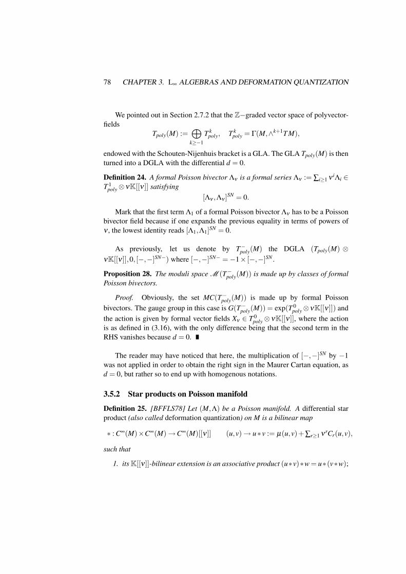
78 CHAPTER 3. L∞ ALGEBRAS AND DEFORMATION QUANTIZATION
We pointed out in Section 2.7.2 that the Z−graded vector space of polyvector-fields
Tpoly(M) :=⊕
k≥−1
T kpoly, T k
poly = Γ(M,∧k+1T M),
endowed with the Schouten-Nijenhuis bracket is a GLA. The GLA Tpoly(M) is thenturned into a DGLA with the differential d = 0.
Definition 24. A formal Poisson bivector Λν is a formal series Λν := ∑i≥1 ν iΛi ∈T 1
poly⊗νK[[ν ]] satisfying[Λν ,Λν ]SN = 0.
Mark that the first term Λ1 of a formal Poisson bivector Λν has to be a Poissonbivector field because if one expands the previous equality in terms of powers ofν , the lowest identity reads [Λ1,Λ1]SN = 0.
As previously, let us denote by T−poly(M) the DGLA (Tpoly(M) ⊗νK[[ν]],0, [−,−]SN−) where [−,−]SN− =−1× [−,−]SN .
Proposition 28. The moduli space M (T−poly(M)) is made up by classes of formalPoisson bivectors.
Proof. Obviously, the set MC(T−poly(M)) is made up by formal Poissonbivectors. The gauge group in this case is G(T−poly(M)) = exp(T 0
poly⊗νK[[ν]]) andthe action is given by formal vector fields Xν ∈ T 0
poly⊗ νK[[ν]], where the actionis as defined in (3.16), with the only difference being that the second term in theRHS vanishes because d = 0.
The reader may have noticed that here, the multiplication of [−,−]SN by −1was not applied in order to obtain the right sign in the Maurer Cartan equation, asd = 0, but rather so to end up with homogenous notations.
3.5.2 Star products on Poisson manifold
Definition 25. [BFFLS78] Let (M,Λ) be a Poisson manifold. A differential starproduct (also called deformation quantization) on M is a bilinear map
∗ : C∞(M)×C∞(M)→C∞(M)[[ν ]] (u,v)→ u∗ v := µ(u,v)+∑r≥1 νrCr(u,v),
such that
1. itsK[[ν ]]-bilinear extension is an associative product (u∗v)∗w = u∗(v∗w);
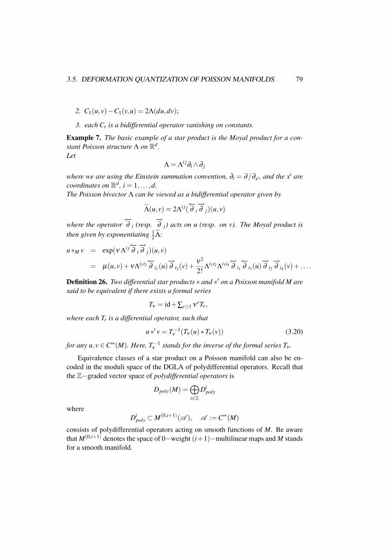
3.5. DEFORMATION QUANTIZATION OF POISSON MANIFOLDS 79
2. C1(u,v)−C1(v,u) = 2Λ(du,dv);
3. each Cr is a bidifferential operator vanishing on constants.
Example 7. The basic example of a star product is the Moyal product for a con-stant Poisson structure Λ on Rd .Let
Λ = Λi j∂i∧∂ j
where we are using the Einstein summation convention, ∂i = ∂/∂xi , and the xi arecoordinates on Rd , i = 1, . . . ,d.The Poisson bivector Λ can be viewed as a bidifferential operator given by
Λ(u,v) = 2Λi j(←−∂ i−→∂ j)(u,v)
where the operator←−∂ i (resp.
−→∂ j) acts on u (resp. on v). The Moyal product is
then given by exponentiating 12 Λ:
u∗M v = exp(ν Λi j←−∂ i−→∂ j)(u,v)
= µ(u,v)+νΛi1i2←−∂ i1(u)
−→∂ i2(v)+
ν2
2!Λi1i2Λi3i4
←−∂ i1←−∂ i3(u)
−→∂ i2−→∂ i4(v)+ . . . .
Definition 26. Two differential star products ∗ and ∗′ on a Poisson manifold M aresaid to be equivalent if there exists a formal series
Tν = id+∑r≥1 νrTr,
where each Tr is a differential operator, such that
u∗′ v = T−1ν (Tν(u)∗Tν(v)) (3.20)
for any u,v ∈C∞(M). Here, T−1ν stands for the inverse of the formal series Tν .
Equivalence classes of a star product on a Poisson manifold can also be en-coded in the moduli space of the DGLA of polydifferential operators. Recall thatthe Z−graded vector space of polydifferential operators is
Dpoly(M) =⊕
i∈ZDi
poly
whereDi
poly ⊂M(0,i+1)(A ), A := C∞(M)
consists of polydifferential operators acting on smooth functions of M. Be awarethat M(0,i+1) denotes the space of 0−weight (i+1)−multilinear maps and M standsfor a smooth manifold.
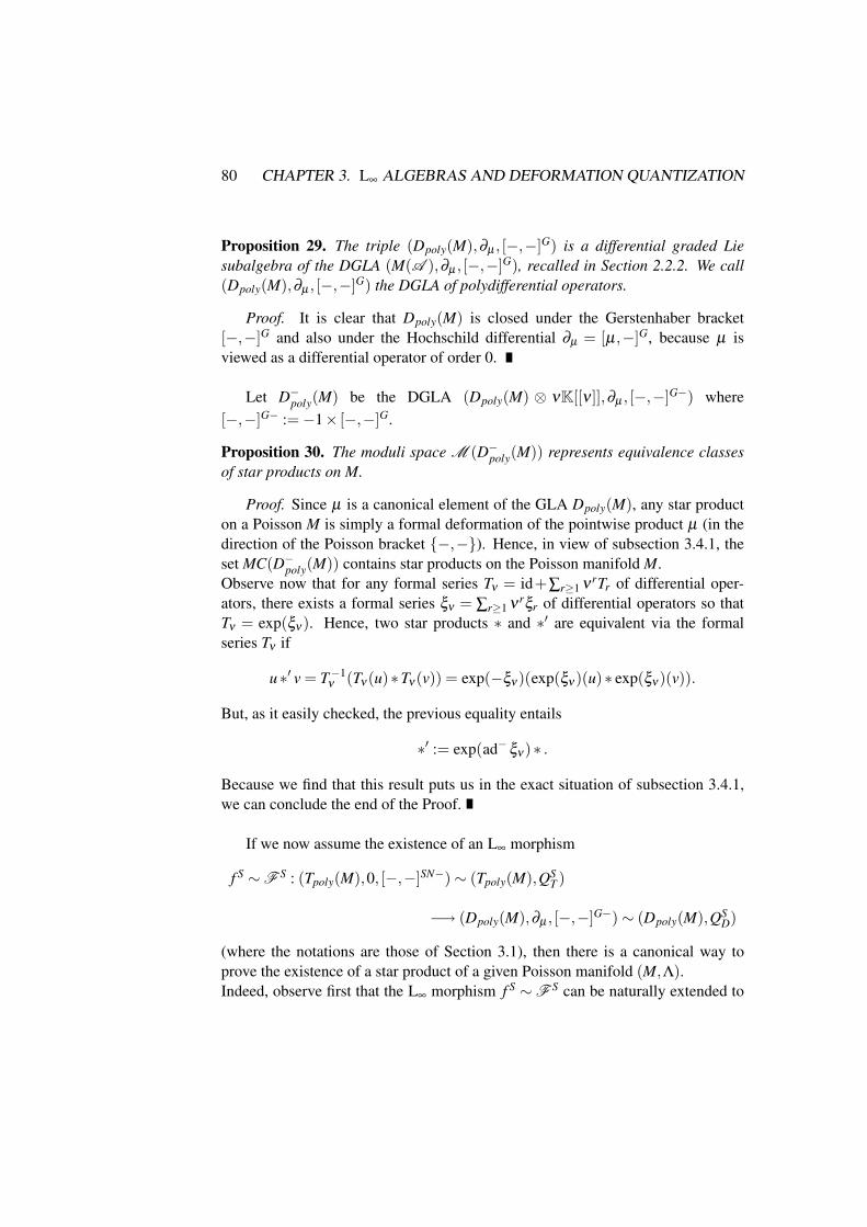
80 CHAPTER 3. L∞ ALGEBRAS AND DEFORMATION QUANTIZATION
Proposition 29. The triple (Dpoly(M),∂µ , [−,−]G) is a differential graded Liesubalgebra of the DGLA (M(A ),∂µ , [−,−]G), recalled in Section 2.2.2. We call(Dpoly(M),∂µ , [−,−]G) the DGLA of polydifferential operators.
Proof. It is clear that Dpoly(M) is closed under the Gerstenhaber bracket[−,−]G and also under the Hochschild differential ∂µ = [µ,−]G, because µ isviewed as a differential operator of order 0.
Let D−poly(M) be the DGLA (Dpoly(M) ⊗ νK[[ν ]],∂µ , [−,−]G−) where
[−,−]G− :=−1× [−,−]G.
Proposition 30. The moduli space M (D−poly(M)) represents equivalence classes
of star products on M.
Proof. Since µ is a canonical element of the GLA Dpoly(M), any star producton a Poisson M is simply a formal deformation of the pointwise product µ (in thedirection of the Poisson bracket −,−). Hence, in view of subsection 3.4.1, theset MC(D−
poly(M)) contains star products on the Poisson manifold M.Observe now that for any formal series Tν = id+∑r≥1 νrTr of differential oper-ators, there exists a formal series ξν = ∑r≥1 νrξr of differential operators so thatTν = exp(ξν). Hence, two star products ∗ and ∗′ are equivalent via the formalseries Tν if
u∗′ v = T−1ν (Tν(u)∗Tν(v)) = exp(−ξν)(exp(ξν)(u)∗ exp(ξν)(v)).
But, as it easily checked, the previous equality entails
∗′ := exp(ad− ξν)∗ .
Because we find that this result puts us in the exact situation of subsection 3.4.1,we can conclude the end of the Proof.
If we now assume the existence of an L∞ morphism
f S ∼F S : (Tpoly(M),0, [−,−]SN−)∼ (Tpoly(M),QST )
−→ (Dpoly(M),∂µ , [−,−]G−)∼ (Dpoly(M),QSD)
(where the notations are those of Section 3.1), then there is a canonical way toprove the existence of a star product of a given Poisson manifold (M,Λ).Indeed, observe first that the L∞ morphism f S ∼F S can be naturally extended to

3.5. DEFORMATION QUANTIZATION OF POISSON MANIFOLDS 81
the formal DGLA T−poly(M)∼ (Tpoly(M)⊗νK[[ν ]],QST ) by ν− linearity. Moreover,
as νΛ ∈MC(T−poly(M)), it follows from Proposition 22 that the element
F S∗ (ν ↓ Λ) = ∑∞s=1 ↑ νs
s! FSs (↓ Λ, . . . ,↓ Λ)
is a Maurer Cartan element of the set MC(D−poly(M)); remember that this set en-
codes the existence of star products. Thus, we obtain a star product ∗ on the Poissonmanifold (M,Λ), given by
∗ := ∑∞s=0
νs
s! (−1)s(s−1)
2 f Ss (Λ, . . . ,Λ)
where f0 is the pointwise product µ; remember that F Ss = (−1)
s(s−1)2 ↑ f S
s ↓∨s.Moreover, if f S ∼ F S is an L∞ quasi-isomorphism, it follows from Proposition28, Proposition 30 and Theorem 13, that there is a one-to-one correspondencebetween formal Poisson structures and star products.
Therefore, after having constructed an L∞ quasi-isomorphism from the DGLA(Tpoly(M),0, [−,−]SN−) to the DGLA (Dpoly(M),∂µ , [−,−]G−), the problem of ex-istence and classification of star products on a Poisson manifold M is solved. Suchan L∞ quasi-isomorphism was constructed by Kontsevich [Kon03] through the socalled formality Theorem.
Theorem 14. There exists an L∞ quasi-isomorphism from the DGLA(Tpoly(M),0, [−,−]SN−) to the DGLA (Dpoly(M),∂µ , [−,−]G−).
Kontsevich proved this Theorem in two steps. First, he gave an explicit for-mula for an L∞ quasi-isomorphism from the DGLA (Tpoly(M),0, [−,−]SN−) to theDGLA (Dpoly(M),∂µ , [−,−]G−) assuming that M = Rd . He then globalized thisformula on a general manifold using abstract arguments. The upcoming subsectionwill be concerned with outlining the first of Kontsevich’s steps as well as lookingat his explicit formula of a star product on Rd . The second step will be elaboratedin Chapter 4 through the angle of a more direct construction provided in [Dol05].
3.5.3 On the formality Theorem on Rd
Kontsevich’s star product on Rd
Kontsevich’s first main idea for constructing a star product on Rd was to provide agraphical representation for bidifferential operators. For the better comprehensionof this procedure we go back to the basic example of the Moyal product introduced
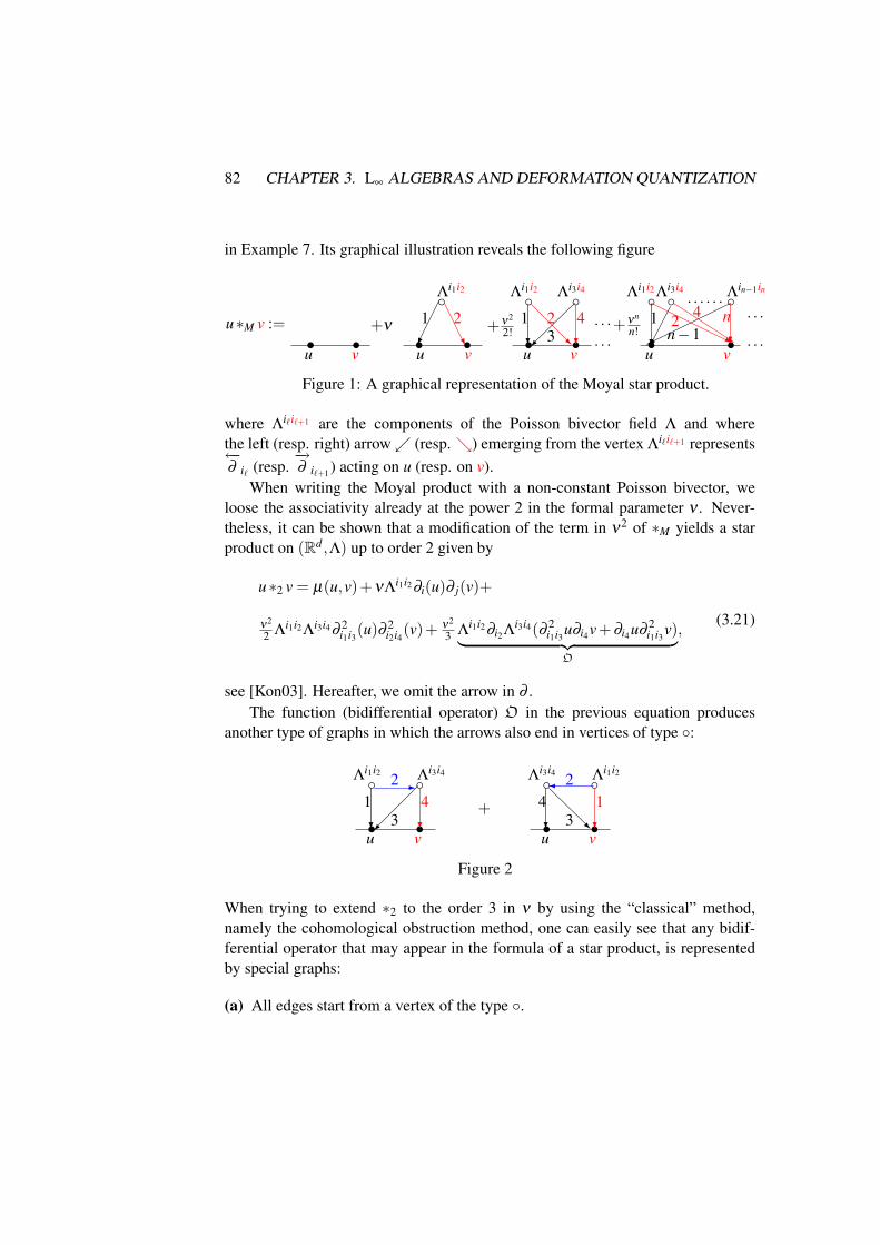
82 CHAPTER 3. L∞ ALGEBRAS AND DEFORMATION QUANTIZATION
in Example 7. Its graphical illustration reveals the following figure
u∗M v :=• •u v
+ν••
Λi1i2
1 2
u v® U
+ν2
2! • •u v
Λi1i2Λi3i4
?1
R2
ª3 ?4
. . .
. . .+νn
n!• •u v
Λi1i2
?
1s
2Λi3i4
® s
4. . . . . . Λ
in−1in
¼ ?n
n−1. . .
. . .
Figure 1: A graphical representation of the Moyal star product.
where Λi`i`+1 are the components of the Poisson bivector field Λ and wherethe left (resp. right) arrow (resp. ) emerging from the vertex Λi`i`+1 represents←−∂ i` (resp.
−→∂ i`+1) acting on u (resp. on v).
When writing the Moyal product with a non-constant Poisson bivector, weloose the associativity already at the power 2 in the formal parameter ν . Never-theless, it can be shown that a modification of the term in ν2 of ∗M yields a starproduct on (Rd ,Λ) up to order 2 given by
u∗2 v = µ(u,v)+νΛi1i2∂i(u)∂ j(v)+
ν2
2 Λi1i2Λi3i4∂ 2i1i3(u)∂ 2
i2i4(v)+ ν2
3 Λi1i2∂i2Λi3i4(∂ 2i1i3u∂i4v+∂i4u∂ 2
i1i3v)︸ ︷︷ ︸O
,(3.21)
see [Kon03]. Hereafter, we omit the arrow in ∂ .The function (bidifferential operator) O in the previous equation produces
another type of graphs in which the arrows also end in vertices of type :
• •u v
Λi1i2Λ
i3i4
1-2
ª3 ?
4?
+• •u v
Λi3i4Λ
i1i2
4R
2¾
3 ?
1?
Figure 2
When trying to extend ∗2 to the order 3 in ν by using the “classical” method,namely the cohomological obstruction method, one can easily see that any bidif-ferential operator that may appear in the formula of a star product, is representedby special graphs:
(a) All edges start from a vertex of the type .

3.5. DEFORMATION QUANTIZATION OF POISSON MANIFOLDS 83
(b) There are no loops, i.e. edges start and end at the same vertex
(c) There are 8 vertices and 6 edges; (mark that the p−th term (graph) of the Moyalproduct contain p+2 vertices and 2p edges).
However, particular care has to be devoted to the numerical coefficients assignedto these graphs so that the associativity holds up to order 3. One has to take intoaccount the Jacobi identity and symmetries; e.g. the Jacobi identity creates thefactor 1
3 in (3.21). Computations of these numerical coefficients are already quitelong and delicate for the order 3; these coefficients can be found in Theorem 1 ofChapter 4, where we explicitly constructed a star product up to order 3 on a generalPoisson manifold.In view of the above discussion, a natural question arises:Can we introduce an appropriate set of (suitable) graphs, and is there a naturalway of assigning numerical coefficients or weights to graphs so that a weightedsum for all (suitable) graphs will yield a star product? The following Theorem byKontsevich [Kon03] shows that the answer is yes.
Theorem 15. Let Λ be a Poisson bivector field on Rd . The formula
u∗K v = µ(u,v)+∞
∑p=1
ν p ∑Γ∈Gp,2
WΓ fΓ(Λ, . . . ,Λ︸ ︷︷ ︸p
)(u,v)
defines a star product on (Rd,Λ) for any u,v ∈C∞(Rd).
In this formula, Gp,2 denotes a subset of the set of graphs, the so calledadmissible graph, with n + 2 vertices and 2n edges. The bidifferential operatorsfΓ(Λ, . . . ,Λ) are constructed from the graph Γ, and WΓ are numerical coefficientsobtained as integrals over certain configuration spaces of a differential formdepending on Γ.
Our focus turns to introducing the set of graphs Gp,2 to a more general setting,namely to the context of the formality Theorem. We shall also look closely at theoperators fΓ since we will require their descriptions in Chapter 4. For a detailedexplanation of the configuration spaces and the coefficients WΓ, we refer the readerto [AMM02]. The proof of the Theorem 15 was given in [Kon03], [AMM02] andmany references therein.
Admissible graphs
Definition 27. An oriented graph Γ is a pair (V (Γ),E(Γ)) of two finite sets suchthat E(Γ) is a subset of V (Γ)×V (Γ).

84 CHAPTER 3. L∞ ALGEBRAS AND DEFORMATION QUANTIZATION
Elements of V (Γ) are the vertices of Γ, and elements of E(Γ) are its edges.For e = (v1,v2) ∈ E(Γ) we say that e starts at v1 and ends at v2. The set of edgesstarting (resp. ending) at a given vertex v will be denoted by Star(v) (resp. End(v)).
Definition 28. The set Gp,q, p,q ≥ 0 of admissible graphs consists of orientedgraphs satisfying the following proprieties:
• The set of vertices V (Γ) is decomposed into two ordered subsets V1(Γ) =a1,a2, . . . ,ap and V2(Γ) = b1,b2, . . . ,bq whose elements are called re-spectively vertices of the first type (aerial vertices) and vertices of the secondtype (ground vertices).
• The number of vertices of the two types verifies 2p+q−2≥ 0.
• All edges in E(Γ) start from a vertex of the first type.
• The edges emanating from a vertex a` can land on any vertex other than a`
itself, i.e. for every a` ∈V1(Γ) the pair (a`,a`) /∈ E(Γ) (no loops).
• The set of edges EΓ is endowed with a total order compatible with the orderof vertices
a1 < a2 < .. . < ap, b1 < b2 < .. . < bq,
namely if (](Star(a`)) = t`) for any 1 ≤ ` ≤ p, then the starting edges at a`
are labeled by numbers
t1 + t2 + . . .+ t`−1 +1, . . . , t1 + t2 + . . .+ t`.
Example 8. The first and the second graphs of Fig. 3 are admissible, while theothers are not.
•b1
•b2
•b3
a1
a2a3
?
2
*1
®
j
45
U
3
À ?6 7
Figure 3: Some examples of admissible and non-admissible graphs.
(i) (ii) (iii) (iv)
• •b1 b2
a1 a2
?
2 4
1
3
? • •b1 b2
a1 a2
6-
?= • •b1 b2
a1 a2-
?=
Definition 29. We denote by Gp,q the subclass of the set of admissible graphs with2p+q−2 edges, where p≥ 1 and q≥ 0 (and automatically 2p+q−2≥ 0).

3.5. DEFORMATION QUANTIZATION OF POISSON MANIFOLDS 85
Polydifferential operators associated to admissible graphs
Let Γ ∈ Gp,q be an admissible graph. Consider a collection of polydifferentialoperators Λ1, . . . ,Λp on Rd such that Λ` ∈ T k`
poly and k` = ](Star(a`))− 1 for any1≤ `≤ p, where a` ∈V1(Γ). For such data, we associate a polydifferential operatorfΓ(Λ1, . . . ,Λp) ∈ Dq−1
poly acting on q smooth functions u1, . . . ,uq on Rd as follows:
1. We associate to each vertex a` ∈ V1(Γ) the skew-symmetric tensor Λi1...ik`+1`
corresponding to the tensor Λ` via the natural identification.
2. We place a function u` at each vertex of the second type.
3. We label the edges of Star(Λ`) for any 1≤ `≤ p by the numbers k1 + . . .+k`−1 + `, . . . ,k1 + . . .+ k` + `, in other words, we identify E(Γ) with
1, . . . ,k1+1,k1+2, . . . ,k1+k2+2, . . . ,k1+. . .+kp−1+ p, . . . ,k1+. . .+kp+ p
4. We associate to any vertex c` of the first type (i.e. Λ`) or of the second type(i.e. u`), the operator
∂End(c`) =∂ s
∂it1. . .∂its
when End(c`) is made up by the edges ts ∈ E(Γ), for any 1≤ s≤ 2p+q−2.
5. Finally, we define the function fΓ(Λ1, . . . ,Λp)(u1, . . . ,uq) by
fΓ(Λ1, . . . ,Λp)(u1, . . . ,uq)
= ∑1≤i1,...,ik≤d
1≤k≤d
p
∏=1
∂End(Λ`)Λik1+...+k`−1+`,...,k1+...+k`+`
`
q
∏s=1
∂End(u j)u j.
As an example, the polydifferential operator corresponding to the first graph(resp. to the second graph) of Fig. 3 is given by
Λi1i2∂i1(Λi3i4i5)∂i3(Λ
i6i7)∂ 2i2i4(u1)∂i6(u2)∂ 2
i5i7(u3)
(resp.∂i3(Λ
i1i2)∂i1(Λi3i4)∂i2(u1)∂i4(u2).)
Thus, given any admissible graph Γ ∈ Gp,q, the above procedure provides amultilinear map
fΓ : Tpoly(M)× . . .×Tpoly(M)︸ ︷︷ ︸p
→ Dq−1poly

86 CHAPTER 3. L∞ ALGEBRAS AND DEFORMATION QUANTIZATION
that associates any collection of polyvectorfields Λ1, . . . ,Λp, Λ` ∈ T k`poly with a poly-
differential operator fΓ(Λ1, . . . ,Λp) ∈ Dq−1poly, which is given by the above detailed
procedure if k` = ](Star(a`))− 1 for any 1 ≤ ` ≤ p or equal to zero otherwise.Moreover, it is easily seen that fΓ is a (1− p) weight Z−graded skew-symmetricmap. Indeed, by definition we have
∑p`=1 k` = ∑p
`=1(](Star(a`))−1) = 2p+q−2− p = p+q−2;
so fΓ is a (1 − p) weight multilinear map because of the constructionfΓ(Λ1, . . . ,Λp) ∈ Dq−1
poly. The map fΓ is a Z−graded skew-symmetric mapbecause when permuting the order in which we label the edges, we get a signequal to the signature of the permutation; the polyvectorfields are of courseskew-symmetric and the partial derivatives are “symmetric”.
We are now prepared to state the Kontsevich formula for an L∞ quasi-isomorphism on Rd .
Kontsevich’s L∞ quasi-isomorphism on Rd
Theorem 16. For any p≥ 1, the (1− p) weight Z−graded skew-symmetric maps
f Kp = ∑
q≥0∑
Γ∈Gp,q
WΓ fΓ (3.22)
define an L∞ quasi-isomorphism
f K = ( f K1 , f K
2 , . . .) : (Tpoly(Rd),0, [−,−]SN−)→ (Dpoly(Rd),∂µ , [−,−]G−).
The proof of this theorem is based on the special choice of the numerical co-efficients WΓ, which are obtained as integrals over certain configuration spaces ofa differential form depending on Γ. We will not describe these coefficients WΓ andprove this Theorem. We refer again to [Kon03],[AMM02]. Let us just investigatethe first structure map f K
1 .By equation (3.22),
f K1 = ∑
q≥0∑
Γ∈G1,q
WΓ fΓ.
Now, the set G1,q contains only the graph Γq with one vertex of the first type,with 2×1 + q−2 = q edges and q ground vertices. Thus, for any polyvectorfieldΛ ∈ T q−1
poly , we associate the polydifferential operator given by
WΓqfΓq(Λ)(u1, . . . ,uq) = WΓqΛi1...iq∂i1(u1) . . .∂iq(uq).

3.5. DEFORMATION QUANTIZATION OF POISSON MANIFOLDS 87
Observe then that f K1 is a 0 weight linear map from Tpoly to Dpoly since each fΓ is
too for any Γ ∈ G1,q. It remains to prove that f K1 induces an isomorphism between
the corresponding cohomology, i.e.
f K1] : Tpoly = H(Tpoly(Rd),0)→ H(Dpoly(Rd),∂µ)
is an isomorphism. This is due to a previous result by Hochschild, Kostant andRosenberg [HKR62] which establishes an isomorphism between Tpoly(Rd) andH(Dpoly(Rd),∂µ).For any q≥ 0 this isomorphism is given by the map
hq(X1∧ . . .∧Xq)(u1, . . . ,uq) = 1q! ∑σ∈Sq(−1)σ X1(uσ(1)) . . .Xq(uσ(q))
where X` ∈ T 0poly, u` ∈C∞(Rd) and where Sq stands for the group of permutation
and (−1)σ denotes the signature of the permutation σ . Since it can be shown thatWΓq = 1
q! , we conclude that WΓqfΓq = hq.
Let us mention that this result was first proven for smooth affine algebraicvarieties in [HKR62]. A smooth version of it was outlined in [Vey75] and adetailed proof was given in [GR99]. Independently, Kontsevich gave also anotherproof for smooth manifold in [Kon03].
Remark 11. Note that the “formality” in the name of the Theorem stems fromhomotopy theory where a DGLA is called formal if it is quasi-isomorphic to itscohomology, regarded as a DGLA with zero differential and the induced bracket. Inother words, the formality Theorem states that Dpoly(M) is formal for any smoothmanifold M.
In Chapter 4, we shall analyze Dolgushev’s globalization procedure [Dol05]for the Kontsevich formality quasi-isomorphism f K . This construction needs cer-tain particular proprieties of the Kontsevich quasi-isomorphism f K , which are pre-sented in the following Theorem.
Theorem 17. Kontsevich’s quasi-isomorphism
f K : (Tpoly(Rd),0, [−,−]SN−)→ (Dpoly(Rd),∂µ , [−,−]G−)
satisfies the following proprieties

88 CHAPTER 3. L∞ ALGEBRAS AND DEFORMATION QUANTIZATION
1. f K is also an L∞ quasi-isomorphism in the formal setting, i.e. one canreplace Rd by the space R[[x1, . . . ,xd ]] of formal power series in x =(x1, . . . ,xd) ∈ Rd with real coefficients, because the coefficients of the poly-differential operators f K
` are polynomial functions of the derivatives of thecoordinates of the polyvectorfields.
2. f K is equivariant with respect to linear transformations of the coordinatesx1, . . . ,xd .
3. If p≥ 2, thenf Kp (X1,X2, . . . ,Xp) = 0 (3.23)
for any set of vector fields X1,X2, . . . ,Xp ∈ T 0poly.
4. If n≥ 2 and X ∈ T 0poly is linear in the coordinates x1, . . . ,xd , then for any set
of polyvectorfields Λ2, . . . ,Λn
f Kp (X ,Λ2, . . . ,Λp) = 0. (3.24)
Points (3) and (4) result from an explicit calculation of certain integrals overconfiguration spaces, see [Kon03].As a concluding act, let us observe that the coefficients of the polydifferential op-erators f K
p (Λ1, . . . ,Λp) for any p ≥ 1 are given by universal (admissible) poly-nomials in the polyvectorfields Λ1, . . . ,Λp and their partial derivatives, where theconcatenations are given by the subset Gp,q, q ≥ 0, of the admissible graph Gp,q;the concatenations only arise between different polyvectorfields because there areno loops, see Example 8.
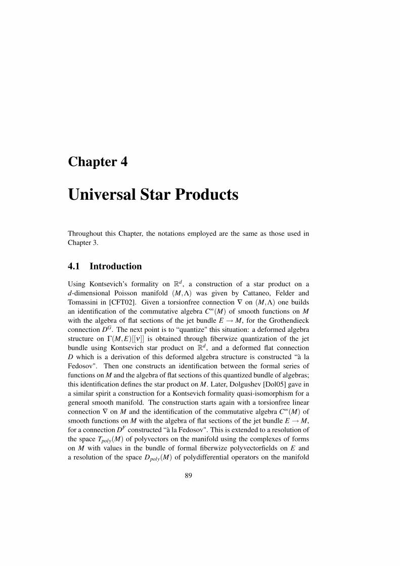
Chapter 4
Universal Star Products
Throughout this Chapter, the notations employed are the same as those used inChapter 3.
4.1 Introduction
Using Kontsevich’s formality on Rd , a construction of a star product on ad-dimensional Poisson manifold (M,Λ) was given by Cattaneo, Felder andTomassini in [CFT02]. Given a torsionfree connection ∇ on (M,Λ) one buildsan identification of the commutative algebra C∞(M) of smooth functions on Mwith the algebra of flat sections of the jet bundle E → M, for the Grothendieckconnection DG. The next point is to “quantize" this situation: a deformed algebrastructure on Γ(M,E)[[ν ]] is obtained through fiberwize quantization of the jetbundle using Kontsevich star product on Rd , and a deformed flat connectionD which is a derivation of this deformed algebra structure is constructed “à laFedosov". Then one constructs an identification between the formal series offunctions on M and the algebra of flat sections of this quantized bundle of algebras;this identification defines the star product on M. Later, Dolgushev [Dol05] gave ina similar spirit a construction for a Kontsevich formality quasi-isomorphism for ageneral smooth manifold. The construction starts again with a torsionfree linearconnection ∇ on M and the identification of the commutative algebra C∞(M) ofsmooth functions on M with the algebra of flat sections of the jet bundle E → M,for a connection DF constructed “à la Fedosov". This is extended to a resolution ofthe space Tpoly(M) of polyvectors on the manifold using the complexes of formson M with values in the bundle of formal fiberwize polyvectorfields on E anda resolution of the space Dpoly(M) of polydifferential operators on the manifold
89

90 CHAPTER 4. UNIVERSAL STAR PRODUCTS
using the complexes of forms on M with values in the bundle of formal fiberwizepolydifferential operators on E. The fiberwize Kontsevich L∞ quasi-morphismis then twisted and contracted to yield an L∞ quasi-morphism from Tpoly(M) toDpoly(M).
In the following, we introduce the notion of universal formality L∞ quasi-isomorphism and the notion of universal deformation quantization.Given a torsionfree linear connection ∇ on a manifold M, any polydifferential op-erator Op : C∞(M)×k →C∞(M) writes in a unique way as
Op(u1, . . . ,uk) = ∑I1,...,Ik
OpI1,...,Ik ∇symI1
u1 . . .∇symIk
uk (4.1)
where the I1, . . . , Ik are multiindices and ∇symI u is the symmetrized covariant deriva-
tive of order |I| of u:
∇symI u = ∑
σ∈Sm
1m!
∇miσ(1)...iσ(m)
u for I = (i1, . . . , im),
where ∇mi1...imu := ∇mu(∂i1 , . . . ,∂im) with ∇mu defined inductively by ∇u := d u and
∇mu(X1, . . . ,Xm) = (∇X1(∇m−1u))(X2, . . . ,Xm).The tensors OpI1,...,Ik are covariant tensors of order |I1|+ . . .+ |Ik| which are sym-metric within each block of Ir indices; they are called the tensors associated to Opfor the given connection.
Definition 30. For any integer k ≥ 1, a universal k−polyvectorfields-related poly-differential operator will be the association to any manifold M, any torsionfreeconnection ∇ on M and any collection of polyvectorfields Λ1, . . . ,Λk ∈ Tpoly(M),of a polydifferential operator Op(M,∇,Λ1,...,Λk) : C∞(M)× j → C∞(M), so that, thetensors associated to Op(M,∇,Λ1,...,Λk) for ∇ are given by universal polynomials inΛ1, . . . ,Λk, the curvature tensor R and their covariant multiderivatives, involvingconcatenations and the association being linear in each Λi.We shall say that a universal k−polyvectorfields-related polydifferential operatoris of no-loop type if the concatenations only arise between different terms, notwithin a given term (i.e.
(∇rΛ`)··i··s··(∇sΛ`′)·· j··r··∇sym··i·· j··
is of no-loop type but
(∇··t··Λ`)··t··i··∇sym··i·· or Rr
strΛ··s··i··` Λ··t·· j··`′ ∇sym
··i·· j··
are not).

4.2. AN EXAMPLE AT ORDER 3 91
Definition 31. A universal Poisson-related polydifferential operator will be the as-sociation to any manifold M, any torsionfree connection ∇ on M, any Poissontensor Λ on M and any integer k ≥ 1, of a universal k−polyvectorfields-relatedpolydifferential operator Op(M,∇,Λ,...,Λ), which will be denoted by Op(M,∇,Λ).We shall say that a universal Poisson-related polydifferential operator is of no-looptype if Op(M,∇,Λ) is too.We shall say that the universal Poisson-related polydifferential operator Op(X ,∇,Λ)
is a polynomial of degree r in the Poisson structure if r = k.
Definition 32. A universal formality L∞ quasi-isomorphism will be the associationto any given manifold M and any torsionfree linear connection ∇ on M, of anL∞ quasi-morphism f = ( f1, f2, . . .) from the DGLA (Tpoly(M),0, [−,−]SN−) to theDGLA (Dpoly(M),∂µ , [−,−]G−), where, for any k ≥ 1, each structure map fk is ak−polyvectorfields-related polydifferential operator of no-loop type.
Definition 33. A universal star product ∗ = µ + ∑r≥1 νrCr will be the associationto any manifold M, any torsionfree connection ∇ on M and any Poisson tensor Λon M, of a differential star product ∗(M,∇,Λ) := µ +∑r≥1 νrC(M,∇,Λ)
r where each Cr
is a universal Poisson-related bidifferential operator of no-loop type, which is apolynomial of degree r in the Poisson structure.
An example of a universal star product at order 3 is given in section 4.2.Unicity at order 3 is studied in section 4.3 using universal Poisson cohomology.This, we compute for universal Poisson-related bidifferential operators of order 1in each argument defined by low order polynomials in the Poisson structure.The existence of a universal formality L∞ quasi-isomorphism and a universal starproduct are implied by the Dolgushev’s globalization procedure [Dol05]. The glob-alization proof of Cattaneo, Felder and Tomassini [CFT02, CF01], using the expo-nential map of a torsionfree linear connection, gives also the existence of a univer-sal star product. We show these existences in sections 4.5 and 4.6, stressing firstthe relations between the resolutions involved in the two constructions in section4.4.
4.2 An example at order 3
Theorem 1. There exists a universal star product up to order three, which asso-ciates to a Poisson manifold (M,Λ) and a torsionfree linear connection ∇ on M,

92 CHAPTER 4. UNIVERSAL STAR PRODUCTS
the star product at order three defined by
u∗(M,∇,Λ)3 v = µ(u,v)+νu,v+ν2C(M,∇,Λ)
2 (u,v)+ν3C(M,∇,Λ)3 (u,v), u,v∈C∞(M)
(4.2)C(M,∇,Λ)
2 (u,v)
= 12 ΛkrΛls∇2
klu∇2rsv+ 1
3 Λkr∇rΛls(∇2klu∇sv+∇su∇2
klv)+ 16 ∇lΛkr∇kΛls∇ru∇sv,
(4.3)and
C(M,∇,Λ)3 (u,v)=
16
S(M,Λ) 3∇ (u,v)=−1
6Λls(LXu∇) j
kl(LXv∇)kjs with Xu = i(du)Λ,
(4.4)where LXu∇ is the tensor defined by the Lie derivative of the connection ∇ in thedirection of the Hamiltonian vector field Xu
(LXu∇) jkl = Λi j∇3
kliu+∇kΛi j∇2liu+∇lΛi j∇2
kiu+∇2klΛ
i j∇iu+R jiklΛ
si∇su.
This can be seen by direct computation.
Remark 12. The operator S(M,Λ) 3∇ was introduced by Flato, Lichnerowicz and
Sternheimer [FLS76]; it is a Chevalley-cocycle on (M,Λ), i.e.
+©u,v,w
S(M,Λ) 3
∇ (u,v),w
+S(M,Λ) 3∇ (u,v ,w) = 0,
where +©u,v,w
denotes the sum over cyclic permutations of u,v,w.
For this universal star product at order 3, there exists a universal Poisson-related-differential-operator-valued 1-form D defined as follows:
Proposition 31. Given any Poisson manifold (M,Λ), any torsionfree linear con-nection ∇ on M, and any vector field X on M, the differential operator D(M,∇,Λ)
Xdefined by
D(M,∇,Λ)X v = Xv−ν2 1
6Λls(LX ∇) j
kl(LXv∇)kjs, v ∈C∞(M)
verifies at order 3 in ν
D(M,∇,Λ)X (u∗(M,∇,Λ)
3 v)− (D(M,∇,Λ)X u)∗(M,∇,Λ)
3 v−u∗(M,∇,Λ)3 (D(M,∇,Λ)
X v)
= ddt |t=0u∗(M,∇,φ X
t∗Λ)3 v+O(ν4).

4.3. UNIVERSAL POISSON COHOMOLOGY 93
where φ Xt denotes the flow of the vectorfield X.
If X is a Hamiltonian vector field corresponding to a function u ∈ C∞(M), thenD(M,∇,Λ)
Xucoincides with the inner derivation at order 3 of ∗3 defined by the function
u, i.e.
D(M,∇,Λ)Xu
v =1
2ν(u∗(M,∇,Λ)
3 v− v∗(M,∇,Λ)3 u).
4.3 Equivalence of universal star products – UniversalPoisson cohomology
Lemma 1. • Any universal star product ∗ = µ + ∑r≥1 νrCr is a natural starproduct, i.e. each bidifferential operator Cr is of order at most r in each ar-gument. Indeed Cr is a universal r−Poisson-related bidifferential operator;this implies, in view of the Bianchi’s identities for the curvature tensor, thatCr is of order at most r in each argument.
• The universal Poisson-related bidifferential operator C1 of any universal starproduct is necessarily the Poisson bracket C(M,∇,Λ)
1 = Λi j∇i∧∇ j.
• The Gerstenhaber bracket [−,−]G of two universal Poisson-related polyd-ifferential operator of degree k and l in Λ, is a universal Poisson-relatedpolydifferential operator of degree k + l in Λ.
• If a universal Poisson-related p-differential operator C is a Hochschild p-cocycle ( where ∂µ = [µ,−]G denotes the Hochschild differential) then C =A + ∂µB where A a universal Poisson-related p-differential operator whichis of order 1 in each argument and is the totally skew-symmetric part of C,and where B is a universal Poisson-related (p−1)-differential operator.
The last point comes from the explicit formulas [GR99] for the tensors associ-ated to B in terms of those associated to C when one is given a connection.
Definition 34. A universal Poisson p-cocycle is a universal Poisson-relatedp-differential skew-symmetric operator C of order 1 in each argument whichis a cocycle for the Chevalley cohomology for the adjoint representation of(C∞(M),−,−), i.e. with the coboundary defined by
δΛC(u1, . . . ,um+1) =m+1
∑i=1
(−1)iui,C(u1, . . . ui . . . ,um+1)
+∑i< j
(−1)i+ jC(ui,u j,u1 . . . ui . . . u j . . . ,um+1).

94 CHAPTER 4. UNIVERSAL STAR PRODUCTS
which can be written as a multiple of
[Λ,C(M,∇,Λ)]NR
where skew indicates the skew-symmetrization in all its arguments of an operator.Equivalently, a universal Poisson p-cocycle C is defined by a universal Poissonrelated skew-symmetric p-tensor c (with C(u1, . . . ,up) = c(du1, . . . ,dup)) so that
[Λ,c(M,∇,Λ)]SN = 0
A universal Poisson p-cocycle C is a universal Poisson coboundary if thereexists a universal Poisson-related skew-symmetric (p− 1)-differential operator Cof order 1 in each argument so that
C(M,∇,Λ) = δΛB(M,∇,Λ)(= [Λ,B(M,∇,Λ)]NR);
(equivalently, if there exists a universal Poisson related tensor b so that c(M,∇,Λ) =[Λ,b(M,∇,Λ)]SN).The universal Poisson cohomology H p is the quotient of the space of universalPoisson p-cocycles by the space of universal Poisson p-coboundaries.We can restrict ourselves to the space of universal Poisson p-cocycles defined bypolynomials of degree k in the Poisson structures and make the quotient by thespace of universal Poisson coboundaries defined by polynomials of degree k− 1.We speak then of the universal Poisson p-cohomology of degree k in the Poissonstructure and we denote it by H p
polk. We can further restrict ourselves to universalPoisson related tensors (or operators of order 1 in each argument) of no-loop type.
Definition 35. If ∗= µ +∑r≥1 νrCr is a universal star product and if E = ∑∞r=2 νEr
is a formal series of universal differential operators vanishing on constants, of no-loop type, with each Er a polynomial of degree r in the Poisson structure, then theseries ∗′ defined by
∗′ = (expadE)∗is an equivalent universal star product. We say that ∗ and ∗′ are universally equiv-alent.
Lemma 2. If ∗ and ∗′ are universal star products which coincide at order k in thedeformation parameter ν , then, by the associativity relation at order k, C′k−Ck isa universal Hochschild 2-cocycle of no-loop type which is a polynomial of degreek in the Poisson structure. Furthermore, associativity at order k+1 implies that itsskew-symmetric part p2 is a universal Poisson 2-cocycle :
+©u,v,w
pM,∇,Λ
2 (u,v),w
+ pM,∇,Λ2 (u,v ,w) = 0,

4.3. UNIVERSAL POISSON COHOMOLOGY 95
where +©u,v,w
denotes the sum over cyclic permutations of u,v,w.
If it is a universal Poisson 2-coboundary of no-loop type, then there is a aformal series E of universal differential operators vanishing on constants suchthat (expadE)∗ and ∗′ coincide at order k +1.
In particular, two universal star products are universally equivalent ifH2
(no−loop,pol) = 0. They are always equivalent at order k in the deformationparameter ν if H2
(no−loop)pol j = 0 ∀1≤ j ≤ k.
Consider now any universal star product ∗= µ +∑r≥1 νrCr. We automaticallyhave that C1 is the Poisson bracket. Associativity at order 2 yields ∂C2 = ∂C(M,∇,Λ)
2so
C2(u,v) = C(M,∇,Λ)2 (u,v)+ p2(u,v)+∂E2(u,v)
and the skew-symmetric part of associativity at order 3 yields that p2 is a universalPoisson 2-cocycle (which is a polynomial of degree 2 in the Poisson structure).
Proposition 32. The spaces H2pol2(Λ) and H2
(no−loop)pol2(Λ) of universal Poisson2-cohomology of degree 2 in the Poisson structure vanish.
Proof. The universal skew-symmetric 2-tensors of degree 2 in Λ are combina-tions of
∇sΛir∇rΛ js∇i∧∇ j,
(∇2rsΛ
irΛ js−∇2rsΛ
jrΛis)∇i∧∇ j,
(ΛirΛstR jrst −Λ jrΛstRi
rst)∇i∧∇ j,
ΛriΛs jRtrst∇i∧∇ j.
The only universal cocycles are the multiples of
ΛriΛs jRtrst∇i∧∇ j
and those are the boundaries of the multiples of ∇rΛir∂i. Remark that there are nococycles of no-loop type.
Thus, universal star product at order 2 are unique modulo equivalence and onecan assume that C2 = C(M,∇,Λ)
2 . Then the skew-symmetric part of the Hochschild2-cocycle C3−C(M,∇,Λ)
3 is a universal Poisson 2-cocycle of no-loop type which isa polynomial of degree 3 in the Poisson structure.

96 CHAPTER 4. UNIVERSAL STAR PRODUCTS
Proposition 33. The space H2(no−loop)pol3(Λ) of universal Poisson 2-cohomology
of no-loop type and of degree 3 in the Poisson structure vanishes.
Proof. We consider all possible universal Poisson 2-cochains of no loop typewhich are polynomials of degree 3 in the Poisson structure. They are defined byuniversal skew-symmetric 2-tensors of degree 3 in Λ which are combinations withconstant coefficients of the different concatenations (with no loops) of
Λ··Λ··Λ··(∇2··R)···· Λ··Λ··Λ··R····R
····,
Λ··(∇·Λ)··(∇·Λ)··R···· Λ··Λ··(∇·Λ)··(∇·R)····Λ··Λ··(∇2
··Λ)··R···· Λ··(∇2··Λ)··(∇2
··Λ)·· (∇2··Λ)··(∇·Λ)··(∇·Λ)··.
Using the symmetry properties of R, the Bianchi’s identities and the fact that Λ isa Poisson tensor, one is left with a combination with constant coefficients of 49independent terms.Universal 2-coboundaries come from the boundaries of universal 1-tensors of de-gree 2 in Λ; such 1-tensors are given by combinations with constant coefficients ofconcatenations of
Λ··Λ··(∇·R)···· Λ··(∇·Λ)··R····.
Hence, modulo universal coboundaries, one can assume that the coefficients of 4of the 49 terms in a universal cochain are zero.The cohomology that we are looking for is then given by the combinations withconstant coefficients of the remaining 45 terms which are cocycles (for all possiblechoices of manifold, Poisson structure Λ and connection ∇.)Let C be a combination of those 45 terms. The cocycle condition is [Λ,C]SN = 0.We plug in examples of Poisson structures and connections and impose this cocyclecondition. This shows that all 45 coefficients must vanish.It is enough, for instance, to consider the example on R4, with the non vanishingcoefficients of the connection defined by
Γ112 = x3
1, Γ114 = x4 Γ2
11 = x21, Γ2
13 = 1, Γ222 = 1, Γ2
14 = x3, Γ313 =−x4,
Γ333 = 1, Γ3
44 =−x2x3x4, Γ411 = 1, Γ4
13 = 1, Γ422 = x1, Γ3
44 =−3.
and the quadratic Poisson structure defined by
Λ = ∑1=i< j=4
xix j∂
∂xi∧ ∂
∂x j
From this example, one gets that 41 of the 45 coefficients have to vanish. One isleft with a combination with constant coefficients of four terms and an example

4.4. GROTHENDIECK- AND DOLGUSHEV-RESOLUTION 97
with constant Poisson structure in dimension 7 shows that all those coefficientsmust vanish. The non vanishing coefficients of this example are:
Λ12 = 1 Λ15 = 1 Λ17 = 1 Λ25 = 1 Λ26 = 2 Λ27 = 2
Λ34 = 1 Λ37 = 3 Λ46 = 1 Λ47 = 4 Λ56 = 1 Λ57 = 5 Λ67 = 6.
Γ112 = 1 Γ1
62 = x7 Γ177 =−1 Γ2
17 = x1 Γ313 = x6 Γ4
11 = 1Γ4
22 = 1 Γ433 = 2Γ4
77 = 3 Γ512 = x1x5 Γ5
33 = x2 Γ611 = 1
Γ644 = x2 Γ6
44 = x5 Γ711 = x7 Γ7
44 = x3 Γ717 = x1.
Corollary 3. Any universal star product is universally equivalent to one whoseexpression at order 3 is given by formula (4.2).
4.4 Grothendieck- and Dolgushev-resolution of the spaceof functions
Our purpose in this section is to prove that the Fedosov-resolution of the algebra ofsmooth functions constructed in Dolgushev [Dol05] coincides with its resolutiongiven by Cattaneo, Felder and Tomassini in [CFT02]. We also give explicitly theidentification of smooth functions, polyvectorfields and polydifferential operatorson M with flat sections in the corresponding bundles.
Let M be a d-dimensional manifold and consider the jet bundle E → M (thebundle of infinite jet of functions) with fibers R[[y1, . . . ,yd]] (i.e. formal powerseries in y ∈ Rd with real coefficients) and transition functions induced from thetransition functions of the tangent bundle T M. Thus
E = F(M)×Gl(d,R)R[[y1, . . . ,yd ]] (4.5)
where F(M) is the frame bundle. Remark that E can be seen as the formallycompleted symmetric algebra of the cotangent bundle T ∗M; a section s ∈ Γ(M,E)can be written in the form
s = s(x;y) =∞
∑p=0
si1...ip(x)yi1 · · ·yip
with repeated indices varying from 1 to d, and where the si1...ip are componentsof symmetric covariant tensors on M. This bundle E is denoted S M by Dolgushev.

98 CHAPTER 4. UNIVERSAL STAR PRODUCTS
The construction of a star product on a d-dimensional Poisson manifold (M,Λ)given by Cattaneo, Felder and Tomassini in [CFT02], using a linear torsionfreeconnection ∇ on the manifold M, starts with the identification of the commutativealgebra C∞(M) of smooth functions on M with the algebra Z 0(Γ(M,E),DG) offlat sections of the jet bundle E →M , for the Grothendieck connection DG (whichis constructed using ∇). Let us recall this construction.
The exponential map for the connection ∇ gives an identification
expx : U ∩TxM →M y 7→ expx(y) (4.6)
at each point x, of the intersection of the tangent space TxM with a neighborhoodU of the zero section of the tangent bundle T M with a neighborhood of x in M.
To a function u ∈ C∞(M), one associates the section uφ of the jet bundle E → Mgiven, for any x ∈M by the Taylor expansion at 0 ∈ TxM of the pullback u expx.
Lemma 3. The section uφ is given by:
uφ (x;y) = u(x)+ ∑n>0
1n!
∇ni1...inu(x)yi1 . . .yin = u(x)+ ∑
n>0
1n!
∇n,symi1...in u(x)yi1 . . .yin .
(4.7)
Proof. In local coordinates xi’s one has
ddt
u(expx ty) =d
∑k=1
(∂xk u)(expx ty)ddt
(expx ty)k
and
d2
dt2 u(expx ty)
= ∑k,l(∂ 2xkxl u)(expx ty) d
dt (expx ty)k ddt (expx ty)l +∑d
k=1(∂xk u)(expx ty) d2
dt2 (expx ty)k.
The definition of the exponential map imply that
d2
dt2 (expx ty)k =−∑r,s
Γkrs(expx ty)
ddt
(expx ty)r ddt
(expx ty)s (4.8)
henced2
dt2 u(expx ty) = ∑k,l
(∇2klu)(expx ty)
ddt
(expx ty)k ddt
(expx ty)l.

4.4. GROTHENDIECK- AND DOLGUSHEV-RESOLUTION 99
By induction, one gets
dn
dtn u(expx ty) = ∑k1,...,kn
(∇nk1...kn
u)(expx ty)ddt
(expx ty)k1 . . .ddt
(expx ty)kn
and the result follows at t = 0.
Definition 36. [CF01] The Grothendieck connection DG on E is defined by:
DGX s(x;y) :=
ddt |t=0
s(x(t); exp−1x(t)(expx(y))) (4.9)
for any curve t → x(t) ∈ M representing X ∈ TxM and for any s ∈ Γ(M,E). It islocally given by
DGX =
d
∑i=1
X i
∂xi +∑
k∑
j
(∂φx
∂y
−1)k
j
∂φ j
∂xi ∂yk
(4.10)
where φx(y) = φ(x,y) is the Taylor expansion of expx y at y = 0:
φ(x,y)k = xk + yk
−12 ∑rs Γk
rs(x)yr ys + 13! ∑rst
(−(∂xr Γkst)(x)+2∑u Γu
rs(x)Γkut(x)
)yr ys yt +O(y4).
Remark 13. • From the definition (4.9) it is clear that DG is flat (DGX DG
Y −DGY
DGX = DG
[X ,Y ]).• It is also obvious that DG(uφ ) = 0 ∀u ∈C∞(M).
Lemma 4. [CF01] Introducing the operator on E-valued forms on M
δ = ∑i
dxi ∂∂ yi , (4.11)
one can writeDG =−δ +∇′+A, (4.12)
where
∇′ = ∑i
dxi
(∂xi −∑
jkΓk
i j y j ∂yk
)(4.13)
is the covariant derivative on E associated to ∇ and where A is a 1-form on M withvalues in the fiberwize vectorfields on E,
A(x;y) =: ∑ik
dxi Aki (x;y)∂yk = ∑
ikdxi
(−1
3 ∑rs
Rkris(x)y
rys +0(y3))
∂yk . (4.14)

100 CHAPTER 4. UNIVERSAL STAR PRODUCTS
One extends as usual the operator DG to the space Ω(M,E) of E-valued formson M:
DG =−δ +∇′+A with ∇′ = d−∑i jk
dxiΓki j y j ∂yk . (4.15)
One introduces the operator δ ∗ = ∑ j y j i( ∂∂ x j ) on Ω(M,E). Clearly (δ ∗)2 = 0,δ 2 =
0 and for any ω ∈ Ωq(M,Ep), i.e. a q-form of degree p in y, we have (δδ ∗ +δ ∗δ )ω = (p+q)ω.Defining, for any ω ∈Ωq(M,Ep)
δ−1ω =1
p+qδ ∗ω when p+q 6= 0
= 0 when p = q = 0
we see that any δ -closed q-form ω of degree p in y, when p+q > 0, writes uniquelyas ω = δσ with δ ∗σ = 0; σ is given by σ = δ−1ω .One proceeds by induction on the degree in y to see that the cohomology of DG isconcentrated in degree 0 and that any flat section of E is determined by its part ofdegree 0 in y. Indeed a q-form ω is DG-closed if and only if δω = (∇′+A)ω; thisimplies that δωp = 0 for ωp the terms of lowest order (p) in y. When p + q > 0we can write ωp = δ (δ−1ωp) and ω −DG(δ−1ωp) has terms of lowest order atleast p+1 in y. Remark that given any section s of E then s(x;y = 0) determines asmooth function u on M. If DGs = 0, then s−uφ is still DG closed. By the above,its terms of lowest order in y must be of the form δσ hence must vanish since wehave a 0-form. Hence we have:
Lemma 5. [CF01] Any section of the jet bundle s∈Γ(E) is the Taylor expansion ofthe pullback of a smooth function u on M via the exponential map of the connection∇ if and only if it is horizontal for the Grothendieck-connection DG:
s = uφ for a u ∈C∞(M)⇔ s ∈ Γhor(E) := s′ ∈ Γ(E) |DGs′ = 0. (4.16)
Furthermore, the cohomology of DG is concentrated in degree 0. In other word,one obtains a “Grothendieck-resolution” of the algebra of smooth functions, i.e.
H•(Ω(M,E),DG) = H0(Ω(M,E),DG) = Γhor(E)∼= C∞(M).
Remark 14. When a q-form ω is DG exact, we have written ω = DGσ wherethe tensors defining σ are given by universal polynomials (with no-loop concate-nations) in the tensors defining ω , the tensors defining A, the curvature of theconnection, and their iterated covariant derivatives.

4.4. GROTHENDIECK- AND DOLGUSHEV-RESOLUTION 101
Lemma 6. The 1-form A on M with values in the fiberwize vectorfields on E isgiven by A(x;y) =: ∑ik dxi Ak
i (x;y)∂yk where the Aki are universal polynomials given
by (no-loop) concatenations of iterative covariant derivatives of the curvature; theyare of the form
∑(∇...R) j1i·· (∇...R) j2
j1·· . . .(∇...R)kjs−1·· y
· . . .y·. (4.17)
In particular δ−1A = 0 since the curvature is skew-symmetric in its first two lowerarguments. The 1-form A is uniquely characterized by the fact that δ−1A = 0 andthe fact that DG =−δ +∇′+A is flat, i.e;
(DG
)2 = 0 which is equivalent to
δA = R∇′ +∇′A+12[A,A] (4.18)
for
12[A,A](X ,Y ) := [A(X),A(Y )] and R∇′ =−1
2Rl
i jkdxi∧dx jyk ∂∂yl .
Proof. Any section s ∈ Γ(M,E) writes ∑∞p=0 sp
i1...ip(x)yi1 · · ·yip with symmetric
p-covariant tensors spi1...ip
. Write
A(x;y) = ∑r≥2
dxi(A(r)(x))ki, j1... jr y
j1 . . .y jr ∂yk
with (A(2)(x))ki,rs =−1
3 ∑rs Rkris(x)y
rys. Then the covariant tensors of DGX s are given
by the symmetrization of
(DG
X s)p
=−i(X)sp+1 +∇X sp +p−2
∑r=0
(A(p−r)(X))k ∂yk sr+1.
The fact that DG(uφ ) = 0 ∀u ∈C∞(M) implies the expression given in the lemmafor A. Indeed, the symmetric tensors defining uφ are given by 1
p! ∇p,symu and we
must have
0 =(
DG∂xi
uφ
)p
j1... jp=− 1
(p+1)!(∇p+1,symu)i j1... jp +
1p!
(∇(∇p,symu))i j1... jp
+p−2
∑r=0
(A(p−r)(x)
)k
i, j1... jp−r
1r!
(∇r+1,symu)k jp−r+1... jp
102 CHAPTER 4. UNIVERSAL STAR PRODUCTS
with the last terms symmetrized in the j′s. The commutation of covariant deriva-tives of a q-form ω gives
(∇p+2u)kl j1... jp − (∇p+2u)lk j1... jp =−p
∑r=0
Rskl jr(∇
pu) j1... jr−1s jr+1... jp
and implies by induction that (∇(∇p,symu))i j1... jp − (∇p+1,symu)i j1... jp is a univer-sal expression contracting covariant derivatives of the curvature tensor with lowercovariant derivatives of u of the form
(∇...R)t1i·· (∇...R)t2
t1·· . . .(∇...R)sts−1·· (∇
r+1,symu)s...
with the j′s put in a symmetrized way at the ·’s, and for 0≤ r ≤ p−2. Hence theexpression for A.
Observe that dδ + δd = 0 and also δ∇′ + ∇′δ = 0 since ∇ is torsionfree.Hence
(DG
)2 = 0 if and only if−δA+R∇′ +∇′A+ 12 [A,A] vanishes on all sections
of E; since it is a 2-form on M with values in the fiberwize vectorfields on E, thismust vanish.
Dolgushev [Dol05] gave in a similar spirit a construction for a Kontsevich’s for-mality quasi-isomorphism for a general smooth manifold. The construction startsagain with a torsionfree linear connection ∇ on M. A resolution (called Fedosov’sresolution in Dolgushev’s paper) of the algebra of functions is given using the com-plex of algebras (Ω(M,E),DF) for a flat connection (differential) DF defined by
DF := ∇′−δ +A (4.19)
where A is a 1-form on M with values in the fiberwize vectorfields on E, obtainedby induction on the order in y by the equation
A = δ−1R∇′ +δ−1(∇′A+
12[A,A]). (4.20)
This implies that δ−1A = 0 and δA = R∇′ +∇′A+ 1
2 [A,A] so that A coincides withthe 1-form already considered. Hence
Lemma 7. The differential DG and DF coincide.
Similarly, Dolgushev defined a resolution of polydifferential operatorsand polyvectorfields on M using the complexes (Ω(M,Dpoly),D
DpolyF ) and

4.4. GROTHENDIECK- AND DOLGUSHEV-RESOLUTION 103
(Ω(M,Tpoly),DTpolyF ) where Tpoly is the bundle of formal fiberwize polyvector-
fields on E and Dpoly is the bundle of formal fiberwize polydifferential operatorson E. A section of T k
poly is of the form
P(x;y) =∞
∑n=0
Pj1... jk+1
i1...in (x)yi1 . . .yin ∂∂y j1
∧ . . .∧ ∂∂y jk+1
, (4.21)
where Pj1... jk+1
i1...in (x) are coefficients of tensors, symmetric in the covariant indicesi1, . . . , in and antisymmetric in the contravariant indices j1, . . . , jk+1. A section ofDk
poly is of the form
O(x;y) =∞
∑n=0
Oα1...αk+1i1...in (x)yi1 . . .yin ∂ |α1|
∂yα1⊗ . . .⊗ ∂ |αk+1|
∂yαk+1, (4.22)
where the αl are multi-indices and Oα1...αk+1i1...in (x) are coefficients of tensors
symmetric in the covariant indices i1, . . . , in and symmetric in each block of αi
contravariant indices.
The spaces Ω(M,Tpoly) and Ω(M,Dpoly) have a formal fiberwize DGLA struc-ture. Namely, the degree of an element in Ω(M,Tpoly) ( resp. Ω(M,Dpoly) ) is de-fined by the sum of the degree of the exterior form and the degree of the polyvectorfield (resp. the polydifferential operator), the bracket on Ω(M,Tpoly) is defined by[ω1⊗P1,ω2⊗P2]SN := (−1)k1q2ω1∧ω2⊗ [P1,P2]
SN for ωi a qi form and Pi
a section in T kipoly and similarly for Ω(M,Dpoly) using the Gerstenhaber bracket.
The differential on Ω(M,Tpoly) is 0 and the differential on Ω(M,Dpoly) is definedby ∂ := [µp f ,−]G where µp f is the fiberwize multiplication of formal power seriesin y of E.
Definition 37. [Dol05] The differential DTpolyF is defined on Ω(M,Tpoly) by
DTpolyF P := ∇TpolyP−δTpolyP +[A,P]SN (4.23)
where
∇TpolyP = dP−[∑i jk
dxiΓki j y j ∂yk ,P
]SN
and where
δP =
[∑
idxi ∂
∂yi ,P
]SN
.

104 CHAPTER 4. UNIVERSAL STAR PRODUCTS
Similarly DDpolyF is defined on Ω(M,Dpoly) by
DDpolyF O := ∇DpolyO−δDpolyO +[A,O]G (4.24)
with ∇Dpoly and δDpoly defined as above with the Gerstenhaber bracket.Again the cohomology is concentrated in degree 0 and a flat section P ∈ Tpolyor O ∈ Dpoly is determined by its terms P0 or O0 of order 0 in y; it is definedinductively by
P = P0 +δ−1(∇TpolyP +[A,P]SN
)O = O0 +δ−1
(∇DpolyO +[A,O]G
).
On the other hand, if s1 . . .sk+1 are sections of E, we have for a P ∈ Γ(M,Tpoly):
DF (P(s1, . . . ,sk+1))
= (DTpolyF P)(s1, . . . ,sk+1)+P(DFs1, . . . ,sk+1)+ · · ·+P(s1, . . . ,DFsk+1)
(4.25)and similarly for a O ∈ Γ(M,Dpoly).
Definition 38. [CFT02] As in Cattaneo et al. we associate to a polyvector fieldF ∈ T k
poly a section Pφ ∈ Γ(M,Tpoly) : for a point x ∈ M one considers the Tay-lor expansion (infinite jet) Pφ (x;y) at y = 0 of the push-forward (expx)
−1∗ P(expx y).Clearly this definition implies that Xφ (uφ ) = (Xu)φ so that Pφ is uniquely deter-mined by the fact that
Pφ (u1φ , . . . ,uk+1
φ ) =(
P(u1, . . . ,uk+1))
φ∀u j ∈C∞(M). (4.26)
Similarly we associate to a differential operator O ∈ Dkpoly a section Oφ ∈
Γ(M,Dpoly) determined by the fact that
Oφ (u1φ , . . . ,uk+1
φ ) =(
O(u1, . . . ,uk+1))
φ∀u j ∈C∞(M). (4.27)
Observe that DTpolyF Pφ = 0 by 4.25 and 4.26 and similarly DDpoly
F Oφ = 0, hencewe have
Proposition 34. A section of Tpoly is DTpolyF −horizontal if and only if is a Taylor
expansion of a polyvectorfield on M, i.e. if and only if it is of the form Pφ for someP ∈ T k
poly.
Similarly a section of Dpoly is DDpolyF −horizontal if and only if is of the form Oφ for

4.5. CONSTRUCTION OF A UNIVERSAL STAR PRODUCT 105
some O ∈ Dkpoly.
The terms in such a flat section are defined by tensors which are universal poly-nomials (involving concatenations of no-loop type) in the tensors defining thepolyvectorfield (or differential operator) on M, the curvature tensor and their iter-ated covariant derivatives.
Observe also that a DF closed section s ∈ Ωq(M,E) or P ∈ Ωq(M,Tpoly) orO ∈Ωq(M,Dpoly) for q≥ 1 is the boundary of a section defined by tensors whichare given by universal polynomials (involving concatenations of no-loop type) inthe tensors defining the section, the curvature tensor and their iterated covariantderivatives.
The isomorphisms obtained are isomorphisms of differential graded Lie alge-bras.
4.5 Construction of a universal star product
The Cattaneo, Felder and Tomassini construction of a star product on any Poissonmanifold consists of quantizing the identification of the commutative algebra ofsmooth functions on M with the algebra of flat sections of E in the following way.A deformed algebra structure on Γ(M,E)[[ν ]] is obtained through fiberwize quan-tization of the jet bundle using Kontsevich’s star product on Rd . Precisely, oneconsiders the fiberwize Poisson structure on E defined by Λφ and, in view of point(1) of Theorem 17, the fiberwize Kontsevich star product on Γ(M,E)[[ν ]]:
σ ∗ΛφK τ = µp f (σ ,τ)+
∞
∑p=1
νn
p!(−1)
p(p−1)2 f K
p (Λφ , . . . ,Λφ )(σ ,τ).
The operator DGX is not a derivation of this deformed product; one constructs a flat
connection D which is a derivation of ∗ΛφK . One defines first
D1X = X +
∞
∑j=0
ν j
j!(−1)
j( j−1)2 f K
j+1(X ,Λφ , . . . ,Λφ ) (4.28)
where X := DGX −X is a vertical vectorfield on E. The formality equations (L∞
morphisms conditions (2.52)) imply that D1X is a derivation of the star product.
Using the fact that f1(ξ ) = ξ for any vector field ξ and that, for n ≥ 2, the mapsfn(ξ ,α2, . . . ,αn) = 0 if ξ is a linear vector field (see point (4) of Theorem 17), wesee that
D1X = DG
X +∞
∑j=1
ν j
j!(−1)
j( j−1)2 f K
j+1(ˆX ,Λφ , . . . ,Λφ ) (4.29)
106 CHAPTER 4. UNIVERSAL STAR PRODUCTS
where ˆX = ∑i X i(−∂yi + ∑k Aki (x;y)∂yk) as defined in equation 4.14, so that it is
given by universal polynomials (with no-loop type concatenations) in the tensorsdefining X , the curvature tensor and their iterated derivatives. The connection D1
is not flat so one deforms it by
D := D1 +[γ, ·]∗ΛφK
so that D is flat. The 1-form γ is constructed inductively using the fact that thecohomology of DG vanishes.The next point is to identify series of functions on M with the algebra of flat sec-tions of this quantized bundle of algebras to define the star product on M.This is done by building a map ρ : Γ(M,E)[[ν ]]→ Γ(M,E)[[ν]] so that ρ DG =Dρ . This map is again constructed by induction using the vanishing of the coho-mology.All these points show that the star product constructed in this way is universal.
4.6 Construction of a universal formality L∞ quasi-isomorphism
Dolgushev’s formality L∞ quasi-isomorphism was obtained in two steps from thefiberwize Kontsevich formality from Ω(M,Tpoly) to Ω(M,Dpoly) building first atwist that depends only on the curvature and its covariant derivatives, then buildinga contraction by using the vanishing of the DF cohomology. Below, we give moredetails of this construction and show that the Dolgushev L∞ quasi-isomorphism isa universal formality L∞ quasi-isomorphism.
In view of point (1) of Theorem 17, the local Kontsevich L∞ quasi isomorphismf K on Rd gives rise to a fiberwize quasi-isomorphism
f K : (Ω(M,Tpoly),0, [−,−]SN−)→ (Ω(M,Dpoly),µp f , [−,−]G−)
such that the structure maps f Kn are given by
fn(P1⊗ζ1, . . . ,Pn⊗ζn)= (−1)∑n−1i=1 |ζi|(|Pi+1|+...+|Pn|−n+i) f K
n (P1, . . . ,Pn)ζ1∧. . .∧ζn
for any Pi ⊗ ζi ∈ Ω|ζi|(M,T|Pi|
poly ). Here, [−,−]SN− := −1 × [−,−]SN and[−,−]G− :=−1× [−,−]G; remember that we change the DGLA structure in orderto get the right sign in MCE (3.8).

4.6. A UNIVERSAL FORMALITY L∞ QUASI-ISOMORPHISM 107
Take a contractible coordinates neighborhood W of M. It is easily seen that d com-mutes with both the fiberwize DGLA structures of Ω(W,Tpoly) and Ω(W,Dpoly).Hence, both (Ω(W,Tpoly),d, [−,−]SN−) and (Ω(W,Dpoly),d +∂µp f , [−,−]G
−) are
fiberwize DGLAs. Hence, f K obviously extends to an L∞ morphism
f W : (Ω(W,Tpoly),d, [−,−]SN−)→ (Ω(W,Dpoly),d +∂µp f , [−,−]G−).
However, as W is contractible, then the L∞ morphism f W is actually an L∞ quasi-isomorphism.We now apply the twisting procedure described in Proposition 24 to the L∞ quasi-isomorphism f W . This goal obviously requires to have a Maurer Cartan of theDGLA (Ω(W,Tpoly),d, [−,−]SN−). Write
DTpolyF = d− [B,−]SN−,
where B ∈Ω1(M,T 0poly) and
B =−∑i dxi ∂∂yi −∑i jk dxiΓk
i j y j ∂yk +∑r≥2 dxiAki, j1... jr y
j1 . . .y jr ∂yk . (4.30)
As the connection DTpolyF is flat ((DTpoly
F )2 = 0), then B is a Maurer Cartan ele-ment (as vector field) of the DGLA (Ω(W,Tpoly),d, [−,−]SN−). Thus, in view ofProposition 22, we obtain a Maurer Cartan element of the DGLA (Ω(W,Dpoly),d+∂µp f , [−,−]G
−) defined by
B′ = ∑n≥1
1p!
(−1)p(p−1)
2 f Wp (B, . . . ,B).
But, as B is a valued 1-form vectorfield, point (3) of Theorem 17 implies thatB′ = B. Using now the twisted procedure described in Proposition 24 and Example4, the twisted quasi-isomorphism of f W by the Maurer Cartan element B is the L∞quasi-isomorphism
f WB : (Ω(W,Tpoly),DTpolyF , [−,−]SN−)→ (Ω(W,Dpoly),D
DpolyF +∂µp f , [−,−]G−),
with structure maps
f WBp (P1, . . . ,Pn) = f W
p (P1, . . . ,Pp)+ ∑s≥1
1s!
f Wp+s(B, . . . ,B︸ ︷︷ ︸
s
,P1, . . . ,Pp)
for any P` ∈Ω(W,Tpoly).Moreover, observe that B transforms upon a change of coordinates by adding

108 CHAPTER 4. UNIVERSAL STAR PRODUCTS
a 1−form valued in linear vector fields, because all the coefficients in its ex-pression are tensorial except Γk
i j. This, together with point (4) of Theorem 17,entails that f WB is independent of the choice of the coordinates neighborhoodW and also that, for any p ≥ 1, the polydifferential operators f WB
p (P1, . . . ,Pp)are p−polyvetorfields-related universal polydifferential operators of no-loop type.Eventually, using the Fedosov resolution of Tpoly(M), we therefore obtain an L∞quasi-isomorphism
f : (Tpoly(M),0, [−,−]SN−)→ (Ω(M,Dpoly),DDpolyF +∂µp f , [−,−]G−)
such that fp(Λ1, . . . ,Λp) are p−polyvetorfields-related universal polydifferentialoperators of no-loop type.
The second step of Dolgushev’s construction consists in contracting f toan L∞ quasi-isomorphism taking values in the space of DDpoly
F −closed sectionsH0(Ω(M,Dpoly),D
DpolyF ). Observe that once we succeed with this contraction, we
automatically obtain the desired L∞ quasi-isomorphism
f D : (Tpoly(M),0, [−,−]SN−)→ (Dpoly(M),∂µ , [−,−]G−)
because H0(Ω(M,Dpoly),DD poly
F ) is isomorphic via the Fedosov resolution toDpoly(M).The contraction of f is based on the following general result.
Lemma 6. [Dol05] Let (V,π) and (V ′,π ′) be two (Z−graded) L∞ algebras andassume that an L∞ quasi-morphism f = ( f1, f2, . . .) : (V,π) → (V,π ′) has beendefined. For any p≥ 1 and any (−p) weight Z−graded skew-symmetric map
h : V×p →V ′
one can construct an L∞ quasi-morphism
f = ( f1, f2, . . .) : (V,π)→ (V,π ′)
such that f` = h` for any ` < p,
fp(v1, . . . ,vp) = fp(v1, . . . ,vp)
+π1h(v1, . . . ,vp)−∑p`=1(−1)p+v1+...+v`−1h(v1, . . .v`−1,π1(v`),v`+1, . . . ,vp)
andf` = f` +g`

4.6. A UNIVERSAL FORMALITY L∞ QUASI-ISOMORPHISM 109
for any ` > p, where g` : V×p →V ′ are (1− `) weight Z−graded skew-symmetricmaps given in terms of h, fs, πs and π ′s for s≤ `.
This result can easily be obtained from the L∞ morphism conditions (2.52).
We now come back our main task and modify the L∞ quasi-isomorphism
f : (Tpoly(M),0, [−,−]SN−)→ (Ω(M,Dpoly),DDpolyF +∂µp f , [−,−]G−)
to an L∞ quasi-isomorphism taking values in the space H0(Ω(M,Dpoly),D). Firstly,we modify the first structure map f1 and then proceed by induction on the order pof the structure maps fp.For p = 1, the L∞ morphism conditions (2.52) implies that
(DDpolyF +∂µp f ) f1(Λ) = 0 (4.31)
for any Λ ∈ Tpoly(M). When decomposing f1 w.r.t. the exterior degrees as
f1 =d
∑=1
( f1)`,
equation (4.31) entails that DDpolyF ( f d
1 (Λ)) = 0 since the manifold M isd−dimensional. But, as the cohomology of DDpoly
F is concentrated in degree zero,there exists a map hd
1 : Tpoly →Ωd−1(M,Dpoly) such that
f1(Λ)+(DDpolyF +∂µp f )h
d1(Λ)
is of maximal exterior degree qmax < d. Proceeding in this way, we can construct a(−1)−weight map h : Tpoly →Ω(M,Dpoly) such that
f1(Λ)+(DDpolyF +∂µp f )(h1(Λ))
is of exterior degree zero. Applying now Lemma 6, we can modify the L∞ quasi-isomorphism f1 to an L∞ quasi-isomorphism f such that the first structure map isgiven by
f1(Λ) := f1(Λ)+(DDpolyF +∂µp f )h1(Λ).
Finally, as it is easily seen that DDpolyF ( f1(Λ)) = 0, we therefore obtain an L∞ quasi-
isomorphism f with DDpolyF −closed first structure map f1.

110 CHAPTER 4. UNIVERSAL STAR PRODUCTS
Suppose now that for any 1 ≤ ` < p the structure maps f` of the L∞ quasi-isomorphism f are DDpoly
F −closed. It follows from the L∞ morphism conditions(2.52) that
(DDpolyF +∂µp f )( fp(Λ1 . . . ,Λp)) =
12 ∑
r+s=pr,s≥1
∑σ∈Sr,p
(−1)θ
r!s! (−1)σ εΛ(σ)[
fr(Λσ(1), . . . ,Λσ(r)), fs(Λσ(r+1), . . . ,Λσ(p))]G−
+ ∑1≤r<s≤p
(−1)s−r(−1)η fp−1([Λr,Λs]SN−,Λ1, . . . , Λr, . . . , Λs, . . . ,Λp),
where Sr,p is the set of unshuffles σ ∈ Sp with σ(1) < .. . < σ(r), σ(r+1) < .. . <σ(p) and where
θ = r +(s+1)(|Λ1|+ . . .+ |Λr|),
η = (|Λr|+ |Λs|)(|Λ1|+ . . .+ |Λr−1|)+ |Λs|(|Λr+1|+ . . .+ |Λs−1|).
By the hypothesis of induction, the RHS of the previous equality has a zero exteriordegree. Thus, by using similar arguments as applied above, one can construct a(−p) weight Z−graded skew-symmetric map
hp : Tpoly(M)×p →Ω(M,Dpoly)
so thatfp(Λ1, . . . ,Λp)+(DDpoly
F +∂µp f )hp(Λ1 . . . ,Λp)
is of exterior degree zero. Using again Lemma 6, we can modify the L∞ quasi-
isomorphism f to an L∞ quasi-isomorphism ˜f such that the p−th structure mapis DDpoly
F −closed. This completes the induction, and thus we obtain the desiredcontraction of the L∞ quasi-isomorphism f .
We conclude therefore that there exists an L∞ quasi-isomorphism f D from theDGLA (Tpoly(M),0, [−,−]SN−) to the DGLA (Dpoly(M),∂µ , [−,−]G−).
Finally, as the second step (the contraction) of Dolgushev’s proof involves onlythe vanishing of the cohomology of DDpoly
F , the L∞ quasi-isomorphism f D is a uni-versal formality L∞ quasi-isomorphism. This implies in particular the existence of

4.6. A UNIVERSAL FORMALITY L∞ QUASI-ISOMORPHISM 111
a universal star product on a given Poisson manifold (M,Λ) defined by
u∗D v = µ(u,v)+∞
∑p=1
ν p
p!f Dp (Λ, . . . ,Λ)(u,v)
for any u,v ∈C∞(M).

112 CHAPTER 4. UNIVERSAL STAR PRODUCTS

Chapter 5
Formal Poisson Cohomology ofTwisted r-matrix InducedStructures
5.1 Introduction
It is easily seen that any quadratic Poisson tensor of the Dufour-Haraki classifica-tion (DHC), [DH91], reads
Λ = ΛI +ΛII = aY23 +bY31 + cY12 +ΛII, (5.1)
where a,b,c ∈ R, where the Yi are linear, mutually commuting vector fields (Yi j =Yi ∧Yj), and where ΛII is—as ΛI—a quadratic Poisson structure. This entails ofcourse that ΛI and ΛII are compatible, i.e. that [ΛI,ΛII ] = 0, where [., .] is theSchouten bracket. Except for structure 10 of the DHC, where ΛII = (3b+1)(y2−2xz)∂23 (∂23 = ∂x2∂x3 = ∂y∂z), the second Poisson structure is always Koszul-exact,i.e.
ΛII = Πφ := (∂1φ)∂23 +(∂2φ)∂31 +(∂3φ)∂12, φ ∈S 3R3∗.
In [Xu92], P. Xu has proved that any quadratic Poisson tensor of R3 reads
Λ =13
K∧E +Π f , (5.2)
where K is the curl of Λ, E the Euler field, and f ∈S 3R3∗.
113

114 CHAPTER 5. POISSON COHOMOLOGY OF TWISTED STRUCTURES
In most cases (only cases 9 and 10 of the DHC are exceptional), term ΛI ofEquation (5.1), which is twisted by the exact term ΛII and is—as easily seen—implemented by an r-matrix in the stabilizer gΛ∧gΛ, gΛ = A ∈ gl(3,R) : [A,Λ] =0, is given by
ΛI =13
K∧E +ΠλD,
where λ ∈ R∗ and D = det(Y1,Y2,Y3), whereas
ΛII = Πφ = Π f−λD.
Hence, the difference between decompositions (5.1) and (5.2) is that in (5.1)the biggest possible part of Λ is incorporated into the r-matrix induced structure,whereas in (5.2) it is incorporated into the exact structure.
We privilege decomposition (5.1), since a general computing technique allowsto deal with the cohomology of ΛI , [MP06], and ΛII vanishes in many cases. Inmost of the cases where the small exact tensor ΛII does not vanish, the decompo-sition
∂Λ := [Λ, .] = [ΛI, .]+ [ΛII, .] =: ∂ΛI +∂ΛII , ∂ 2ΛI
= ∂ 2ΛII
= ∂ΛI ∂ΛII +∂ΛII ∂ΛI = 0
leads to a vertically positive double complex and the corresponding spectralsequence allows to deduce bit by bit the cohomology of Λ from that of ΛI .
In Section 2, we show how twisted r-matrix induced tensors generate ver-tically positive double complexes. As richness of Poisson cohomology entailscomputation through the whole associated spectral sequence, we detail a completemodel of the sequence in Section 3. Section 4 contains the computation of thecohomology of tensor Λ4 of the Dufour-Haraki classification. More precisely,Subsection 4.1 provides the second term of the spectral sequence, i.e. thecohomology of the r-matrix induced part Λ4,I of Λ4, which is accessible to thegeneral cohomological technique developed in [MP06]. After some preliminarywork in Subsections 4.2 and 4.3, we are prepared to compute, in Subsection4.4, through the entire spectral sequence, see Theorem 18. As we aim atthe extraction of “true results”, we are obliged to detail all the isomorphismsinvolved in the theory of spectral sequences and to read our upshots throughthese isomorphisms. Hence, in particular, a study of the limiting process in thesequence and of the reconstruction of the cohomology, precedes, in Subsection4.5.1, the concrete description of the cohomology of twisted structure Λ4, see The-orem 19 in Subsection 4.5.2, and of twisted tensor Λ8, Theorem 20 in Subsection 5.

5.2. VERTICALLY POSITIVE DOUBLE COMPLEX 115
The description of the main features of the cohomology of r-matrix inducedPoisson structures has been given in [MP06]. The tight relation between Casimirfunctions and Koszul-exactness of these Poisson tensors is recalled in Subsection4.1, see Equation (5.10) (a generalization can be found in Subsection 4.3, seeEquation(5.11)). Since our r-matrix induced Poisson structures are built withinfinitesimal Poisson automorphisms Yi, see Equation (5.1), the wedge productsof the Yi constitute a priori “privileged” cocycles. The associative graded com-mutative algebra structure of the Poisson cohomology space now explains partof the cohomology classes. The second and third term of this cohomology spacecontain, in addition to the just mentioned wedge products of Casimir functionsand infinitesimal automorphisms Yi, non-bounding cocycles the coefficients ofwhich are—in a broad sense—polynomials on the singular locus of the consideredPoisson tensor. The “weight in cohomology” of the singularities increases withcloseness of the Poisson structure to Koszul-exactness. The appearance of some“accidental Casimir-like” non bounding cocycles completes the depiction of themain characteristics of the cohomology.
If the r-matrix induced structure is twisted by an exact quadratic tensor, theaforementioned spectral sequence constructs little by little the cohomology of Λfrom that of ΛI . In the examined cases, the basic Casimir CI of ΛI is the firstterm of the expansion by Newton’s binomial theorem of the basic Casimir C of Λ.Beyond the emergence of systematic conditions on the coefficients of the powersCi, i ∈ N, and the methodic disappearance of monomials on the singular locus ofΛI , the main impact on Poisson cohomology of twist ΛII is the (partial) passagefrom first term CI to complete expansion C, a change that takes place gradually forall powers of these Casimirs, as we compute through the spectral sequence.
5.2 Vertically positive double complex
5.2.1 Definition
Let (K,d) be a complex, i.e. a differential space, made up by a graded vector spaceK =⊕n∈NKn and a differential d : Kn →Kn+1 that has weight 1 with respect to thisgrading. Assume that each term Kn is itself graded,
Kn =⊕r,s∈N,r+s=nKrs,
so that K = ⊕r,s∈NKrs is bigraded. We will refer to grading K = ⊕n∈NKn as thediagonal grading. Let p,q∈N, p+q = n. Differential d : K pq →⊕r,s∈N,r+s=n+1Krs

116 CHAPTER 5. POISSON COHOMOLOGY OF TWISTED STRUCTURES
induces linear maps
dab : K pq → K p+a,q+b (a,b ∈ Z,a+b = 1),
such thatd = ∑
a,b∈Z,a+b=1dab.
If dab = 0,∀b < 0 (resp. dab = 0,∀a < 0), the preceding complex is a verticallypositive double complex (VPDC) (resp. a horizontally positive double complex(HPDC)). Vertically positive and horizontally positive double complexes are semi-positive double complexes. A complex that is simultaneously a VPDC and a HPDCis a double complex (DC) in the usual sense.
We filter a VPDC (resp. a HPDC) using the horizontal filtration (resp. verticalfiltration)
hKp =⊕r∈N,s≥pKrs (resp. vKp =⊕r≥p,s∈NKrs).
These filtrations are compatible (in the usual sense) with the diagonal grading anddifferential d. Moreover, they are regular, i.e. Kp ∩Kn = 0,∀p > n (as well forKp =hKp as for Kp =vKp), and verify K0 = K and K+∞ = 0.
The (convergent) spectral sequence (SpecSeq) associated with this graded fil-tered differential space is extensively studied below. Let us stress that in the fol-lowing we prove several general results on spectral sequences, which we could notfind in literature. In order to increase the reader-friendliness of this chapter and toavoid scrolling, we chose to give these upshots in separate subsections that directlyprecede those where the results are needed.
5.2.2 Application to twisted r-matrix induced Poisson structures
We will now associate a VPDC to twisted r-matrix induced Poisson tensors. Let
Λ = ΛI +ΛII = aY23 +bY31 + cY12 +Πφ
be as in Equation (5.1).Set Yi = `i j∂ j, `i j ∈ R3∗ (we use the Einstein summation convention) and D =
det` = det(`i j) ∈S 3R3∗. If L ∈ gl(3,S 2R3∗) is the matrix of algebraic (2×2)-minors of `, we have ∂i = L ji
D Yj. The formal Poisson cochain space P is made upby the 0−, 1−, 2−, and 3−cochains
C0 =σD
,C1 =σ1
DY1 +
σ2
DY2 +
σ3
DY3,C2 =
σ1
DY23 +
σ2
DY31 +
σ3
DY12,C3 =
σD
Y123,
(5.3)

5.2. VERTICALLY POSITIVE DOUBLE COMPLEX 117
where σ ,σ1,σ2,σ3 ∈R[[x1,x2,x3]] and where σ , `i jσi, Li jσi are divisible by D (forany j; 3-cochains do not generate any divisibility condition). In order to understandthese results, note first that, if L ∈ gl(3,S 4R3∗) denotes the matrix of algebraic(2× 2)-minors of L, we have L = (detL)L−1 and L = (det`) ˜−1. The last equa-tion entails that detL = (det`)2 and that L−1 = 1
det`˜. Hence, it follows from the
first equation that L = (det`)` = D`. Let now C2 = σ1∂23 + σ2∂31 + σ3∂12 be anarbitrary 2-cochain. Since its first term reads
σ1∂23 =σ1
D2 L j2Lk3Yjk =σ1
D2 (L11Y23 +L21Y31 +L31Y12)
=σ1
D(`11Y23 + `21Y31 + `31Y12) , (5.4)
its is clear that any 2-cochain can be written as announced. Conversely, the firstterm of any 2-vector C2 = σ1
D Y23 + σ2D Y31 + σ3
D Y12 reads
σ1
DY23 =
σ1
D`2 j`3k∂ jk =
σ1
D(L11∂23 +L12∂31 +L13∂12) .
Thus, such a 2-vector C2 is a formal Poisson 2-cochain if and only if Li jσi is divis-ible by D for any j. The proofs of the statements concerning 0-, 1-, and 3-cochainsare similar.
Hence, if we substitute the Yi for the standard basic vector fields ∂i, the cochainsassume—roughly speaking—the shape ∑ f Y, where f is a function and Y is awedge product of basic fields Yi. Then the Lichnerowicz-Poisson coboundary op-erator ∂ΛI = [ΛI, ·] is just
∂ΛI ( f Y) = [ΛI, f Y] = [ΛI, f ]∧Y. (5.5)
More precisely, the coboundary operator associated with ΛI is given by
[ΛI,C0] = ∇C0, [ΛI,C1] = ∇∧C1, [ΛI,C2] = ∇.C2, and [ΛI,C3] = 0, (5.6)
where ∇ = ∑i Xi(·)Yi, X1 = cY2−bY3,X2 = aY3−cY1,X3 = bY1−aY2, and where theRHS have to be viewed as notations that give the coefficients of the coboundariesin the Yi-basis. For instance, [ΛI,C2] = (∑i Xi(σi
D ))Y123.Of course the formal power series σ ,σ1,σ2,σ3 in Equation (5.3) read
∑J∈N3
cJXJ =∞
∑j1=0
∞
∑j2=0
∞
∑j3=0
c j1 j2 j3x j11 x j2
2 x j33 (c j1 j2 j3 ∈ R).
The degrees j1, j2, j3 ∈N and the cochain degree c∈ 0,1,2,3 induce a 4-gradingof the formal Poisson cochain space P of polyvector fields with coefficients in for-mal power series. Let us emphasize that the degrees ji are read in the numerators σ

118 CHAPTER 5. POISSON COHOMOLOGY OF TWISTED STRUCTURES
of the decomposition C = ∑ σD Y. They are tightly related with the r-matrix induced
nature of ΛI and were basic in the method developed in [MP06]. In the followingwe use the degrees r = j1 + j2 +c and s = j3 (depending on the considered Poissontensor, other degrees could be used, but the preceding ones encompass the major-ity of twisted structures) that generate a bigrading of P , P = ⊕r,s∈NPrs. Whendefining the diagonal degree n = r + s, we get a graded space
P =⊕n∈NPn,Pn =⊕r,s∈N,r+s=nPrs.
We now determine the weights of the coboundary operators ∂ΛI and ∂ΛII withrespect to r and s. Actually D is an eigenvector of the basic fields Yi, hence ofthe fundamental fields Xi, YiD = λiD, XiD = µiD, λi,µi ∈ R. Indeed, since πλD =λ (∂1D∂23 + ∂2D∂31 + ∂3D∂12), it follows from Equation (5.4) (take σ j = λ∂ jD)(and its cyclic permutations) that
πλD =λD
(Y1DY23 +Y2DY31 +Y3DY12) .
But πλD is part of ΛI and is—more precisely—of type (5.1), i.e. reads
πλD = l1Y23 + l2Y31 + l3Y12
(l1, l2, l3 ∈ R). Hence,
YiD =li
λD =: λiD,∀i ∈ 1,2,3.
In view of Equations (5.3) and (5.6), the degrees j1, j2, j3 of the ΛI-coboundary∂ΛIC of any cochain C only depend on the values Xi
(σD
)of the fundamental linear
fields Xi for an arbitrary formal power series σ = ∑J cJXJ . Since
Xi
(σD
)= ∑
JcJ
1D
(Xi−µi id)XJ,
it is clear that ∂ΛI preserves the total degree t = j1 + j2 + j3.In the following, we focus on the first twisted quadratic Poisson structures that
appear in the DHC, i.e. on classes 4, 8, and 11, see [DH91]. Let us recall that
Λ4 = ayz∂23 +axz∂31 +(bxy+ z2)∂12
= aY23 +aY31 +bY12 +z3
DY12 = Λ4,I +Λ4,II ,
a 6= 0,b 6= 0,Y1 = x∂1,Y2 = y∂2,Y3 = z∂3,D = xyz,

5.2. VERTICALLY POSITIVE DOUBLE COMPLEX 119
Λ8 =(
a+b2
(x2 + y2)± z2)
∂12 +axz∂23 +ayz∂31
= aY23 +a+b
2Y12± z3
DY12 = Λ8,I +Λ8,II,
a 6= 0,b 6= 0,Y1 = x1∂1 + x2∂2,Y2 = x1∂2− x2∂1,Y3 = x3∂3,D = (x2 + y2)z,
Λ11 =(ax2 +bz2)∂12 +(2a+1)xz∂23
= Y23 +aY12 +bz3
D((3a+1)Y12 +Y23) = Λ11,I +Λ11,II,
a 6= −13
,b 6= 0,Y1 = E ,Y2 = x∂2,Y3 = (3a+1)z∂3,D = (3a+1)x2z.
Owing to the above remarks, it is obvious that ∂Λi,I , i ∈ 4,8,11, preserves thepartial degree p = j1 + j2 (and, as aforementioned, the total degree t). Hence, itsweight with respect to (r,s) is (1,0):
d′ := d10 := ∂Λi,I : Prs →Pr+1,s (i ∈ 4,8,11)
(dependence on i omitted in d′ and d10).As for the weight of ∂Λi,II , i ∈ 4,8,11, with respect to (r,s), let us first recall
that, if f and g are some functions, and if X and Y denote wedge products ofY1,Y2,Y3 with (non-shifted) degrees α and β respectively, we have
[ f X,gY] = f [X,g]∧Y+(−1)αβ−α−β g[Y, f ]∧X. (5.7)
Of course, the RHS of the preceding equation is a linear combination of terms ofthe type fYi(g)Z or gYi( f )Z, where Z is a wedge product of Y1,Y2,Y3 of degreeα + β − 1. It follows that ∂Λi,IIC
c, i ∈ 4,8,11, Cc ∈ P , is a formal series ofterms of the type
[z3
DX,
XJ
DY].
Any such term is a linear combination of terms of the type
z3
DYi
(XJ
D
)Z and
XJ
DYi
(z3
D
)Z.
As D is an eigenvector of Yi, this entails that coboundary ∂Λi,IICc has the form
∂Λi,IICc = ∑ ∑K cKXK
D2 Z,
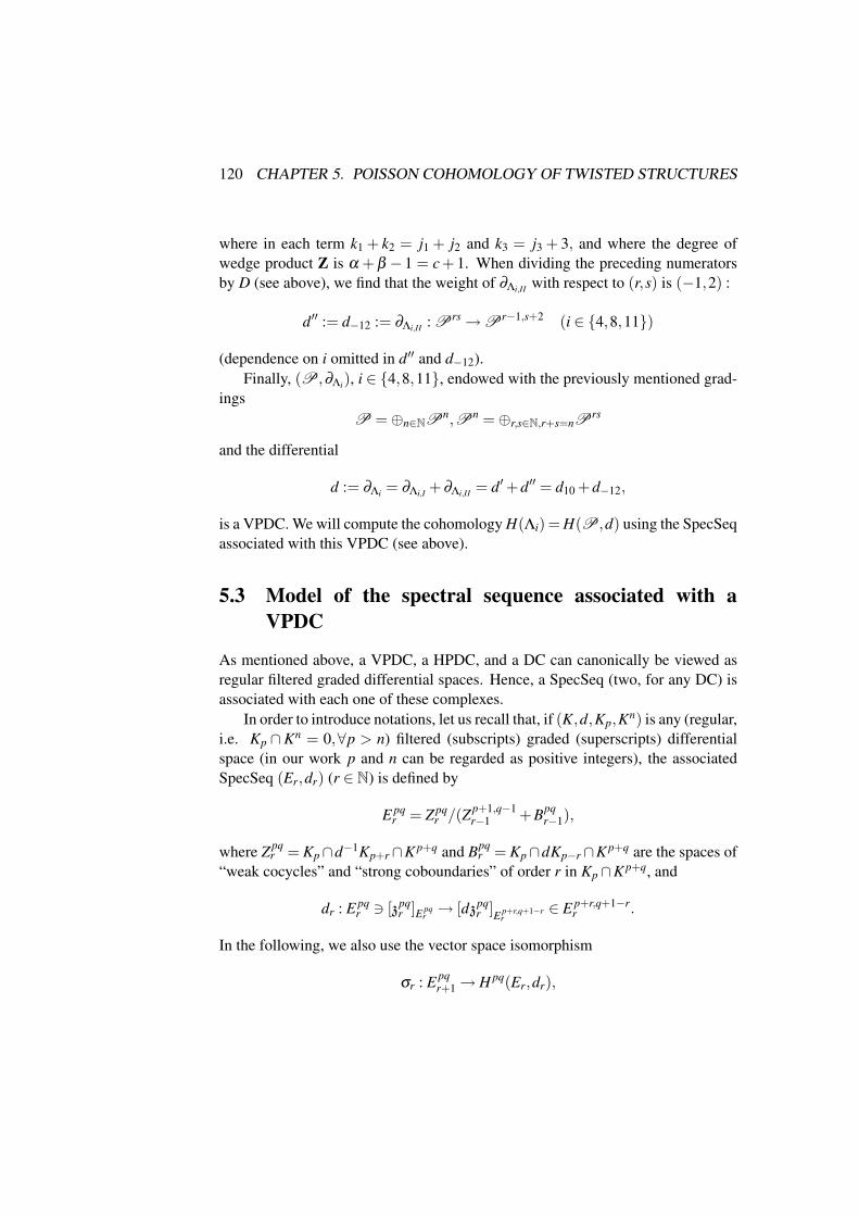
120 CHAPTER 5. POISSON COHOMOLOGY OF TWISTED STRUCTURES
where in each term k1 + k2 = j1 + j2 and k3 = j3 + 3, and where the degree ofwedge product Z is α + β − 1 = c + 1. When dividing the preceding numeratorsby D (see above), we find that the weight of ∂Λi,II with respect to (r,s) is (−1,2) :
d′′ := d−12 := ∂Λi,II : Prs →Pr−1,s+2 (i ∈ 4,8,11)
(dependence on i omitted in d′′ and d−12).Finally, (P,∂Λi), i ∈ 4,8,11, endowed with the previously mentioned grad-
ingsP =⊕n∈NPn,Pn =⊕r,s∈N,r+s=nP
rs
and the differential
d := ∂Λi = ∂Λi,I +∂Λi,II = d′+d′′ = d10 +d−12,
is a VPDC. We will compute the cohomology H(Λi) = H(P,d) using the SpecSeqassociated with this VPDC (see above).
5.3 Model of the spectral sequence associated with aVPDC
As mentioned above, a VPDC, a HPDC, and a DC can canonically be viewed asregular filtered graded differential spaces. Hence, a SpecSeq (two, for any DC) isassociated with each one of these complexes.
In order to introduce notations, let us recall that, if (K,d,Kp,Kn) is any (regular,i.e. Kp ∩Kn = 0,∀p > n) filtered (subscripts) graded (superscripts) differentialspace (in our work p and n can be regarded as positive integers), the associatedSpecSeq (Er,dr) (r ∈ N) is defined by
E pqr = Zpq
r /(Zp+1,q−1r−1 +Bpq
r−1),
where Zpqr = Kp∩d−1Kp+r∩K p+q and Bpq
r = Kp∩dKp−r∩K p+q are the spaces of“weak cocycles” and “strong coboundaries” of order r in Kp∩K p+q, and
dr : E pqr 3 [zpq
r ]E pqr→ [dzpq
r ]E p+r,q+1−rr
∈ E p+r,q+1−rr .
In the following, we also use the vector space isomorphism
σr : E pqr+1 → H pq(Er,dr),

5.3. MODEL OF SPECTRAL SEQUENCES 121
which assigns to each [zpqr+1]E pq
r+1, z
pqr+1 ∈ Zpq
r+1 ⊂ Zpqr , the dr-cohomology class
[[zpqr+1]E pq
r]dr , [zpq
r+1]E pqr∈ E pq
r ∩ kerdr. For more detailed results on spectralsequences, we refer the reader to [Cle85], [God52], [CE56], [Vai73], ... In thesemonographs, a model for the SpecSeq associated with a (HP)DC is partiallydepicted up to r = 2. It is well-known that spectral sequences are particularly easyto use, if many spaces E pq
2 (or E pqr (r > 2)) vanish. Due to richness of Poisson
cohomology, this lacunary phenomenon is less pronounced in our setting. Sincewe have thus to compute through the whole SpecSeq, we need the completedescription of the entire model of the SpecSeq (Er,dr) (r ∈ N) associated with aVPDC.
So consider an arbitrary VPDC and let Gpq(K) (p,q∈N) be the term of degree(p,q) of the bigraded space associated with the filtered graded space K. It is clearthat the mapping
I0 : E pq0 = Kp∩K p+q/Kp+1∩K p+q = Gpq(K)3 [zpq
0 =q
∑i=0
zq−i,p+i]E pq0→ zqp ∈Kqp,
where zrs (as well as—in the following—all Latin characters with double super-script) is an element of Krs (whereas German Fraktur characters with double su-perscript, such as z
pq0 , do not refer to the bigrading of K), is an isomorphism of
bigraded vector spaces (i.e. a vector space isomorphism that respects the bigrad-ing). It is easily seen that, when reading d0 through this isomorphism, we get thecompound map
d0 = I0d0I−10 = d10.
Thus I0 : (E0,d0) → (K,d0) is an isomorphism between bigraded differentialspaces, and induces an isomorphism
I0] : H pq(E0,d0) 3 [[zpq0 = ∑q
i=0 zq−i,p+i]E pq0
]d0
−→ [zqp]d0∈ H pq(K,d0) =: 0H pq(K) = 0Hq(K∗p)
of bigraded vector spaces, where the last space is the q-term of the cohomologyspace of (K∗p,d0 = d10). Hence the bigraded vector space isomorphism
I1 = I0]σ0 : E pq1 3 [zpq
1 =q
∑i=0
zq−i,p+i]E pq1→ [[zpq
1 ]E pq0
]d0 → [zqp]d0∈ 0Hq(K∗p).
We now again verify straightforwardly that differential d1 read on model 0H(K) isinduced by d01, i.e. that
d1 = I1d1I−11 = d01].

122 CHAPTER 5. POISSON COHOMOLOGY OF TWISTED STRUCTURES
Finally,
I2 = I1]σ1 : E pq2 3 [zpq
2 =q
∑i=0
zq−i,p+i]E pq2→ [[zpq
2 ]E pq1
]d1 → [[zqp]d0]d1∈1H p(0Hq(K))
is an isomorphism of bigraded vector spaces. As for the sense of the last space,note that (0Hq(K) =⊕p
0Hq(K∗p),d1) is a complex. Observe now that the inverseI−12 is less straightforward than I−1
0 and I−11 . Indeed, if [[zqp]d0
]d1∈1H p(0Hq(K)),
representative zqp is generally not a member of Zpq2 . However, since the considered
class makes sense,d10zqp = 0d01zqp +d10zq−1,p+1 = 0,
where zq−1,p+1 ∈ Kq−1,p+1. Thus, zpq2 := zqp + zq−1,p+1 ∈ Zpq
2 and
I−12 [[zqp]d0
]d1= [zpq
2 ]E pq2
.
Sod2[[zqp]d0
]d1= I2[dz
pq2 ]E p+2,q−1
2= [[d−12zqp +d01zq−1,p+1]d0
]d1.
The preceding results extend those given in [Vai73] (for a HPDC). They can easilybe adapted to the most frequently encountered situations where only some termsdab of d do not vanish.
In the following, we complete the description of the SpecSeq associated witha VPDC, assuming that d = d10 + d−12 := d′ + d′′. This hypothesis entails thatd′2 = d′′2 = d′d′′+d′′d′ = 0, i.e. that d′ and d′′ are two anticommuting differentials.Hereafter, we denote by rH(.) (r ∈N) the cohomology of differential d2r and by [.]rthe corresponding classes. Moreover, we will deal with strongly triangular systemsof type
d′zqp = 0 (E0)d′′zqp +d′zq−2,p+2 = 0 (E1). . .
d′′zq−2(k−2),p+2(k−2) +d′zq−2(k−1),p+2(k−1) = 0. (Ek−1)
Note that when solving such a system, we prove at each stage that some d′-cocycleis actually a d′-coboundary. We refer to this kind of system using the notationS(zqp;k) or S(k;zq−2(k−1),p+2(k−1)) depending on the necessity to emphasize thefirst or the last unknown or entry of an ordered solution.
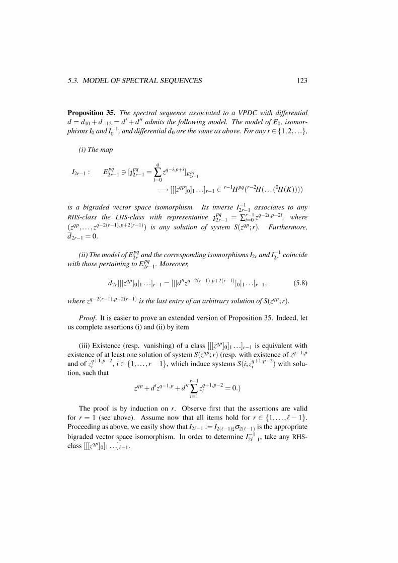
5.3. MODEL OF SPECTRAL SEQUENCES 123
Proposition 35. The spectral sequence associated to a VPDC with differentiald = d10 + d−12 = d′ + d′′ admits the following model. The model of E0, isomor-phisms I0 and I−1
0 , and differential d0 are the same as above. For any r ∈ 1,2, . . .,
(i) The map
I2r−1 : E pq2r−1 3 [zpq
2r−1 =q
∑i=0
zq−i,p+i]E pq2r−1
−→ [[[zqp]0]1 . . .]r−1 ∈ r−1H pq(r−2H(. . .(0H(K))))
is a bigraded vector space isomorphism. Its inverse I−12r−1 associates to any
RHS-class the LHS-class with representative zpq2r−1 = ∑r−1
i=0 zq−2i,p+2i, where(zqp, . . . ,zq−2(r−1),p+2(r−1)) is any solution of system S(zqp;r). Furthermore,d2r−1 = 0.
(ii) The model of E pq2r and the corresponding isomorphisms I2r and I−1
2r coincidewith those pertaining to E pq
2r−1. Moreover,
d2r[[[zqp]0]1 . . .]r−1 = [[[d′′zq−2(r−1),p+2(r−1)]0]1 . . .]r−1, (5.8)
where zq−2(r−1),p+2(r−1) is the last entry of an arbitrary solution of S(zqp;r).
Proof. It is easier to prove an extended version of Proposition 35. Indeed, letus complete assertions (i) and (ii) by item
(iii) Existence (resp. vanishing) of a class [[[zqp]0]1 . . .]r−1 is equivalent withexistence of at least one solution of system S(zqp;r) (resp. with existence of zq−1,p
and of zq+1,p−2i , i ∈ 1, . . . ,r− 1, which induce systems S(i;zq+1,p−2
i ) with solu-tion, such that
zqp +d′zq−1,p +d′′r−1
∑i=1
zq+1,p−2i = 0.)
The proof is by induction on r. Observe first that the assertions are validfor r = 1 (see above). Assume now that all items hold for r ∈ 1, . . . , `− 1.Proceeding as above, we easily show that I2`−1 := I2(`−1)]σ2(`−1) is the appropriatebigraded vector space isomorphism. In order to determine I−1
2`−1, take any RHS-class [[[zqp]0]1 . . .]`−1.

124 CHAPTER 5. POISSON COHOMOLOGY OF TWISTED STRUCTURES
Let us first prove assertion (iii). Existence of class [[[zqp]0]1 . . .]`−1 is equivalentwith existence of class [[[zqp]0]1 . . .]`−2 (itself equivalent to existence of at least onesolution
zq−2 j,p+2 j (0≤ j ≤ `−2)
for S(zqp;`−1), by induction) and condition
d2(`−1)[[[zqp]0]1 . . .]`−2 = 0.
Using the induction assumptions, we see that the last condition is equivalent, firstwith
[[[d′′zq−2(`−2),p+2(`−2)]0]1 . . .]`−2 = 0,
then with existence ofzq−2(`−1),p+2(`−1)
and zq−2(`−2),p+2(`−2)i (1 ≤ i ≤ ` − 2), which implement systems
S(i;zq−2(`−2),p+2(`−2)i ) with solution, say
zq−2 j,p+2 ji (1≤ `− i−1≤ j ≤ `−2),
such that
d′′(
zq−2(`−2),p+2(`−2) +`−2
∑i=1
zq−2(`−2),p+2(`−2)i
)+d′zq−2(`−1),p+2(`−1) = 0. (5.9)
Assume now that all this holds and define new zq−2 j,p+2 j (0≤ j ≤ `−1). For eachj, take just the sum of the old zq−2 j,p+2 j and of all existing zq−2 j,p+2 j
i . These newzq−2 j,p+2 j form a solution of S(zqp;`). Note first that for j ∈ 0, `− 1, the oldand new zq−2 j,p+2 j coincide. Hence, the last equation (E`−1) of S(zqp;`) is nothingbut Equation (5.9). Moreover, it is easily checked that Equations (E`−2), . . . ,(E0)are also verified. Conversely, if S(zqp;`) has a solution, the successive classes[zqp]0, [[zqp]0]1, . . . , [[[zqp]0]1 . . .]`−1 are actually defined. It suffices to note thatd0zqp = 0 and that, by induction,
d2r[[[zqp]0]1 . . .]r−1 = [[[d′′zq−2(r−1),p+2(r−1)]0]1 . . .]r−1
= −[[[d′zq−2r,p+2r]0]1 . . .]r−1 = 0,
for any r ∈ 1, . . . , `−1.

5.4. FORMAL COHOMOLOGY OF POISSON TENSOR Λ4 125
As for the second part of (iii), note that a class [[[zqp]0]1 . . .]`−1 van-ishes if and only if there is zq+2(`−1)−1,p−2(`−1)
`−1 that generates a system
S(zq+2(`−1)−1,p−2(`−1)`−1 ;`−1) with solution, say
zq+2(`− j−1)−1,p−2(`− j−1)`−1 (0≤ j ≤ `−2),
such that
[[[zqp]0]1 . . .]`−2 = −d2(`−1)[[[zq+2(`−1)−1,p−2(`−1)`−1 ]0]1 . . .]`−2
= −[[[d′′zq+1,p−2`−1 ]0]1 . . .]`−2.
But, by induction, [[[zqp + d′′zq+1,p−2`−1 ]0]1 . . .]`−2 = 0 if and only if there are zq−1,p
and zq+1,p−2i (1 ≤ i ≤ `− 2), which induce systems S(i;zq+1,p−2
i ) with solution,such that
zqp +d′′zq+1,p−2`−1 +d′′
`−2
∑i=1
zq+1,p−2i +d′zq−1,p = 0.
Hence the conclusion.
We now revert to items (i) and (ii). For any RHS-class [[[zqp]0]1 . . .]`−1 ∈`−1H pq(`−2H(. . .(0H(K)))), the corresponding system S(zqp;`) admits, as just ex-plained, at least one solution zq−2 j,p+2 j (0≤ j ≤ `−1). Set
zpq2`−1 :=
`−1
∑j=0
zq−2 j,p+2 j.
As dzpq2`−1 = d′′zq−2(`−1),p+2(`−1) ∈ Kq−2`+1,p+2`, we see that z
pq2`−1 ∈ Zpq
2`−1 =Kp ∩ d−1Kp+2`−1 ∩K p+q. Hence I−1
2`−1. As d2`−1[zpq2`−1]E pq
2`−1∈ E p+2`−1,q−2`+2
2`−1 , it
is clear that d2`−1 = 0. Thus, the statement concerning the model of E pq2` and the
isomorphisms I2` and I−12` is obvious. Finally, as d2`[z
pq2` ]E pq
2`∈ E p+2`,q−2`+1
2` , we get
d2`[[[zqp]0]1 . . .]`−1 = [[[d′′zq−2(`−1),p+2(`−1)]0]1 . . .]`−1.
Remark. Result (5.8) can be rephrased as d2r =((−1)r−1d′′(d′−1d′′)r−1
)], for
any r ∈ 1,2, . . ..
5.4 Formal cohomology of Poisson tensor Λ4
As aforementioned, we use the just depicted SpecSeq associated with the abovedetailed VPDC implemented by the twisted r-matrix induced Poisson structure Λ4.

126 CHAPTER 5. POISSON COHOMOLOGY OF TWISTED STRUCTURES
5.4.1 Computation of the second term of the SpecSeq
In this section, we give the second term E2 ' 0H(P) of the SpecSeq. Note that0H(P) is the formal Poisson cohomology of d0 = d′ = d10 = ∂Λ4,I . As alreadyelucidated in the Introduction, we came up with decomposition (5.1), since thecohomology of ∂ΛI is always accessible by the technique proposed in [MP06].Hence, cohomology space 0H(P) can be obtained (quite straightforwardly) by thismodus operandi. Let us emphasize that our results are in accordance, as well withsimilar upshots in [Mon02,2], as with our comments in [MP06], regarding the tightrelation between Casimir functions and Koszul-exactness or “quasi-exactness”, theappearance of “accidental Casimir-like” non bounding cocycles, and the increaseof the “weight in cohomology” of the singularities, with closeness of the consideredPoisson structure to Koszul-exactness.
If ba ∈Q∗, we denote by (β ,α)∼ (b,a), α ∈N∗, the irreducible representative
of ba . Remember that, see [MP06], for b
a ∈Q∗+, a quasi-exact structure
Λ = a∂1(pq)∂23 +a∂2(pq)∂31 +b∂3(pq)∂12, (5.10)
p = p(x,y), q = q(z), exhibits the basic Casimir pαqβ . Furthermore, we set D =xyz, D′ = xy, and write AαY3, α ∈N∗, instead of D′αz−1Y3 = D′α∂3, and ⊕i j . . .Yi j
instead of . . .Y23 + . . .Y31 + . . .Y12. Remark also that the algebra of polynomials ofthe algebraic variety of singularities of Λ4,I is R[[x]]⊕R[[y]]⊕R[[z]], where it isunderstood that term R is considered only once.
The following proposition is now almost obvious.
Proposition 36.
1. If ba ∈ Q∗+, the algebra of Λ4,I-Casimirs is Cas(Λ4,I) = ⊕i∈NRD′αizβ i and
the cohomology space 0H(P)' E2 is given by
0H(P) = Cas(Λ4,I)⊕⊕
i
Cas(Λ4,I)Yi⊕⊕
i j
Cas(Λ4,I)Yi j⊕Cas(Λ4,I)Y123
⊕R[[x]]∂23⊕R[[y]]∂31⊕ (R[[x]]⊕R[[y]])∂123, if b = a0,otherwise
⊕R[[z]]∂12⊕R[[z]]∂123
2. If ba ∈R∗ \Q∗+, we have Cas(Λ4,I) =R and the cohomology space 0H(P)'

5.4. FORMAL COHOMOLOGY OF POISSON TENSOR Λ4 127
E2 is given by
0H(P) = Cas(Λ4,I)⊕⊕
i
Cas(Λ4,I)Yi⊕⊕
i j
Cas(Λ4,I)Yi j⊕Cas(Λ4,I)Y123
⊕RAαY3⊕Aα(RY23 +RY31)⊕RAαY123, if (−1,α)∼ (b,a)0,otherwise
⊕R[[z]]∂12⊕R[[z]]∂123
Remark. Due to the properties—used below—of the preceding (non bound-ing) Λ4,I-cocycles, we classify these representatives as follows:
1. Representatives of type 1: All cocycles with cochain degree 0, the 1− and2−cocycles that contain a Casimir (maybe the accidental Casimir Aα ), ex-cept cocycles Cas(Λ4,I)Y12
2. Representatives of type 2: All 3−cocycles, all cocycles with singularities,and cocycles Cas(Λ4,I)Y12
5.4.2 Prolongable systems S(zqp;r)
Since computation through the whole SpecSeq will shape up as inescapable, weneed the below corollary of Proposition (35). It allows to short-circuit the pro-cess of computing the successive terms of the sequence. Let us specify that in thefollowing a system of representatives of a space of classes is made up by represen-tatives that are in 1-to-1 correspondence with the considered classes.
Corollary 4. If, for some fixed r ∈ N∗, all the classes [[[zqp]0]1 . . .]r−1 in modelspace r−1H(r−2H(. . .0H(K))), appendant on a SpecSeq associated to a VPDC withdifferential d = d10 +d−12 = d′+d′′, give rise to an enlarged system S(zqp;s) withsolution, for some fixed s≥ r, the following upshots hold:
1. All the differentials d2r−1,d2r, . . . ,d2s−1 vanish
2. Differential d2s is defined by
d2s[[[zqp]0]1 . . .]r−1 = [[[d′′zq−2(s−1),p+2(s−1)]0]1 . . .]r−1
3. Any system (zqp) of representatives of r−1H(r−2H(. . .0H(K))) is in 1-to-1correspondence with the system (zpq
2s := ∑s−1k=0 zq−2k,p+2k) of representatives
of E2s
Proof. Induction on s.

128 CHAPTER 5. POISSON COHOMOLOGY OF TWISTED STRUCTURES
5.4.3 Forecast
In order to increase readability of this chapter, some intuitive advisements are nec-essary.
The basic idea of the theory of spectral sequences is that computation of thesuccessive terms Er ' H(Er−1,dr−1) (r ∈ N∗) allows to detect their inductive limitE∞, which—for a convergent sequence—is isomorphic with the graded space G(H)associated to the sought-after filtered cohomology space H. We then hope tobe able to reconstruct this filtered space H from the corresponding graded spaceG(H). Let us recall that space H is of course the cohomology of the filtered gradeddifferential space associated with the SpecSeq. Hence, in our case, H = H(Λ4).It is clear that the successive cohomology computations take place on the concretemodel side. To determine H, we have to pull our results back to the theoretical side,and more precisely to read them through the numerous isomorphisms involved.
Actually the application of spectral sequences presented in this work, providesa beautiful insight into the operating mode of a SpecSeq. Since—roughly spoken—the “weak cocycle condition” in the definition of Zpq
r (resp. the “strong coboundarycondition” in the definition of Bpq
r ) converges to the usual cocycle condition (resp.the usual coboundary condition), we understand that, when passing from one es-timate Er−1 of H to the next approximation Er, we obtain an increasing numberof conditions on our initial weak non bounding cocycles of E2 and an increasingnumber of bounding cocycles. Moreover, when we compute through the SpecSeq,the aforementioned pullbacks, see Proposition (35), add up solutions of crescivesystems,
zpq2r = zqp +
r−1
∑k=1
zq−2k,p+2k.
The next remarks aim at anticipation of these systems. The reader is alreadyfamiliar with Casimirs of exact and quasi-exact structures. When taking an interestin slightly more general quasi-exact tensors,
Λ = a∂1((p+ r)q)∂23 +a∂2((p+ r)q)∂31 +b∂3((p+ r)q)∂12, (5.11)
a,b ∈ R∗, p = p(x,y), q = q(z), r = r(z), it is natural to ask which polynomials ofthe type (p+ cr)nqm, c ∈ R, n,m ∈ N, (n,m) 6= (0,0), are Casimir functions. It iseasily checked that structure Λ4 has this form and that the Casimir conditions readam = bn and 3bn = ca(2n+m). So, for b
a ∈Q∗+, the basic Casimir C of Λ4 and its

5.4. FORMAL COHOMOLOGY OF POISSON TENSOR Λ4 129
powers Ci, i ∈ N, are given by
Ci = (p+3b
2a+br)α iqβ i = (D′+
z2
2a+b)α izβ i
= D′α izβ i +α i
∑k=1
kα i
(2a+b)k D′α i−kzβ i+2k.
These powers Ci (non bounding cocycles of H = H(Λ4)) will be obtained—whilewe compute through the SpecSeq—from those, D′α izβ i, of the Casimir of Λ4,I
(non bounding cocycles of E2 ' 0H(P)). Hence, the above-quoted solutions andcorresponding systems S(D′α izβ i,α i+1).
5.4.4 Computation through the SpecSeq
In view of the preceding awareness, it is natural to set
Zqic−2k,pi+2k =k
αi(2a+b)k D′αi−kzβ i+2k
Aik
BikY1 +CikY2 +DikY3 ,
EikY23 +FikY31
where k ∈ 0,1, . . . ,α i and Aik,Bik,Cik,Dik,Eik,Fik ∈ R. More precisely, if ba ∈
Q∗+, we have (b,a) ∼ (β ,α), α,β ∈ N∗, and we ask that i ∈ N, if ba ∈ R∗ \Q∗+,
we choose i = 0, and if moreover (b,a) ∼ (β ,α) = (−1,α), α ∈ N∗, we alsoaccept the value i = 1, but add the conditions A10 = B10 = C10 = 0. We define(qic, pi) := (2α i + 2 + c,β i + 1), where c ∈ 0,1,2 denotes the cochain degree,so that the double superscript in the LHS is the bidegree (r,s) = ( j1 + j2 + c, j3) ofthe RHS.
Observe that the Zqic,pi are exactly the representatives of type 1 of the classesof E2 ' 0H(P).
Lemma 7. For any admissible exponent i and any cochain degree c ∈ 0,1,2,the cochains Zqic−2k,pi+2k, k ∈ 0,1, . . . ,α i, constitute a solution of systemS(Zqic,pi ;α i+1), if and only if, for any k ∈ 0,1, . . . ,α i−1,
Ai,k+1 = Aik, if c = 0, (C0)
Bi,k+1 +Ci,k+1 =(αi− k +1)(Bik +Cik)−2Dik
αi− kand Di,k+1 = Dik, if c = 1, (C1)
Ei,k+1−Fi,k+1 =αi− k +1
αi− k(Eik−Fik) , if c = 2. (C2)

130 CHAPTER 5. POISSON COHOMOLOGY OF TWISTED STRUCTURES
Furthermore,
d′′Zqic−2αi,pi+2αi = d′′Z2+c,pi+2αi
=
0, for c = 0,
(2a+b)−αi (Bi,αi +Ci,αi−2Di,αi)z2+i(2α+β )∂12, for c = 1,
(2a+b)−αi (Ei,αi−Fi,αi)z3+i(2α+β )∂123, for c = 2,
is a d′-coboundary if and only if the coefficient vanishes.
Proof. We must compute the differentials d′ = ∂Λ4,I = [Λ4,I, .] and d′′ = ∂Λ4,II =[D−1z3Y12, .] =: [ f X, .] on the Zqic−2k,pi+2k. These cochains have the form gY :=D−1XJY := D−1D′nzm ∑ j r jY j, n,m ∈ N,r j ∈ R, where the degree c of wedgeproduct Y j is independent of j. Hence, Equation (5.7) gives
d′′(gY ) = [ f X,gY ] = f [X,g]∧Y +(−1)cg[Y , f ]∧X.
On the other hand, Equations (5.5) and (5.6) entail d′(gY ) = [Λ4,I,gY ] =[Λ4,I,g] ∧ Y = ∑` X`(g) Y` ∧ Y , where X1 = bY2 − aY3,X2 = aY3 − bY1,X3 =a(Y1−Y2). Since
Y`
(XJ
D
)= ( j`−1)
XJ
D
(same notations as above), we get
d′(gY ) = g(b(n−1)−a(m−1))(Y1−Y2)∧Y .
In particular, we recover the result d′Zqic,pi = ig(bα−aβ )(Y1−Y2)∧Y = 0, and,when setting a = 0,b = 1,Y = 1, we find
[X,g] = g(n−1)(Y1−Y2).
We now compute d′′Zqic−2k,pi+2k, k∈ 0,1, . . . ,α i, and d′Zqic−2(k+1),pi+2(k+1),k ∈ 0,1, . . . ,α i−1.
1. c = 0It follows from the preceding equations that
d′′Zqi0−2k,pi+2k = kαi(α i− k)Aik(2a+b)−kD−1D′αi−kz3+β i+2k(Y1−Y2)

5.4. FORMAL COHOMOLOGY OF POISSON TENSOR Λ4 131
and that
d′Zqi0−2(k+1),pi+2(k+1) =−k+1αi (k+1)Ai,k+1(2a+b)−kD−1D′αi−kz3+β i+2k(Y1−Y2).
Since for any p,n ∈ N, p < n, we have pn(n− p) = p+1
n (p + 1), the sum of thesecoboundaries vanishes if and only if Ai,k+1 = Aik, for any k ∈ 0,1, . . . ,α i− 1.For k = α i, we get
d′′Zqi0−2αi,pi+2αi = d′′Z2,pi+2αi = 0.
2. c = 1A short computation shows that
d′′Zqi1−2k,pi+2k
= kαi(2a+b)−kD−1D′αi−kz3+β i+2k[−Dik(α i− k)Y23−Dik(α i− k)Y31
+((Bik +Cik)(α i− k +1)−2Dik)Y12]
and that
d′Zqi1−2(k+1),pi+2(k+1)
=−k+1α i (k +1)(2a+b)−kD−1D′α i−kz3+β i+2k[−Di,k+1Y23
−Di,k+1Y31 +(Bi,k+1 +Ci,k+1)Y12].
If k ∈ 0,1, . . . ,α i−1, the sum of these coboundaries vanishes if and only if
Bi,k+1 +Ci,k+1 =(αi− k +1)(Bik +Cik)−2Dik
αi− kand Di,k+1 = Dik.
Furthermore, for k = α i, the first of the preceding “coboundary equations”provides the announced result for d′′Zqi1−2αi,pi+2αi. As R[[z]]∂12 is part of thecohomology of d0 = d′, this d′′-coboundary is a d′-coboundary if and only if itscoefficient vanishes.
3. c = 2We immediately obtain
d′′Zqi2−2k,pi+2k = kαi(α i− k +1)(2a+b)−kD−1D′αi−kz3+β i+2k(Eik−Fik)Y123
and
d′Zqi2−2(k+1),pi+2(k+1)
=−k+1αi (k +1)(2a+b)−kD−1D′α i−kz3+β i+2k(Ei,k+1−Fi,k+1)Y123.

132 CHAPTER 5. POISSON COHOMOLOGY OF TWISTED STRUCTURES
Hence the announced upshots.Let us recall that the admissible values of i (and the potential conven-
tions on coefficients A10,B10,C10) depend on quotient b/a. Moreover, for b/a ∈ R∗ \Q∗+,(b,a) (−1,α),α ∈ N∗, we set α = 1 ∈ N∗. Actually, in this case,α needed not be defined before, as it was systematically multiplied by i = 0.
The following theorem provides the complete description of the consideredSpecSeq.
Theorem 18. The even terms E2(n−1)α+4 = E2(n−1)α+6 = . . . = E2nα+2 (n ∈ N;for n = 0, this package contains only term E2) of the above defined SpecSeq arecanonically isomorphic (i.e. d2(n−1)α+4 = d2(n−1)α+6 = . . . = d2nα = 0 ) and admitthe below system of representatives:1. All representatives of type 2 of E2 ∼ 0H(P), except
Rzi(2α+β )+2∂12 and Rzi(2α+β )+3∂123,
for all admissible i ∈ 0,1, . . . ,n−1.2. All representatives of type 1 of E2 ∼ 0H(P), altered as follows:
• For all admissible i ∈ n,n+1, . . .,
Zqic,pi Ãα n
∑k=0
Zqic−2k,pi+2k,
where the coefficients Aik,Bik,Cik,Dik,Eik,Fik incorporated into the terms ofthe RHS verify conditions (C0)− (C2) of Lemma 7 up to k = α n−1.
• For all admissible i ∈ 0,1, . . . ,n−1,
Zqic,pi Ã
(D′+ z2
2a+b
)αizβ iAi0, if c = 0,
(D′+ z2
2a+b
)αizβ i
(Bi0(Y1 + 1
2Y3)+Ci0(Y2 + 12Y3)
), if c = 1,
D′αizβ iEi0(Y23 +Y31), if c = 2.
Proof. The proof is by induction on n. For n = 0, Theorem 18 is obviouslyvalid. Assume now that it holds true for 0,1, . . . ,n− 1 (n ∈ N∗). We first transferthe description of E2(n−2)α+4 = . . . = E2(n−1)α+2 to the concrete model side, inorder to compute d2(n−1)α+2. When having a look at the packages of terms that areknown to be isomorphic, we see that the only differentials (under d2(n−1)α+2) that

5.4. FORMAL COHOMOLOGY OF POISSON TENSOR Λ4 133
do not vanish are d2mα+2 (m ∈ 0,1, . . . ,n−2). Hence the target of vector spaceisomorphism
I2(n−1)α+2 : E2(n−1)α+2 → (n−2)α+1H((n−3)α+1H(. . .1H(0H(P)))),
which—as it appears from its general description—maps the system of E2(n−1)α+2-representatives onto the system evidently made up by:
1. All representatives of type 2 of E2, except Rzi(2α+β )+2∂12 andRzi(2α+β )+3∂123, for all admissible i ∈ 0,1, . . . ,n−2.
2. All representatives of type 1 of E2, Zqic,pi , i admissible, c∈0,1,2, with, forall admissible i ∈ 0,1, . . . ,n−2, Bi0 +Ci0 = 2Di0, if c = 1, and Ei0 = Fi0,if c = 2.
We now compute the cohomology of space
((n−2)α+1H(. . .0H(P)),d2(n−1)α+2).
If zqp is one of the representatives of the preceding system,
d2(n−1)α+2[[zqp]0 . . .](n−2)α+1 = [[d′′zq−2α(n−1),p+2α(n−1)]0 . . .](n−2)α+1, (5.12)
where zq−2α(n−1),p+2α(n−1) is the last entry of an arbitrary solution of S(zqp;α(n−1)+1).
The d′′-coboundary of any zqp of type 2 vanishes. This is obvious if zqp is a 3-cochain or has the form Cas(Λ4,I)Y12 (as d′′ = [Λ4,II, .] = [D−1z3Y12, .]). If zqp is a 2-cochain with singularities, e.g. D−1 p(x)Y23, where p(x) is a polynomial in x, we getd′′zqp = [D−1z3Y12,D−1 p(x)Y23] = −z3 p(x)D−2Y123 + z3 p(x)D−2Y123 = 0. Hence,for any type 2 representative zqp, system S(zqp;s) admits solution (zqp,0, . . . ,0), forany s ∈ N∗ (S1, representative extended by 0 [reference needed in the following]),and Coboundary (5.12) vanishes.
Let now zqp be a representative Zqic,pi of the first type. We know from Lemma7 that Zqic−2k,pi+2k, k ∈ 0,1, . . . ,α i, with coefficients that verify (C0)-(C2), is asolution of S(Zqic,pi ;α i+1).
1. For any admissible i ∈ n,n + 1, . . ., this solution can be truncated to asolution of S(Zqic,pi ;α n+1) (S2, truncated standard solution). Hence, Coboundary(5.12) vanishes.

134 CHAPTER 5. POISSON COHOMOLOGY OF TWISTED STRUCTURES
2. If i is admissible in 0,1, . . . ,n−2, we have
Bi0 +Ci0 = 2Di0 and Ei0 = Fi0.
It then follows from (C1) and (C2) that the same relation holds for k = α i,i.e. that Bi,α i + Ci,α i = 2Di,α i and Ei,α i = Fi,α i. This however implies thatd′′Zqic−2α i,pi+2α i = 0, so that system S(Zqic,pi ;α n+1) admits an obvious solution(S3, standard solution extended by 0) and that Coboundary (5.12) vanishes again.
3. If i = n−1 is admissible,
d2(n−1)α+2[[Zqn−1,c,pn−1 ]0 . . .](n−2)α+1
= [[d′′Zqn−1,c−2α(n−1),pn−1+2α(n−1)]0 . . .](n−2)α+1.
In view of Lemma 7, this class vanishes for c = 0, and coincides, if c = 1(resp. c = 2), up to a coefficient, with class [[z(n−1)(2α+β )+2∂12]0 . . .](n−2)α+1
(resp. [[z(n−1)(2α+β )+3∂123]0 . . .](n−2)α+1). The above depicted system of repre-sentatives of (n−2)α+1H(. . .0H(P)) shows that the preceding two classes do notvanish. Hence, the cocycle-condition is equivalent with the annihilation of thementioned coefficient, i.e. with
Bn−1,α(n−1) +Cn−1,α(n−1) = 2Dn−1,α(n−1) (resp. En−1,α(n−1) = Fn−1,α(n−1)),
or, as already explained,
Bn−1,0 +Cn−1,0 = 2Dn−1,0 (resp. En−1,0 = Fn−1,0). (5.13)
Since it clearly follows from our computations that the spaceof d2(n−1)α+2-coboundaries is generated by the two just encoun-tered non-vanishing classes, cohomology space (n−1)α+1H((n−2)α+1H(. . .0H(P))) has the same system of representatives than its predecessor(n−2)α+1H(. . .0H(P)), but with exclusions carried out and conditions onBi0,Ci0,Di0,Ei0,Fi0 valid for all admissible i ∈ 0,1, . . . ,n−1.
It now suffices to apply Corollary 4 to cohomology space(n−1)α+1H((n−2)α+1H(. . .0H(P))). Observe first that (S1)-(S3) entail exis-tence of a solution of S(zqp;α n + 1), for all representatives zqp dissimilar fromZqn−1,c,pn−1 . But, as the coefficients of these last representatives—viewed as rep-resentatives of the preceding d2(n−1)α+2-cohomology space—satisfy Conditions

5.4. FORMAL COHOMOLOGY OF POISSON TENSOR Λ4 135
(5.13), the coboundaries d′′Zqn−1,c−2α(n−1),pn−1+2α(n−1) vanish. So the previouslymet solution of S(Zqn−1,c,pn−1 ;α (n−1)+ 1) can be indefinitely extended by 0 (S4,standard solution extended by 0). Finally, Corollary 4 is applicable for s = α n+1.
Hence, spaces E2(n−1)α+4 = . . . = E2nα+2 coincide and we build, from theknown system zqp of representatives of (n−1)α+1H(. . .0H(P)), a system of E2nα+2by just summing-up the entries of any solutions of the systems S(zqp;α n+1). Forany Zqic,pi , the coefficients of which verify
Bi0 +Ci0 = 2Di0 (c = 1) and Ei0 = Fi0 (c = 2),
the standard Zqic−2k,pi+2k, k ∈ 0,1, . . . ,α i, are solution, see Lemma 7, ofS(Zqic,pi ;α i+1), e.g. if we choose
Aik = Ai0 (c = 0), Bik = Bi0, Cik = Ci0,Dik = Di0 (c = 1), and Eik = Fik = 0 (c = 2,k 6= 0).
(5.14)
If we pull the concrete side representatives back to theoretical side representativesusing these solutions, we exactly get, see S1-S4, the sought-after system.
Remark.
1. We already observed previously the obvious fact that when pulling RHS-representatives back, using different solutions of the standard system, we ob-tain equivalent LHS-representatives. These equivalent LHS-representativeswould implement cohomologous cocycles in cohomology space H(Λ4).Choice (5.14) will induce in cohomology the most basic possible cocycles.
2. Note also that in view of Theorem 18 and our conventions on coefficientsB10,C10, cocycle RAαY3 disappears from all spaces E2r, r ≥ 2α +4.
5.4.5 Limit of the SpecSeq and reconstruction of the cohomology
The limit of the SpecSeq can be guessed from Theorem 18. However, we alreadystressed the importance of a careful reading of all results through the isomorphismsinvolved in the theory of spectral sequences. The proof of Theorem 18 shows forinstance that the appropriate Casimir functions appear, when we pull the RHS-representatives back to the LHS, i.e. read them through isomorphism I−1
2(n−1)α+3.Hence, a precise description of the isomorphisms that lead now to the cohomologyof Λ4 is essential.

136 CHAPTER 5. POISSON COHOMOLOGY OF TWISTED STRUCTURES
General results
Let us consider the SpecSeq associated with a (regular) filtered graded differentialspace (K,d,Kp,Kn) and recall that the limit spaces E pq
∞ ,Zpq∞ ,Bpq
∞ are defined ex-actly as spaces E pq
r ,Zpqr ,Bpq
r , see Section 5.3, so that Zpq∞ and Bpq
∞ are the spacesof cocycles and coboundaries in Kp ∩K p+q respectively. For any fixed p and q,regularity implies that the target space of the restriction of dr to E pq
r vanishes, ifr > q+1. Thus, there is a canonical linear surjective map
ϑ pqr : E pq
r → H pq(Er,dr)→ E pqr+1.
For s≥ r > q+1, we define θ pqrs := ϑ pq
s−1 . . .ϑ pqr : E pq
r → E pqs , and for r > q+1,
we setθ pq
r : E pqr 3 [zpq
r ]E pqr→ [zpq
r ]E pq∞ ∈ E pq
∞ . (5.15)
Due to regularity, the first two of the well-known inclusions Zpq∞ ⊂ Zpq
r ,Zp+1,q−1∞ ⊂
Zp+1,q−1r−1 , and Bpq
r−1 ⊂ Bpq∞ are actually double inclusions, and Zp+1,q−1
∞ + Bpqr−1 ⊂
Zp+1,q−1∞ + Bpq
∞ ⊂ Zpq∞ . Hence, map θ pq
r is canonical, linear and surjective. It isknown that space E pq
∞ together with the preceding linear surjections θ pqr is a model
of the inductive limit of the inductive system (E pqr ,θ pq
rs ). Consider now a first quad-rant SpecSeq (i.e. p,q ∈ N) and assume that K0 = K. For any p,q, the SpecSeqcollapses at
r > sup(p,q+1),
more precisely, E pqr = E pq
∞ and θ pqr = id. Indeed, in this case, in addi-
tion to the aforementioned double inclusions (r > q + 1), we now have alsoBpq
r−1 = Kp ∩ dKp+1−r ∩ K p+q = Kp ∩ dK0 ∩ K p+q = Bpq∞ (r > p). Hence the
announced results.
The SpecSeq associated with any filtered graded differential space is conver-gent in the sense that limit E pq
∞ is known to be isomorphic as a vector space withterm Gpq of the bigraded space G(H(K)), G for short, associated with the filteredgraded space H(K). Let us recall that the filtration of H(K) is induced by that of K.More precisely, injection i : (Kp,d)→ (K,d) is a morphism of differential spacesand Hp := i]H(Kp)⊂H(K) is the mentioned filtration of H(K). In order to reducenotations, we denote the terms of the grading of H(K) simply by Hn. It is a fact thatthe filtration and the grading of H(K) are compatible and that filtration Hp is regu-lar if its generatrix Kp is. Hence, Hp = ⊕q∈NHp∩H p+q =: ⊕q∈NH p+q
p . Finally, itis a matter of knowledge that the isomorphism, say ι , between Gpq := H p+q
p /H p+qp+1
and E pq∞ is canonical,
ι : E pq∞ 3 [zpq
∞ ]E pq∞ → [[zpq
∞ ]H p+qp
]Gpq ∈ Gpq. (5.16)

5.4. FORMAL COHOMOLOGY OF POISSON TENSOR Λ4 137
We now reconstruct H(K) from G. Let us again focus on a first quadrant Spec-Seq associated with a (regular) filtered complex (K,d,Kp,Kn) (such that K0 = K).For any n ∈ N, we denote by Gn− j1, j1 ,Gn− j2, j2 , . . . ,Gn− jkn , jkn , n ≥ j1 > j2 > .. . >jkn ≥ 0, the non vanishing Gpq = H p+q
p /H p+qp+1 , p + q = n. Since H0 = H(K) and
Hnp = Hp∩Hn = 0,∀p > n, it follows that
Hn = Hn0 = . . . = Hn
n− j1 ⊃ Hnn− j1+1 = . . . = Hn
n− j2
⊃ Hnn− j2+1 . . .Hn
n− jkn⊃ Hn
n− jkn+1 = . . . = Hnn = 0.
Hence,
Hn/Hnn− j2 = Gn− j1, j1 , . . . ,Hn
n− jkn−1/Hn
n− jkn= Gn− jkn−1, jkn−1 ,Hn
n− jkn= Gn− jkn , jkn .
However, if B/A = C, A a vector subspace of B, the sequence 0 → A i→ Bp→
C → 0, is a short exact sequence of vector spaces. A short exact sequence in acategory is split if and only if kernel A admits in vector space B a complementarysubspace that is a subobject, or—alternatively—if and only if there is a right inversemorphism χ : C → B of projection p. Of course, in the category of vector spacessuch a sequence is always split. If χ is a linear right inverse of p, we have B =A⊕χ(C).
Let us now come back to our circumstances. If χ1, . . . ,χkn−1 denote splittingsof the involved sequences, central extension Hn is given by
Hn = χ1(Gn− j1, j1)⊕ . . .⊕χkn−1(Gn− jkn−1, jkn−1)⊕Gn− jkn , jkn . (5.17)
It follows of course from Equation (5.17) that H(K) is—in this vector spacesetting—isomorphic with G = G(H(K)). It is known that in the case of ring coeffi-cients, extension problems may prevent the reconstruction of H(K) from G(H(K)).
Application to Poisson tensor Λ4
The next proposition provides a system of representatives of the cohomology spaceof
Λ4 = ayz∂23 +axz∂31 +(bxy+ z2)∂12 (a 6= 0,b 6= 0).
Remember that D′ = xy and Y1 = x∂1,Y2 = y∂2,Y3 = z∂3. If ba ∼ β
α ∈Q∗+, we define
Cas(Λ4) :=⊕i∈NR(
D′+z2
2a+b
)α i
zβ i
and use the above introduced notation Cas(Λ4,I) =⊕i∈NRD′α izβ i. If ba ∈R∗ \Q∗+,
we set Cas(Λ4) := R and, as aforementioned, Aα = D′αz−1.

138 CHAPTER 5. POISSON COHOMOLOGY OF TWISTED STRUCTURES
Theorem 19. 1. If ba ∈Q∗+, the cohomology of Λ4 is given by
E∞ ∼ G∼ H(Λ4) =
Cas(Λ4)⊕Cas(Λ4)(Y1 +12
Y3)⊕Cas(Λ4)(Y2 +12
Y3)
⊕Cas(Λ4,I)(Y23 +Y31)⊕Cas(Λ4,I)Y12⊕Cas(Λ4,I)Y123
⊕⊕
k∈N\N(2α+β )+2
Rzk∂12⊕⊕
k∈N\N(2α+β )+3
Rzk∂123
⊕R[[x]]∂23⊕R[[y]]∂31⊕ (R[[x]]⊕R[[y]])∂123, if b = a0,otherwise
2. If ba ∈ R∗ \Q∗+, we have :
E∞ ∼ G∼ H(Λ4) =
Cas(Λ4)⊕Cas(Λ4)(Y1 +12
Y3)⊕Cas(Λ4)(Y2 +12
Y3)
⊕Cas(Λ4)(Y23 +Y31)⊕Cas(Λ4)Y12⊕Cas(Λ4)Y123
⊕ ⊕RAα(Y23 +Y31)⊕RAαY123, if (b,a)∼ (−1,α)
0,otherwise
⊕⊕
k∈N\2,2α+1Rzk∂12⊕⊕k∈N\3,2α+2Rzk∂123, if (b,a)∼ (−1,α)
⊕k∈N\2Rzk∂12⊕⊕
k∈N\3Rzk∂123,otherwise
Proof. Fix a,b ∈R∗ and take any representative of E2. Remember that the rep-resentatives of type 1 are exactly the cochains Zqic,pi (i admissible, c ∈ 0,1,2).Moreover, we say that a representative of type 2 is critical if it has the formRzi(2α+β )+2∂12 or Rzi(2α+β )+3∂123 (i admissible). If the considered representativezqp is of type 2 and not critical (resp. of type 2 and critical, of type 1), we choosen ∈ N such that 2nα + 2 > sup(p,q + 1) (resp. 2nα + 2 > sup(p,q + 1,2iα + 2)[hence, we have n− 1 ≥ i], 2nα + 2 > sup(pi,qic + 1,2iα + 2)). The system ofrepresentatives of E∞ ∼ G specified in Theorem 19 arises now from Theorem 18and from the canonical isomorphisms (5.15) (condition: r > sup(p,q + 1)) and(5.16). These representatives are representatives of bases of the non vanishingGpq. In order to compute H(K), it suffices to build arbitrary splittings in keepingwith Equation (5.17). Hence, it suffices to choose, for any class of any basis of theconcerned Gpq, an arbitrary representative, e.g. the aforementioned one. It followsthat H(K) admits exactly the same representatives as E∞ ∼ G.

5.5. FORMAL COHOMOLOGY OF POISSON TENSOR Λ8 139
Remarks. Hence, the twist makes a threefold impact on cohomology. Whenapplying our computing device, see Theorem 18, we get, at each turn of the han-dle, on the model level, roughly speaking, cocycle-conditions on the coefficientsrelated with an additional power of the basic Casimir CΛ4,I of Λ4,I , and we excludea supplementary pair of singularity-induced classes. These conditions appear incohomology as terms Yi or Yi j with the same “Casimir-coefficient”. Eventually, thecocycle-conditions allow to lift the mentioned accessory power of CΛ4,I to the reallevel as power of Casimir CΛ4 of Λ4 or—depending on cochain degree—as powerof Casimir CΛ4,I . We know that such a lift is not unique and that two differentones are cohomologous. It follows from Theorem 19 (resp. from the proof ofTheorem 18) that any term of Cas(Λ4)(Y23 +Y31) is a Λ4-cocycle (resp. can bechosen as lift of the corresponding term in Cas(Λ4,I)(Y23 +Y31), as well as thisterm itself). So any term of Cas(Λ4)(Y23 +Y31) is cohomologous to the analogousterm in Cas(Λ4,I)(Y23 +Y31). Finally, the aforementioned proof allows to see thatΛ4,I-cocycle RAαY3 = RD′αz−1Y3, which is not a product of two Λ4-cocycles, is aΛ4-cocycle if and only if its coefficient vanishes.
Let us in the end have a look at singularities. The singular locus of Λ4,I (resp.Λ4) is made up by the three coordinate axes (resp. the axis of abscissæ and the axisof ordinates). Comparing the results of Proposition 36 and of Theorem 19, we seethat the twist Λ4,II , which removes the z-axis from the singular locus, cancels onlypart of the corresponding polynomials in cohomology. We already observed in[MP06] that, for r-matrix induced tensors, some coefficients of non bounding 2- or3-cocycles can just be interpreted as polynomials on singularities via an extensionof the polynomial ring of the singular locus. In the case of twisted r-matrix inducedstructures, some of these polynomial coefficients are simply not polynomials onsingularities.
5.5 Formal cohomology of Poisson tensor Λ8
We now describe the cohomology space of the twisted quadratic Poisson structure
Λ8 =(
a+b
2(x2 + y2)± z2
)∂12 +axz∂23 +ayz∂31 (a 6= 0,b 6= 0).
If we substitute c (resp. b) for −b (resp. (a+b)/2), tensor Λ8 reads
Λ8 = b(x2 + y2)∂12 +(2b+ c)xz∂23 +(2b+ c)yz∂31± z2∂12. (5.18)

140 CHAPTER 5. POISSON COHOMOLOGY OF TWISTED STRUCTURES
Henceforth we use parameters b and c. Assumptions a 6= 0,b 6= 0 areequivalent with 2b + c 6= 0,c 6= 0. Moreover, the r-matrix induced partΛ8,I = b(x2 + y2)∂12 +(2b+ c)xz∂23 +(2b+ c)yz∂31 of Λ8 is nothing but structureΛ7 with parameter a = 0, see [MP06, Section 9], so that term E2 ' H(Λ8,I) of thespectral sequence follows from [MP06, Theorems 6,8,9].
Let us recall that the Yi stem from Λ8,I , i.e. from Λ7. Hence, Y1 = x∂1 +y∂2,Y2 = x∂2− y∂1,Y3 = z∂3. We set D′ = x2 + y2. Moreover, if b
c ∈ Q,b(2b +c) < 0, we denote by (β ,γ) ∼ (b,c) the irreducible representative of the rationalnumber b
c , with positive denominator, β ∈ Z,γ ∈ N∗, and if bc ∈Q,b(2b + c) > 0,
(β ,γ) ∼ (b,c) denotes the irreducible representative with positive numerator, β ∈N∗,γ ∈ Z∗.
Theorem 20. The terms of the cohomology space of Λ8 (see (5.18)) are given bythe following equations:
1. If bc ∈Q,b(2b+ c) > 0,
H0(Λ8) = Cas(Λ8) =⊕i∈N,γi∈2ZR(
D′± z2
3b+ c
)(β+ γ2 )i
zβ i ,
H1(Λ8) = Cas(Λ8,I)Y2⊕Cas(Λ8)(Y1 +Y3) ,
H2(Λ8) = Cas(Λ8,I)Y12⊕Cas(Λ8,I)Y23⊕⊕
k∈N\N(3β+γ)+2
Rzk∂12 ,
H3(Λ8) = Cas(Λ8,I)Y123⊕⊕
k∈N\N(3β+γ)+3
Rzk∂123 ,
where Cas(Λ8,I) =⊕i∈N,γi∈2ZRD′(β+ γ2 )izβ i.

5.5. FORMAL COHOMOLOGY OF POISSON TENSOR Λ8 141
2. If bc /∈Q or b
c ∈Q,b(2b+ c) < 0,
H0(Λ8) = Cas(Λ8) = R ,
H1(Λ8) = Cas(Λ8)Y2⊕Cas(Λ8)(Y1 +Y3) ,H2(Λ8) = Cas(Λ8)Y12⊕Cas(Λ8)Y23
⊕⊕
k∈N\2,γ−1Rzk∂12, if (b,c)∼ (−1,γ), γ ∈ 4,6,8, ...⊕
k∈N\2Rzk∂12,otherwise
⊕RAγY23, if (b,c)∼ (−1,γ),γ ∈ 4,6,8, ...0,otherwise ,
H3(Λ8) = Cas(Λ8)Y123
⊕⊕
k∈N\3,γRzk∂123, if (b,c)∼ (−1,γ),γ ∈ 4,6,8, ...⊕
k∈N\3Rzk∂123,otherwise
⊕RAγY123, if (b,c)∼ (−1,γ),γ ∈ 4,6,8, ....0,otherwise ,
where Aγ = D′ γ2−1z−1.
3. If b = 0,
H0(Λ8) = Cas(Λ8) =⊕i∈NR(
D′± z2
c
)i
,
H1(Λ8) = Cas(Λ8,I)Y2⊕Cas(Λ8)(Y1 +Y3) ,
H2(Λ8) = Cas(Λ8,I)Y12⊕Cas(Λ8,I)Y23⊕⊕
k∈N\2N+2Rzk∂12 ,
H3(Λ8) = Cas(Λ8,I)Y123⊕⊕
k∈N\2N+3Rzk∂123 ,
where Cas(Λ8,I) =⊕i∈NRD′i.

142 CHAPTER 5. POISSON COHOMOLOGY OF TWISTED STRUCTURES

Chapter 6
Strongly r-matrix InducedTensors, Koszul Cohomology, andArbitrary-DimensionalQuadratic Poisson Cohomology
6.1 Introduction
In this chapter, we focus on the formal Poisson cohomology associated with thequadratic Poisson tensors (QPT) Λ of Rn that read as real linear combination
Λ = ∑i< j
α i jYi∧Yj =: ∑i< j
α i jYi j, α i j ∈ R (6.1)
of the wedge products of n commuting linear vector fields Y1, . . . ,Yn, such thatY1∧ . . .∧Yn =: Y1...n 6= 0. Let us recall that “formal” means that we substitute thespaceR[[x1, . . . ,xn]]⊗∧Rn of multivectors with coefficients in the formal series forthe usual Poisson cochain space X (Rn) =C∞(Rn)⊗∧Rn. Furthermore, the readermay think about QPT of type (6.1) as QPT implemented by a classical r-matrix intheir stabilizer for the canonical matrix action.
Hence, in Section 2, we are interested in the characterization of the QPT that areimages of a classical r-matrix. We comment on the tight relation between the factthat a QPT is induced by an r-matrix and the dimension of its stabilizer. We provethat if the stabilizer of a given QPT Λ of Rn contains n commuting linear vectorfields Yi, such that Y1...n 6= 0, then Λ is implemented by an r-matrix in its stabilizer,see Theorem 21. In the following, we refer to such tensors as strongly r-matrix
143

144 CHAPTER 6. KOSZUL AND POISSON COHOMOLOGY
induced (SRMI) structures and show that any structure of the DHC decomposesinto the sum of a major SRMI structure and a small compatible (mostly exact)Poisson tensor, see Theorem 22. This decomposition constitutes the foundation ofour cohomological techniques proposed in [MP06] and Chapter 5. The precedingdescription and the philosophy of the mentioned cohomological modus operandiallow understanding that our splitting is in some sense in opposition to the oneproven in [LX92] that incorporates the largest possible part of the Poisson tensorinto the exact term.
In [MP06], the authors developed a cohomological method in the EuclideanThree-Space that led to a significant simplification of Poisson cohomology compu-tations for the SRMI structures of the DHC. Section 3 of the present note aims forextension of this procedure to arbitrary dimensional vector spaces. Nontrivial lem-mata allow injecting the space R of “real” Poisson cochains (formal multivectorfields) into a larger space P of “potential” cochains, see Theorem 23, and identi-fying the natural extension to P of the Poisson differential as the Koszul differ-ential associated with n commuting endomorphisms Xi− (divXi) id, Xi = ∑ j α i jYj,α ji =−α i j, of the space made up by the polynomials onRn with some fixed homo-geneous degree, Theorems 24 and 25. We then choose a space S supplementaryto R in P and show that the Poisson differential induces a differential on S .Eventually, we end up with a short exact sequence of differential spaces and anexact triangle in cohomology. It could be proven that the Poisson cohomology(R-cohomology) reduces, essentially, to the above-depicted Koszul cohomology(P-cohomology) and a relative cohomology (S -cohomology), see Theorem 26.
In order to take advantage of these upshots, we investigate in Section 4the Koszul cohomology associated to n commuting linear operators on a finite-dimensional complex vector space. We prove a homotopy-type formula, see Propo-sition 44, and—using spectral properties—we show that the Koszul cohomologyis, roughly spoken, located inside (a direct sum of intersections of) the kernels ofsome transformations that can be constructed recursively from the initially consid-ered operators, Proposition 45 and Corollary 7.
In Section 5, we apply this result, gain valuable insight into the structure ofthe Koszul cohomology implemented by SRMI tensors, and show that in orderto compute this central part of Poisson cohomology it basically suffices to solvetriangular systems of linear equations.
Section 6 contains a full description of the Poisson cohomology spaces of struc-tures Λ3 and Λ9 of the DHC.
Eventually, the aforementioned general upshots and our growing list of explicitdata allow describing the main Poisson cohomological phenomena, see Section 7.

6.2. STRONGLY R-MATRIX INDUCED STRUCTURES 145
6.2 Characterization of strongly r-matrix induced Pois-son structures
6.2.1 Stabilizer dimension and r-matrix generation
In the following, we report on an idea regarding generation of quadratic Poissontensors by classical r-matrices.
Set G = GL(n,R) and g = gl(n,R). The Lie algebra isomorphism between g
and the algebra X 10 (Rn) of linear vector fields, extends to a Grassmann algebra
and a graded Poisson-Lie algebra homomorphism J : ∧g→⊕k(S kRn∗⊗∧kRn
).
It is known that its restriction
Jk : ∧kg→S kRn∗⊗∧kRn
is onto, but has a non-trivial kernel if k,n≥ 2. In particular,
J3[r,r] = [J2r,J2r], r ∈ g∧g,
where [., .] is the Schouten-Nijenhuis bracket. These observations allow to under-stand that the characterization of the quadratic Poisson structures that are imple-mented by a classical r-matrix, i.e. a bimatrix r ∈ g∧ g that verifies the ClassicalYang-Baxter Equation [r,r] = 0, is an open problem.
Quadratic Poisson tensors Λ1 and Λ2 are equivalent if and only if there is A∈Gsuch that A∗Λ1 = Λ2, where ∗ denotes the standard action of G on tensors of Rn.As J2 is a G-module homomorphism, i.e.
A∗(J2r) = J2(Ad(A)r), A ∈ G,r ∈ g∧g,
the G-orbit of a quadratic Poisson structure Λ = J2r is the pointwise J2-imageof the G-orbit of r. Furthermore, representation Ad acts by graded Lie algebrahomomorphisms, i.e.
Ad(A)[r,r] = [Ad(A)r,Ad(A)r].
Hence, if Λ = J2r, where r is a classical r-matrix, the whole orbit of this quadraticPoisson tensor is made up by r-matrix induced structures.
Of course, any quadratic Poisson tensor Λ is implemented by bimatrices r ∈g∧ g. In order to determine wether the G-orbit OΛ of this tensor is generated byr-matrices, we have to take an interest in the preimage
(J2)−1(OΛ) = ∪r∈(J2)−1ΛOr,

146 CHAPTER 6. KOSZUL AND POISSON COHOMOLOGY
composed of the G-orbits Or of all the bimatrices r that are mapped on Λ by J2.We claim that the chances that a fiber of this bundle is located inside r-matricesare the bigger, the smaller is OΛ. In other words, the dimension of the isotropy Liegroup GΛ of Λ, or of its Lie algebra, the stabilizer
gΛ = a ∈ g : [Λ,Ja] = 0of Λ for the corresponding infinitesimal action, should be big enough. In addition tothe ostensible intuitive clearness of this conjecture, positive evidence comes fromthe fact that, in R3, the Poisson tensor Λ = (x2
1 + x2x3)∂23, ∂23 := ∂2 ∧ ∂3, ∂i :=∂/∂xi , is not r-matrix induced, see [MMR02], and the dimension of its stabilizer isdimgΛ = 2, as well as from the following theorem (we implicitly identify stabilizergΛ ⊂ g and the (isomorphic) Lie subalgebra J1gΛ = Y ∈X 1
0 (Rn) : [Λ,Y ] = 0 ⊂X 1
0 (Rn) of linear vector fields of Rn).
Theorem 21. Let Λ be a quadratic Poisson tensor of Rn. If its stabilizer gΛ con-tains n commuting linear vector fields Yi, i ∈ 1, . . . ,n, such that Y1∧ . . .∧Yn 6= 0,then Λ is implemented by a classical r-matrix that belongs to the stabilizer, i.e.Λ = J2a, [a,a] = 0, a ∈ gΛ∧gΛ.
Proof. Let (x1, . . . ,xn) be the canonical coordinates of Rn. Set ∂r = ∂xr andYi = ∑n
r=1 `ir∂r, with ` ∈ gl(n,Rn∗). The determinant D = det` does not vanisheverywhere, since Y1...n = D∂1...n and Y1...n 6= 0. At any point of the nonempty opensubset Z = x ∈ Rn,D(x) 6= 0 of Rn, the Yi form a basis of the correspondingtangent space of Rn. Moreover, in Z, we get
∂i j = D−2 ∑k<l
(Lk
iLlj−Ll
iLkj
)Ykl =: D−2 ∑
k<lQkl
i jYkl,
where L denotes the matrix of maximal algebraic minors of `, and where Qkli j ∈
S 2n−2Rn∗. Hence, if the quadratic Poisson tensor Λ reads Λ = ∑i< j Λi j∂i j, Λi j ∈S 2Rn∗, we have in Z,
Λ = D−2 ∑k<l
∑i< j
Λi jQkli jYkl =: D−2 ∑
k<lPklYkl,
where Pkl ∈S 2nRn∗. We now prove that the rational functions D−2Pkl are actu-ally constants. Since the Yi are commuting vector fields in gΛ, the commutationrelations [Yi,Yj] = 0 and [Λ,Yi] = 0, i, j ∈ 1, . . . ,n, hold true. It follows that
Yi
(D−2Pkl
)=
n
∑r=1
`ir∂r
(D−2Pkl
)= 0, i ∈ 1, . . . ,n,

6.2. STRONGLY R-MATRIX INDUCED STRUCTURES 147
everywhere in Z, and, as ` is invertible in Z, that ∂r(D−2Pkl
)= 0, r ∈ 1, . . . ,n.
Hence, Pkl = αklD2, αkl ∈R, in each connected component of Z. As these compo-nents are open subsets of Rn, the last result holds in Rn (in particular the constantsαkl associated with different connected components coincide). Eventually,
Λ = ∑k<l
αklYkl = J2
(∑k<l
αklakl
),
where ai = (J1)−1Yi ∈ gΛ. Since the ai are (just as the Yi) mutually commuting, it isclear that the bimatrix r = ∑k<l αklakl ∈ gΛ∧gΛ verifies the classical Yang-Baxterequation.
Definition 39. We refer to a quadratic Poisson structure Λ that is implementedby a classical r-matrix r ∈ gΛ ∧ gΛ, where gΛ denotes the stabilizer of Λ for thecanonical matrix action, as a strongly r-matrix induced (SRMI ) tensor.
6.2.2 Classification theorem in Euclidean Three-Space
Two concepts of exact Poisson structure—tightly related with two special coho-mology classes—are used below. Let Λ be a Poisson tensor on a smooth manifoldM oriented by a volume element Ω. We say that Λ, which is of course a Poisson2-cocycle, is Poisson-exact, if
Λ = [Λ,X ], X ∈X 1(M),
and we term Λ K-exact (Koszul), if
Λ = δ (T ), T ∈X 3(M).
Operator δ := φ−1 d φ is the pullback of the de Rham differential d by thecanonical vector space isomorphism φ := i·Ω. Although introduced earlier, thegeneralized divergence δ (δ (X) = divΩ X , X ∈X 1(M)) is prevalently attributedto J.-L. Koszul. The curl vector field K(Λ) := δ (Λ) of Λ (if Ω is the standardvolume of R3 and Λ is identified with a vector field ~Λ of R3, K(Λ) coincides withthe standard curl ~∇∧~Λ) is a Poisson 1-cocycle. In Rn, n≥ 3, a Poisson tensor Λ isK-exact, if and only if it is “irrotational”, i.e. K(Λ) = 0, and in R3, K-exact means“function-induced”, i.e.
Λ = Π f := ∂1 f ∂23 +∂2 f ∂31 +∂3 f ∂12, f ∈C∞(R3).
The K-exact quadratic Poisson tensors Πp of R3, i.e. the K-exact Poisson struc-tures that are induced by a homogeneous polynomial p ∈S 3R3∗, represent class

148 CHAPTER 6. KOSZUL AND POISSON COHOMOLOGY
14 of the DHC. The cohomology of this class has been studied in [Pic05] (actu-ally the author deals with structures Πp implemented by a weight homogeneouspolynomial p with an isolated singularity). Hence, class 14 of the DHC will not beexamined in the current work.
Let us also recall that two Poisson tensors Λ1 and Λ2 are compatible, if theirsum is again a Poisson structure, i.e. if [Λ1,Λ2] = 0.
The following theorem classifies the quadratic Poisson classes according totheir membership of the family of strongly r-matrix induced structures. Further-more, we show that any structure reads as the sum of a major strongly r-matrixinduced tensor and a small compatible Poisson structure. On one hand, this mem-bership entails accessibility to the cohomological technique exemplified in [MP06],on the other, this splitting—which, by the way, differs from the decomposition sug-gested in [LX92] in the sense that we incorporate the biggest possible part of thestructure into the strongly induced term—is of particular importance with regardto the cohomological approach detailed in Chapter 5.
Theorem 22. Let a,b,c ∈ R and let Λi (i ∈ 1, . . . ,13) be the quadratic Pois-son tensors of the DHC, see [DH91]. Denote the canonical coordinates of R3 byx,y,z (or x1,x2,x3) and the partial derivatives with respect to these coordinates by∂1,∂2,∂3 (∂i j = ∂i∧∂ j).
If dimgΛ > 3 (subscript i omitted), there are mutually commuting linear vectorfields Y1,Y2,Y3, such that
Λ = αY23 +βY31 + γY12 (α,β ,γ ∈ R),
so that Λ is strongly r-matrix induced (SRMI), i.e. implemented by a classical r-matrix in gΛ∧gΛ. In the following classification of the quadratic Poisson tensorswith regard to property SRMI, we decompose each not SRMI tensor into the sum ofa major SRMI structure and a smaller compatible quadratic Poisson tensor.
• Set Y1 = x∂1,Y2 = y∂2,Y3 = z∂3
1. Λ1 = ayz∂23 + bxz∂31 + cxy∂12 is SRMI for all values of the parametersa,b,c. More precisely,
Λ1 = aY23 +bY31 + cY12

6.2. STRONGLY R-MATRIX INDUCED STRUCTURES 149
2. Λ4 = ayz∂23 + axz∂31 +(bxy + z2)∂12 is not SRMI if and only if (a,b) 6=(0,0). We have,
Λ4 = a(Y23 +Y31)+bY12 +13
Πz3
• Set Y1 = x∂1 + y∂2,Y2 = x∂2− y∂1,Y3 = z∂3
1. Λ2 = (2ax−by)z∂23 +(bx+2ay)z∂31 +a(x2 +y2)∂12 is SRMI for any a,b.More precisely,
Λ2 = 2aY23 +bY31 +aY12
2. Λ7 = ((2a+ c)x−by)z∂23 +(bx+(2a+ c)y)z∂31 +a(x2 +y2)∂12 is SRMIfor all a,b,c. More precisely,
Λ7 = (2a+ c)Y23 +bY31 +aY12
3. Λ8 = axz∂23 +ayz∂31 +(a+b
2 (x2 + y2)± z2)
∂12 is not SRMI if and only if(a,b) 6= (0,0). We have,
Λ8 = aY23 +a+b
2Y12± 1
3Πz3
• Set Y1 = x∂1 + y∂2,Y2 = x∂2,Y3 = z∂3
1. Λ3 = (2x−ay)z∂23 +axz∂31 + x2∂12 is SRMI for any a. More precisely,
Λ3 = 2Y23 +aY31 +Y12
2. Λ5 = ((2a+1)x+ y)z∂23− xz∂31 + ax2∂12 (a 6= −12) is SRMI for any a.
More precisely,Λ5 = (2a+1)Y23−Y31 +aY12
3. Λ6 = ayz∂23−axz∂31− 12 x2∂12 is SRMI for any a. More precisely,
Λ6 =−aY31− 12
Y12
• Set Y1 = E := x∂1 + y∂2 + z∂3,Y2 = x∂2 + y∂3,Y3 = x∂3

150 CHAPTER 6. KOSZUL AND POISSON COHOMOLOGY
1. Λ9 = (ax2− 13 y2 + 1
3 xz)∂23 + 13 xy∂31− 1
3 x2∂12 is SRMI for any a. Moreprecisely,
Λ9 = aY23− 13
Y12
2. Λ10 =(ay2− (4a+1)xz
)∂23 +(2a+1)xy∂31− (2a+1)x2∂12 is not SRMI
if and only if a 6=−13 . We have,
Λ10 =−(2a+1)Y12 +(3a+1)(y2−2xz)∂23
• Set Y1 = E ,Y2 = x∂2,Y3 = (ax+(3b+1)z)∂3
1. Λ11 =(ax2 +(2b+1)xz
)∂23 +(bx2 + cz2)∂12 (a = 0) is not SRMI if and
only if c 6= 0. We have,
Λ11 = Y23 +bY12 +c3
Πz3
2. Λ12 =(ax2 +(2b+1)xz
)∂23 +(bx2 + cz2)∂12 (a = 1) is not SRMI if and
only if c 6= 0. We have,
Λ12 = Y23 +bY12 +c3
Πz3
3. Λ13 =(ax2 +(2b+1)xz+ z2
)∂23 +(bx2 + cz2 + 2xz)∂12 is not SRMI for
any a,b,c. We have,
Λ13 = Y23 +bY12 +Π c3 z3+xz2
Proof. Let us first mention that the specified basic fields Y1,Y2,Y3 have beenread in the stabilizers of the considered Poisson tensors, but that we refrain frompublishing the often fairly protracted stabilizer-computations. Indeed, once thevector fields Yi are known, it is easily checked that, in the SRMI cases, they verifythe assumptions of Theorem 21. Thus the corresponding Poisson structures areactually SRMI tensors. In order to ascertain that a quadratic Poisson structure Λ isnot SRMI, it suffices to prove that Λ /∈ J2(gΛ∧gΛ). This will be done thereinafter.All the quoted decompositions can be directly verified. In most instances, thetwist is obviously Poisson, so that compatibility follows. In the case of Λ10, thetwist Λ10, II = (y2 − 2xz)∂23 is a non-K-exact Poisson structure. This is a direct

6.2. STRONGLY R-MATRIX INDUCED STRUCTURES 151
consequence of the result K(Λ10, II) =~∇∧~Λ10, II =−2x∂2−2y∂3 6= 0 and the handyformula
[P,Q] = (−1)pδ (P∧Q)−δ (P)∧Q−(−1)pP∧δ (Q),∀P∈X p(M),Q∈X q(M).
The statement regarding the dimension of stabilizer gΛ is obvious in view of thefollowing main part of this proof.
Denote by Ei j (i, j ∈ 1,2,3) the canonical basis of gl(3,R).
• For Λ4, if (a,b) 6= (0,0), stabilizer gΛ4 and the image J2(gΛ4 ∧gΛ4) are gen-erated by
(12
E11 +E22,12
E11 +E33) and yz∂23− 12
xz∂31− 12
xy∂12,
respectively. Hence, Λ4 is not SRMI.
• For Λ8, if (a,b) 6= (0,0), the generators of gΛ8 and J2(gΛ8 ∧gΛ8) are
(E11 +E22 +E33,E12−E21) and − xz∂23− yz∂31 +(x2 + y2)∂12.
So Λ8 is not SRMI.
• For Λ10, if a 6=−13 , the generators are
(E11 +E22 +E33,E12 +E23) and (y2− xz)∂23− xy∂31 + x2∂12.
• For Λ11, c 6= 0, Λ12, c 6= 0, and Λ13, the generators are
(E11 +E22 +E33,E12,E32) and (−xz∂23 + x2∂12,z2∂23− xz∂12).
Remarks.
• For Λ = Λi, i∈ 11,12,13, c 6= 0 if i∈ 11,12, the dimension of the stabi-lizer is dimgΛ = 3, whereas JgΛ∧JgΛ∧JgΛ = 0. Hence, if the dimensionof the stabilizer coincides with the dimension of the space, the Poisson struc-ture is not necessarily a SRMI tensor.
• For Λ10 e.g., the decomposition proved in [LX92] yields
Λ10 =−13
Y12 + Π c3 z3+xz2+(b+ 1
3 )x2z+ a3 x3 .

152 CHAPTER 6. KOSZUL AND POISSON COHOMOLOGY
6.3 Poisson cohomology of quadratic structures in afinite-dimensional vector space
6.3.1 Koszul homology and cohomology
Let ∧ = ∧n〈~η〉 be the Grassmann algebra on n ∈ N0 generators ~η = (η1, . . . ,ηn),i.e. the algebra generated over a field F of characteristic 0 (in this work F = R orF = C) by generators η1, . . . ,ηn subject to the anticommutation relations ηkη` +η`ηk = 0, k, ` ∈ 1, . . . ,n. Set ∧ = ⊕n
p=0∧p, with obvious notations, and let~h =(h1, . . . ,hn) be dual generators: ihk η` = δk`. We also need the creation operatoreηk : ∧ 3 ω → ηk ω ∈ ∧ and the annihilation operator ihk : ∧ 3 ω → ihk ω ∈ ∧,where the interior product is defined as usual. Eventually, we denote by E a vectorspace over F and by ~X = (X1, . . . ,Xn) an n-tuple of commuting linear operators onE.
Definition 40. The complex
0→ E⊗F∧n → E⊗F∧n−1 → . . .→ E⊗F∧1 → E → 0,
with differential κ~X = ∑nk=1 Xk ⊗ ihk , is the Koszul chain complex (K∗-complex)
K∗(~X ,E) associated with ~X on E. The Koszul homology group is denoted byKH∗(~X ,E).
Definition 41. The complex
0→ E → E⊗F∧1 → . . .→ E⊗F∧n−1 → E⊗F∧n → 0,
with differential K~X = ∑nk=1 Xk⊗ eηk , is the Koszul cochain complex (K∗-complex)
K∗(~X ,E) associated with ~X on E. We denote by KH∗(~X ,E) the correspondingKoszul cohomology group.
Observe that commutation of the Xk and anticommutation of the ihk (resp. theeηk ) entail that κ~X (resp. K~X ) actually squares to 0.
Example 1. It is easily checked that, if we choose F = R, E = C∞(R3), ηk = dxk(resp. ηk = ∂k = ∂xk and hk = dxk), and Xk = ∂k (k ∈ 1,2,3, x1,x2,x3 canonicalcoordinates of R3), the K∗-complex (resp. the K∗-complex) is nothing but the deRham complex (Ω(R3),d) (resp. its dual version (X (R3),δ ), see above). Notethat, if we identify the subspaces Ωk(R3) of homogeneous forms with the corre-sponding spaces of components E,E3,E3,E, this K∗-complex reads
0→ EK =~∇(.)→ E3 K =~∇∧(.)→ E3 K =~∇·(.)→ E → 0, (6.2)

6.3. POISSON COHOMOLOGY IN FINITE-DIMENSIONAL 153
with self-explaining notations.
Example 2. For F=R, E = SR3∗ =R[x1,x2,x3], ηk = ∂k, Xk = mPk (k ∈ 1,2,3,Pk ∈ Edk , dk ∈N, mPk : E 3Q→ PkQ ∈ E), the chain spaces of the K∗-complex arethe spaces of homogeneous polyvector fields on R3 with polynomial coefficients,and anew identification with the corresponding spaces E,E3,E3,E of components,allows to write this K∗-complex in the form
0→ Eκ=(.)~P→ E3 κ=(.)∧~P→ E3 κ=(.)·~P→ E → 0, (6.3)
where ~P = (P1,P2,P3).
Remarks.
• Of course, the Koszul cohomology and homology complexes defined in Ex-ample 1 are exact, expect that KH0(~∂ ,C∞(R3))' KH3(~∂ ,C∞(R3))' R.
• Let us recall that an R–regular sequence on a module M over a commutativeunit ring R, is a sequence (r1, . . . ,rd) ∈ Rd , such that rk is not a zero divisoron the quotient M/〈r1, . . . ,rk−1〉M, k ∈ 1, . . . ,d, and M/〈r1, . . . ,rd〉M 6=0. In particular, x1, . . . ,xd is a (maximal length) regular sequence on thepolynomial ring R = F[x1, . . . ,xd] (so that this ring has depth d).
It is well-known that the K∗-complex described in Example 2 is exact, ex-cept for surjectivity of κ = (.) ·~P, if sequence ~P = (P1,P2,P3) is regular forR[x1,x2,x3]. For instance, if ~P =~∇p, where p is a homogeneous polynomialwith an isolated singularity at the origin, sequence ~P is regular, see [Pic05].
6.3.2 Poisson cohomology in dimension 3
Set E := C∞(R3) and identify—as above—the spaces of homogeneous multivectorfields in R3, with the corresponding component spaces: X 0(R3) 'X 3(R3) ' Eand X 1(R3)'X 2(R3)' E3.
Let~Λ = (Λ1,Λ2,Λ3)∈E3 be a Poisson tensor and f ∈E,~X ∈E3,~B∈E3,T ∈Ea 0-, 1-, 2-, and 3-cochain of the Poisson complex. The following formulæ for thePoisson coboundary operator ∂~Λ can be obtained by straightforward computations:
∂ 0~Λ
f = ~∇ f ∧~Λ,
∂ 1~Λ~X = (~∇ ·~X)~Λ−~∇(~X ·~Λ)+~X ∧ (~∇∧~Λ),
∂ 2~Λ~B = −(~∇∧~B) ·~Λ−~B · (~∇∧~Λ),
∂ 3~Λ
T = 0.

154 CHAPTER 6. KOSZUL AND POISSON COHOMOLOGY
If we denote the differential detailed in Equation (6.2) (resp. in Equation (6.3) if~P =~Λ, in Equation (6.3) if ~P = ~∇∧~Λ) by K (resp. κ ′, κ ′′), we get
∂ 0~Λ = κ ′K ,∂ 1
~Λ = κ ′K −K κ ′+κ ′′,∂ 2~Λ =−κ ′K −κ ′′,∂ 3
~Λ = 0. (6.4)
As aforementioned, investigations are confined in this chapter to quadraticPoisson tensors and polynomial (or formal) Poisson cochains. If structure ~Λ is K-exact, i.e., in view of notations due to the elimination of the module basis of multi-vector fields,~Λ =~∇p (p∈S 3R3∗)⇔~∇∧~Λ = 0, homology operator κ ′′ vanishes.If, moreover, p has an isolated singularity (IS), not only the K∗-complex associatedwith K is exact up to injectivity of K =~∇(.), but also the K∗-complex associatedwith κ ′ is, see above, acyclic up to surjectivity of κ ′ = (.) ·~Λ. In [Pic05], the au-thor has computed inter alia the Poisson cohomology for a weight-homogeneouspolynomial p with an IS.
Below, we describe a generic cohomological technique for SRMI Poisson ten-sors in a finite-dimensional vector space. This approach extends Formulæ (6.4) todimension n and reduces simultaneously the Poisson coboundary operator ∂Λ to asingle Koszul differential.
6.3.3 Poisson cohomology in dimension n
We denote by L the matrix of maximal minors of a matrix ` ∈ gl(n,Rn∗) (or of amatrix with entries in a field F of non-zero characteristic), so Li j is the minor of `obtained by cancellation of line i and column j. More generally, if ν = 1, . . . ,n,i = (i1, . . . , im)∈ νm (i1 < .. . < im, m∈ 1, . . . ,n), we denote by I = (I1, . . . , In−m)the complement of i in ν . If j = ( j1, . . . , jm) is an m-tuple similar to i, we denoteby Lij the minor of ` obtained by cancellation of the lines i and the columns j, andby Lij the minor of ` at the intersections of lines i and columns j. Hence, Lij = LIJ
and LIJ = Lij. Moreover, D = det` ∈ S nRn∗ is the determinant of `, L standsfor the matrix of maximal minors of L ∈ gl(n,S n−1Rn∗), and we apply the justintroduced notations Lij and L ij also to L . Eventually, as already mentionedabove, L denotes the matrix of algebraic maximal minors of `.
Remark. In the following, we systematically assume that D 6= 0, i.e. that polyno-mial D does not vanish everywhere.
Lemma 8. For any m ∈ 1, . . . ,n−1 and for any i = (i1, . . . , im), j = ( j1, . . . , jm)as above, we have
Lij = Dn−m−1Lij and L ij = Dm−1Lij.

6.3. POISSON COHOMOLOGY IN FINITE-DIMENSIONAL 155
The first ( resp. second ) equation also holds for m = 0 ( resp. m = n ). In thiscase it just means that detL = Dn−1.
Proof. Of course, the second statement is nothing but a reformulation of thefirst. We prove the first assertion by induction on m. For m = n− 1, the assertionis obvious. Indeed, the both sides coincide with the element LIJ of L at the inter-section of the line I and the column J. Assume now that the equation holds truefor 2 ≤ m ≤ n− 1 and take any i = (i1, . . . , im−1) and j = ( j1, . . . , jm−1) of lengthm−1. Let im be an (arbitrary) element of (n−m+1)-tuple I. We will also have toconsider the m-tuple i = (i1, . . . , im, . . . , im−1), where the elements have of coursebeen written in the natural order i1 < .. . < im < .. . < im−1. The rank of im insideI and i will be denoted be rI(im) and ri(im) respectively. Using these notations, weget
Lij = L IJ = ∑jm∈J
(−1)rI(im)+rJ( jm)Lim jmLij.
Applying the induction assumption, we see that Lij = Dn−m−1Lij, so that
Lij = Dn−m−1 ∑jm∈ν
(−1)rI(im)+rJ( jm)Lim jm ∑σ∈P(j)
signσ `i1σ j1. . . `imσ jm
. . . `im−1σ jm−1,
where P(j) is the permutation group of j, and where the first sum could be ex-tended to all jm ∈ ν , as for jm ∈ j the last determinant vanishes. It is clear thatwe obtain all the permutations σ of j, if we assign jm to ip (p ∈ 1, . . . ,m) and,for each choice of p, all the permutations µ ∈ P(j) to the remaining subscriptsiq. Observe that the signature of the permutation σ that associates jm with ip andpermutes j by µ , is signσ = (−1)ri(ip)−rj( jm) sign µ . Hence, we get
Lij =Dn−m−1 ∑m
p=1 ∑µ∈P(j) sign µ `i1µ j1. . . ip jm . . .
`im−1µ jm−1∑ jm∈ν(−1)rI(im)+ri(ip)+rJ( jm)−rj( jm)`ip jmLim jm .
Remark now that the exponent of −1 can be replaced by
ri(ip)+ ri(im)+ ri(im)+ rI(im)+ rj( jm)+ rJ( jm)∼ ri(ip)+ ri(im)+ im + jm.
Thus, the last sum reads (−1)ri(ip)+ri(im) ∑ jm∈ν(−1)im+ jm`ip jmLim jm . If p 6= m, thissum vanishes, and if p = m it coincides with determinant D. Eventually, we find
Lij = Dn−m ∑µ∈P(j)
sign µ `i1µ j1. . . `im jm . . . `im−1µ jm−1
= Dn−mLij.

156 CHAPTER 6. KOSZUL AND POISSON COHOMOLOGY
Definition 42. Let Yi = ∑r `ir∂r be n linear vector fields in Rn. Set
R =⊕np=0R
p =⊕np=0R[[x1, . . . ,xn]]⊗∧p
n〈~∂ 〉and
P =⊕np=0P
p = D−1⊕np=0R[[x1, . . . ,xn]]⊗∧p
n〈~Y 〉,where D = det` and where ∧p
n〈~∂ 〉 and ∧pn〈~Y 〉 are the terms of degree p of the
Grassmann algebras on generators ~∂ = (∂1, . . . ,∂n) and ~Y = (Y1, . . . ,Yn) respec-tively. Space R (resp. P) is the space of real formal Poisson cochains (resp.potential formal Poisson cochains).
Remark. The space of polyvector fields Yk = Yk1...kp = Yk1 ∧ . . .∧Ykp (k1 < .. . <kp, p ∈ 0, . . . ,n) with coefficients in the quotients by D of formal power series in(x1, . . . ,xn), is a concrete model of space P . Indeed, observe first that these spacesare bigraded by the “exterior degree” p and the (total) “polynomial degree”, sayr. If such a polyvector field vanishes, its homogeneous terms D−1 ∑k PkrYk (Pkr ∈S rRn∗) vanish. If we decompose the Yi (i ∈ 1, . . . ,n) in the natural basis ∂i, weimmediately see that the sums ∑k LkiPkr vanish for all i = (i1, . . . , ip) (i1 < .. . < ip).Since these sums can be viewed as the product of a matrix with polynomial entriesand the column made up by the P·r, the column vanishes outside the vanishing setV of the homogeneous polynomial determinant of this matrix. As the complementof (the conic closed) subset V of Rn is dense in Rn, the polynomials Pkr vanisheverywhere.
Theorem 23. (i) There is a canonical non surjective injection i : R →P from Rinto P .(ii) A homogeneous potential cochain D−1 ∑k PkrYk [of bidegree (p,r)] is real if andonly if the [n!/p!(n− p)!] homogeneous polynomials ∑k LkiPkr [of degree p+r] aredivisible by D (for p = 0 this condition means that Pr be divisible by D).
Proof. Take a real cochain Cp = ∑i ς i∂i ∈R p, where, as above, i = (i1, . . . , ip),i1 < .. . < ip. As ∂ j = D−1 ∑k Lk jYk, we get
∂i = D−p ∑k1,...,kp
Lk1i1 . . .LkpipYk1...kp
= D−p ∑k1<...<kp
(∑
σ∈P(k)signσ Lσk1 i1 . . .Lσkp ip
)Yk1...kp .
If | i |= ∑pj=1 i j, it follows from Lemma 8, that the determinant in the above bracket
is given by(−1)|i|+|k|L ki = (−1)|i|+|k|Dp−1Lki,

6.3. POISSON COHOMOLOGY IN FINITE-DIMENSIONAL 157
so that
Cp = D−1 ∑k
(∑
i(−1)|i|+|k|Lki ς i
)Yk,
where the RHS is in P p.
Point (ii) is a direct consequence of the preceding remark.
Remark. In view of this theorem, the bigrading P = ⊕np=0 ⊕∞
r=0 P pr, definedon P by the exterior degree and the polynomial degree, induces a bigradingR =⊕n
p=0⊕∞r=0 R pr on R.
Consider now a quadratic Poisson tensor Λ in Rn. In the following, we assumethat Λ is SRMI, and more precisely that there are n mutually commuting linearvector fields Yi = ∑n
r=1 `ir∂r, ` ∈ gl(n,Rn∗), such that D = det ` 6= 0 and
Λ = ∑i< j
α i jYi j (α i j ∈ R).
Proposition 37. The determinant D = det` ∈S nRn∗ \0 of ` is the unique jointeigenvector of the Yi with eigenvalues divYi ∈ R, i.e., D is, up to multiplication bynonzero constants, the unique nonzero polynomial of Rn that verifies
YiD = (divYi)D,∀i ∈ 1, . . . ,n.
Moreover, if D = D1D2, where D1 ∈S n1Rn∗ and D2 ∈S n2Rn∗ (n1 +n2 = n) aretwo polynomials without common divisor, these factors D1 and D2 are also jointeigenvectors. If λi and µi denote their eigenvalues, we have λi + µi = divYi.
Proof. Set Yi = ∑r `ir∂r = ∑rs asirxs∂r, as
ir ∈R. Note first that Yi(` jr) = ∑t atjr`it ,
and that [Yi,Yj] = 0 means Yi(` jr) =Yj(`ir), for all i, j,r ∈ 1, . . . ,n. If Pn denotesthe permutation group of 1, . . . ,n, we then get
YiD =n
∑k=1
∑σ∈Pn
signσ `σ11 . . .Yi(`σkk) . . . `σnn
=n
∑k=1
∑σ∈Pn
signσ `σ11 . . .Yσk(`ik) . . . `σnn
=n
∑k,t=1
atik ∑
σ∈Pn
signσ `σ11 . . . `σkt . . . `σnn.

158 CHAPTER 6. KOSZUL AND POISSON COHOMOLOGY
This last sum vanishes if k 6= t since two columns coincide in this determinant.Eventually, we have
YiD =
(∑k
akik
)D = (divYi)D.
As for uniqueness, suppose that there is another polynomial P ∈SRn∗ \0,such that YiP = (divYi)P, for all i ∈ 1, . . . ,n. Then Yi (P/D) = 0 in Z = x ∈Rn,D(x) 6= 0 and the same reasoning as in the proof of Theorem 21 allows con-cluding that there exists α ∈ R∗ such that P = αD.
The assertion concerning the factorization of D is easily understood. Indeed,since ((divYi)D1−YiD1)D2 = D1(YiD2) and as the polynomials D1 and D2 haveno common divisor, YiD2 = PD2 and (divYi)D1 −YiD1 = QD1, where P = Q isa polynomial. Looking at degrees, we immediately see that P = Q is necessarilyconstant.
Remark. Observe that the eigenvalues divYi, i ∈ 1, . . . ,n, cannot vanish simul-taneously. Indeed, in this case, polynomial D ∈ S nRn∗ \ 0, n ∈ N∗, vanisheseverywhere.
Definition 43. The complex
0→R0 →R1 → . . .→Rn → 0
with differential ∂Λ = [Λ, .], is the formal complex of Poisson tensor Λ ∈S 2Rn∗⊗∧2Rn. We denote the corresponding cohomology groups by LH∗(R,Λ).
The next theorem shows that if the cochains C ∈R are read as C = iC ∈P ,the Poisson differential assumes a simplified shape.
Theorem 24. Set Λ = ∑i< j α i jYi j, α ji =−α i j, and Xi = ∑ j 6=i α i jYj.(i) Let
C = D−1 ∑k
PkrYk ∈P pr
be a homogeneous potential cochain. The Poisson coboundary of C is given by
∂ΛC = ∑ki
Xi(D−1Pkr)Yi∧Yk = D−1 ∑
ki(Xi−δi id)(Pkr)Yi∧Yk ∈P p+1,r, (6.5)
where δi = divXi ∈ R.

6.3. POISSON COHOMOLOGY IN FINITE-DIMENSIONAL 159
(ii) The Poisson coboundary operator ∂Λ endows P with a differential complexstructure, and preserves the polynomial degree r. This Poisson complex of Λover P contains the Poisson complex (R,∂Λ) of Λ over R as a differential sub-complex.
Proof. Note first that if C = f Y, where f a function and Y a wedge product ofvector fields Yk, we get
∂Λ( f Y) = [Λ, f Y] = [Λ, f ]∧Y, (6.6)
since the Yk are mutually commuting. However,
[Λ, f ] = ∑i< j
α i j ((Yj f )Yi− (Yi f )Yj) = ∑i(∑
j 6=iα i j Yj f )Yi = ∑
i(Xi f )Yi. (6.7)
When combining Equations (6.6) and (6.7), we get the first part of Equation (6.5),whereas its second part is the consequence of Proposition 37.
Corollary 5. The Poisson cohomology groups of Λ over R and P are bigraded,i.e.
LH(R,Λ)=⊕∞r=0⊕n
p=0 LH pr(R,Λ) and LH(P,Λ)=⊕∞r=0⊕n
p=0 LH pr(P,Λ),
where for instance LH pr(P,Λ) is defined by
LH pr(P,Λ) = ker(∂Λ : P pr →P p+1,r)/ im(∂Λ : P p−1,r →P pr).
In the following we deal with the terms LP∗r(P,Λ) =⊕np=0LPpr(P,Λ) of the
Poisson cohomology over P and with the corresponding part of Poisson cohomol-ogy the subcomplex R.
Theorem 25. Let Er be the real finite-dimensional vector space S rRn∗, and let~Xδ := (X1 − δ1 id, . . . ,Xn − δn id), δi = divXi, be the n-tuple of the commutinglinear operators Xi − δi id on Er defined in Theorem 24. The Poisson cohomol-ogy space LH∗r(P,Λ) of Λ over P coincides with the Koszul cohomology spaceKH∗(~Xδ ,Er) associated with ~Xδ on Er:
LH∗r(P,Λ)' KH∗(~Xδ ,Er).
Proof. Direct consequence of result ∂Λ = ∑i(Xi − δi id) ⊗ eYi proved inTheorem 24.

160 CHAPTER 6. KOSZUL AND POISSON COHOMOLOGY
In order to study the Poisson cohomology group LH .r(R,Λ) of the quadraticPoisson tensor Λ over the formal cochain space R, we introduce a long cohomol-ogy exact sequence.
Let S pr be a complementary vector subspace of R pr in P pr: P pr = R pr⊕S pr. Space S = ⊕∞
r=0 ⊕np=0 S pr can easily be promoted into the category of
differential spaces. Indeed, denote by pR and pS the projections of P onto Rand S respectively, and set for any s ∈S ,
φs = pR∂Λs, ∂Λs = pS ∂Λs.
Proposition 38. (i) The endomorphism ∂Λ ∈ EndRS is a differential on S , whichhas weight (1,0) with respect to the bigrading of S , i.e. ∂Λ : S pr →S p+1,r.(ii) The linear map φ ∈ HomR(S ,R) is an anti-homomorphism of differentialspaces from (S , ∂Λ) into (R,∂Λ). Its weight with respect to the bidegree is (1,0),i.e. φ : S pr →R p+1,r.(iii) The sequence 0 → R
i→ PpS→ S → 0 is a short exact sequence of homo-
morphisms of differential spaces, which preserve the bidegree. It induces an exacttriangle in cohomology, whose connecting homomorphism φ] is canonically im-plemented by φ . If LH pr(S , Λ) denotes the degree (p,r) term of the cohomologyspace of the complex (S , ∂Λ), we have φ] : LH pr(S , Λ)→ LH p+1,r(R,Λ).(iv) The sequence
0→ LH0r(R,Λ)i]→ . . .
φ]→ LH pr(R,Λ)i]→ LH pr(P,Λ)
(pS )]→ LH pr(S , Λ)φ]→ LH p+1,r(R,Λ)
i]→ . . .φ]→ LHnr(R,Λ)
i]→ LHnr(P,Λ)(pS )]→ LHnr(S , Λ)→ 0
is a long exact cohomology sequence of vector space homomorphisms.(v) If kerpr φ] and imp+1,r φ] denote the kernel and the image of the restricted mapφ] : LH pr(S , Λ)→ LH p+1,r(R,Λ), we have
LH pr(R,Λ)' LH p−1,r(S , Λ)/kerp−1,r φ]⊕LH pr(P,Λ)/kerpr φ]. (6.8)
Proof. Statements (i) and (ii) are direct consequences of equation ∂ 2Λ = 0.
For (iii), we only need check that linear map φ] coincides with the connectinghomomorphism, what is obvious. Eventually, assertion (v) is a corollary ofexactness of the long cohomology sequence.

6.3. POISSON COHOMOLOGY IN FINITE-DIMENSIONAL 161
We now identify the S -cohomology with a relative cohomology. Several con-cepts of relative cohomology can be met in literature. Below, we use the followingdefinition.
Definition 44. Let V be a vector space endowed with a differential ∂ , and let Wbe a ∂ -closed subspace of V . Denote by ∂ the differential canonically induced by∂ on the quotient space V/W. The cohomology of the differential space (V/W,∂ )is called the relative cohomology of (V,W,∂ ). It is denoted by H(V,W,∂ ).
Proposition 39. The cohomology induced by ∂Λ on S (i.e. the cohomology ofdifferential space (S , ∂Λ)) coincides with the relative cohomology of (P,R,Λ)(i.e. the cohomology of space (P/R,∂ Λ)):
LH(S , Λ)' LH(P,R,Λ).
Proof. It suffices to note that the vector space isomorphism ψ : P/R 3 [π]→ pS π ∈S intertwines the differentials ∂ Λ on P/R and ∂Λ on S .
Remark. In view of this proposition it is clear that S -cohomology is independentof the chosen splitting P = R⊕S .
Theorem 26. The Poisson cohomology groups of a SRMI Poisson tensor Λ, overthe space R of cochains with coefficients in the formal power series, are given by
LH pr(R,Λ)' LH pr(P,Λ)/kerpr φ]⊕LH p−1,r(P,R,Λ)/kerp−1,r φ],
where the above-introduced notations have been used.
Proof. Reformulation of Equation (6.8) and Proposition 39.
Remark.This theorem reduces computation of the formal Poisson coho-mology groups LH pr(R,Λ), basically to the Koszul cohomology groupsLH pr(P,Λ) ' KH p(~Xδ ,Er) associated to the afore-detailed operators ~Xδ onEr = S rRn∗ induced by the considered SRMI tensor, and to the relative coho-mology groups LH p−1,r(P,R,Λ). It thus highlights the link between Poissonand Koszul cohomology. Let us mention that the authors of [MP06] showed,via explicit computations in R3, that P-cohomology (now identified as Koszulcohomology) and S -cohomology (or relative cohomology) are less intricate thanPoisson cohomology.
The remark concerning the comparative simplicity of the P-cohomology canbe easily understood.

162 CHAPTER 6. KOSZUL AND POISSON COHOMOLOGY
Observe that any SRMI Poisson tensor Λ = ∑i< j α i jYi j, α i j ∈ R, with Yi =∑r `ir∂r and `ir ∈ Rn∗, reads, locally in D := det` 6= 0 ⊂ Λ 6= 0 ⊂ Rn,
Λ = ∑i< j
α i j∂sis j (α i j ∈ R),
where (s1, . . . ,sn) are local coordinates. As the Yi mutually commute, the state-ment is a direct consequence of the “straightening theorem for vector fields”. Forinstance, for structure Λ = 2aY23 +bY31 +aY12, where Y1 = x∂1 + y∂2, Y2 = x∂2−y∂1, Y3 = z∂3, and D = (x2 + y2)z, see Theorem 22, the local (non-polynomial)coordinate transformation
x = es cosθ ,y = es sinθ ,z =−e−t
leads to Y1 = ∂s,Y2 = ∂θ ,Y3 = ∂t , and Λ = 2a∂θ t +b∂ts +a∂sθ .Hence, locally in a dense open subset of Rn, there are coordinate sys-
tems or bases in which tensor Λ has constant coefficients. The P-cohomologyLH∗r(P,Λ) however, is the Poisson cohomology in the extended space P∗r =D−1⊕n
p=0 S rRn∗⊗∧pn〈~Y 〉, which admits the global basis~Y = (Y1, . . . ,Yn) in which
structure Λ has constant coefficients. This is what makes P-cohomology particu-larly convenient.
6.4 Koszul cohomology in a finite-dimensional vectorspace
In view of the above remark regarding the basic ingredients of Poisson cohomologyof SRMI tensors ofRn, we take in this section an interest in the Koszul cohomologyspace KH∗(~Xλ ,E) associated to operators ~Xλ := (X1−λ1 id, . . . ,Xn−λn id) madeup of commuting linear transformations ~X := (X1, . . . ,Xn) of a finite-dimensionalreal vector space E and a point ~λ := (λ1, . . . ,λn) ∈ Rn. However, Koszul coho-mology is known to be closely connected with Spectral Theory—a fundamentalprinciple of multivariate operator theory is that all essential spectral properties ofoperators ~X in a complex space should be understood in terms of properties ofthe Koszul complex induced by ~Xλ , ~λ ∈ Cn—so that the natural framework forinvestigations on Koszul cohomology is the complex setting.
Proposition 40. Let (E,∂ ) be a differential space over R, and denote by (EC,∂C)its complexification. The complexification HC(E,∂ ) of the cohomology space of(E,∂ ) and the cohomology H(EC,∂C) of differential space (EC,∂C), are canoni-cally isomorphic:
H(EC,∂C)' HC(E,∂ ).

6.4. KOSZUL COHOMOLOGY 163
Proof. Obvious.
Proposition 41. If ~X ∈ EndR(E) are commutingR-linear transformations of a realvector space E, and if ~XC ∈ EndC(EC) are the commuting corresponding com-plexified C-linear transformations of the complexification EC of E, the followingisomorphism of complex vector spaces holds:
KH∗(~XC,EC)' KH∗C(~X ,E).
Proof. In view of Proposition 40, it suffices to check that the complexK∗(~XC,EC) is effectively the complexification of the complex K∗(~X ,E).
This proposition allows deducing our subject for investigation, the Koszulcohomology KH∗(~Xλ ,E) (where ~λ is a point of Rn and where ~X is an n-tupleof commuting R-linear operators of a finite-dimensional vector space E over R),from its more natural counterpart over the field of complex numbers.
Below, we use the concept of joint spectrum σ(~X) of commuting boundedlinear operators ~X = (X1, . . . ,Xn) on a complex vector space E. There are a numberof definitions of such spectra in the literature; the considered spaces E are normedspaces, Banach spaces, or Hilbert spaces. Here we investigate Koszul cohomologyin finite dimension and need the following characterizations of the elements of thejoint spectrum σ(~X) (for a proof, we refer the reader to [BR02]):
Proposition 42. Let ~X = (X1, . . . ,Xn) be an n-tuple of commuting operators ona finite-dimensional complex vector space E. Then the following statements areequivalent for any fixed~λ = (λ1, . . . ,λn) ∈ Cn:
(a) ~λ ∈ σ(~X)
(b) There exists a basis in E with respect to which the matrices representing the X j
are all upper-triangular, and there exists an index q (1 ≤ q ≤ dimE), suchthat λ j is the (q,q) entry of the matrix representing X j, for j ∈ 1, . . . ,n
(c) There exists an index q as in Item (b) for every basis in E with respect to whichthe matrices representing the X j are all upper-triangular
(d) There exists a nonzero vector x such that X jx = λ jx, ∀ j ∈ 1, . . . ,n(e) There do not exist Yj in the subalgebra of EndC(E) generated by id and ~X,
such thatn
∑j=1
Yj(X j−λ j id) = id

164 CHAPTER 6. KOSZUL AND POISSON COHOMOLOGY
In the following, we supply some results regarding Koszul cohomology spaces.We use the same notations as above.
Proposition 43. Let ∧ = ∧n〈~η〉 be the exterior algebra on n generators ~η over afield F of characteristic 0, and let~h be dual generators, i.e. ihk η` = ∂k`. We thenhave the homotopy formula
eη`ihk + ihk eη`
= δk` id,
where ihk and eη`are the creation and annihilation operators, respectively.
Proof. Obvious.
Proposition 44. Let ~X ∈ End×nF (E) (resp. ~Y ∈ End×n
F (E) ) be n commuting linearoperators ~X (resp. ~Y ) on a vector space E over F. We denote by K = ∑` X`⊗eη`
(resp. κ = ∑k Yk ⊗ ihk) the corresponding Koszul cohomology (resp. homology)operator. The following homotopy-type result holds:
K κ +κK =
(∑Y`X`
)⊗ id+∑
k`[X`,Yk]⊗ eη`
ihk .
Proof. Direct consequence of Proposition 43.
Proposition 45. Let ~X ∈ End×nC (E) be n commuting endomorphisms of a finite-
dimensional complex vector space E, and let~λ ∈ Cn. Consider a splitting
E = E1⊕E2
and denote by i j : E j → E (resp. p j : E → E j ) the injection of E j into E (resp. theprojection of E onto E j ).
If E1 is stable under the action of the operators X`, i.e. p2 X` i1 = 0, and if~λ is not in the joint spectrum σ(~X2) of the commuting operators X`2 = p2 X` i2 ∈EndC(E2), then any cocycle C ∈ E ⊗∧ of the Koszul complex K∗(~Xλ ,E), where~Xλ = ~X−~λ idE , is cohomologous to a cocycle C1 ∈ E1⊗∧, with ∧= ∧n〈~η〉.
Proof. Observe first that if q(~X) ∈ C[X1, . . . ,Xn] ⊂ EndC(E) denotes a poly-nomial in the X`, the compound map q(~X)2 = p2q(~X)i2 coincides with the (same)polynomial q(~X2) ∈ EndC(E2) in the X`2 (?). Indeed, due to stability of E1, wehave
p2 X`Xk i2 = p2 X` i1 p1 Xk i2 + p2 X` i2 p2 Xk i2 = X`2Xk2.
This entails in particular that the X`2 commute.

6.4. KOSZUL COHOMOLOGY 165
As~λ /∈ σ(~X2), Item (e) in Proposition 42 implies that there are n operators ~Y2in the subalgebra of EndC(E2) generated by idE2 and ~X2, such that
∑Y`2(X`2−λ` idE2) = idE2 . (6.9)
Hence, for any `, Y`2 = Q`(~X2) is a polynomial in the Xk2. Set now Y` = Q`(~X) ∈EndC(E).
If applied to operators ~Xλ and~Y , Proposition 44 implies that
(∑Y`(X`−λ` idE)
)⊗ id∧+∑
k`[X`−λ` idE ,Yk]⊗ eη`
ihk = K κ +κK ,
where K (resp. κ) is the Koszul cohomology (resp. homology) operator associ-ated with ~Xλ (resp. ~Y ) on E. As Yk is a polynomial in the commuting endomor-phisms X`, the second term on the LHS of the preceding equation vanishes. Hence,when evaluating both sides on a cocycle C = e⊗w of cochain complex K∗(~Xλ ,E),we get (
Q(~X)(e))
w = K κ(e⊗w),
where Q(~X) = ∑`Y`(X`−λ` idE) = ∑` Q`(~X)(X`−λ` idE) is a polynomial in theX`. Up to factor w, the LHS reads
Q(~X)(e) = p1Q(~X)i1 p1(e)+ p2Q(~X)i1 p1(e)+ p1Q(~X)i2 p2(e)+ p2Q(~X)i2 p2(e),
where the second term of the RHS vanishes, in view of the stability of E1, andwhere the last term coincides with p2(e), in view of Remark (?) and Equation(6.9). Eventually, cocycle C = e⊗w is cohomologous to cocycle
C1 = C−K κC =(
p1(e)− p1Q(~X)i1 p1(e)− p1Q(~X)i2 p2(e))⊗w ∈ E1⊗∧.
The preceding proposition allows in particular recovering the following well-known result:
Corollary 6. Consider n commuting endomorphisms ~X ∈ End×nC (E) of a finite-
dimensional complex vector space E, and a point ~λ ∈ Cn. Set ker~Xλ :=∩n
`=1 ker(X`− λ` id). If dim(ker~Xλ ) = 0, the Koszul cohomology KH∗(~Xλ ,E) istrivial, and vice versa.

166 CHAPTER 6. KOSZUL AND POISSON COHOMOLOGY
Proof. It suffices to note that, due to Proposition 42, the dimensional assump-tion means that ~λ /∈ σ(~X), and to apply the preceding proposition with E1 = 0.Conversely, if there exists x∈ ker~Xλ \0, then K~Xλ
x = ∑n`=1(X`−λ` id)(x) η` = 0,
so that x is a nonbounding 0-cocycle.
The next consequence of Proposition 45 shows that the Koszul cohomologyKH∗(~Xλ ,E) is—roughly spoken—made up by joint eigenvectors with eigenvaluesλ`.
Consider n commuting endomorphisms ~X =: ~X (1) ∈ End×nC (E) of a finite-
dimensional complex vector space E =: E(1) =: F(1), and a point ~λ ∈ Cn. Forany a ∈ 2,3, . . ., if ker(a−1) := ker~X (a−1)
λ and E(a) := E(a−1)/ker(a−1), the
X (a)` :=
(X (a−1)
`
)],
` ∈ 1, . . . ,n, defined recursively by X (a)` =
(X (a−1)
`
)]: E(a) 3 [e(a−1)] →
[X (a−1)` e(a−1)] ∈ E(a), are again n commuting (well-defined) operators on a finite-
dimensional complex vector space. We iterate this procedure finitely many times,thus obtaining operators X (a)
` , a∈ 1, . . . ,s+1, until ker(s+1) = ker~X (s+1)λ = 0, or,
equivalently,~λ /∈ σ(~X (s+1)).
In the following, we identify the operators X (a)` with their models that arise
from the choices of supplementary subspaces F(a) of ker(a−1) in E(a−1) ' F(a−1),a ∈ 2, . . . ,s + 1, so that E(a) ' F(a) ⊂ E(a−1) ' F(a−1). If we denote byia : F(a) → F(a−1) the inclusion and by pa : F(a−1) → F(a) the canonical projection,the isomorphism E(a) ' F(a) is E(a) 3 [ f (a−1)] ↔ pa f (a−1) ∈ F(a), and operatorX (a)
` , viewed as endomorphism of F(a), reads
X (a)` = paX (a−1)
` ia, (6.10)
since for any f (a) ∈ F(a), we have X (a)` f (a) = X (a)
` [ f (a)] = [X (a−1)` f (a)] =
paX (a−1)` ia f (a).
Corollary 7. Let~λ ∈Cn be a point in Cn, and let ~X = ~X (1) ∈ End×nC (E) be n com-
muting endomorphisms of a finite-dimensional complex vector space E = F(1).

6.4. KOSZUL COHOMOLOGY 167
Denote by ~X (a) ∈ End×nC (F(a)), a ∈ 2, . . . ,s, the above-depicted “reduced” op-
erators on supplementary spaces F(a), and denote by ∧ = ∧n〈~η〉 the Grassmannalgebra with n generators ~η .
Any cocycleC ∈ E⊗∧
of the Koszul complex K∗(~Xλ ,E) is cohomologous to a cocycle
C1 ∈(
ker~X (1)λ ⊕ ker~X (2)
λ ⊕ . . .⊕ ker~X (s)λ
)⊗∧.
Proof. It suffices to apply Proposition 45 to the obvious splitting
E = E1⊕E2 :=
(s⊕
a=1
ker(a)
)⊕F(s+1).
Indeed, the operators ~X2 considered in Proposition 45 read X`2 =ps+1 . . . p2X`i2 . . . is+1 = X (s+1)
` , where we used the afore-introduced nota-tions ia and pa. Hence, the spectral condition~λ /∈ σ(~X2) is satisfied by definitionof s, see above. Moreover, if k(a) ∈ ker(a) ⊂ F(a), a ∈ 1, . . . ,s, we have
X` k(a) = X` i2 . . . ia k(a) = pa . . . p2 X` i2 . . . ia k(a) +a
∑b=2
πb pb−1 . . . p2 X` i2 . . . ia k(a).
(6.11)Mapping πb : F(b−1) → ker(b−1) is the second projection associated with the de-composition F(b−1) = F(b)⊕ ker(b−1), so that idF(b−1) = pb +πb. In order to deriveEquation (6.11), we utilized this upshot for b ∈ 2, . . . ,a. The first term of theRHS of Equation (6.11) is X (a)
` k(a) = λ` k(a) ∈ ker(a), and the terms characterizedby index b are elements of the spaces ker(b−1). Hence, space E1 = ⊕s
a=1 ker(a) isstable under the action of the X` and Proposition 45 is applicable.
Corollary 8. On the conditions of Corollary 7, if for any ` ∈ 1, . . . ,n, the kerneland the image of the transformation X`−λ` id are supplementary in E, then anycocycle C ∈ E⊗∧ of the Koszul complex K∗(~Xλ ,E) is cohomologous to a cocycleC1 ∈ ker~Xλ ⊗∧.
Proof. It suffices to prove that s = 1. If s 6= 1, there is a nonzero vector x ∈ker~X (2)
λ ⊂ F(2). Then, for any k, ` ∈ 1, . . . ,n, (Xk−λk id)(X`−λ` id)x = (Xk−λk id)(p2X`i2x + π2X`i2x−λ`x) = (Xk−λk id)(π2X`i2x) = 0, as π2X`i2x ∈ ker~Xλ .Hence, for every `, we have (X`−λ` id)x∈ ker~Xλ ∩ im(X`−λ` id) = 0. Eventually,x ∈ (ker~Xλ )∩F(2) = 0, a contradiction.

168 CHAPTER 6. KOSZUL AND POISSON COHOMOLOGY
6.5 Koszul cohomology associated with Poisson cohomol-ogy
We now come back to the Koszul cohomology implemented by a SRMI tensor ofRn. Let us recall that we deal with a SRMI tensor
Λ = ∑j<k
α jkYjk (α jk ∈ R),
where the Yj are n commuting linear vector fields that verify Y1...n 6= 0. Themain building block of the Poisson cohomology of such a tensor has been iden-tified as the Koszul cohomology space KH∗(~Xδ ,Er) associated to the operators~Xδ = (X1− δ1 id, . . . ,Xn− δn id), X j = ∑k α jkYk, αk j = −α jk, δ j = divX j on thespaces Er = S rRn∗, r ∈ N. We already pointed out that this cohomology can bededuced from its complex counterpart KH∗(~XCδ ,ECr ) (see Proposition 41), whichis tightly related with joint eigenvectors and the joint spectrum of ~XC or ~XCδ (seeCorollaries 6 and 7). In this section, we further investigate the Koszul cohomologyspace KH∗(~XCδ ,ECr ). In particular, we reduce the computation of this central partof the Poisson cohomology space LH∗r(R,Λ) to essentially a problem of linearalgebra, and give a description of the spectrum of the transformations ~XCδ .
When dealing with commuting operators on a finite-dimensional complex vec-tor space, it is natural to use an upper-triangular representation of these transfor-mations. The following theorem shows that, for our endomorphisms ~XCδ of thespace ECr = S rCn∗ (see below), which has the possibly high (complex) dimen-sion N = (r +n−1)!/[r!(n−1)!] (if e.g. r = 10 and n = 3, this dimension equalsN = 66), the problem of finding such a representation ~XCδ ∈ gl(N,C)×n (we denotethe operators and their representation by the same symbol) reduces to the quest foran upper-triangular representation ~a ∈ gl(n,C)×n of some commuting transforma-tions ~a of Cn. More precisely, the a j, j ∈ 1, . . . ,n, are the commuting matricesa j = (J1)−1Yj ∈ gl(n,R) that correspond to the commuting linear vector fields Yj.
Proposition 46. Any basis of Cn, in which the commuting operators ~a have anupper-triangular representation, naturally induces a basis of ECr = S rCn∗, inwhich all the transformations ~XCδ are upper-triangular.
Let us first mention that in the sequel the use of super- and subscripts isdictated by esthetic criteria and not at all by contra- or covariance.

6.5. KOSZUL AND POISSON COHOMOLOGY 169
Proof. In the following, we denote by x = (x1, . . . ,xn) (resp. z = (z1, . . . ,zn))the points of Rn (resp. Cn) as well as their coordinates in the canonical basis(e1, . . . ,en). As usual, we set Yk = ∑m `km∂xm = ∑mp amp
k xp∂xm and use notations as
xβ = xβ11 . . .xβn
n , β ∈ Nn.The complexification ECr of
Er = S rRn∗ = P ∈C∞(Rn) : P(x) = ∑|β |=r
rβ xβ (x ∈ Rn,rβ ∈ R)
is
Er⊕ iEr ' ECr 'S rCn∗ = P ∈C∞(Cn) : P(z) = ∑|β |=r
cβ zβ (z ∈ Cn,cβ ∈ C).
It is also easily seen that the complexification YCk ∈ EndC(ECr ) of Yk ∈ EndR(Er) isthe holomorphic vector field
YCk = ∑mp
ampk zp∂zm ∈ Vect10(Cn)
of Cn.It is well-known that the n commuting matrices a j = (J1)−1Yj ∈ gl(n,R)
can be reduced simultaneously to upper-triangular matrices by a unitary matrixU ∈ U(n,C). Consider any matrix U ∈ GL(n,C) (resp. any basis (e′1, . . . ,e
′n) of
Cn), such that the b j = U−1a jU ∈ gl(n,C) are upper-triangular (resp. in which thetransformations ~a are all upper-triangular). Denote by z = (z1, . . . ,zn) the compo-nents of the vectors z = ∑ j z je′j ∈Cn in the basis (e′1, . . . ,e
′n), and let (ε ′1, . . . ,ε ′n) be
the dual basis of this new basis. If viewed as a basis of the space ECr of degree rhomogeneous polynomials of Cn, the induced basis ε ′j1 ∨ . . .∨ ε ′jr , j1 ≤ . . .≤ jr, ofthe space S rCn∗ of symmetric covariant r-tensors of Cn reads zβ , β ∈Nn, |β |= r.
In order to find the matrices of the operators ~XCδ in this “natural” basis zβ ,
β ∈ Nn, |β | = r of ECr , we range the vectors zβ according to the lexicographic
order ≺ and perform the coordinate change z = Uz,∂z = ∂zz−1
∂z in the first orderlinear differential operators (X j−δ j id)C. We get
(X j−δ j id)C = ∑k
α jk ∑m≤p
bmpk zp∂zm −δ j idC
= ∑km
α jkbmmk
(zm∂zm − idC
)+∑
k∑
m<pα jkbmp
k zp∂zm ,

170 CHAPTER 6. KOSZUL AND POISSON COHOMOLOGY
since δ j = divX j = ∑km α jkammk = ∑km α jkbmm
k . As the image of vector zβ by oper-ator (X j−δ j id)C is
(X j−δ j id)Czβ = ∑km
α jkbmmk (βm−1)zβ +∑
k∑
m<pα jkbmp
k βm zβ−em+ep , (6.12)
where zβ−em+ep ≺ zβ , the matrices of the commuting operators (X j − δ j id)C,j ∈ 1, . . . ,n, in the basis zβ , β ∈ Nn, |β | = r, of space ECr , are all upper-triangular.
The next theorem provides a description of the joint spectrum σr(~XCδ ) of theoperators ~XCδ ∈ End×n
C (ECr ).
Let B ∈ gl(n,C) be the matrix B jk = bkkj made up by the diagonals of the ma-
trices b j, see above.
Theorem 27. The joint spectrum σr(~XCδ ) of the commuting operators ~XCδ ∈End×n
C (ECr ) on the finite-dimensional complex vector space ECr , is given by
σr(~XCδ ) = αBI : I ∈ (N∪−1)n, |I|= r−n ⊂ Cn,
where |I|= ∑ j I j denotes the length of I.
Proof. Direct consequence of Proposition 42 and Equation (6.12).
Remark. In Proposition 37, we showed that for all k, YkD = (divYk)D,where D = det` ∈ En ⊂ ECn . It of course follows that for all j,XCj D = X jD = (divX j)D = δ j idCD, so that ~0 = (0, . . . ,0) ∈ σn(~XCδ ). Thislast upshot is immediately recovered from Theorem 27.
Set Kr(~XCδ ) = I ∈ ker(αB) : I ∈ (N∪−1)n , |I| = r− n. Corollary 6 canthen be reformulated as follows.
Corollary 9. The Koszul cohomology KH∗(~XCδ ,ECr ) is acyclic if and only ifKr(~XCδ ) =∅.
Proof. Indeed, KH∗(~XCδ ,ECr ) is trivial if and only if dim(ker~XCδ ) = 0, if andonly if~0 /∈ σr(~XCδ ), i.e. if and only if Kr(~XCδ ) =∅.
We now depict a convenient method that allows finding a basis of the space
ker~XC(1)δ ⊕ ker~XC(2)
δ ⊕ . . .⊕ ker~XC(s)δ ,

6.5. KOSZUL AND POISSON COHOMOLOGY 171
which houses the Koszul cohomology KH∗(~XCδ ,ECr ), see Corollary 7.
In order to simplify notations, we systematically omit in the followingdescription superscript C. We write e.g. ~Xδ ,Er, . . . instead of ~XCδ ,ECr , . . .
Consider any basis (e1, . . . ,eN) of Er that generates an upper-triangular repre-sentation T1, . . . ,Tn of the operators ~Xδ . The kernel ker~Xδ is then described by then triangular systems
T1Z = 0, . . . ,TnZ = 0, (6.13)
(each one) of N homogeneous linear equations in the N complex unknowns Z =(Z1, . . . ,ZN).
As understood before,~0 ∈ σr(~Xδ ) if and only if at least one of the lines ~T q =(T qq
1 , . . . ,T qqn ), q ∈ 1, . . . ,N, is~0 = (0, . . . ,0). We refer to the number µ of such
~0–lines ~T q1 , . . . ,~T qµ , q1 < .. . < qµ , as the multiplicity of~0 in the spectrum σr(~Xδ )(in the considered basis (e1, . . . ,eN)). Of course, the general solution of System(6.13) is a linear combination Z = ∑ j c jK j, c j ∈ C, of d = dim ker~Xδ independentvectors K j ∈ CN . Let
k j = K1j e1 + . . .+K
qν jj eqν j
, j ∈ 1, . . . ,d, (6.14)
be the corresponding basis of ker~Xδ . It can quite easily be seen—just “solve” Sys-tem (6.13) and start imagining a configuration that leads to the maximal dimensionof the space of solutions—that d ≤ µ and that the components K
qν jj 6= 0 of the
vectors k j with highest superscript correspond to~0–lines qν1 < .. . < qνd .The N-tuple (k1, . . . ,kd ,e1, . . . , eqν1
, . . . , eqνd, . . . ,eN) is a basis of Er,
since the determinant in the basis (e1, . . . ,eN) of the permuted N-tuple(e1, . . . ,k1, . . . ,kd , . . . ,eN) equals K
qν11 . . .K
qνdd 6= 0. Observe that the k j are joint
eigenvectors of the ~Xδ associated with eigenvalue 0. Moreover, in view of Equa-tion (6.14), every vector eqν j
can be written in terms of “lower” vectors of the newbasis. Hence, the first d columns of the representative matrices T ′1, . . . ,T
′n of the
operators ~Xδ in the new basis vanish, these matrices are again upper-triangular,and the lines ~T q, q ∈ 1, . . . ,N, are unchanged up to permutation. The matri-ces T ′` + δ` id ∈ gl(N,C) correspond to the operators X`, ` ∈ 1, . . . ,n, and theirlower right submatrices (T
′` + δ` id)(2) ∈ gl(N− d,C) (resp. T ′(2)
` ) correspond tothe operators X (2)
` (resp. X (2)` −δ` id(2)), see Equation (6.10) and Corollary 7.
In other words, in the basis (e1, . . . , eqν1, . . . , eqνd
, . . . ,eN) of a space F(2)r , see
Corollary 7, which is supplementary to ker~Xδ in Er, the operators ~X (2)δ are repre-

172 CHAPTER 6. KOSZUL AND POISSON COHOMOLOGY
sented by upper-triangular matrices T ′(2)1 , . . . ,T ′(2)
n . Thus, the above-detailed pro-cedure can be iterated and the general solution of another packet of n (smaller)triangular systems of linear equations
T ′(2)1 Z = 0, . . . ,T ′(2)
n Z = 0, (6.15)
provides a basis k(2)1 , . . . ,k(2)
d2of ker~X (2)
δ , et cetera.
Remarks.
• The solutions of the triangular systems of homogeneous linear equations(6.13), (6.15), ... generate a basis of the locus
ker~XC(1)δ ⊕ ker~XC(2)
δ ⊕ . . .⊕ ker~XC(s)δ
of the Koszul cohomology space KH∗(~XCδ ,ECr ).
• Observe that if the b` = U−1a`U have been computed, the upper-triangularmatrix representations T1, . . . ,Tn of the transformations ~XCδ in the corre-sponding basis zβ , β ∈ Nn, |β | = r, of ECr are known, see Equation (6.12),and explicit computations can actually be performed.
• As the multiplicity of~0 in the spectrum of the endomorphisms ~XC(2)δ is µ−d,
and as its multiplicity in the spectrum of the ~XC(s+1)δ vanishes, by definition
of s, we get
µ = d +d2 + . . .+ds =s
∑j=1
dim ker~XC( j)δ , (6.16)
with self-explaining notations. As the RHS of this equation is independentof the considered basis, the concept of multiplicity of a point λ ∈ Cn in thejoint spectrum of commuting transformations of a finite-dimensional vectorspace, makes sense. Although this result might be well-known, we could notfind it anywhere in literature.
Example 1. Consider structure Λ2 of the DHC, see Theorem 22, and assume thata 6= 0,b = 0. It is easily checked that the matrix
U =
0 i√2
−i√2
0 1√2
1√2
1 0 0

6.5. KOSZUL AND POISSON COHOMOLOGY 173
transforms the above-mentioned matrices a` simultaneously into upper-triangularmatrices b`. A short computation yields that the space K3t(~XCδ ), t ∈ N, containsthe unique point It = (t−1, t−1, t−1), so that the multiplicity µ of~0 in the jointspectrum σ3t(~XCδ ) equals 1, see proof of Theorem 27. It follows that the Koszulcohomology spaces KH∗(~XCδ ,EC3t) are not trivial, see Corollary 9. Furthermore,since the matrices b` are in fact diagonal in this example, Equation (6.12) entailsthat zt
1zt2z
t3 belongs to the kernel ker3t ~XCδ of operators ~XCδ in space EC3t . If we take
into account Equation (6.16), we see that ker3t ~XCδ = Czt1z
t2z
t3 and that the reduced
operators ~XC( j)δ , j ∈ 2, . . . ,s, do not exist, i.e. that s = 1. Hence, and since
the change to canonical coordinates is z = Uz, see proof of Proposition 46, thecohomology space KH p(~XCδ ,EC3t), p ∈ 0,1,2,3, t ∈ N, is located inside
zt1z
t2z
t3
⊕
j1<...< jp
CYj1... jp = (z21 + z2
2)tzt
3
⊕
j1<...< jp
CYj1... jp .
This rather easily obtained upshot is in accordance with the results of [MP06](modulo slight changes in definitions and notations [e.g. the roles of parameters aand b are exchanged]).
Example 2. For structure Λ3 of the DHC and parameter value a = 0, dependingon the value of r, the multiplicity of ~0 in the spectrum σr(~XCδ ) equals 0 or 1—and computations are similar to those of the preceding example—, except in thecase r = 3, which generates multiplicity 3. Since for Λ3 the matrices a` are lower-triangular, a coordinate change z↔ z is not necessary and it can easily be seen thatwe have s = 3 and
ker3 ~XCδ = Cz21z3,ker3 ~XC(2)
δ = Cz1z2z3,ker3 ~XC(3)δ = Cz2
2z3.
The corresponding cohomological upshots are part of the computation of thePoisson cohomology of Λ3 that we detail in the next section.
Remark. Remember that the operators Xi are defined by Xi = ∑ j α i jYj, with α ji =−α i j. Hence, matrix α ∈ gl(n,R) is skew-symmetric, and detα vanishes for odd n.Of course, the corresponding non-trivial linear combination ∑i ciα i∗ = 0, induces anon-trivial combination ∑i ciXi = 0 of the Xi (and the Xi−δi id), which is significantin computations. In the even dimensional (n = 2m,m ∈ 2,3, . . .) maximal rank(rkα = n) case, the Koszul cohomology KH∗(~XCδ ,ECr ) has the following simpledescription. If (in even dimension n) detα 6= 0, then
⊕
r∈NKH0(~XCδ ,ECr ) = CD ,

174 CHAPTER 6. KOSZUL AND POISSON COHOMOLOGY
where D denotes the complex clone of det`, and, for any r 6= n and any p ∈1, . . . ,n, the cohomology space KH p(~XCδ ,ECr ) vanishes. We do not detail theproof that is, roughly, along the lines of Proposition 37. If r = n, the situation ismore complicated and new elements of ker~XC(1)
δ ⊕ker~XC(2)δ ⊕ . . .⊕ker~XC(s)
δ mayenter the play.
6.6 Cohomology spaces of structures Λ3 and Λ9
We already pointed out that the Poisson cohomology (or R-cohomology) of SRMItensors can be deduced from a Koszul cohomology (P-cohomology) and a relativecohomology (S -cohomology), see Theorem 26, Theorem 25, and Proposition 39.
The involved Koszul cohomology has been studied in the last section. Weparticularized our upshots by means of (pertinent) examples, see Examples 1 and2, Section 6.5.
Within the cohomology computations of SRMI tensors of the DHC, S -cohomology has so far been determined “by hand”. In the majority of cases, thePoisson cohomology operator respects, in addition to the degrees p and r, a par-tial polynomial degree k (e.g. the coboundary operator associated with Λ3 respectsthe partial degree in x = x1,y = x2), so that we can decompose space S pr intosmaller spaces S p
kr (made up by the elements of S pr that have partial degree k),see [MP06]. The cohomology operator of structure Λ9 however, does not respectany additional degree. The S -cohomology of Λ9 is therefore quite intricate.
Theorem 26 leads to the following cohomological upshots for structures Λ3 andΛ9. No proofs will be given (for a description of an application of the technique,see [MP06]).
Theorem 28. If a 6= 0, the cohomology spaces of structure Λ3 are
LH0∗(R,Λ3) = R,
LH1∗(R,Λ3) = RY1 +RY2 +RY3,
LH2∗(R,Λ3) = RY23⊕RY31⊕R(2yz∂31 + y2∂12),
LH3∗(R,Λ3) = R∂123⊕Ry2z∂123,
where the Yi are those defined in Theorem 22.
Theorem 29. If a 6= 0, the cohomology spaces of structure Λ9 are
LH0∗(R,Λ9) = R,

6.7. COHOMOLOGICAL PHENOMENA 175
LH1∗(R,Λ9) = RY1 +RY2 +RY3,
LH3∗(R,Λ9) =⊕r∈NRzr∂123,
andLH2∗(R,Λ9) =⊕r∈NH2
r ,
where
H20 = R∂23, H2
1 = RC01 , H2
3 = RC21 ,
H22 = Rx2∂23 +Rxz(∂23−2−1∂31)+R(xz∂12− z2∂23)
+R(yz∂12 +(−27a2x2−9axz+3ay2− z2)∂31),H2
r+1 = RCr1 +RCr
2, r ≥ 3,
with
Cr1 = −a(xzr + ry2zr−1)∂12 +(9a2xyr +a(3r−1)(r +1)−1zr+1)∂23
+ayzr∂31
and
Cr2 = (−a(r−2)y4zr−3 + y2zr−1)∂12
+(6a(r−1)−1xyzr−1−ay3zr−2− r−1yzr)∂31
+(9a2xy2zr−2−9ar−1xzr +3a(r−3)(r−1)−1y2zr−1
−3(r−1)r−1(r +1)−1zr+1)∂23,
where the Yi are those defined in Theorem 22 ( and where the terms that contain apower of x, y, or z with a negative exponent are ignored ).
6.7 Cohomological phenomena
Let us outline the most important cohomological phenomena.
Consider a SRMI Poisson structure Λ = ∑i< j α i jYi j.
It is easily checked that the curl vector field of Λ, see Section 6.2, is givenby K(Λ) = ∑i δiYi, δi = divXi, Xi = ∑ j α i jYj. Consequently, K-exactness is (inRn, n≥ 3) equivalent with divergence-freeness. Note now that the 0–cohomologyspace LH0∗(R,Λ) of Λ, or space Cas(Λ) of Casimirs of Λ, coincides with thekernel ker~X , see Equation 6.5. Hence, in view of Proposition 37, for a K-exact

176 CHAPTER 6. KOSZUL AND POISSON COHOMOLOGY
tensor, Dp = (det`)p is a joint eigenvector of the Xi with eigenvalues pδi = 0, i.e.Dp ∈ ker~X . It follows that, for K-exact SRMI Poisson tensors,
⊕p∈NRDp ⊂ LH0∗(R,Λ) = Cas(Λ).
As for the 1–cohomology space LH1∗(R,Λ), let us first remark that the stabi-lizer gΛ, viewed as a Lie subalgebra of linear vector fields X 1
0 (Rn), is made up by1-cocycles (by definition) that do not bound (degree argument), i.e.
gΛ ⊂ LH1∗(R,Λ).
Moreover, as Poisson cohomology is an associative graded commutative alge-bra, the classes of the cocycles in
Cas(Λ)⊗∧pgΛ,
0≤ p≤ n, are “preferential” Poisson cohomology classes. Such classes massivelyappear in the Poisson cohomology of SRMI tensors of the DHC, see [MP06], andof twisted SRMI tensors, see Chapter 5.
However, two other types of classes systematically appear in Poisson cohomol-ogy.
1. The classes of type I originate from P-cohomology. In fact, roughly spo-ken, the locus ker~XC(1)
δ ⊕ker~XC(2)δ ⊕ . . .⊕ker~XC(s)
δ of the Koszul cohomol-ogy associated with the considered Poisson cohomology generates in somecases nonbounding cocycles in R-cohomology. For instance, for structureΛ7, the rational functions D′ γ
2 z−1, D′ = x2 + y2, γ ∈ 2N∗, induce the classesD′ γ
2 z−1Y3, Y3 = z∂3, in space LH1∗(R,Λ7).
2. The classes of type II are due to S -cohomology. Indeed, let s be a cochainin space S , which is supplementary to R in P . It happens that ∂Λs ∈R.Then, ∂Λs—a coboundary of a cochain from the outside of R—is typicallya nonbounding cocycle in R.
We refer to these two types of cohomology classes as “singular classes”, sincesome of their coefficients are polynomials on the singular locus of the consideredPoisson tensor.
Let us finally briefly comment on the impact of Poisson- and K-exactness onthe structure of Poisson cohomology. If tensor Λ, or part of this tensor, is Poisson-exact, see Section 6.2, some elements of space ∧2gΛ may be bounding cocycles.

6.7. COHOMOLOGICAL PHENOMENA 177
For instance, part Y12 of structure Λ3 of the DHC is Poisson-exact and disappearsin the second cohomology space, see Theorem 28. Hence, Poisson-exactness im-poverishes Poisson cohomology. In view of the above remark on Casimir functionsand the observations made in earlier works, we know that K-exactness significantlyenriches the cohomology. Therefore, richness of Poisson cohomology depends insome sense on the distance of the Poisson tensor to Poisson- and K-exactness.

178 CHAPTER 6. KOSZUL AND POISSON COHOMOLOGY

Bibliography
[AP07] Ammar M, Poncin N , Formal Poisson cohomology of twisted r-matrixinduced structures, Israel J. Math., 165 (2008), 381-411
[ACG08] Ammar M, Chloup V, Gutt S, universal star products, Lett. Math. Phys.,84 (2008), 199-215
[AGMP07] Ammar M, Kass G, Masmoudi M, Poncin N, Strongly r-matrixinduced tensors, Koszul cohomology, and arbitrary-dimensionalquadratic Poisson cohomology, ESI and ArXiv preprints
[AMM02] Arnal D, Manchon D, Masmoudi M, Choix des signes pour la formalitéde M. Kontsevich, Pacific J. Math., 203 (2002), no. 1, 23-66
[Bal96] Balavoine D, Déformations et rigidité géométrique des algèbres deLeibniz, Comm. Alg., 24 (1996), 1017-1034
[Bal97] Balavoine D, Deformations of algebras over a quadratic operad, Con-temp. Math., 202 (1997), 207-234
[BFFLS78] Bayen F, Flato M, Frondsal C, Lichnerowicz A, Sternheimer D, Defor-mation theory and quantization, Ann. Phys., 111 (1978), no. 1, 61-110
[BR02] Bolotnikov V, Rodman R, Finite-dimensional backward shift invariantsubspaces of Arveson spaces, Lin. Alg. and its Applic., 349 (2002),265-282
[CE56] Cartan H, Eilenberg S, Homological Algebra, Princeton LandmarksMath. (1956), Princeton University Press
[CF01] Cattaneo A S, Felder G, On the globalization of Kontsevich’s star prod-uct and the perturbative Poisson sigma model, Progr. Theoret. Phys.Suppl., 144 (2001), no. 144, 38-53
179

180 BIBLIOGRAPHY
[CFT02] Cattaneo A S, Felder G, Tommassini L, From local to global deforma-tion quantization of Poisson manifolds, Duke Math. J., 115 (2002), no.2, 359-352
[Cle85] McCleary J, User’s Guide to Spectral Sequences, Math. Lec. Ser., 12(1985), Publish or Perish
[Dol05] Dolgushev V, Covariant and equivariant formality theorems, Adv.Math., 191 (2005), no. 1, 147-177
[DH91] Dufour J P, Haraki A, Rotationnels et structures de Poisson quadra-tiques, C.R.A.S Paris, 312 (1991), no. 1, 137-140
[DT97] Daletskii L, Takhtajan A L, Leibniz and Lie algebra structures forNambu algebra, Lett. Math. Phys., 39(2) (1997), no. 2, 127-141
[Fed94] Fedosov B-V, a simple geometrical construction of deformation quan-tization, J. Diff. Geom., 40 (1994), no. 2, 213-238
[FP02] Fialowski A, Penkava M, Deformation theory of infinity algebras, J.Algebra, 255 (2002), no. 1, 59-88
[Fil85] Filippov V T, n-ary Lie algebras, Sibirskii Math. J., 24 (1985), 126-140
[FLS76] Flato M, Lichnerowicz A, Sternheimer D, Crochet de Moyal-Vey etquantification, C. R. Acad. Sci. Paris Sér., A-B 283 (1976), no. 1, Aii,A19-A24
[GT96] El Galiou M, Tihami A, Star-Product of Quadratic Poisson Structures,Tokyo J. Math., 19 (1996), no. 2, 475-498
[GK71] Gelfand I, Kazhdan D, Some problems of differential geometry and thecalculation of cohomologies of Lie algebras of vector fields, SovietMath. Dokl., 12 (1971), no. 5, 1367-1370
[Ger63] Gerstenhaber M, The cohomology structure of an associative ring, An-nals of Mathematics, 78 (1963), 267-288
[Ger64] Gerstenhaber M, On the deformation of rings and algebras, Annals ofMathematics, 79 (1964), 59-103
[Gin99] Ginzburg V L, Equivariant Poisson cohomology and a spectral se-quence associated with a moment map, Internat. J. Math., 10 (1999),no. 8, 977-1010

BIBLIOGRAPHY 181
[God52] Godement R, Théorie des faisceaux, Publ. Inst. Math. Strasbourg, XIII(1952), Hermann
[GM01] Grabowski J, Marmo G, Jacobi structures revisited, J. Phys. A: Math.Gen., 34 (2001), no. 49, 10975-10990
[GM03] Grabowski J, Marmo G, The graded Jacobi algebras and (co)homology,J. Phys., 36 (2003), no. 1, 161–181
[GMP93] Grabowski J, Marmo G, Perelomov A-M, Poisson structures: towardsa classification, Modern Phys. Lett. A, 8 (1993), no. 18, 1719-1733
[GR03] Gutt S, Rawnsley J, Natural star products on symplectic manifolds andquantum moment maps, Lett. in Math. Phys., 66 (2003), no. 1-2, 123-139
[GR99] Gutt S, Rawnsley J, Equivalence of star products on a symplectic man-ifold; an introduction to Deligne’s Cech cohomology classes, Journ. ofGeom. Phys., 29 (1999), no. 4, 347-392
[Hoc45] Hochschild G, On the cohomology groups of an associative algebra,Annals of Mathematics, 46 (1945), 58-67.
[HKR62] Hochschild G, Kostant B and Rosenberg A, Differential forms on regu-lar affine algebras, Trans. Amer. Math. Soc., 02 (1962), 383-408.
[ILLMP01] Ibáñez R, de León M, López B, Marrero J-C, Padrón E, Duality andmodular class of a Nambu-Poisson structure, J. Phys., 34 (2001), no.17, 3623-3650
[Kon03] Kontsevich M, Deformation quantization of Poisson manifolds, Lett.Math. Phys. 66 (2003), no. 3, 157–216
[Kra88] Krasil’schchik I S, Schouten brackets and canonical algebras, LectureNotes Math., 1334 (1988), 79-110
[Kra91] Krasil’shchik I S, Supercanonical algebras and Schouten brackets, Mat.Zametki, 49(1) (1991), no. 1, 70-76, Math. Notes, 49 (1991), no. 1-2,50-54
[Kra99] Krasil’shchik I S, Lectures on Linear Differential Operators overCommutative Algebras, Diffiety Institute Preprint Series, 1/99 (1999),http://diffiety.ac.ru

182 BIBLIOGRAPHY
[LS93] Lada T, Stasheff J, Introduction to SH Lie algebras for physicists, Inter-nat. J. Theoret. Phys., 32 (1993), no. 7, 1087-1103
[LMS91] Lecomte P.A.B., Michor P W, Schicketanz H, The multigradedNijenhuis-Richardson algebra, its universal property and applications,J. Pure Appl. Algebra, 77 (1992), no. 1, 87-102
[LLMP99] de Léon M, López B, Marrero J-C, Padrón E, Lichnerowicz-Jacobi co-homology and homology of Jacobi manifolds: modular class and dual-ity, arXiv:math/9910079
[LLMP03] de Léon M, López B, Marrero J-C, Padrón E, On the computation ofthe Lichnerowicz-Jacobi cohomology, J. Geom. Phys., 44 (2003), no. 4,507-522p
[Lic77] Lichnerowicz A, Les variétés de Poisson et leurs algèbres de Lie asso-ciees, J. Diff. Geom. 12 (1977), no. 2, 253-300
[Lic78] Lichnerowicz A, Les variétés de Jacobi et leurs algèbres de Lie asso-ciées, J. Math. pures et appl., 57 (1978), no. 4, 453-488
[LX92] Liu Z-J, Xu P, On quadratic Poisson structures, Lett. Math. Phys., 26(1992), no. 1, 33-42
[Lod93] Loday J-L, Une version non commutative des algèbres de Lie: Les al-gèbres de Leibniz, Ens. Math., 39 (1993), no. 3-4, 269-293
[Lod95] Loday J-L, Cup-product for Leibniz cohomology and dual Leibniz al-gebras, Math. Scand., 77 (1995), no. 2, 189-196
[MSS02] Markl M, Shnider M, Stasheff J, Operads in Algebra, Topology andPhysics, AMS Mathematical Surveys and Monographs 96, 2002
[MMR02] Manchon D, Masmoudi M, Roux A, On Quantization of QuadraticPoisson Structures, Comm. in Math. Phys., 225 (2002), no. 1, 121-130
[MP06] Masmoudi M, Poncin N, On a general approach to the formal cohomol-ogy of quadratic Poisson structures, J. Pure Appl. Algebra, 208 (2007),no. 3, 887-904
[Mon02,1] Monnier P, Poisson cohomology in dimension two, Isr. J. Math., 129(2002), 189-207

BIBLIOGRAPHY 183
[Mon02,2] Monnier P, Formal Poisson cohomology of quadratic Poisson struc-tures, Lett. Math. Phys., 59 (2002), no. 3, 253-267
[MV97] Michor P, Vinogradov A-M, n-ary Lie and associative algebras, Rend.Sem. Mat. Univ. Politec. Torino, 54 (1996), no. 4, 373-392
[Nak97] Nakanishi N, Poisson cohomology of plane quadratic Poisson struc-tures, Publ. Res. Inst. Math. Sci., 33 (1997), no. 1, 73-89
[Nam73] Nambu Y, Generalized Hamiltonian dynamics, Phys. Rev., D7 (1973),2405-2412
[NR67] Nijenhuis A, Richardson R, Deformation of Lie algebra structures, J.Math. Mech., 17 (1967), 89-105
[Pen01] Penkava M, Infinity Algebras, Cohomology and Cyclic Cohomology,and Infinitesimal Deformations, arXiv:math/0111088
[Pic05] Pichereau A, Cohomologie de Poisson en dimension trois, C. R. Acad.Sci. Paris, Sér. I, 340 (2005), no. 2, 151-154
[RV02] Roger C, Vanhaecke P Poisson cohomology of the affine plane, J. Alge-bra, 251 (2002), no. 1, 448-460
[Rot05] Rotkiewicz M, Cohomology rings of n-Lie algebras, Extrac. Math., 20(2005), no. 3, 219-232
[Roy02] Roytenberg D, Poisson cohomology of SU(2)-covariant "necklace"Poisson structures on S2, J. Nonlinear Math. Phys., 9 (2002), no. 3,347-356
[SS85] Schlessinger M, Stasheff J, The Lie algebra structure of tangent coho-mology and deformation theory, Journal of Pure and Applied Algebra,38 (1985), no. 2-3, 313-322
[Sta63] Stasheff J, On the homotopy associativity of H-spaces I, Transactionsof the AMS, 108 (1963), 275-292
[Sta93] Stasheff J, The intrinsic bracket on the deformation complex of an as-sociative algebra, J. Pure Appl. Algebra, 89 (1993), no. 1-2, 231-235
[Tay70] Taylor J L, A joint spectrum for several commuting operators, J. Funct.Anal., 6 (1970), 172-191

184 BIBLIOGRAPHY
[Vai73] Vaisman I, Cohomology and Differential Forms, Marcel Dekker, Inc.,New York (1973)
[Vai90] Vaisman I, Remarks on the Lichnerowicz-Poisson cohomology, Ann.Inst. Four., 40 (1990), no. 4, 951-963
[Vai94] Vaisman I, Lectures on the Geometry of Poisson manifolds, Progress inMath., 118 (1994), Birkhäuser, Basel
[Vai05] Vaisman I, Poisson structures on foliated manifolds, Trav. Math., XVI(2005), 139-161
[Vey75] Vey J, Déformation du crochet de Poisson sur une variété symplectique,Comment. Math. Helv., 50 (1975), no. 4, 421-454
[VV98] Vinogradov A M, Vinogradov M M, On multiple generalizations of Liealgebras and Poisson manifolds, Cont. Math., 219 (1998), 273-287
[VV01] Vinogradov A M, Vinogradov M M, Graded multiple analogs of Liealgebras, Diffiety Institute Preprint Series 8
[Xu92] Xu P, Poisson cohomology of regular Poisson manifolds, Ann. Inst.Fourier, 42 (1992), no. 4, 967-988
[Ye06] Yekutieli A, Continuous and twisted L∞ morphisms, J. Pure Appl. Al-gebra, 207 (2006), no. 3, 575-606