Definitions and Atmospheric Structure ENVI 1400 : Lecture 2.
29
Definitions and Atmospheric Structure ENVI 1400 : Lecture 2
-
date post
19-Dec-2015 -
Category
Documents
-
view
223 -
download
1
Transcript of Definitions and Atmospheric Structure ENVI 1400 : Lecture 2.
Definitions and Atmospheric Structure
ENVI 1400 : Lecture 2

ENVI 1400 : Meteorology and Forecasting : lecture 2 2
Course Website & Contact• http://www.env.leeds.ac.uk/~ibrooks/envi1400
– Notes, links, and data required for forecast exercises will be made available via this site throughout the course
– Met. charts and satellite imagery are collected automatically and updated every 6, 12, or 24 hours
• Email: [email protected]
• Office : room 3.25 School of Earth & Environment (Environment Building)
ENVI 1400 : Meteorology and Forecasting : lecture 2 3
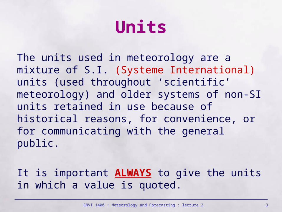
Units
The units used in meteorology are a mixture of S.I. (Systeme International) units (used throughout ‘scientific’ meteorology) and older systems of non-SI units retained in use because of historical reasons, for convenience, or for communicating with the general public.
It is important ALWAYS to give the units in which a value is quoted.
ENVI 1400 : Meteorology and Forecasting : lecture 2 4
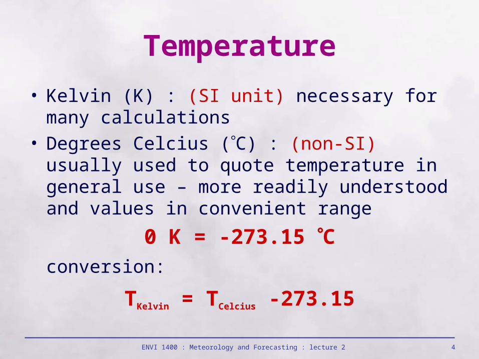
• Kelvin (K) : (SI unit) necessary for many calculations
• Degrees Celcius (C) : (non-SI) usually used to quote temperature in general use – more readily understood and values in convenient range
0 K = -273.15 Cconversion:
TKelvin = TCelcius -273.15
Temperature
ENVI 1400 : Meteorology and Forecasting : lecture 2 5
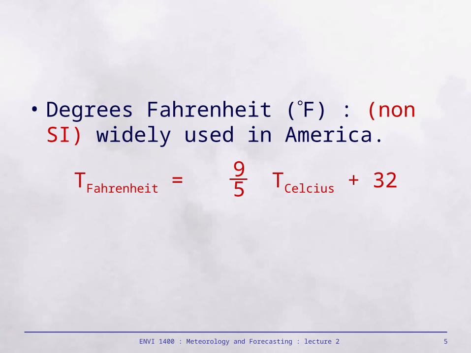
• Degrees Fahrenheit (F) : (non SI) widely used in America.
TFahrenheit = TCelcius + 3295
ENVI 1400 : Meteorology and Forecasting : lecture 2 6
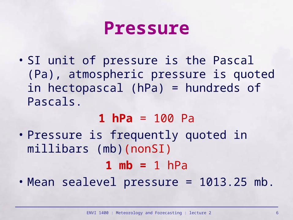
Pressure
• SI unit of pressure is the Pascal (Pa), atmospheric pressure is quoted in hectopascal (hPa) = hundreds of Pascals.
1 hPa = 100 Pa
• Pressure is frequently quoted in millibars (mb)(non SI)
1 mb = 1 hPa
• Mean sea level pressure = 1013.25 mb.
ENVI 1400 : Meteorology and Forecasting : lecture 2 7
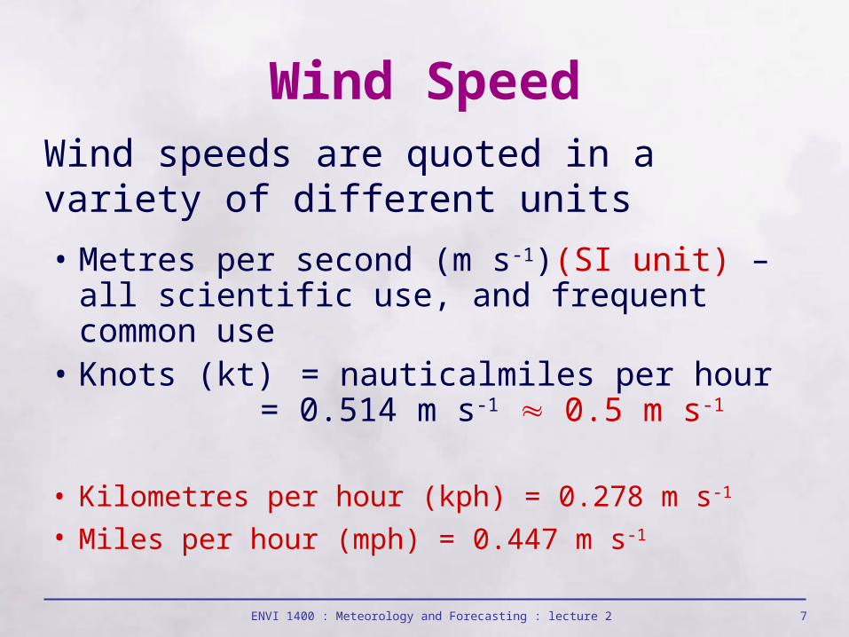
Wind Speed
• Metres per second (m s-1)(SI unit) – all scientific use, and frequent common use
• Knots (kt) = nautical miles per hour = 0.514 m s-1 0.5 m s-1
• Kilometres per hour (kph) = 0.278 m s-1
• Miles per hour (mph) = 0.447 m s-1
Wind speeds are quoted in a variety of different units
ENVI 1400 : Meteorology and Forecasting : lecture 2 8
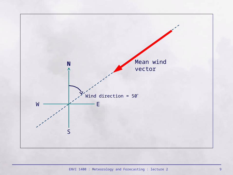
Wind Direction
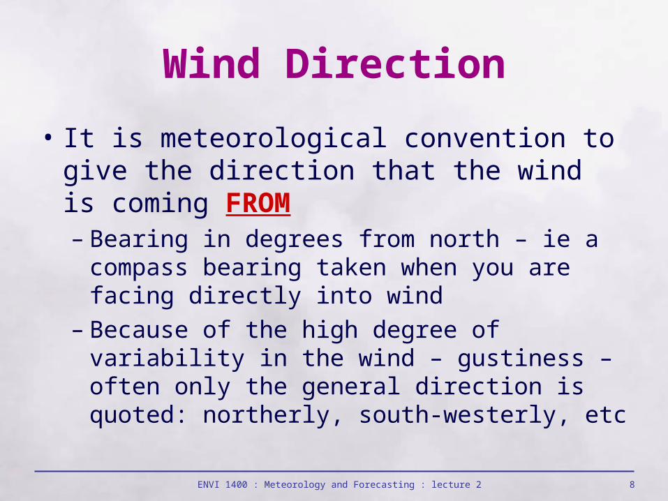
• It is meteorological convention to give the direction that the wind is coming FROM– Bearing in degrees from north – ie a compass
bearing taken when you are facing directly into wind
– Because of the high degree of variability in the wind – gustiness – often only the general direction is quoted: northerly, south-westerly, etc
ENVI 1400 : Meteorology and Forecasting : lecture 2 9
N
S
EW
Mean wind vector
Wind direction = 50
ENVI 1400 : Meteorology and Forecasting : lecture 2 10
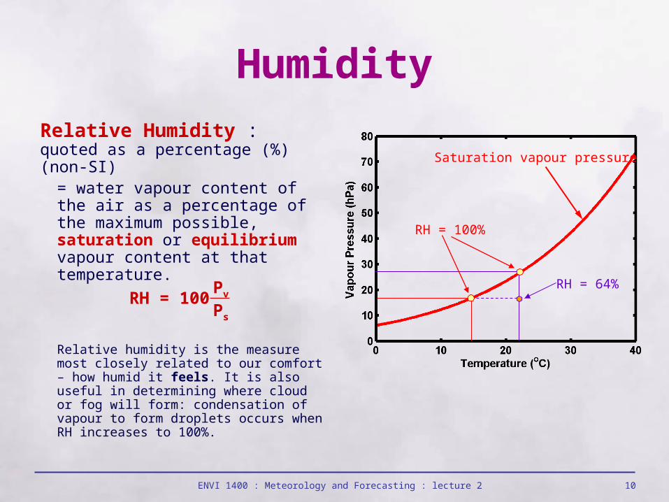
Relative Humidity : quoted as a percentage (%) (non-SI)
= water vapour content of the air as a percentage of the maximum possible, saturation or equilibrium vapour content at that temperature.
Relative humidity is the measure most closely related to our comfort – how humid it feels. It is also useful in determining where cloud or fog will form: condensation of vapour to form droplets occurs when RH increases to 100%.
Humidity
Pv
Ps
RH = 100RH = 64%
RH = 100%
Saturation vapour pressure
ENVI 1400 : Meteorology and Forecasting : lecture 2 11
Dew PointThe temperature to which a parcel of air with constant water vapour content must be cooled, at constant pressure, in order to become saturated.
Dew Point DepressionThe difference between the temperature of a parcel of air, and its dew point temperature.
ENVI 1400 : Meteorology and Forecasting : lecture 2 12
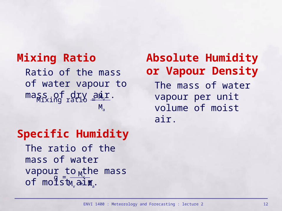
Mixing RatioRatio of the mass of water vapour to mass of dry air.
Specific HumidityThe ratio of the mass of water vapour to the mass of moist air.
Absolute Humidity or Vapour Density
The mass of water vapour per unit volume of moist air.
q = Mv
Mv + Ma
Mixing ratio = Mv
Ma
ENVI 1400 : Meteorology and Forecasting : lecture 2 13
Time• Time is usually quoted in 24-hour form and
in UTC (coordinated universal time). This is (almost) the same as GMT
e.g. 1800 UTC
– Analysis of meteorological conditions to make a forecast requires measurements made at the same time over a very wide area - including multiple time zones (possibly the whole world). Using UTC simplifies the process of keeping track of when each measurement was made
ENVI 1400 : Meteorology and Forecasting : lecture 2 14
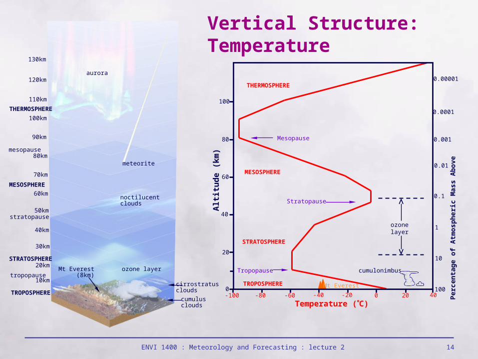
TROPOSPHEREcumulusclouds
cirrostratusclouds
10km
20km
30km
40km
50km
70km
80km
90km
60km
110km
120km
130km
100km
MESOSPHERE
STRATOSPHERE
THERMOSPHERE
Mt Everest(8km)
ozone layer
meteorite
aurora
noctilucentclouds
tropopause
stratopause
mesopause
20
60
40
100
80
0-100 -80 -60 -40 -20 0 4020
100
10
1
0.1
0.01
0.001
0.0001
0.00001
TROPOSPHERE
MESOSPHERE
THERMOSPHERE
STRATOSPHERE
Alt
itu
de
(k
m)
Per
cen
tag
e o
f A
tmo
sph
eric
Mas
s A
bo
ve
Temperature (C)
Tropopause
Stratopause
Mesopause
ozonelayer
Mt Everest
cumulonimbus
Vertical Structure:Temperature
ENVI 1400 : Meteorology and Forecasting : lecture 2 15
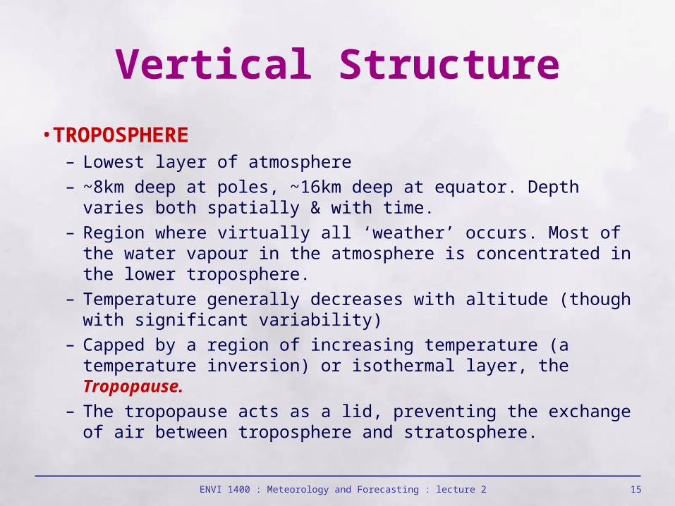
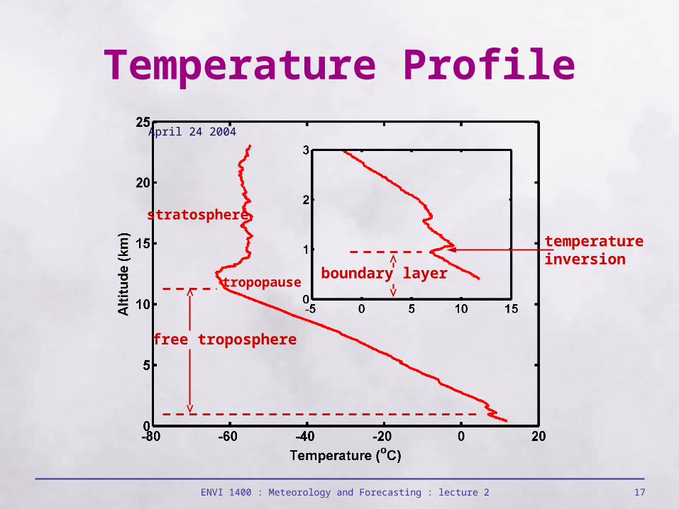
Vertical Structure
• TROPOSPHERE– Lowest layer of atmosphere– ~8km deep at poles, ~16km deep at equator. Depth varies both
spatially & with time.– Region where virtually all ‘weather’ occurs. Most of the water
vapour in the atmosphere is concentrated in the lower troposphere.
– Temperature generally decreases with altitude (though with significant variability)
– Capped by a region of increasing temperature (a temperature inversion) or isothermal layer, the Tropopause.
– The tropopause acts as a lid, preventing the exchange of air between troposphere and stratosphere.
ENVI 1400 : Meteorology and Forecasting : lecture 2 16
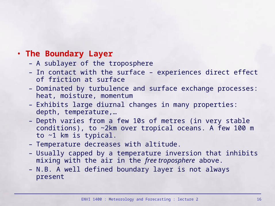
• The Boundary Layer– A sub layer of the troposphere– In contact with the surface – experiences direct effect of friction
at surface– Dominated by turbulence and surface exchange processes:
heat, moisture, momentum– Exhibits large diurnal changes in many properties: depth,
temperature,…– Depth varies from a few 10s of metres (in very stable
conditions), to ~2km over tropical oceans. A few 100 m to ~1 km is typical.
– Temperature decreases with altitude.– Usually capped by a temperature inversion that inhibits mixing
with the air in the free troposphere above.– N.B. A well defined boundary layer is not always present
ENVI 1400 : Meteorology and Forecasting : lecture 2 17
Temperature Profile
tropopause
free troposphere
boundary layer
temperatureinversion
stratosphere
April 24 2004
ENVI 1400 : Meteorology and Forecasting : lecture 2 18
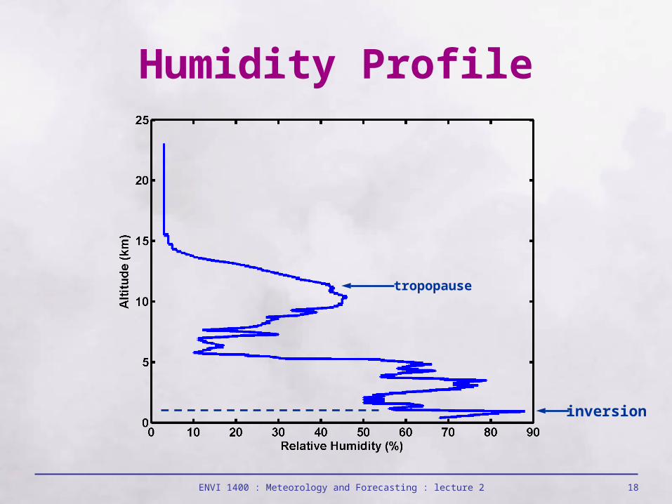
Humidity Profile
tropopause
inversion
ENVI 1400 : Meteorology and Forecasting : lecture 2 19
• STRATOSPHERE– Extends from top of tropsphere to ~50 km.– Temperature generally increases with altitude during summer –
lowest temperature at the equatorial tropopause. Has a more complex structure in winter.
– Contains the majority of atmospheric ozone (O3). Absorption of ultraviolet produce a maximum temperature at the stratopause (sometimes exceeding 0°C).
– Interaction with the troposphere is limited, and poorly understood.
ENVI 1400 : Meteorology and Forecasting : lecture 2 20
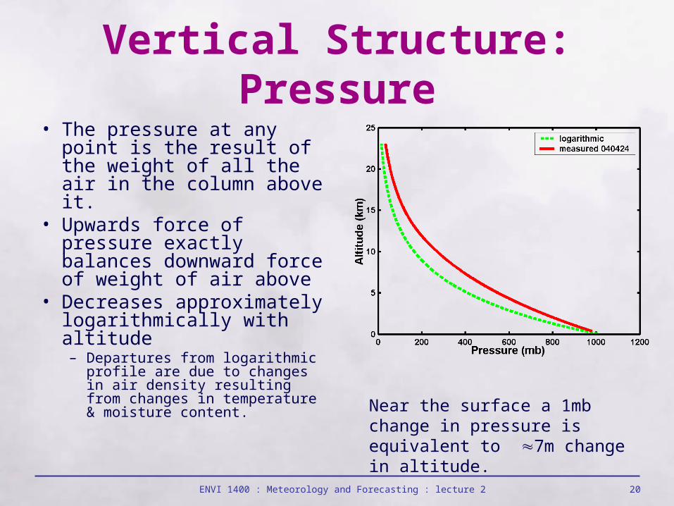
Vertical Structure: Pressure
• The pressure at any point is the result of the weight of all the air in the column above it.
• Upwards force of pressure exactly balances downward force of weight of air above
• Decreases approximately logarithmically with altitude– Departures from logarithmic
profile are due to changes in air density resulting from changes in temperature & moisture content.
Near the surface a 1mb change in pressure is equivalent to 7m change in altitude.
ENVI 1400 : Meteorology and Forecasting : lecture 2 21
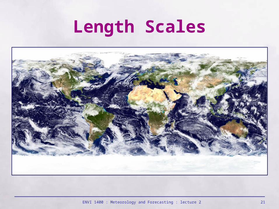
Length Scales
ENVI 1400 : Meteorology and Forecasting : lecture 2 22
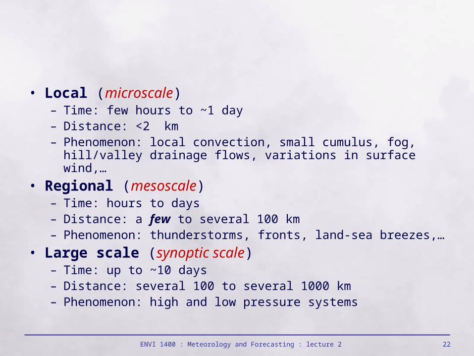
• Local (microscale)– Time: few hours to ~1 day– Distance: <2 km– Phenomenon: local convection, small cumulus, fog, hill/valley
drainage flows, variations in surface wind,…
• Regional (mesoscale)– Time: hours to days– Distance: a few to several 100 km– Phenomenon: thunderstorms, fronts, land-sea breezes,…
• Large scale (synoptic scale)– Time: up to ~10 days– Distance: several 100 to several 1000 km– Phenomenon: high and low pressure systems
ENVI 1400 : Meteorology and Forecasting : lecture 2 23
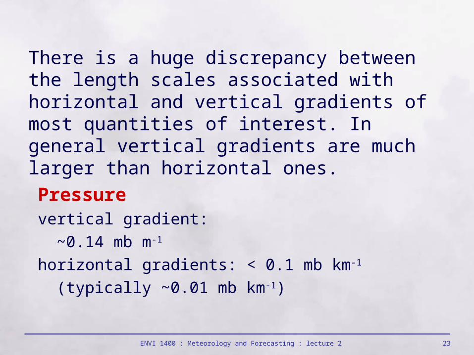
There is a huge discrepancy between the length scales associated with horizontal and vertical gradients of most quantities of interest. In general vertical gradients are much larger than horizontal ones.
Pressurevertical gradient:
~0.14 mb m-1
horizontal gradients: < 0.1 mb km-1
(typically ~0.01 mb km-1)
ENVI 1400 : Meteorology and Forecasting : lecture 2 24
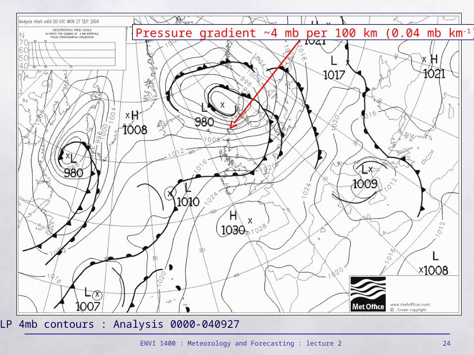
Pressure gradient ~4 mb per 100 km (0.04 mb km-1)
SLP 4mb contours : Analysis 0000-040927
ENVI 1400 : Meteorology and Forecasting : lecture 2 25
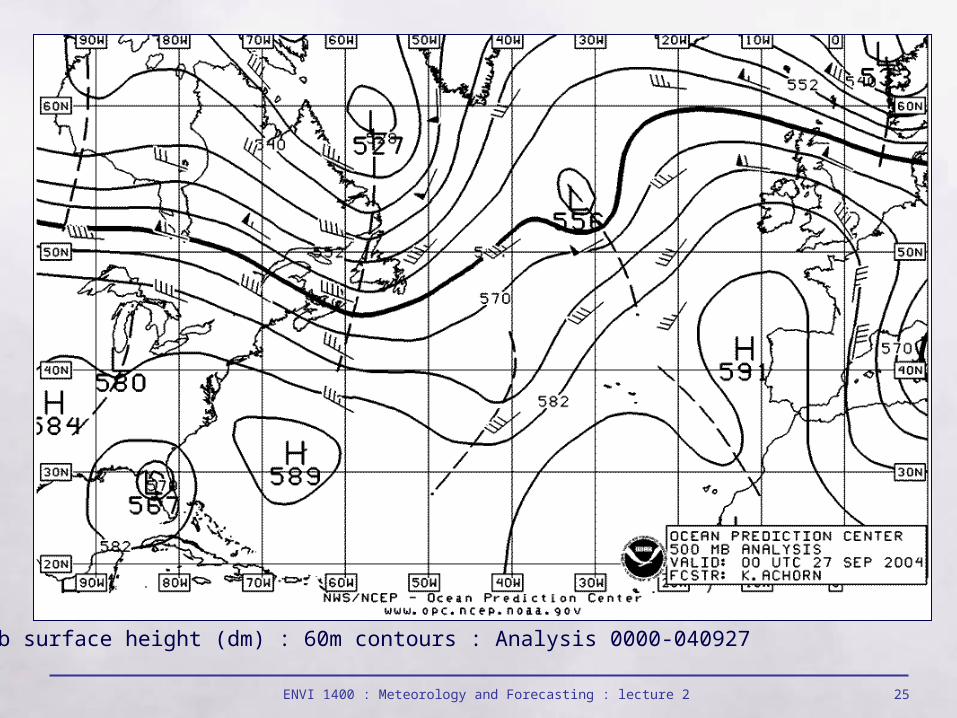
500mb surface height (dm) : 60m contours : Analysis 0000-040927
ENVI 1400 : Meteorology and Forecasting : lecture 2 26
Temperaturevertical gradients:
typically ~0.01 °C m-1
can be larger locally, e.g. boundary layer temperature inversion up to ~0.2 °C m-1
horizontal gradients:
On a large scale typically < 1°C per 100 km (0.01 °C km-1), up to ~5 °C per 100 km within frontal zones. Local effects (e.g. solar heating in sheltered spots) may result in larger gradients on small scales.
N.B. How warm we feel is not a good indicator of the air temperature.
ENVI 1400 : Meteorology and Forecasting : lecture 2 27
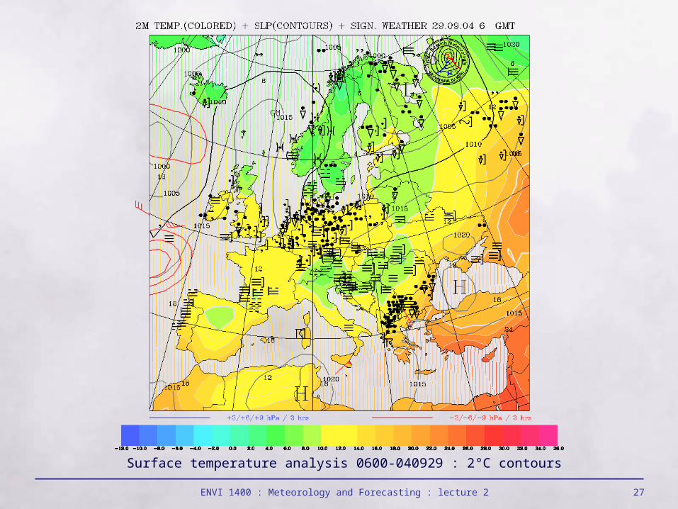
Surface temperature analysis 0600-040929 : 2°C contours
ENVI 1400 : Meteorology and Forecasting : lecture 2 28
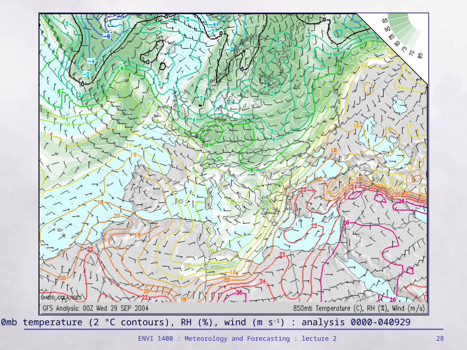
850mb temperature (2 °C contours), RH (%), wind (m s-1) : analysis 0000-040929
ENVI 1400 : Meteorology and Forecasting : lecture 2 29
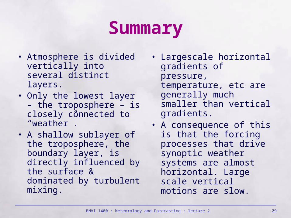
Summary
• Atmosphere is divided vertically into several distinct layers.
• Only the lowest layer – the troposphere – is closely connected to “weather”.
• A shallow sub layer of the troposphere, the boundary layer, is directly influenced by the surface & dominated by turbulent mixing.
• Large scale horizontal gradients of pressure, temperature, etc are generally much smaller than vertical gradients.
• A consequence of this is that the forcing processes that drive synoptic weather systems are almost horizontal. Large scale vertical motions are slow.