
Definition of Image Understanding - uni-hamburg.deneumann/BV-WS-2007/BV-2-07.pdf · 1 1 Definition...
21
1 1 Definition of Image Understanding Image understanding is the task-oriented reconstruction and interpretation of a scene by means of images "scene": section of the real world stationary (3D) or moving (4D) "image": view of a scene projection, density image (2D) depth image (2 1/2D) image sequence (3D) "reconstruction computer-internal scene description and interpretation": quantitative + qualitative + symbolic "task-oriented": for a purpose, to fulfil a particular task context-dependent, supporting actions of an agent 2 Illustration of Image Understanding • • road gully cover hole danger scene image sequence image sequence interpretation
Transcript of Definition of Image Understanding - uni-hamburg.deneumann/BV-WS-2007/BV-2-07.pdf · 1 1 Definition...

1
1
Definition of Image Understanding
Image understanding is the task-oriented reconstruction andinterpretation of a scene by means of images
Image understanding is the task-oriented reconstruction andinterpretation of a scene by means of images
"scene": section of the real worldstationary (3D) or moving (4D)
"image": view of a sceneprojection, density image (2D)depth image (2 1/2D)image sequence (3D)
"reconstruction computer-internal scene descriptionand interpretation": quantitative + qualitative + symbolic
"task-oriented": for a purpose, to fulfil a particular taskcontext-dependent, supporting actions of an agent
2
Illustration of Image Understanding
• •
road
gully
coverhole
danger
scene
imagesequence image sequence
interpretation

2
3
Image Understanding as aKnowledge-based Process
object configurations,situations, occurrences
objects, trajectories
scene elements:volumes, 3D-surfaces,
3D-contours
image elements:regions, edges, texture,
optical flow
raw images
high-level vision,scene understanding
objectrecognition
low-level vision,early vision
segmentation,image preprocessing
common senseknowledge
situation models,occurrence models
object models
projectivegeometry
photometry
physics
basic real-worldproperties
events, episodes
4
Abstraction Levels for the Descriptionof Computer Vision Systems
Knowledge level
What knowledge or information enters a process? What knowledge orinformation is obtained by a process?
What are the laws and constraints which determine the behavior of a process?
Algorithmic level
How is the relevant information represented?
What algorithms are used to process the information?
Implementation level
What programming language is used?
What computer hardware is used?

3
5
Example for Knowledge-level Analysis
What knowledge or information enters a process? What knowledge orinformation is obtained by a process?
What are the laws and constraints which determine the behavior of a process?
Consider shape-from-shading:
In order to obtain the 3D shape of an object, it is necessary to- state what knowledge is available (greyvalues, surface
properties, illumination direction, etc.)- state what information is desired (e.g. qualitative vs.
quantitative)- exploit knowledge about the physics of image formation
6
"natural images"
Image Formation
Images can be generated by various processes:- illumination of surfaces, measurement of reflections
- illumination of translucent material, measurement of irradiation
- measurement of heat (infrared) radiation
- X-ray of material, computation of density map
- measurement of any features by means of a sensory array
physical signal
sensory array

4
7
Formation of Natural Images
Intensity (brightness) of a pixel depends on
1. illumination (spectral energy, secondary illumination)
2. object surface properties (reflectivity)
3. sensor properties
4. geometry of light-source, object and sensor constellation (angles, distances)
5. transparency of irradiated medium (mistiness, dustiness)
8
Qualitative Surface PropertiesWhen light hits a surface, it may be• absorbed• reflected• scattered
Simplifying assumptions:• Radiance leaving at a point is due to radiance arriving at this point• All light leaving the surface at a wavelength is due to light arriving
at the same wavelength• Surface does not generate light internally
in general, all effects may be mixed
The "amount" of reflected light may depend on:• the "amount" of incoming light• the angles of the incoming light w.r.t. to the surface orientation• the angles of the outgoing light w.r.t. to the surface orientation

5
9
Photometric Surface Propertiessurfacenormal
viewingdirection
illuminationdirection
θiθv
x
y
φiφv
θi, θv polar (zenith) angles
φi, φv azimuth angles
In general, the ability of a surface to reflect light is given by theBi-directional Reflectance Distribution Function (BRDF) r:
δE = irradiance of light sourcereceived by the surface patchδL = radiance of surface patchtowards viewer
For many materials the reflectance properties are rotation invariant,in this case the BRDF depends on θi, θv, φ, where φ = φi - φv.
δL(θv, φv)r(θi, φi; θv, φv) = δE(θi, φi)
10
Intensity of Sensor Signalslight source
surface
sensor
Intensities of sensor signals depend on- location x, y on sensor plane- instance of time t- frequency of incoming light wave λ- spectral sensitivity of sensor
x
y
light distribution forsensor
sensitivity function of sensorspectral energy distribution
f(x,y, t) = C(x,y, t,λ)S(λ )dλ∫
0
∞

6
11
Multispectral Images
Sensors with separate channels of different spectral sensitivitiesgenerate multispectral images:
f1( x, y,t) = C(x,y, t,λ )S1(λ)dλ0
∞
∫
f2(x,y, t ) = C(x,y,t,λ )S2(λ )dλ0
∞
∫
f3(x,y, t ) = C(x,y,t,λ )S3(λ )dλ0
∞
∫
Example:R (red) 650 nm center frequency
G (green) 530 nm center frequency
B (blue) 410 nm center frequency
S(λ)
λ
λ
λ
12
Spectral Sensitivity of Human Eyes
Standardized wavelengths:red = 700 nm, green = 546.1 nm, blue = 435.8 nm

7
13
Non-unique Sensor Response
Different spectral distributions may lead to identical sensorresponses and hence cannot be distinguished
�
f(x, y, t) = C1(x, y, t,λ )S(λ )dλ0
∞
∫ = C2(x, y, t,λ )S(λ )dλ0
∞
∫
different spectral energy distributions
Example:
S(λ) S(λ)
λ λ
C1(λ)
C2(λ)
14
Dimensions of Colour
Human perception of colour distinguishes between 3 dimensions:- hue- saturation- brightness
yellowgreen
blueviolet
red
orange
hue
saturation
colour circle
brightness
saturation
y
r
gb
white
black
NCS* colour spindle
* Swedish Natural Colour System
chromaticity

8
15
RGB Images of a Natural Scene
R+G+B R G B
Here, single colour images are rendered as greyvalue intensity images:stronger spectral intensity = more brightness
16
Primary and Secondary ColoursPrimary colours:red, green, blue
Secondary colours:magenta = red + bluecyan = green + blueyellow = red + green
aus: Gonzales & WoodsDigital Image ProcessingPrentice Hall 2002
9
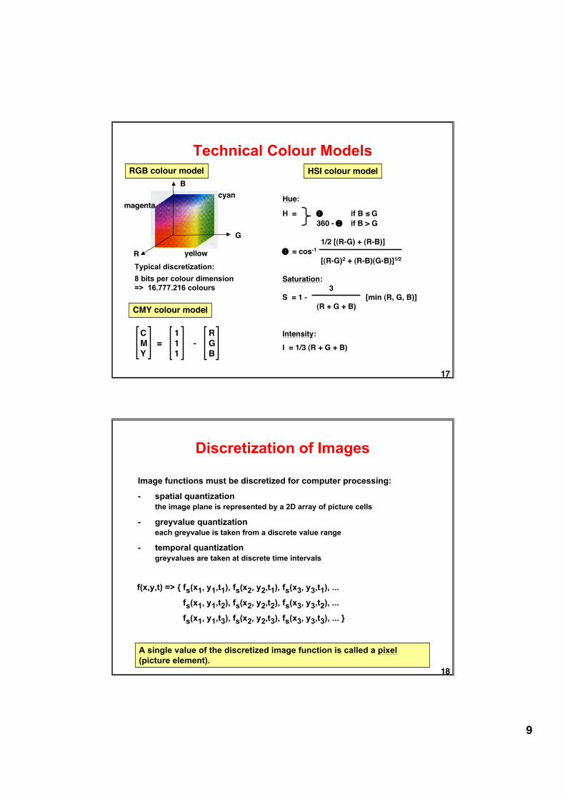
17
Technical Colour ModelsRGB colour model
R
G
B
magentacyan
yellowTypical discretization:8 bits per colour dimension=> 16.777.216 colours
CMY colour model
C 1 RM = 1 - GY 1 B
HSI colour model
Hue:
H = Θ if B ≤ G360 - Θ if B > G
1/2 [(R-G) + (R-B)]Θ = cos-1
[(R-G)2 + (R-B)(G-B)]1/2
Saturation: 3
S = 1 - [min (R, G, B)](R + G + B)
Intensity:I = 1/3 (R + G + B)
18
Discretization of Images
Image functions must be discretized for computer processing:
- spatial quantizationthe image plane is represented by a 2D array of picture cells
- greyvalue quantizationeach greyvalue is taken from a discrete value range
- temporal quantizationgreyvalues are taken at discrete time intervals
f(x,y,t) => { fs(x1, y1,t1), fs(x2, y2,t1), fs(x3, y3,t1), ...
fs(x1, y1,t2), fs(x2, y2,t2), fs(x3, y3,t2), ...
fs(x1, y1,t3), fs(x2, y2,t3), fs(x3, y3,t3), ... }
A single value of the discretized image function is called a pixel(picture element).

10
19
Spatial Quantization
Rectangular grid
Note that samples of ahexagonal grid are equallyspaced along rows, withsuccessive rows shifted byhalf a sampling interval.
Hexagonal grid
Triangular grid
Greyvalues represent thequantized value of thesignal power falling into agrid cell.
• • • • • •• • • • • •
20
Reconstruction from Samples
Under what conditions can the original (continuous) signal bereconstructed from its sampled version?
Consider a 1-dimensional function f(x):
• •• •
•
••
• •• •
• • •
x
f(x)
•
Reconstruction is only possible, if "variability" of function is restricted.

11
21
Sampling Theorem
Shannon´s Sampling Theorem:
A bandlimited function with bandwidth W can be exactlyreconstructed from equally spaced samples, if the samplingdistance is not larger than 1
2W
bandwidth = largest frequency contained in signal(=> Fourier decomposition of a signal)
Analogous theorem holds for 2D signals with limited spatialfrequencies Wx and Wy
22
Aliasing
original 143 x 128 71 x 64 35 x 32
Sampling an image with fewer samples than required by the samplingtheorem may cause "aliasing" (artificial structures).
Example:
To avoid aliasing, bandwidth of image must by reduced prior to sampling.(=> low-pass filtering)

12
23
Reconstructing the Image Functionfrom Samples
Formally, a continuous function f(t) with bandwidth W can be exactlyreconstructed using sampling functions si(t):
si( t) = 2W sin 2πW t − i / (2W)[ ]2πW t − i / (2W)[ ]
i2W
t
si(t)
x(t) = 12W
i=−∞
∞
∑ x ( i2W
) Si(t)
sample values
In practice, image functions are generated from samples by interpolation.
An analogous equation holds for 2D.
24
Sampling TV SignalsPAL standard:
- picture format 3 : 4- 25 full frames (50 half frames) per second- interlaced rows: 1, 3, 5, ... , 2, 4, 6, ...- 625 rows per full frame, 576 visible- 64 µs per row, 52 µs visible- 5 MHz bandwidth
Only 1D sampling is required because of fixed row structure.
Sampling intervals of Δt = 1/(2W) = 10-7s = 100 ns give maximalpossible resolution.
With Δt = 100 ns, a row of duration 52 µs gives rise to 520 samples.In practice, one often chooses 512 pixels per TV row.=> 576 x 512 = 294912 pixels per full frame=> rectangular pixel size with width/height =( ) / ( ) = 1,5
4512
3576
1,51,0

13
25
Sampling of Binary Images (1)
Problem: Shapes may change under digitization
26
Sampling of Binary Images (2)
This cannot be solved by using Shannon´s Theorem since binary images arenot bandlimited.
Problem: Shapes may change under digitization

14
27
Shape Preserving Sampling Theorem:The shape of an r-regular image can be correctly reconstructedafter sampling with any sampling grid, if the grid point distance isnot larger than r.
Shape Preserving Sampling Theorem (1)
Stelldinger, Köthe 2003
"grid point distance": maximal distance from arbitrary sampling point tothe next sampling point
"r-regular binary image":
osculating r-discs at eachboundary point of the shape
⇒ curvature bounded by 1/r⇒ bounded thinness of parts⇒ minimal distance between parts
28
Shape Preserving Sampling Theorem (2)
What does correct reconstruction mean?
Topological and geometric similarity criterion:
One shape can be mapped onto the other by twisting the whole plane,such that the displacement of each point is smaller than r.

15
29
Sampling of Shapes in Arbitrary Images (1)
The previous sampling theorem also holds for greyvalue images, ifeach level set is an r-regular shape.A "level set" is the set where the image is brighter than a giventhreshold value.
sampling + reconstruction
30
Sampling of Shapes in Arbitrary Images (2)
Reconstruction after sampling from r-regular originals
The generalization to higher dimensions has been recently solved.

16
31
Comparison of the Sampling Theorems
same shape as theoriginal image
identical tooriginal image
reconstructedimage
regularization:unsolved problem
band-limitation:efficient algorithms
(but shapes may change!)
prefiltering
arbitrary gridsrectangular grid2D samplinggrid
2D(partly generalizable to n-D)
1D(generalizable to n-D)
dimension ofdefinition
equation
r-regularbandlimited withbandwidth W
necessaryimage property
Shape PreservingSampling Theorem
Shannon´sSampling Theorem
Wdr
21
2´ <⎟
⎠⎞⎜
⎝⎛ = rr <´
32
Quantization of Greyvalues
Quantization of greyvalues transforms continuous values of asampled image function into digital quantities.
Typically 2 ... 210 quantization levels are used, depending on task.
Less than 29 quantization levels may cause artificial contours forhuman perception.
Example:
256 16 8 4 2

17
33
Uniform Quantization
zmax0
q0
qN-1Equally spaced discrete valuesq0 ... qN-1 represent equal-widthgreyvalue intervals of thecontinuous signal.
Typically N = 2K for K = 1 ... 10
Uniform quantization may "waste" quantization levels, if greyvaluesare not equally distributed.
34
Nonlinear Quantization Curves
E.g. fine resolution for "interesting" greyvalue ranges, coarseresolution for less interesting greyvalue ranges.
z
qExample:Low greyvalues are mappedinto more quantization levelsthan high greyvalues.
Note:Subjective brightness in human perception depends (roughly)logarithmically on the actual (measurable) brightness.To let the computer see brightness as humans, use a logarithmicquantization curve.

18
35
Optimal Quantization (1)
Assumption:Probability density p(z) for continuous greyvalues and number ofquantization levels N are known.
Goal:Minimize mean quadratic quantization error dq by choosing optimalinterval boundaries zn and optimal discrete representatives qn.
dq2 = (z − qn)2
zn
zn+1
∫n=0
N−1∑ p(z)dz
δδzn
dq2 = (zn − qn−1)
2p(zn) − (zn − qn)2p(zn) = 0 for n = 1 ... N-1
δδqn
dq2 = −2 (z − qn
zn
zn+1
∫ )p(z)dz = 0 for n = 0 . .. N - 1
Minimizing by setting the derivatives zero:
36
Optimal Quantization (2)Solution for optimal quantization:
zn =12
(qn−1+ qn) for n= 1 .. . N- 1 when p(zn) > 0
qn =
zp(z)dzzn
zn+1
∫
p(z)dzzn
zn+1
∫ for n = 0 ... N - 1
Each interval boundary must be in the middle of the corresponding quantizationlevels.
Each quantization level is the center-of-gravity coordinate of the correspondingprobability density area.
p(z)
0 zmaxz1 z2 z3
q0 q1 q2
Optimal quantizationcan be determined byan iterative algorithmbeginning with anarbitrary choice of z1

19
37
Binarization
For many applications it is convenient to distinguish only between 2greyvalues, "black" and "white", or "1" and "0".
Example: Separate object from background
Binarization = transforming an image function into a binary image
g(x, y) =>
Thresholding:
0 if g(x, y) < T
1 if g(x, y) ≥ TT is threshold
Thresholding is often applied to digital images in order to isolateparts of the image, e.g. edge areas.
38
Threshold Selection by Trial and Error
A threshold which perfectly isolates an image component must notalways exist.
Selection by trial and error:
Select threshold until some image property is fulfilled, e.g.
line strength ⇒ d0
number of connected components ⇒ n0
Number of trials may be small if logarithmic search can be used.
Example:
At most 8 trials are needed to select a threshold 0 ≤ T ≤ 255 whichbest approximates a given q0.
q =
# white pixels# black pixels
⇒ q0

20
39
Distribution-based Threshold Selection
The greyvalue distribution of the image function may show a bimodality:
p(z)
zplausible choice of threshold
Two methods for finding a plausible threshold:
1. Find "valley" between two "hills"
2. Fit hill templates and compute intersection
h(z)
z
Typically, computations are based onhistograms which provide a discreteapproximation of a distribution.
p(z)
z
40
Threshold Selection Based onReference Positions
In many applicatons, the approximate position of image componentsis known a priori. These positions may provide useful referencegreyvalues.
Example: a
bT =
a + b2
possible choiceof threshold:
Threshold selection and binarization may be decisively facilitated bya good choice of illumination and image capturing techniques.

21
41
Image Capturing for Thresholding
If the image capturing process can be controlled, thresholding can befacilitated by a suitable choice of• illumination• camera position• object placement• background greyvalue or colour• preprocessing
Example: BacklightingIllumination from the rear gives bright background and shadowed object
Example: Slit illuminationOn a conveyor belt illuminated bya light slit at an angle, elevationsgive rise to displacements whichcan be recognized by a camera.
empty object present


![Understanding Deep Image Representations by Inverting Them · Most image understanding and computer vision methods build on image representations such as textons [17], his-togram](https://static.fdocuments.net/doc/165x107/5ed200a23dafc82aeb3aa2fe/understanding-deep-image-representations-by-inverting-them-most-image-understanding.jpg)


