NBER WORKING PAPER SERIES

DEFINING CLUSTERS OF RELATED INDUSTRIES

Mercedes DelgadoMichael E. Porter

Scott Stern

Working Paper 20375http://www.nber.org/papers/w20375

NATIONAL BUREAU OF ECONOMIC RESEARCH1050 Massachusetts Avenue

Cambridge, MA 02138August 2014

This project has been funded by a grant from the Economic Development Administration of the U.S.Department of Commerce. We received financial support from Harvard Business School. We thankBill Simpson, Xiang Ao, Rich Bryden, and Sam Zyontz for their invaluable assistance with the analysis.We also acknowledge the insightful comments of two anonymous reviewers, Harald Bathelt, Ed Feser,Frank Neffke, Juan Alcacer, Bill Kerr, Fiona Murray, Christian Ketels, James Delaney, Brandon Stewart,Muhammed Yildirim, Ram Mudambi, Sergiy Protsiv, Jorge Guzman, Sarah Jane Maxted and the participantsin the Industry Studies Association Conference, NBER Productivity Seminar, Temple University Seminar,and the Symposium on the Use of Innovative Datasets for Regional Economic Research at GeorgeWashington University. The views expressed herein are those of the authors and do not necessarilyreflect the views of the National Bureau of Economic Research.

At least one co-author has disclosed a financial relationship of potential relevance for this research.Further information is available online at http://www.nber.org/papers/w20375.ack

NBER working papers are circulated for discussion and comment purposes. They have not been peer-reviewed or been subject to the review by the NBER Board of Directors that accompanies officialNBER publications.

© 2014 by Mercedes Delgado, Michael E. Porter, and Scott Stern. All rights reserved. Short sectionsof text, not to exceed two paragraphs, may be quoted without explicit permission provided that fullcredit, including © notice, is given to the source.

Defining Clusters of Related IndustriesMercedes Delgado, Michael E. Porter, and Scott SternNBER Working Paper No. 20375August 2014JEL No. R0,R1

ABSTRACT

Clusters are geographic concentrations of industries related by knowledge, skills, inputs, demand,and/or other linkages. A growing body of empirical literature has shown the positive impact of clusterson regional and industry performance, including job creation, patenting, and new business formation.There is an increasing need for cluster-based data to support research, facilitate comparisons of clustersacross regions, and support policymakers and practitioners in defining regional strategies. This paperdevelops a novel clustering algorithm that systematically generates and assesses sets of cluster definitions(i.e., groups of closely related industries). We implement the algorithm using 2009 data for U.S. industries(6-digit NAICS), and propose a new set of benchmark cluster definitions that incorporates measuresof inter-industry linkages based on co-location patterns, input-output links, and similarities in laboroccupations. We also illustrate the algorithm’s ability to compare alternative sets of cluster definitionsby evaluating our new set against existing sets in the literature. We find that our proposed set outperformsother methods in capturing a wide range of inter-industry linkages, including grouping industries withinthe same 3-digit NAICS.

Mercedes DelgadoTemple University and ISCFox School of BusinessAlter Hall 5421801 Liacouras WalkPhiladelphia, PA 19122mdelgado@temple.edu

Michael E. PorterHarvard UniversityInstitute for Strategy and CompetitivenessLudcke HouseHarvard Business SchoolSoldiers Field RoadBoston, MA 02163mporter@hbs.edu

Scott SternMIT Sloan School of Management100 Main Street, E62-476Cambridge, MA 02142and NBERsstern@mit.edu

2

1. Introduction

There is an increasing need for useful data tools to measure the cluster composition of

regions, and support regional policy development as well as business strategy. The goal of this

paper is to address this need by providing a rigorous methodology for generating and assessing

sets of cluster definitions – groups of industries closely related by skill, technology, supply,

demand, and/or other linkages. Our approach is novel by comparing the quality of alternative

sets of cluster definitions and also by capturing multiple types of inter-industry linkages. We

implement this clustering algorithm to create a new set of U.S. Benchmark Cluster Definitions

(BCD), capturing a broad range of inter-industry linkages.

Clusters are geographic concentrations of related industries and associated institutions.

The agglomeration of related economic activity is a central feature of economic geography

(Marshall, 1920; Porter, 1990; Krugman, 1991; Ellison and Glaeser, 1997). Marshall (1920)

highlighted three distinct drivers of agglomeration: input-output linkages, labor market pooling,

and knowledge spillovers, which are associated with cost or productivity advantages to firms.

Over time, an extensive literature has broadened the set of agglomeration drivers, including local

demand conditions, specialized institutions, the organizational structure of regional business, and

social networks (Porter, 1990, 1998; Saxenian, 1994; Storper, 1995; Markusen, 1996; Sorenson

and Audia, 2000; among others). Thus, clusters contain a mix of industries related by various

linkages (knowledge, skills, inputs, demand, and others) and supportive institutions.

The bulk of the cluster literature has been based on detailed case studies (Marshall, 1920;

Porter, 1990, 1998; Swann, 1992; Saxenian, 1994). Over time, attention has begun to shift to

larger-scale, quantitative studies across regions and industries (Porter, 2003; Feser, 2005). Using

particular cluster definitions, studies have shown that the presence of related economic activity

matters for regional and industry performance, including job creation, patenting, and new

business formation (see among others, Feldman and Audretsch, 1999; Porter, 2003; Feser,

Renski, and Goldstein, 2008; Glaeser and Kerr, 2009; Delgado, Porter, and Stern, 2010, 2014;

Neffke, Henning, and Boschma, 2011).1 This evidence has informed key questions of both

research and policy interest: the size of cluster effects, which mechanisms are most important in

driving agglomeration, and how clusters diversify and grow in a region. Based on different

1 See Rosenthal and Strange (2004) and Cortright (2006) for a review of economies of agglomeration studies.

3

definitions of clusters, covering different portions of the economy ranging from high

technological intensity industries to manufacturing to all industries defined in the industrial

classification system, existing research has generated a range of results on these issues. However,

the lack of a comprehensive methodology, and a way to compare alternative sets of cluster

definitions, makes it difficult to reconcile key findings. This paper addresses this issue by

developing a novel clustering algorithm to generate, assess and compare alternative sets of

cluster definitions.

Cluster definitions are groups of industries related by skill, technology, supply, demand,

and/or other linkages. This paper focuses on regionally comparable cluster definitions (i.e., the

industries that constitute a cluster (e.g., Biopharmaceuticals) are the same for all regions). Inter-

industry linkages are identified through the co-location patterns of industries across regions, or

with a range of national data available across industries. The identified linkages are used to

group industries into a set of defined clusters, allowing clusters to be compared across regions.

To generate a set of cluster definitions, we use clustering analysis – numerical methods

for the classification of similar objects into groups (Everitt et al., 2011; Grimmer and King,

2011). Our algorithm generates many different cluster configurations, Cs, through a clustering

function that utilizes a particular measure of the relatedness between any two industries and well-

specified parameter choices (e.g., the number of groups). Each configuration is composed of

mutually exclusive groups of related industries (i.e., clusters). The algorithm then provides

scores that assess the quality of each C (i.e., its ability to capture meaningful inter-industry

linkages within clusters). This allows us to identify the configuration, C*, that best captures

certain types of inter-industry links. Because an algorithm cannot perfectly substitute for expert

judgment, the methodology concludes with an expert assessment and adjustment of individual

clusters in C* to determine a final set of cluster definitions, C**.

Our paper contributes to the literature on clusters and economies of agglomeration in

several ways. First, the clustering algorithm allows us to compare the quality of alternative sets

of clusters using a common approach that generates objective scores (i.e., most clustering

methods do not provide scores to help compare across groupings (Everitt et al., 2011; Grimmer

and King, 2011)). We can assess cluster configurations that are generated using different inter-

industry linkage measures. For example, we can evaluate Cs generated using pairwise industry

co-location patterns to those based on input-output or other measures. We can also compare

4

existing sets of cluster definitions. The ability to score sets of clusters can help identify the

appropriate sets for addressing particular research and policy questions.

Our scoring approach utilizes a basic clustering principle: creating groupings so that

industries within a cluster are more related to each other than to industries in other clusters based

on various measures of inter-industry linkages. The score for a given C depends on how well it

captures various types of industry linkages. However, what constitutes a useful set of cluster

definitions may change depending on the particular research and policy question. Some studies

may be interested in a particular type of industry link (e.g., labor occupational links), making sets

of cluster definitions that perform better in that link more useful.

Second, our algorithm allows for experimentation with multiple inter-industry linkage

measures used in the economies of agglomeration literature, including input-output linkages,

occupational linkages, the co-location patterns of industries, and combinations among them. We

can then examine the cluster configurations generated based on these different measures. The

methodology can incorporate additional inter-industry linkage measures as they become

available (e.g., a measure that specifically captures knowledge linkages), and score their

resulting cluster sets.

Third, although generating cluster definitions will require expert judgment for some

individual clusters, our algorithm is transparent. In the last stage of the algorithm, there is room

for expert judgment to correct for inevitable anomalies that arise due to data imperfections and

industry definitions. For example, in a given C*, there could be industry outliers that do not seem

to belong to their assigned cluster. These can be reallocated to their “next best” cluster using a

score that assesses the relatedness of the particular industry with another cluster, using a

transparent process. Users can assess how adjustments (re-allocations of industries, combining or

dividing clusters) impact cluster scores.

Another important contribution of this paper is that we implement our method to generate

a new set of benchmark cluster definitions for the U.S. (BCD or C**), which captures a wide

array of inter-industry linkages. The U.S.-based empirical analysis focuses on grouping 778 6-

digit NAICS industries in manufacturing and services in 2009, and uses County Business

Patterns (CBP), the Benchmark Input-Output Account of the United States, and Occupational

Employment Statistics (OES) datasets to define multiple industry relatedness measures.

5

The proposed BCD is generated using inter-industry measures of co-location patterns of

employment and the number of establishments, input-output links, and labor occupation links,

and contains 51 clusters. We examine the relative performance of the BCD and three existing

sets of (mutually exclusive) cluster definitions: industries within the same 3-digit NAICS, Porter

(2003), and Feser (2005). Grouping industries within the same 3-digit NAICS scores poorly in

capturing multiple inter-industry linkages, which is perhaps not surprising since the industrial

classification system groups industries based on the similarities of their products/services, not on

their inter-industry complementarities. Moreover, manufacturing and service industries belong to

different parts of the NAICS, so that products and services are definitionally unrelated.

Numerous empirical studies on economies of agglomeration have relied solely on industry codes

to define inter-industry relatedness, potentially limiting their ability to capture a broad array of

relevant industry linkages.

Our benchmark set scores higher in capturing a broader range of inter-industry linkages

than the three other prominent sets of cluster definitions. The BCD also scores better or the same

as the other sets in input-output linkages and shared labor occupations.

While the analysis is based on U.S. data, our clustering methodology can be implemented

in other large and integrated economies with sufficient data availability. At present, however,

U.S. data offers several advantages. Comparably large and diversified economic areas like the

EU have heterogeneous data accessibility across countries, and current and past barriers to trade

across locations can limit economies of agglomeration. Smaller economies (like the Nordics)

have access to rich data, but their relative small size leads to specialization in a narrow range of

industries.

Our benchmark cluster definitions offer a useful tool for research and policy on regional

economic development. They allow the comparison of clusters across locations and over time by

mapping the defined clusters into regional units and measuring the specialization patterns of

regions in the clusters. Using the BCD, the U.S. Cluster Mapping Project has created a detailed

regional cluster dataset that facilitates comparisons across regions and across clusters on

numerous dimensions.2 For example, the Boston, MA and San Diego, CA Economic Areas have

high employment specialization in Biopharmaceuticals, but the size and breadth of the cluster is

2 The U.S. Cluster Mapping website (http://clustermapping.us/) is supported by the U.S. Economic Development Administration, U.S. Department of Commerce.

6

lower in San Diego, which lacks specialization in biological products (except in-vitro diagnostic

substances). The Project also includes data on the business environment and cluster institutions

to inform research and policy. This data tool can be used in combination with cluster methods

that focus on examining region-specific links among firms, individuals, and supportive

institutions in clusters to shed light on the mechanisms at play in particular regional clusters.

The rest of the paper is organized as follows: Section 2 reviews the literature on industry

cluster definitions. Section 3 describes our clustering algorithm. In Section 4, we discuss our

main findings regarding the generation and assessment of cluster configurations, and Section 5

proposes a set of benchmark cluster definitions. In Section 6 we compare the BCD to existing

sets of cluster definitions in the literature, and discuss some research and policy applications.

Section 7 concludes.

2. Defining Industry Clusters

There are various types of economies of agglomeration identified in the literature,

including input-output linkages, labor market pooling, knowledge spillovers, sophisticated local

demand, specialized institutions, and the organizational structure of business and social networks

(Marshall, 1920; Porter, 1990, 1998; Swann, 1992; Saxenian, 1994; Storper, 1995; Markusen,

1996; among others). These economies of agglomeration manifest themselves in clusters –

geographic concentrations of related industries and associated institutions. Within regional

clusters, firms and associated institutions (i.e., trade organizations, universities, and local

government) can operate more efficiently and innovate faster due to sharing common

technologies, infrastructure, pools of knowledge and skills, inputs, and responding to demanding

local customers.

To implement cluster research and policy, however, we need to measure the boundaries

of clusters: What set of related economic activity and institutions constitutes a cluster? Two main

approaches to defining clusters have developed over the last 20 years: clusters based on inter-

industry linkages inferred from multi-region analysis (which we refer to as comparable cluster

definitions) and cluster definitions based on observed linkages among industries or firms in a

single region (which we refer to as region-specific cluster definitions). Many empirically derived

cluster definitions have been generated by researchers and practitioners over the years based on

both approaches (see Cortright (2006) and Feser et al., (2009) for a review). The goal of this

7

paper is to develop a novel methodology to generate and assess sets of comparable cluster

definitions. We next explain both approaches to define clusters and the contribution of our

clustering method to the literature.

2.1 Comparable Cluster Definitions

A set of comparable cluster definitions allocates individual industries to specific clusters

(e.g., Biopharmaceuticals), allowing clusters to be compared across locations. The defined

clusters are mapped into regional units to measure the cluster specialization of regions. We can

then compare particular clusters across regions, as well as the overall cluster composition of

regions. Regional cluster strength reflects specialization in an array of related industries, not

specialization in a narrowly defined single industry (Porter, 1998, 2003; Feldman and Audretsch,

1999; Delgado et al., 2014). Thus, regional cluster strength is conceptually similar to the notion

of “related variety” introduced by Frenken et al. (2007). For example, a regional cluster with a

high breadth of industries will capture related variety.

There are two types of inter-industry relatedness measures that have been developed in

the literature (see Section 3.1 for a detailed explanation). Some studies use national-level data to

capture particular inter-industry linkages, including knowledge links based on co-patenting (see

e.g., Scherer, 1982; Koo, 2005a; Glaeser and Kerr, 2009); input and output links (see e.g., Feser

and Bergman, 2000; Feser, 2005); skill links (see e.g., Koo, 2005b; Glaeser and Kerr, 2009;

Neffke and Henning, 2013); and product similarity as defined by the industry classification

system (e.g., same 3-digit NAICS). Still other studies define measures based on the co-location

patterns of industries across many regions to capture various types of linkages (Ellison and

Glaeser, 1997; Porter, 2003; Ellison et al., 2010). Only a few studies use the inter-industry

relatedness measures to then define clusters of related industries. We next discuss the main

existing sets of cluster definitions.

Knowledge Clusters. Studies of knowledge clusters focus on a selected set of U.S.

manufacturing industries with high technological intensity. For example, Feldman and Audretsch

(1999) group industries that have a common science and technological base, using the Yale

Survey of R&D Managers. This survey assesses the relevance of key academic disciplines for a

product category. Industries with similar rankings of the importance of different academic

disciplines are grouped into six mutually exclusive clusters. Alternatively, Koo (2005b) groups

8

manufacturing industries into seven mutually exclusive knowledge-based clusters using principal

component factor analysis on an inter-industry patent-citation flow matrix.

Input-Output Clusters. Feser and Bergman (2000) define a set of U.S. manufacturing

clusters using input-output links based on the Benchmark Input-Output Accounts of the United

States. They group input-output classification codes (IO codes) into 23 clusters using principal

component factor analysis on an inter-industry input-output link matrix. The factor analysis

method tends to create highly uneven clusters, with a large number of IO codes grouped into a

few clusters. To address this issue, Feser (2005) develops a new methodology based on

hierarchical clustering on an input-output link matrix for manufacturing and service activities.

This transparent method creates a set of 45 mutually exclusive clusters. Overlapping clusters are

then created in a second stage by identifying secondary IO codes highly related to the primary

codes within a cluster. For each cluster, the method provides scores of the fit of each IO code

within its cluster. The IO codes are then matched to 2002 NAICS codes to create a final set of

clusters of related industries.

Co-Location-Based Clusters. Porter (2003) examines the co-location patterns of narrowly

defined industries in both service and manufacturing to define clusters, following the principle

that co-location reveals the presence of linkages across industries. The methodology first

distinguishes traded and local industries. Local industries are those that serve primarily the local

markets (e.g., retail), whose employment is evenly distributed across regions in proportion to

regional population. Traded industries are those that are more geographically concentrated and

produce goods and services that are sold across regions and countries. The set of traded

industries excludes natural-resource-based industries, whose location is tied to local resource

availability (e.g., mining).

To measure the relatedness between a pair of traded industries (4-digit SIC), Porter

(2003) computes the pairwise correlation of industry employment across states using 1996 data.

This measure of co-location patterns is referred to as the “locational correlation” of employment

(LC-Employment) and could capture various types of inter-industry linkages. Porter (2003) uses

an iterative approach to define clusters rather than a clustering function approach. A set of 41

narrow (mutually exclusive) clusters are created using an iterative process to identify pairs and

then groups of industries highly linked based on statistically significant locational correlations.

In a second stage, a set of broad (overlapping) clusters is created by including other industries

9

that have a high locational correlation with the core industries within the narrow cluster. While

the cluster definitions are mainly based on the empirical patterns of employment co-location

among industries, the Benchmark Input-Output Account of the United States and industry

definitions are used to correct the placement of industries with high co-location but low

economic relatedness. These cluster definitions have proven very useful in the empirical analysis

of the role of clusters on regional performance (see e.g., Porter, 2003; Delgado, Porter, and Stern,

2010, 2014).

2.2 Region-Specific Cluster Definitions

Comparable cluster definitions can capture most economic activities and are necessary

for studies that aim to examine clusters across regions. However, one limitation of any multi-

region cluster approach is that it may overlook specific inter-industry linkages that may exist in

particular regional clusters. These idiosyncratic regional linkages are the focus of the region-

specific cluster definitions. This approach focuses on a single region to measure industry and/or

firm interdependencies and define the region’s clusters. Such studies vary in their industry

coverage, types of economic units (industry, technology classes, or firms), types of regional units

(administrative or non-administrative), and methods.

A small set of papers defines region-specific clusters for a large set of economic

activities. Some of these studies identify specific “driver” industries in which a region has a

competitive advantage. Then they use region-specific inter-industry linkages, such as regional

input-output models, to define the clusters around the driver industries (Hill and Brennan, 2000).

Other studies focus on identifying the (non-administrative) geographic boundaries of a given

cluster. To do so, they examine the spatial density of businesses for particular industries

(Duranton and Overman, 2005) or the spatial density of patents for particular technology classes

(e.g., Kerr and Kominers, 2010; Alcacer and Zhao, 2013). The goal is to identify locations with a

high density of economic activity in a particular field that will facilitate inter-firm connections

and externalities.

The bulk of region-specific cluster definitions are qualitative and based on case studies

that tend to focus on particular clusters (see e.g., Bresnahan and Gambardella (2004); Cortright,

2010; Porter and Ramirez-Vallejo, 2013), for example, the Athletic and Outdoor cluster in

Portland (Cortright, 2010). These studies rely on existing cluster organizations, industry

10

directories, and other primary data collection to identify clusters. They offer rich details on the

firms and institutions within particular defined clusters, but may be less appropriate for

comparing clusters across regions.

The conceptual limitation to region-specific approaches to define clusters is that such

definitions are based on observed linkages among existing economic activities in a region

(Bathelt, Malmberg, and Maskell, 2004; Maskell and Malmberg, 2007; Feser et al., 2009; Bathelt

and Li, 2013). Activities that are not present in a region (e.g., industries, technology classes, and

labor occupations that are not present) are classified as unrelated to the other activities in the

region. However, such non-present activities could be related to the activities in the region, but

historical factors, market imperfections or other factors may have prevented their development.

Region-specific cluster definitions could thus be too narrow (or myopic) in terms of the linkages

captured because they abstract from the linkages that may be present in other locations. Thus,

region-specific cluster definitions could be complemented by comparable cluster definitions

derived from patterns across multiple regions.

This paper creates a new cluster methodology that systematically generates comparable

cluster definitions based on multiple types of inter-industry linkages. This approach provides

scores that assess the ability of each set of definitions to capture high inter-industry linkages

within individual clusters. For example, we can compare the Feser (2005) and Porter (2003) sets

of cluster definitions as well as other sets.

We implement the algorithm and propose a new set of U.S. Benchmark Cluster

Definitions (BCD) that captures a wide variety of inter-industry linkages. This set can be updated

over time as new data (e.g., new industry definitions) becomes available.

3. The Clustering Algorithm

In order to derive clusters of industries, we use cluster analysis, or numerical methods to

classify similar objects (cities, people, genes, industries, etc.) into groups (Everitt et al., 2011). In

contrast to network analysis, where each object is related to any other object,3 cluster analysis

3 For example, some papers focus on defining the “product space” – the network of relatedness between products. Hidalgo et al. (2007) define the product space for exported goods. Other studies focus on specific dimensions of the product space, such as the technology, knowledge, or market space (Jaffe, Trajtenberg, and Henderson, 1993; Neffke et al., 2011; Bloom et al., 2012).

11

creates groups (termed clusters) in such a way that objects in the same cluster are more similar

among themselves than to those in other clusters.

Defining clusters of related industries involves a number of key choices that can be

parameterized in a clustering algorithm. The algorithm includes criteria for scoring alternative

cluster configurations. Once the most promising configuration is identified, the algorithm

addresses outlier industries to develop a final set of cluster definitions.

The clustering algorithm is designed to define mutually exclusive clusters, where each

industry is uniquely assigned to one cluster. The methodology also allows the measurement of

relatedness between any pair of (mutually exclusive) clusters and the creation of overlapping

clusters (with individual industries shared by multiple clusters).

Drawing on Porter (2003), our method first distinguishes between traded industries

(geographically concentrated) and local industries (geographically dispersed). There are 1,088 6-

digit NAICS-2007 industries in the 2009 CBP data (excluding farming and some government

activity). We identify 778 traded industries using the specialization and concentration patterns of

each industry across U.S. regions. In 2009, the traded industries account for 36% of total U.S.

employment, 50.5% of payroll, and more than 90% of patenting activity.4

The analysis focuses on grouping the 778 traded industries in service and manufacturing

into non-overlapping groups. We refer to each cluster configuration as C and its individual

clusters as c. There are five inter-related steps to create and assess each configuration C: (1)

define a similarity matrix Mij that captures the relatedness between any two industries; (2) make

broad parameter choices β; (3) use a clustering function to create a configuration C based on the

similarity matrix and parameter choices (C=F(Mij, β)); (4) calculate performance scores for each

C and identify the most promising configuration C*; and (5) assess and correct the individual

clusters in C* to determine the finalized set of cluster definitions C**. Each of these clustering

algorithm steps is explained in detail below.5

3.1 Step 1: Similarity Matrix

The first step to group related industries into clusters is to define the degree to which each

pair of industries is related. A similarity matrix Mij provides the relatedness between any pair of

4 The complete description of the traded and local categorization can be found on the U.S. Cluster Mapping website. 5 All the steps of the algorithm were implemented using STATA software.

12

industries i and j. The matrix is based on the choice of indicator and the similarity measure.

Indicators used in the literature include employment, number of establishments, measures of

buyer-supplier linkages, and measures of shared labor requirements. The choice of a similarity

measure allows the user to decide how the distance between two industries i and j should be

measured (e.g., correlation coefficient, Euclidean, Jaccard index, or user-defined measures).

There are many alternative similarity matrices. Our analysis focuses on the inter-industry

relatedness measures most frequently used in the field of regional studies to capture economies

of agglomeration. The similarity matrices can be divided into three types. First, there are Mij that

exploit co-location patterns across many regions to capture various types of inter-industry

linkages. This group includes the locational correlation of employment developed by Porter

(2003) and the Ellison and Glaeser (1997) coagglomeration index. Second, there are Mij that

focus on national-level inter-industry linkages, including measures based on national input and

output tables (see Feser and Bergman, 2000; Feser, 2005; Ellison, Glaeser, and Kerr, 2010) and

on labor occupation links (Glaeser and Kerr, 2009). Third, we create multidimensional matrices

that use a combination of these matrices. In what follows, we explain each of these similarity

matrices as well as additional industry linkages we do not directly measure.

Pairwise Industry Co-location Patterns. Before we explain the co-location similarity

matrices used in our analysis, we need to clarify the regional unit used for these measures and the

source of the underlying data. There are two spatial approaches to measure the co-location

patterns of industries across regions: using discrete spatial units like states (Ellison and Glaeser,

1997; Porter, 2003; Ellison, Glaeser, and Kerr, 2010) and using continuous spatial units that are

based on the density of businesses (Duranton and Overman, 2005). Discrete spatial units that

capture relevant regional markets offer a reasonable starting point for understanding co-location

patterns. The differences between discrete and continuous co-location measures in their ability to

capture inter-industry externalities can be tested. For example, Ellison, Glaeser, and Kerr (2010)

show that their co-agglomeration index based on states and an approximation of the continuous

co-agglomeration metric developed by Duranton and Overman (2005) both capture similar inter-

industry Marshallian effects (input-output, skill, and knowledge links). Using continuous spatial

measures is beyond the scope of this paper due to data limitations.

We use meaningful administrative regional units: Economic Areas (EAs) as defined by

the Bureau of Economic Analysis (BEA). EAs represent 179 relevant regional markets that cover

13

the entirety of the continental United States (Johnson and Kort, 2004). The underlying

employment and count of establishments of an EA-industry is sourced from the County Business

Patterns (CBP) 2009 data.6

Locational Correlation (LC). Porter (2003) examines the employment co-location

patterns of pairs of industries to capture inter-industry linkages of various types (e.g.,

technology, skills, supply, or demand links). He defines the locational correlation of employment

(LC-Employment) of a pair of industries as the correlation coefficient between employment in

industry i and employment in industry j in a region r:

(1).

Similarly, we also define an alternative locational correlation based on the count of

establishments in a region-industry:

(2).

Economies of agglomeration channels include firms as well as employees. The presence of

numerous establishments can facilitate inter-firm interactions that result in spillovers (Glaeser

and Kerr, 2009). Thus, the co-location patterns of count of establishments could help capture

inter-industry linkages that are facilitated by the number of businesses.

The correlation coefficient is a well-known distance measure for continuous data used in

clustering analysis (Everitt et al., 2011). The LC measures can be implemented for very granular

industry definitions, and its scale is easy to interpret, with values between -1 and 1. Positive and

large values suggest that there are relevant economic interdependencies between a pair of

industries. For example, if the location of employment (count of establishments) in electronic

computers and software is highly correlated, it would suggest that both industries are linked.

While the LC measures tend to capture relevant linkages, it is possible that in some cases

industries with high co-location may have little economic relatedness but instead capture shared

natural resources. As we discuss further below, this does not limit the usefulness of co-location

measures.

LC also could be sensitive to the size of the regions (Porter, 2003). For example, for pairs

of industries with employment concentrated in large regions (i.e., with many pairs of zero

6 The CBP data is made available at the county, state, and U.S. level. Economic Area data is built up from the county file. CBP data uses cell suppression in certain geography-industries with a small presence of firms. When employment data is suppressed, a range is reported. We utilize the midpoint in the range in our data.

- ( , )ij ir jrLC Employment Correlation Employment Employment

- ( , )ij ir jrLC Establishments Correlation Establishments Establishments

14

activity across regions), the LC could be biased. We limit this problem by using EAs versus

using smaller regional units (like counties) that do not fully capture the regional market. We also

implement several sensitivities to EA size that suggest this problem is limited.7 In our data, the

average LC-Employment and LC-Establishments of a pair of industries are 0.30 and 0.52,

respectively (Table 2).

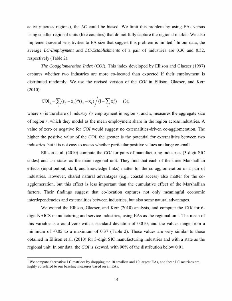
The Coagglomeration Index (COI). This index developed by Ellison and Glaeser (1997)

captures whether two industries are more co-located than expected if their employment is

distributed randomly. We use the revised version of the COI in Ellison, Glaeser, and Kerr

(2010):

(3);

where sri is the share of industry i’s employment in region r; and xr measures the aggregate size

of region r, which they model as the mean employment share in the region across industries. A

value of zero or negative for COI would suggest no externalities-driven co-agglomeration. The

higher the positive value of the COI, the greater is the potential for externalities between two

industries, but it is not easy to assess whether particular positive values are large or small.

Ellison et al. (2010) compute the COI for pairs of manufacturing industries (3-digit SIC

codes) and use states as the main regional unit. They find that each of the three Marshallian

effects (input-output, skill, and knowledge links) matter for the co-agglomeration of a pair of

industries. However, shared natural advantages (e.g., coastal access) also matter for the co-

agglomeration, but this effect is less important than the cumulative effect of the Marshallian

factors. Their findings suggest that co-location captures not only meaningful economic

interdependencies and externalities between industries, but also some natural advantages.

We extend the Ellison, Glaeser, and Kerr (2010) analysis, and compute the COI for 6-

digit NAICS manufacturing and service industries, using EAs as the regional unit. The mean of

this variable is around zero with a standard deviation of 0.010; and the values range from a

minimum of -0.05 to a maximum of 0.37 (Table 2). These values are very similar to those

obtained in Ellison et al. (2010) for 3-digit SIC manufacturing industries and with a state as the

regional unit. In our data, the COI is skewed, with 90% of the distribution below 0.01.

7 We compute alternative LC matrices by dropping the 10 smallest and 10 largest EAs, and these LC matrices are highly correlated to our baseline measures based on all EAs.

2ij ri r rj r r

r rCOI (s x )*(s x ) (1 x )

15

National-Level Inter-Industry Links. We explain the next two similarity matrices that are

based on national-level data: input-output and labor occupation links. Because these measures do

not consider location patterns, they may capture industry interdependencies that are not

geographically bounded.

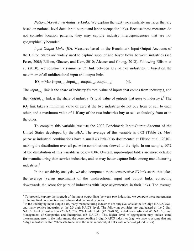
Input-Output Links (IO). Measures based on the Benchmark Input-Output Accounts of

the United States are widely used to capture supplier and buyer flows between industries (see

Feser, 2005; Ellison, Glaeser, and Kerr, 2010; Alcacer and Chung, 2012). Following Ellison et

al. (2010), we construct a symmetric IO link between any pair of industries i,j based on the

maximum of all unidirectional input and output links:

(4).

The i jinput link is the share of industry i’s total value of inputs that comes from industry j, and

the i joutput link is the share of industry i’s total value of outputs that goes to industry j.8 The

IOij link takes a minimum value of zero if the two industries do not buy from or sell to each

other, and a maximum value of 1 if any of the two industries buy or sell exclusively from or to

the other.

To compute this variable, we use the 2002 Benchmark Input-Output Account of the

United States developed by the BEA. The average of this variable is 0.02 (Table 2). Most

pairwise industrial combinations have a small IO link (also documented at Ellison et al., 2010),

making the distribution over all pairwise combinations skewed to the right. In our sample, 90%

of the distribution of this variable is below 0.06. Overall, input-output tables are more detailed

for manufacturing than service industries, and so may better capture links among manufacturing

industries.9

In the sensitivity analysis, we also compute a more conservative IO link score that takes

the average (versus maximum) of the unidirectional input and output links, correcting

downwards the score for pairs of industries with large asymmetries in their links. The average

8 To properly capture the strength of the input-output links between two industries, we compute these percentages excluding final consumption and value-added commodity codes. 9 In the underlying input-output data, many manufacturing industries are only available at the 4/5-digit NAICS level, and many service industries at the 2/3-digit NAICS level. The following activities are aggregated at the 2-digit NAICS level: Construction (23 NAICS), Wholesale trade (42 NAICS), Retail trade (44 and 45 NAICS), and Management of Companies and Enterprises (55 NAICS). This higher level of aggregation may induce some measurement error in the links among the corresponding 6-digit NAICS industries (e.g., we have to assume that any 6-digit industries within Wholesale trade have the same input-output links with other 6-digit industries).

j j jIO Max{input ,input ,output ,output }ij i   i   i   i j

16

and maximum pairwise IO links are highly correlated, and our findings are robust to using these

alternative measures.10

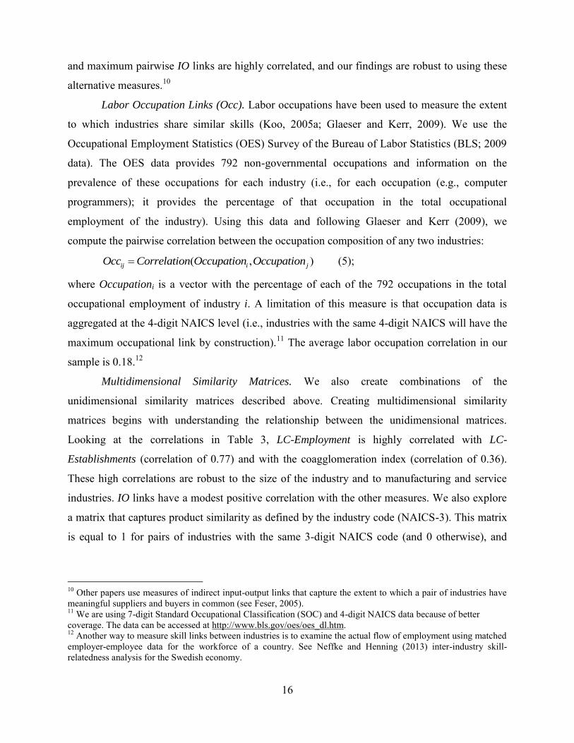
Labor Occupation Links (Occ). Labor occupations have been used to measure the extent

to which industries share similar skills (Koo, 2005a; Glaeser and Kerr, 2009). We use the

Occupational Employment Statistics (OES) Survey of the Bureau of Labor Statistics (BLS; 2009

data). The OES data provides 792 non-governmental occupations and information on the

prevalence of these occupations for each industry (i.e., for each occupation (e.g., computer

programmers); it provides the percentage of that occupation in the total occupational

employment of the industry). Using this data and following Glaeser and Kerr (2009), we

compute the pairwise correlation between the occupation composition of any two industries:

(5);

where Occupationi is a vector with the percentage of each of the 792 occupations in the total

occupational employment of industry i. A limitation of this measure is that occupation data is

aggregated at the 4-digit NAICS level (i.e., industries with the same 4-digit NAICS will have the

maximum occupational link by construction).11 The average labor occupation correlation in our

sample is 0.18.12

Multidimensional Similarity Matrices. We also create combinations of the

unidimensional similarity matrices described above. Creating multidimensional similarity

matrices begins with understanding the relationship between the unidimensional matrices.

Looking at the correlations in Table 3, LC-Employment is highly correlated with LC-

Establishments (correlation of 0.77) and with the coagglomeration index (correlation of 0.36).

These high correlations are robust to the size of the industry and to manufacturing and service

industries. IO links have a modest positive correlation with the other measures. We also explore

a matrix that captures product similarity as defined by the industry code (NAICS-3). This matrix

is equal to 1 for pairs of industries with the same 3-digit NAICS code (and 0 otherwise), and

10 Other papers use measures of indirect input-output links that capture the extent to which a pair of industries have meaningful suppliers and buyers in common (see Feser, 2005). 11 We are using 7-digit Standard Occupational Classification (SOC) and 4-digit NAICS data because of better coverage. The data can be accessed at http://www.bls.gov/oes/oes_dl.htm. 12 Another way to measure skill links between industries is to examine the actual flow of employment using matched employer-employee data for the workforce of a country. See Neffke and Henning (2013) inter-industry skill-relatedness analysis for the Swedish economy.

( , )ij i jOcc Correlation Occupation Occupation

17

relates very poorly with all similarity matrices except with occupational linkages (correlation of

0.45).

By using a multidimensional similarity matrix, we can better capture more types of inter-

industry links (e.g., demand, supply, skills, knowledge, and others), and we can overcome some

of the data limitations of the unidimensional matrices (see Table A1 in the Appendix for the

definitions of all Mij used). For example, we compute an Mij that we call LC-IO-Occij, which is

the average of four (standardized) individual matrices: LC-Employmentij, LC-Establishmentsij,

IOij, and Occij.13 The multidimensional LC-IO-Occ has a high and statistically significant

correlation with each of the individual matrices (Table 3). This suggests that a pair of highly

linked industries based on one particular measure (e.g., IO) will also tend to be meaningfully

related based on the multidimensional similarity matrix. Thus, LC-IO-Occ seems to better

capture various inter-industry links.

Through our algorithm, we can compare how well cluster configurations derived from

different similarity matrices perform given the validation scores developed in Step 4 below. We

can then assess which matrices seem to result in cluster configurations that capture the broadest

range of inter-industry links (see Section 4).

Similarity Matrices and Alternative Agglomeration Mechanisms. While we explore a

particular set of relevant inter-industry measures, there are specific agglomeration mechanisms

that we do not measure explicitly, such as knowledge linkages and social linkages.

Prior studies that focus on aggregated industries in manufacturing examine inter-industry

knowledge linkages using patent citation patterns (e.g., Koo, 2005b; Ellison, Glaeser, and Kerr,

2010). We cannot create inter-industry patenting linkages due to data limitations.14 However,

knowledge linkages may be partly captured by our industry linkage measures. For example, co-

location patterns of industries could capture some knowledge links as shown by Ellison, Glaeser,

and Kerr (2010). Two industries may co-locate across regions because they share knowledge,

and proximity facilitates the flow of knowledge. Similarly, if two industries share labor

occupations, knowledge linkages could flow more easily.

We also do not measure social linkages of firms and individuals, which are important to

define regional clusters. The inter-industry economic links captured by our measures can 13 We standardize the unidimensional matrices since their scale and/or distribution are different (see Table 2). 14 We use narrowly defined industries (6-digit NAICS), making the bridge to patent classes noisy. Additionally, many service industries have low patent intensity.

18

facilitate opportunities for inter-firm interactions. For example, firms operating in industries that

share labor requirements or other inputs are more likely to interact and develop socioeconomic

links.

If measures of inter-industry knowledge linkages or social linkages become available,

they could be incorporated into our clustering algorithm. We could compare them against other

similarity matrices, and assess how cluster configurations that are generated using the new

matrices perform in the validation scores defined in Step 4 below.

More broadly, the nature and intensity of knowledge and socioeconomic linkages can

vary significantly across regional clusters. Studies of the network among firms, individuals, and

associated institutions will be especially informative as to the mechanisms at work in specific

clusters (Sorenson and Audia, 2000; Rosenthal and Strange, 2003; Feldman, Francis, and

Bercovitz, 2005; Bathelt, Malmberg, and Maskell, 2004; Storper and Venables, 2004; Lorenzen

and Mudambi, 2013).

3.2 Step 2: Broad Parameter Choices

The parameter choices (β) required as inputs to the clustering functions include setting

the initial number of clusters (i.e., number of groups), determining how the underlying data

should be normalized, and determining the starting values for the clustering function.

An important parameter choice in clustering analysis is the initial number of clusters

(numc). There are 41 clusters in Porter (2003) and 45 input-output based clusters in Feser (2005).

Current methods to identify the “optimal” number of clusters in clustering analysis are very

inconclusive (Everitt et al., 2011). Therefore, we explore values for the number of clusters

between 30 and 60. Overall, too few or too many groups could result in less useful cluster

definitions. Too few clusters could result in large clusters that include industries that are not very

related; and too many clusters could result in clusters that are not meaningfully different from

each other. Using Step 4 in the cluster algorithm (described below), it is possible to compare the

quality of different configurations based on differences in the initial number of clusters.

The other two parameter choices refer to the starting values and the type of normalization

of the underlying data for the clustering functions. The starting values were chosen at random.

The underlying data was either untransformed (raw) or row-standardized (rst). These two

parameter choices are relevant only for partition-clustering functions: kmeans and kmedians. The

19

normalization of the data can be important for these two clustering functions since it could result

in a better centroid for each individual cluster.15

3.3 Step 3: Clustering Function

Clustering functions are designed to find the greatest relatedness among industries within

each cluster. There are several clustering functions F(•) for grouping industries into clusters (see

Everitt et al., 2011; Grimmer and King, 2011). Each function creates a new grouping C based on

the similarity matrix and parameter choices: C = F(Mij, β). Our analysis uses the main cluster

functions for continuous data: the hierarchical function (with Ward’s linkage) and centroid-

based clustering functions (kmean and kmedian).16

Only hierarchical functions allow the user to import a particular similarity matrix. In

contrast, kmean and kmedian functions require the underlying raw data to directly compute the

similarity matrix (and centroids). Thus, for similarity matrices that require additional

manipulation of the underlying data (e.g., IO or COI), we can only use the hierarchical function.

Example of Steps 1 to 3 of the Clustering Algorithm. To illustrate Steps 1 to 3 of our

algorithm, we replicate a set of cluster definitions that we already know, namely the 3-digit

NAICS groupings. We define the similarity matrix NAICS-3ij as a symmetric binary matrix

where pairs of industries within the same 3-digit NAICS code are assigned a value of 1 (and a

value of 0 otherwise). Then, we set the broad parameters (β) so that there are 66 clusters just as

there are 66 different 3-digit NAICS codes for our 778 industries. Finally, we run the

hierarchical clustering function using the NAICS-3 matrix and 66 clusters. As expected, we find

that the resulting grouping C is indeed equal to the NAICS-3 groupings, validating the clustering

algorithm.

3.4 Step 4: Performance Scores for Each C

Given the number of possible similarity matrices, parameters, and clustering functions

that could be chosen, the number of alternative cluster configurations is quite large. By

combining the choices described above in Steps 1 to 3 in different ways, we have generated 713

15 The centroid of a cluster is the mean industry employment (for kmean) and the median industry employment (for kmedian). These centroids could be biased towards larger regional industries. To limit this problem, we allow for row-standardization of the region-industry employment/establishment data. 16 We also tried hierarchical clustering with average linkages, but the resulting individual clusters were very uneven. See Grimmer and King (2011) for a new clustering approach that combines multiple clustering functions.

20

different Cs. For example, choosing the LC-Employment similarity matrix, 40 clusters, raw

underlying data, and the kmean clustering function will result in one configuration C1.

Alternatively, choosing the IO links similarity matrix, 35 clusters, and the hierarchical clustering

function will result in a different configuration C2 (see Table 1 for examples of Cs).

Without some way to evaluate the relative quality of all these Cs, it is very hard to find

the most useful sets of definitions that incorporate a broad range of inter-industry linkages. The

cluster analysis literature often lacks satisfactory methods for evaluating different categorization

schemes (Grimmer and King, 2011). In contrast, our approach provides a score for each

configuration C. In order to generate these scores, we must first address the question, What

makes a good set of cluster definitions?

In our analysis, the primary criterion for a good set of cluster definitions is that industries

within a particular cluster (e.g., the Automotive cluster) should be more closely related among

themselves than to industries in other clusters. In other words, individual clusters should be

meaningfully different from each other, and individual industries should fit well within their own

cluster. Our score approach assesses this by using alternative measures of inter-industry linkages

that we use for creating validation sub-scores (e.g., sub-scores based on input-output links). Our

view is that a useful set of clusters will capture various types of industry linkages, including

demand, supply, skills, and others (Marshall, 1920; Porter, 1998). Thus, we develop an overall

validation score (VS) for each C that combines sub-scores based on alternative industry

measures.

A secondary criterion is that the configurations should be robust. We would prefer cluster

definitions that are similar to other well-performing cluster definitions generated by the

algorithm, since this would suggest that they are more robust. We develop Overlap Scores (OS)

to capture the overlap of each C to other configurations.

Those Cs with the highest ranked validation scores are then subject to the robustness

criteria to select the better configurations. The configuration that does relatively well in all

criteria is the C* selected to undergo further assessment in Step 5. In the remainder of this

section, we explain the validation and overlap scores.

Validation Scores. We develop validation scores that capture the extent to which

individual clusters and industries have high Within Cluster Relatedness (WCR) relative to

Between Cluster Relatedness (BCR) with other clusters. The validation scores assess the quality

21

of a cluster configuration C along two dimensions. The first score, VS-Cluster, captures whether

individual clusters in C are meaningfully different from each other. The second score, VS-

Industry, assesses the fit of individual industries within their own cluster. The two scores are

related, but capture different information. For example, in cluster configurations with many

clusters, industries could fit very well in a cluster, but the individual clusters may not be very

different from each other. Alternatively, in other cluster configurations with a few large clusters,

individual clusters may be meaningfully different, but numerous industries may fit better in other

clusters.

At the cluster level, we define WCRc as the average relatedness between pairs of

industries within a cluster, while BCRc is the average relatedness between industries in cluster c

and those in another cluster. For example, consider two clusters in C: cluster c1 with industries

a1, a2 and cluster c2 with industries b1, b2; and a similarity matrix Mij (e.g., LC-Employment) that

may be different from the one used to generate C. Then, the WCR of focal cluster c1 is

, and the BCR of c1 and c2 is .

For each focal cluster c in C, we compute its BCR with every other cluster and examine

the resulting distribution to compute two cut-off values – the average and the 95th percentile

values (AvgBCRc and Pctile95BCRc). For example, if there are 47 clusters in C, for each focal

cluster c we then have 46 different BCRc values, and we compute the average and the 95th

percentile of the BCRc values. We can then assess whether a cluster’s WCRc is higher than these

two threshold values.

Once we define WCRc, AvgBCRc, and Pctile95BCRc for each cluster in C, we compute a

validation score that captures the percent of clusters with high WCRc (VS-Cluster). This score is

made up of two broad sub-scores that we average. The first calculates the percent of clusters in C

with WCRc higher than AvgBCRc (VS-Cluster Avg) based on a particular similarity matrix Mij.

The second sub-score is similar but more restrictive; it calculates the percent of clusters in C with

WCRc higher than Pctile95BCRc (VS-Cluster Pctile95):

(6a)

(6b);

where Nc is the number of clusters in C and I is an indicator function equal to 1 if for a given

cluster c WCRc>AvgBCRc in (6a) or WCRc>Pctile95BCRc in (6b). We then average these two

1 1 2c a aWCR M1 2 1 1 1 2 2 1 2 2c ,c a b a b a b a bBCR Avg(M , M , M , M )

MC c c ij c ij

cVS-Cluster Avg =(100/N )* I[WCR (M ) AvgBCR (M )]

MC c c ij c ij

cVS-Cluster Pctile95 =(100/N )* I[WCR (M ) Pctile95BCR (M )]

22

sub-scores to compute VS-ClusterM. For example, for C* the VS-Cluster

LC-Emp score is 67.0%,

meaning that approximately 31 (of 47) clusters have relatively high WCRc based on LC-

Employment (Table 5).

We compute (6a) and (6b) based on four different Mij (LC-Employment, LC-

Establishments, IO, and Occ). Note that the similarity matrices we use here are not dependent on

the similarity matrix used to create C. This allows us to calculate validation scores that can be

consistently compared regardless of the underlying measures used to generate Cs. This results in

eight sub-scores that we then average to generate the main validation score.17 A score of 100

indicates that all the individual clusters in C contain industries that are highly related based on

multiple linkages. For example, for C* the VS-Cluster is 81.6% (Table 5), while the average of

this variable across all Cs is 73.9% (Table 4).

So far, we have computed a validation score that examines individual clusters. We then

compute a validation score based on the fit of individual industries within their own cluster (VS-

Industry). For a given industry i, we want it to be more related to the industries within its own

cluster than to industries outside its cluster.18 Similar to our calculation of VS-Cluster, we

measure the percent of industries with WCRic higher than their average BCRi (VS-Industry Avg)

and higher than the 95th percentile of BCRi (VS-Industry Pctile95) based on various similarity

matrices.

(7a)

(7b);

where Ni is the number of industries in C. We compute (7a) and (7b) based on four different Mij

(LC-Employment, LC-Establishments, IO, and Occ), resulting in eight sub-scores that we then

average to generate the validation score VS-Industry.

The overall validation score VS of a cluster configuration is computed as the average of

the VS-Cluster and VS-Industry scores. Those Cs with highly ranked scores for both VS-Cluster

17 We do not include validation sub-scores based on COI to compute our main validation scores because COI and LC-Employment will capture similar industry interdependencies. 18 The industry WCRic score is the average pairwise relatedness between the focal industry and the other industries within the cluster; while industry BCR is the average relatedness between the focal industry and industries in a different cluster. Using the example above, if we consider focal industry a1 in cluster c1, then its WCRa1c=Ma1,a2 and the BCR of a1 with industries in cluster c2 is BCRa1, c2=Avg(Ma1,b1, Ma1,b2).

MC i ic ij i ij

iVS-Industry Avg =(100/N )* I[WCR (M ) AvgBCR (M )]

MC i ic ij i ij

iVS-Industry Pctile95 =(100/N )* I[WCR (M ) Pctile95BCR (M )]

23

and VS-Industry are the most promising configurations (the “candidates” C*s). The final

candidate C* is the configuration with the maximum VS score. For example, Table 5 illustrates

the validation scores and sub-scores for the candidate configuration C*.

Overlap Scores. The candidate C*s are subject to the robustness criteria. We develop

scores that capture the robustness of a particular C by comparing the industry overlap between

the clusters in C and the clusters in other candidate configurations. To compare a configuration

C1 to another C2, for each individual cluster c in C1, we find a matching cluster b in C2 (i.e., the

cluster b that has the highest industry overlap with c). Specifically, we compute the overlap

between a pair of clusters c, b using the geometric mean of the industry overlap in each direction:

, ,100 ( / )c b c b c boverlap Shared Industries Industries Industries .

Where Shared Industries is the number of industries in common in b and c; and Industries are

the number of industries in each cluster. The maximum overlap of a pair of matched clusters is

100. Then we define the overlap score of C1 to C2 as the average industry overlap across C1’s

clusters: 1 2

1

,1 C C c b

c Cc

Overlap Score overlapN

Similarly, we compute the average overlap of C1

with all other candidate configurations (Overlap Score C-Candidates). For example, on average the

proposed candidate C* has an industry overlap of 77.6% with other relevant candidates,

indicating that these alternative Cs tend to provide, on average, similar groupings of industries

(Table 7).

The configuration that does relatively well in the validation score (and overlap score) is

the C* selected to undergo further assessment in Step 5. Generally, the higher the validation

scores, the better the C*. However, there could be anomalies within individual clusters that

would require some assessment and reallocation of individual industries to obtain the finalized

set of cluster definitions C**.

3.5 Step 5: Assessing Individual Clusters of Candidate C*

Because clustering analysis cannot perfectly substitute for expert judgment, the

methodology concludes with a systematic correction of anomalies and characterization of the

individual clusters in C*, resulting in a finalized set of cluster definitions. Although Steps 1 to 4

systematically assign industries to clusters, the resulting Cs can be improved. Limitations in the

underlying data may create spurious industry relatedness that will place some industries into

24

clusters where they are not the best fit. Some clusters may contain conceptually distinct groups

that may have not been separated because of the choice of initial number of groups (numc

parameter); and other clusters may be better off combined. Step 5 allows us to examine the

clusters in C* to assess whether there are industry outliers that are better placed into different

clusters and whether to combine or break individual clusters to improve the coherence of the

clusters. We can use our score approach to inform these expert-driven choices. Users can assess

how certain changes impact the WCR scores of individual clusters and the validation scores of

the cluster configuration relative to the initial values.

We define two types of possible outlier industries: systematic and marginal outliers.

Systematic outlier industries are those with a low overall WCRic score (based on the average of

standardized sub-scores for WCRLC-Emp, WCRLC-Est, WCRIO, and WCROcc).19 Systematic outliers

are identified and corrected with a simple sub-process. They are identified based on two criteria:

the industry WCR is low relative to other clusters (i.e., WCRic is below the 75th percentile value

of BCRi); or WCR is low relative to other industries in the same cluster (i.e., WCRic is two

standard deviations below the average WCRic). Then the systematic outliers are reassigned to the

cluster where their WCR is highest. This sub-process is iterated several times until there are no

systematic outliers.

Marginal outlier industries are those industries that, even with a high WCRic, could be

conceptually better in another cluster. These outliers are often the result of limitations in the

underlying data.20 For example, Men’s and Boy’s Clothing Manufacturing industries (NAICS

315221-31525) are in the Printing Services cluster for C*, but they likely best belong to an

Apparel cluster. Identifying these marginal outliers requires examining each cluster and

analyzing the main product/service lines of the industries based on the detailed definitions

offered by the NAICS system. The outliers are reallocated to their “next best” cluster using the

19 The WCR score is based on these four sub-scores to have a more robust score that captures multiple inter-industry linkages within the cluster. 20 In a few cases, the input-output link between two industries may be overestimated due to the level of aggregation of underlying data and/or due to our symmetric measure of IO links. For example, R&D industries (NAICS 541700) appear very highly linked to Water Transportation (NAICS 483000) industries because Water Transportation supplies a large percentage of its output to R&D industries. This induces the R&D industries to be grouped with Water Transportation if input-output links are considered in the similarity matrix. For industries where the underlying input-output data is highly aggregated and for industries with very high input-output links in the cluster, we check that these industries also fit well in their cluster based on the other measures (LC and Occ).

25

WCRi scores. Reallocated marginal outliers can be easily tracked and documented so that the

process is transparent.

Once we correct industry outliers, we then examine whether some individual clusters

should be combined or partitioned. If two individual clusters have very high BCR and they do

not seem conceptually different, they could be combined. In contrast, some individual clusters

could be partitioned if we find clear conceptual and relatedness differences among certain sub-

groups of industries in a cluster. Because of these corrections, the initial number of clusters

(numc) and the number of clusters in the finalized set of cluster definitions may differ.

After all five steps in the cluster algorithm are complete, we are able to recommend a

final set of benchmark cluster definitions C** (the BCD). We explain the main findings and the

proposed new cluster definitions in the next Sections.

4. Generating and Assessing Cluster Configurations

We apply the clustering algorithm to generate 713 different cluster configurations that

group 778 6-digit NAICS industries using 2009 U.S. data. These configurations are based on 13

different similarity matrices (Mij) and the parameter and clustering function choices discussed in

the prior section (C=F(Mij, β)). As illustrated in Table 1, some Cs are generated using

unidimensional matrices (e.g., LC-Emp) and others using multidimensional matrices (e.g., LC-

IO-Occ). We then generate the validation scores for each configuration to assess their relative

quality. In this section, we use the scores to compare Cs generated using different similarity

matrices. We then explain the properties of the proposed candidate C* that will be subject to

assessment and adjustments of individual clusters in the last step of the algorithm to obtain the

BCD.

Validation Scores by Choice of Similarity Matrix. Through our algorithm, we can

compare how well the configurations derived from different similarity matrices perform in the

validation scores. We can then assess which similarity matrices seem to result in cluster

configurations that capture the broadest range of inter-industry linkages and potential

externalities (e.g., demand, supply, skills, knowledge, and others).

We use our score function to compare Cs generated by either a unidimensional similarity

matrix (LC-Emp, LC-Est, COI, IO, Occ) or the multidimensional LC-IO-Occ matrix. Each of

these matrices can be used to create a number of different Cs by changing the type of clustering

26

function and/or the parameter choices. For example, there are 31 Cs generated using a

hierarchical function, Mij=LC-IO-Occ, and 31 different values for the number of clusters (numc).

We then assess the average quality of Cs generated with the same similarity matrix. The analysis

is shown in Table 6, which reports the mean validation score (VS) and the mean validation sub-

scores (VSLC-Emp, VSLC-Est, VSIO, and VSOcc) by similarity matrix.

If we want to capture various inter-industry linkages within clusters, then Cs with higher

overall validation scores will be preferred. We find that Cs generated with the LC-IO-Occ matrix

have, on average, statistically significant higher VS scores than other Cs generated based on

unidimensional matrices. For example, the mean VS of Cs(LC-IO-Occ) is 76, and the next best

mean VS is 71 for Cs(LC-Est) (Table 6). This difference in the means is statistically significant

at 1%.21 The matrix LC-IO-Occij seems to generate meaningful sets of cluster definitions that

capture a broad set of industry interdependencies. One of the Cs generated with this matrix is the

proposed candidate C*, which is the basis for our final set of cluster definitions.

We can also examine how other model choices influence the validation scores. While we

cannot estimate the optimal number of groups (numc) for a good set of cluster definitions, we

can evaluate whether some numc values result in higher validation scores. For example, we find

that validation scores for Cs with 40-to-49 clusters are higher than the validation scores for

configurations that have either fewer (30-to-39) or more (50-60) clusters. This type of analysis

can help users identify good parameter values for their clustering models.

Choosing the Candidate Configuration C*. The choice of C

* depends primarily on the

validation scores. Those configurations with highly ranked scores for both VS-Cluster and VS-

Industry (i.e., top-40 rankings in both scores across the 713 Cs) are the candidates, C*s. There are

24 candidates (see Table 7). Then the configuration with the maximum overall validation score

VS is the proposed candidate C*. The C* is generated using a hierarchical clustering function with

47 clusters and the multidimensional similarity matrix LC-IO-Occ. This configuration has the

highest validation score across all the Cs, with a score of 77.7% (see Table 5 for all the scores

and sub-scores for C*).

21 Some studies may be interested in the sets of clusters that best capture a particular measure. Cluster configurations that are generated based exclusively on one particular measure tend to have better sub-scores in that particular measure. That is the case for Cs generated using LC-Emp, LC-Est, or Occ, but not for Cs generated based on IO. Using Cs(Occ) as an example, in Table 6 these Cs have a mean validation sub-score VSOcc higher than that of Cs(LC-IO-Occ) (99 versus 95); but do significantly worse than Cs(LC-IO-Occ) in the other sub-scores.

27

For sensitivity, we assess the robustness of the candidate C* by comparing its overlap to

the other 23 promising configurations. Table 7 shows that on average C* has a high overlap of

77.6% with these other Cs, indicating that they tend to provide very similar groupings of

industries. The configuration C* will be subject to assessment and improvement of individual

clusters in Step 5 to derive C**.

5. Proposed Set of Benchmark Cluster Definitions C**

Our methodology concludes with an assessment and correction of the individual clusters

in C* to derive the finalized set of cluster definitions. We explain this process here, present a

summary overview of the BCD, and illustrate a few selected clusters. A detailed overview of the

cluster definitions, with a description of each cluster, associated industry NAICS codes,

summary calculations of the fit of each industry within its cluster, and a full explanation of the

process to get to these clusters, is available in the supplemental online Technical Appendix.22

The proposed set of cluster definitions C** has 51 clusters (see Table 8). In this set, 7

industries are systematic outliers and 125 industries are marginal outliers that were re-allocated

into other clusters.23 While we started with 47 clusters in C*, our final set of definitions has 51

clusters because we partitioned and combined some clusters to improve the coherence and

usefulness of the cluster definitions. These modifications had a trivial effect on the VS score,

which is 78% in C** and C* (see Tables 5 and 10).

There are four cases where the algorithm divided industries into two clusters, but we

created a single combined cluster because they had high Between Cluster Relatedness and

seemed conceptually similar. Specifically, we combined the following pairs of clusters into an

individual cluster: two textile clusters, two financial services clusters, two food clusters, and two

upstream metal manufacturing clusters.

We also partitioned the original clusters in seven cases: six individual clusters were each

partitioned into two clusters, and one cluster was partitioned into three. These partitions are

22 The cluster definitions and the Technical Appendix are available at the U.S. Cluster Mapping website (http://clustermapping.us). 23 The correction of marginal outlier industries may not improve the overall VS score since some industries are moved to clusters with lower WCRi than the original cluster. Most industries are moved to clusters with high relative WCRi scores. Specifically, around 40% of industries are re-allocated into a new cluster where they have a WCRic rank of 1 (best fit out of 51 clusters). A list of the marginal industries and their original and destination clusters can be accessed at the online Technical Appendix.

28

supported by sensitivity analysis, and the new clusters have better properties (WCRc) than their

original larger cluster. We separated Downstream Chemical Products from Biopharmaceuticals

as supported by the underlying data and expert opinion. By doing this, we create narrower

clusters that focus on different markets. Similarly, we separated the Downstream Metal Products

cluster from the original Production Technology cluster, Leather and Related Products from the

original Apparel cluster, and Coal Mining from Electric Power Generation and Transmission; the

Mining cluster was partitioned into Metal Mining and Nonmetal Mining clusters. One partition

happened systematically when we slightly increased the parameter value for the number of initial

clusters (all else being equal): the Performing Arts cluster was separated from the original

Marketing, Design, and Publishing. Finally, the original Lighting and Electrical Equipment

cluster was partitioned into three clusters: the focal Lighting and Electrical Equipment, Medical

Devices, and Recreational and Small Electronic clusters. While these clusters share skills, they

are distinct groups. We explain these three clusters below.

After this process of assessment and correction of individual clusters, we finalize the

characterization of clusters in C** with the creation of names and conceptual subcategories

(termed “subclusters”) to help describe the content of each cluster. These subclusters are based

mainly on industry definitions.

Table 8 offers a summary overview of the clusters in C** (the BCD), with information by

cluster on the number of industries, the average WCR score, and sub-scores. All the individual

clusters have a high WCR score, but there is variation across clusters with Tobacco, Music and

Sound Recording, and Jewelry and Precious Metals having the highest scores. Most clusters have

an average WCR score greater than the maximum BCR score (i.e., WCR Rank of one).

Cluster Examples. We illustrate the BCD with number of clusters that differ in the types

of industries included (e.g., different 3-digit NAICS) and in the types of corrections undertaken

in Step 5 to provide additional insights into the cluster definitions.

Aerospace Vehicles and Defense Cluster (Table 9.1). This cluster includes establishments

that manufacture aircraft, space vehicles, guided missiles, and related parts. It was systematically

generated by Steps 1 to 3 of our algorithm, and contains seven industries in two different 3-digit

NAICS (336 and 334). These industries can be categorized into three sub-clusters: Aircraft,

Missiles and Space Vehicles, and Search and Navigation Equipment. All the industries fit best in

this cluster as compared to being placed in any of the remaining 50 clusters (i.e., the rank for

29

each industry based on WCRic score equals 1). The industry with the highest WCR score is

Aircraft Manufacturing (NAICS 315999), suggesting that this is a focal activity with relevant

links to the other industries within the cluster. As an example of the cluster’s distribution over

U.S. regions, Figure 1 shows the Economic Areas that are highly specialized in this cluster,

including, among many others, Seattle-Tacoma-Olympia, WA; Wichita-Winfield, KS; and

Dallas-Fort Worth, TX.

Oil and Gas Production and Transportation Cluster (Table 9.2). This cluster includes

firms involved in locating, extracting, refining, and transporting oil and gas. It contains 12

industries in six different 3-digit NAICS. The focal industry here is Petroleum Refineries

(NAICS 324110). The mix of manufacturing and service industries in this cluster (and in other

ten clusters) contrasts with the measurement of related economic activity used in other papers.

For example, Frenken et al. (2007) develop a meaningful conceptual distinction of regional

diversity in related economic activity versus diversity in unrelated economic activity. They

classify industries in service and manufacturing as unrelated, which may not be the case for some

clusters.24

Insurance Services Cluster (Table 9.3). The firms in this cluster provide a range of

insurance products as well as insurance support services. It contains eight service industries and

is one of three clusters that is exactly equivalent to a 3-digit NAICS group (524). Insurance-

related services (e.g., Claims Adjusting, NAICS 524291; All Other Insurance Related Activities,

NAICS 524298) is a focal part of the cluster, supporting a broad range of insurance types.

Medical Devices; Lighting and Electrical Equipment; and Recreational and Small

Electric Goods Clusters (Tables 9.4–9.6). The algorithm originally grouped all three clusters into

one large cluster. Using expert judgment, we separated the overall cluster into three based

primarily on the NAICS definitions. We checked that the WCRc of each of the new clusters

improved or changed minimally relative to the score of the initial larger cluster, and that their

WCRc rank is 1 (Table 8).25 We also examined the geographic concentration of the three cluster

24 Frenken et al. (2007) define related variety in a region by examining the diversity of industries within a given two-digit industry class (i.e., entropy at the five-digit level industries within each two-digit industry class); and find that related diversity enhances regional employment growth. 25 Specifically, in the initial C*

with 47 groups (and after correcting the industry outliers), the WCRc of the original cluster was 1.5, while each of the WCRc of the partitioned clusters was 1.7 for Lighting and Electrical Equipment, 2.3 for Medical Devices, and 1.5 for Recreational and Small Electric Goods.

30

categories across EA regions as an additional criterion, and concluded that they have different

geographic concentration patterns.

As suggested by their descriptions, the three clusters are conceptually different. The

Medical Devices cluster (Table 9.4) consists of firms that manufacture different medical devices

and supplies. It has five industries representing two 3-digit NAICS codes (333 and 339). Firms in

the Lighting and Electrical Equipment cluster (Table 9.5) are not involved in manufacturing

medical devices, but do manufacture other electrical equipment and electronic components. It is

a larger cluster, consisting of 15 industries representing one 3-digit NAICS code (335). Finally,

firms in the Recreational and Small Electric Goods cluster (Table 9.6) are related to those in the

Lighting and Electrical Equipment cluster, but the focus is different. These establishments

manufacture end-use products for recreational, decorative, and office purposes. There are 15

industries that represent five different 3-digit NAICS codes.

6. Comparison of our C**

and Existing Sets of Cluster Definitions

Using the clustering algorithm, we can assess the relative performance of our proposed

set of benchmark cluster definitions C** and other existing sets of cluster definitions: NAICS-3,

Porter (2003), and Feser (2005). We use the mutually exclusive sets of cluster definitions offered

by Porter (2003) and Feser (2005) since the differences are more readily apparent when each

industry is assigned to one cluster, and their overlapping clusters rely on having well-defined

mutually exclusive clusters. Before providing the details of the comparisons, it is important to

clarify that the number of industries and the number of groups are different across the four sets.

Our C** includes 778 industries and 51 clusters, NAICS-3 grouping includes 778 industries and

66 clusters, Porter’s (2003) set includes 685 industries and 41 traded clusters, and Feser’s (2005)

set includes 910 industries and 44 clusters (excluding farming and a few other industries due to

data limitations).26

The validation scores for the selected sets of cluster definitions are presented in Table 10.

Our analysis shows that a definition based on grouping industries with the same 3-digit NAICS

code performs relatively poorly when trying to capture a broad set of industry interdependencies.

The overall validation score of NAICS-3 is the lowest (58) not only among the existing sets, but

26 One of the clusters in Feser’s (2005) set is Farming, which is excluded from the CBP data; therefore, we focus the analysis on the other 44 clusters and 910 industries (out of 969 industries) that we can bridge into 2007 NAICS codes and CBP data. The larger number of industries in Feser (2005) is in part due to the inclusion of local health services.

31

also among all the cluster configurations (Cs) generated by the algorithm. The NAICS-3

groupings do poorly in most sub-scores except for occupational linkages. The low validation

scores are perhaps not surprising, since the industry code system groups industries based on

similarities in products or services, not based on broader inter-industry complementarities. This

suggests that many studies that classify industries from different parts of the industry code as

unrelated may fail to capture relevant inter-industry linkages.

In Table 10, we find that C** scores better in capturing a broad set of industry

interdependencies than any of the other sets of clusters. C** receives the highest validation score

(and highest VS-Cluster and VS-Industry scores) with a VS value of 78 as compared to 73 for

Porter (2003), 69 for Feser (2005), and 58 for NAICS-3. Furthermore, the validation score of C**

ranks second across the 713 Cs generated by the algorithm. C** also seems to perform well in

particular inter-industry measures. Specifically, C** scores better or the same as the three other

sets in the validation sub-scores for pairwise industry co-location of the number of

establishments (VSLC-Est), input-output links (VS

IO), and shared labor occupations (VSOcc). Porter

(2003) set scores highest in the validation sub-score for pairwise industry co-location of

employment (VSLC-Emp), but with little difference from the C** score (67 versus 66). The Feser

(2005) set does relatively worse than C** in the LC and IO sub-scores. The lower validation sub-

score for IO links could be due to the fact that Feser’s (2005) set of clusters uses a particular

indirect IO link measure that is different from the one used in this paper (i.e., his measure

captures the percent of meaningful suppliers and buyers in common for a pair of industries rather

than the direct selling and buying to and from each other). Overall, these findings suggest that

the clusters in our proposed set of benchmark cluster definitions contain industries that are

meaningfully related, and may facilitate externalities of various types.

We can also analyze the industry overlap between the clusters in C** and the clusters in

the other three sets of cluster definitions to evaluate whether different clustering methods tend to

generate similar clusters. In each case, we examine the overlap for the sub-set of industries in

common with C**. For example, C**and NAICS-3 definitions have 778 industries in common,

which belong to 51 clusters in C** and 66 clusters in NAICS-3. We then assess if the industries

are grouped in similar clusters using our overlap score (see Section 3.4). We compute the overlap

score in each direction (i.e., C** to NAICS-3 and NAICS-3 to C**) and then take the average in

both directions. The findings are presented in Table 11. The average industry overlap is 61%

32

between C** and NAICS-3, which means that on average a pair of clusters shares 61% of their

industries. Only three clusters are identical in both sets (100% overlap): Environmental Services

(NAICS-562); Insurance Services (NAICS-524; Table 9.3); and Paper and Packaging (NAICS-

322).27 Similarly, the average cluster overlap is 57% between C** and Porter’s (2003) set, and

54% between C**and Feser’s (2005) set. While there is overlap between sets, the scores indicate

that the clusters in the BCD are meaningfully different from those in the other existing sets.

6.1 Research and Policy Applications for the BCD

What constitutes a good set of cluster definitions depends on the particular research or

policy question. We implement our clustering algorithm to offer a set of benchmark cluster

definitions that captures numerous inter-industry linkages and could facilitate externalities of

various types (e.g., skills, supply, demand, and others).

For research questions that focus on a particular type of inter-industry link (e.g.,

occupational links and potential labor market pooling benefits), groupings that better capture that

specific link may be preferred. For example, if the policy goal is to promote training and skills

that could be shared by industries with similar labor needs, cluster configurations that best

capture occupational links will be useful.

However, if the goal is to promote multiple complementarities across industries, we

believe our BCD may be more useful. Industries within our cluster categories are highly related

based on a mix of various links. Some industries in a cluster may have strong skill links, while

other industries may be closely related by IO, technology, and/or other types of links. Policies

that focus on improving a specific link for a sub-set of industries within the cluster (e.g., training

and skills shared by some industries) can facilitate complementarities of many types among all

industries in the cluster.

We believe our proposed BCD is particularly important for studying the economic

development of regions. We map the finalized set of cluster definitions into different regional

units (Metropolitan Statistical Areas (MSAs), Economic Areas (EAs), and States) over time,

creating a regional cluster dataset that allows for a systematic comparison of the cluster

composition of regions using different metrics (e.g., employment, specialization, wages, and

number of establishments). For example, Figure 1 shows the top regional Aerospace Vehicles 27 The number of different 3-digit NAICS in a cluster in C** is on average 2.7.

33

and Defense clusters across Economic Areas in 2010. This database is publicly available at the

U.S. Cluster Mapping website.

For a particular cluster category, we can assess its presence in a region and examine what

industries are under-represented (or non-existing) in the region as compared to the national

cluster or as compared to similar clusters in other regions. These comparisons can then be the

focus of key research and policy actions. To design policies that help a regional cluster, we need

to examine why certain industries are under-represented or under-performing. Several

explanations are plausible: the lack of skills, inputs, technology, sophisticated demand, and/or

institutions for collaboration. Other methods that focus on examining region-specific links

among firms and individuals in clusters could complement our benchmark cluster definitions and

offer important insights into the mechanism at play in a particular regional cluster.

The ability to compare a cluster across regions can also facilitate the evaluation of

regional cluster policies (Feldman et al. 2012). For example, we could identify a few regional

clusters that look very similar in a base year in terms of various cluster attributes (size,

specialization, number of firms, industry composition, etc.), but where one cluster is the target of

a relevant investment (say a private-public grant) and the others are not. We can then assess if

over time we observe differences in the composition and performance of the treated regional

cluster relative to the others. In addition, researchers can use our clustering method and the

BCD-based database to examine relevant questions on the role of clusters in the performance of

regions and firms.

7. Conclusion

In order to compete more effectively, regions need to understand their cluster strengths as

compared to those of other regions. To make this comparison, a set of regionally comparable

cluster definitions that marks the industry boundaries of each cluster is necessary. This paper

responds to this need by providing a clustering methodology to generate and assess sets of

cluster definitions. In our algorithm, each cluster configuration is generated by a clustering

function that uses as inputs a particular inter-industry similarity matrix and well-specified

parameter choices. The clustering algorithm provides scores that assess the quality of each

configuration. This allows us to identify the candidate configuration that best captures multiple

types of inter-industry links. The methodology concludes with a correction of anomalies of the

34

individual clusters in the most promising configuration to determine our finalized set of cluster

definitions.

Using U.S. data, we implement the clustering algorithm to generate a transparent set of

benchmark cluster definitions that captures many inter-industry interdependencies. The proposed

definitions use measures of inter-industry linkages based on the co-location patterns of

employment and establishments, input-output linkages, and shared labor occupations. The BCD

contains 51 clusters that can be mapped consistently into U.S. regions to create a regional cluster

database.

With an updateable algorithm for defining and assessing alternative cluster definitions, a

number of extensions are possible. First, we can add additional inter-industry similarity matrices

as they become available (e.g., specific measures of knowledge linkages or labor flows among

industries) to generate improved cluster definitions.

Second, while the analysis here focuses on mutually exclusive clusters, the methodology

also provides scores of the relatedness between any pair of clusters and between any industry and

any cluster. These scores are based on various inter-industry linkage measures. Thus, we can

assess which mutually exclusive clusters are meaningfully related (e.g., industries in the

Financial Services cluster and in the Insurance Services cluster are highly related). We can also

develop overlapping cluster definitions by adding secondary industries that are highly related to

the industries that constitute each (mutually exclusive) cluster (Porter, 2003; Feser, 2005).

Defining measures of the relatedness among clusters is important since economies of

agglomeration arise across related clusters as well as within individual clusters (Delgado, Porter,

and Stern, 2014).

Third, our clustering method can be applied to other countries using their specific data.

Defining clusters is best undertaken using data from large and diverse economies with numerous

highly integrated regions. Since the U.S. is a large and diverse economy, the U.S. benchmark

cluster definitions are a good starting point, especially for economies that lack the data needed to

implement the clustering methodology. However, there are some limitations on using the BCD in

other economies that are weighted toward economic activities that are less prevalent in the

United States (e.g., ship building) or that are not well captured by U.S. data (e.g., farming). They

may also be less useful in countries with a lower level of technological development, but here,

our definitions offer important insights into how clusters could form with reduced internal

35

barriers to trade and technological improvements. Finally, the BCD will be especially useful for

countries with an industry code schema similar in detail to the one in the United States (e.g.,

Mexico and Canada). It can also be applied with higher aggregation to a large set of countries

through matching the U.S. NAICS code to the U.N. International Standard Industrial

Classification (ISIC). Definitions based on ISIC would facilitate an examination of the trade and

foreign direct investment links of clusters across countries (e.g., Bathelt and Li, 2013; Delgado,

Kyle, and McGahan, 2013).

A fourth extension is the further examination of local industries (e.g., retail industries,

hospitals) and their linkages with traded regional clusters. Our clustering analysis excludes local

industries because they do not geographically concentrate, but rather focus on serving a region’s

population. Also, within a region certain local industries (e.g., local business services, retail

activities) can geographically concentrate, which has implications for policy.

Fifth, the algorithm can be used to track the evolution of the industry boundaries of

clusters over time. For example, while IT and analytical instruments industries are highly related

today, they may have been less complementary a decade or two ago. The emergence and

evolution of clusters have not been widely studied due to lack of data (Swann, 1998; Porter,

1998; Bathelt and Boggs, 2003; Klepper, 2010). However, an understanding of cluster

emergence and relatedness could have wide-ranging implications for forward-looking regional

strategy.

Another area for future research is the development of methods to adapt cluster

definitions to specific regions (i.e., the industry boundaries of a cluster can sometimes vary by

region). For example, regional input-output tables could be used to measure region-specific

buyer-supplier linkages in clusters.

Finally, our benchmark cluster definitions can be mapped into continuous spatial units as

well as administrative units (e.g., MSAs, EAs, and States). We could then analyze the micro-

geography of clusters within (and across) jurisdictions (e.g., Duranton and Overman, 2005; Kerr

and Kominers, 2010; Alcacer and Zhao, 2013). For example, in a particular Economic Area (e.g.,

Los Angeles, CA), we could assess whether a cluster category is geographically separated in

distant parts within the region or whether the whole cluster is closely co-located. Understanding

the micro-geography of clusters can help inform policies to facilitate the connectivity of firms

and supportive institutions within clusters.

36

The BCD, combined with other available data sources, can be used to greatly inform

economic development. For example, using the BCD and other data sources, the U.S. Cluster

Mapping Project has created a regional cluster dataset together with multiple regional

performance and business environment indicators (e.g., employment, specialization, wages, and

number of establishments). The Project provides a powerful tool for researchers and

policymakers, and offers a new interactive tool for practitioners and firms looking to identify

opportunities in regions and design cluster-based regional economic development policies. The

tool also maps the cluster composition of regions to encourage connections previously not

identified.

37

7. References

Alcacer, J. and W. Chung, 2014, “Location Strategies for Agglomeration Economies,” Strategic

Management Journal (forthcoming). Alcacer, J. and M. Zhao, “Zooming In: A Practical Manual for Identifying Geographic Clusters,”

Harvard Business School Working Paper, No. 14-042, November 2013. Bathelt, H. and J.S. Boggs, 2003, “Toward a Reconceptualization of Regional Development

Paths: Is Leipzig’s Media Cluster a Continuation of or a Rupture with the Past?,” Economic Geography 79, pp. 265–93.

Bathelt, H. and P.F. Li, 2013, “Global Cluster Networks – Foreign Direct Investment Flows From Canada to China,” Journal of Economic Geography, 13. doi: 10.1093/jeg/lbt005.

Bathelt, H., A. Malmberg, and P. Maskell, 2004, “Clusters and Knowledge: Local Buzz, Global Pipelines, and the Process of Knowledge Creation,” Progress in Human Geography, 28 (1), pp. 31–56.

Bloom, N., M. Schankerman, and J. Van Reenen, 2012, “Identifying Technology Spillovers and Product Market Rivalry,” Econometrica, 81 (4), pp. 1347–93.

Bresnahan, T., A. Gambardella (eds.), 2004, Building High-Tech Clusters. Silicon Valley and

Beyond. Cambridge University Press, New York. Cortright, J., 2006, “Making Sense of Clusters: Regional Competitiveness and Economic

Development,” The Brookings Institution Metropolitan Policy Program, http://www.brookings.edu/reports/2006/03cities_cortright.aspx.

Cortright, J., 2010, “The Athletic and Outdoor Industry Cluster: A White Paper,” Impresa Economics.

Delgado, M., M. Kyle, and A.M. McGahan, 2013, “Intellectual Property Protection and the Geography of Trade,” Journal of Industrial Economics, 61 (3), pp. 733–62.

Delgado, M., M.E. Porter, and S. Stern, 2010, “Clusters and Entrepreneurship,” Journal of

Economic Geography, 10 (4), pp. 495–518. Delgado, M., M.E. Porter, and S. Stern, 2014, “Clusters, Convergence, and Economic

Performance,” Research Policy, forthcoming. Duranton, G. and H.G. Overman, 2005, “Testing for Localization Using Micro-Geographic

Data,” Review of Economic Studies, 72 (4), pp. 1077–1106. Ellison, G. and E. Glaeser, 1997, “Geographic Concentration in U.S. Manufacturing Industries:

A Dartboard Approach,” Journal of Political Economy, 105, pp. 889–927. Ellison, G., E. Glaeser, and W. Kerr, 2010, “What Causes Industry Agglomeration? Evidence

from Coagglomeration Patterns,” The American Economic Review, 100 (3), pp. 1195–1213.

Everitt, B.S., S. Landau, M. Leese, and D. Stahl, 2011, Cluster Analysis, 5th Edition, John Wiley & Sons, Ltd., Chichester, UK.

Feldman, M.P. and D. Audretsch, 1999, “Innovation in Cities: Science-based Diversity, Specialization, and Localized Competition,” European Economic Review, 43, pp. 409–29.

Feldman, M.P., J. Francis, and J. Bercovitz, 2005, “Creating a Cluster While Building a Firm: Entrepreneurs and the Formation of Industrial Clusters,” Regional Studies, 39 (1), pp. 129–41.

Feldman, M.P., A.G. Reed, L. Lanahan, G. McLaurin, K. Nelson, and A. Reamer, 2012, “Innovative Data Sources for Economic Analysis,” e-book.

38

Feser, E.J., 2005, “Benchmark Value Chain Industry Clusters for Applied Regional Research,” Regional Economics Applications Laboratory, University of Illinois at Urbana-Champaign.

Feser, E.J. and E.M. Bergman, 2000, “National Industry Cluster Templates: A Framework for Applied Regional Cluster Analysis,” Regional Studies, 34 (1), pp. 1–19.

Feser, E.J., H. Renski, and H. Goldstein, 2008, “Clusters and Economic Development Outcomes,” Economic Development Quarterly, 22 (4), pp. 324–44.

Feser, E.J., H. Renski, and J. Koo, 2009, “Regional Cluster Analysis with Interindustry Benchmarks,” in S.J. Goetz, S.C. Deller, and T.R. Harris (eds.), Targeting Regional

Economic Development, pp. 213–38. Frenken, K., F.G. Van Oort, and T. Verburg, 2007, “Related Variety, Unrelated Variety, and

Regional Economic Growth,” Regional Studies, 41 (5), pp. 685–97. Glaeser, E.L. and W.R. Kerr, 2009, “Local Industrial Conditions and Entrepreneurship: How

Much of the Spatial Distribution Can We Explain?,” Journal of Economics and

Management Strategy, 18 (3), pp. 623–63. Grimmer, J. and G. King, 2011, “General Purpose Computer-assisted Clustering and

Conceptualization,” Proceedings of the National Academy of Sciences, 108 (7), pp. 2643–50.

Hidalgo, C.A., B. Klinger, A.L. Barabasi, and R. Hausmann, 2007, “The Product Space Conditions the Development of Nations,” Science 317 (5837): 482–87.

Hill, E.W. and Brennan, J.F., 2000, “A Methodology for Identifying the Drivers of Industrial Clusters: The Foundation of Regional Competitive Advantage,” Economic Development

Quarterly, 14: 65–96. Jaffe, A., M. Trajtenberg, and R. Henderson, 1993, “Geographic Localization of Knowledge

Spillovers as Evidenced by Patent Citations,” Quarterly Journal of Economics, 108, pp. 577–98.

Johnson, K.P. and J.R. Kort, 2004, “2004 Redefinition of the BEA Economic Areas,” at http://www.bea.gov/scb/pdf/2004/11November/1104Econ-Areas.pdf.

Klepper, S., 2010, “The Origin and Growth of Industry Clusters: The Making of Silicon Valley and Detroit,” Journal of Urban Economics, 67 (1), pp. 15–32.

Kerr, W. and S. Kominers, 2010, “Agglomerative Forces and Cluster Shapes,” NBER Working Paper 16639.

Koo, J., 2005a, “How to Analyze the Regional Economy with Occupation Data,” Economic

Development Quarterly, 19: 356–72. Koo, J., 2005b, “Knowledge-based Industry Clusters: Evidenced by Geographical Patterns of

Patents in Manufacturing,” Urban Studies, 42: 1487–505. Krugman, P., 1991, “Increasing Returns and Economic Geography,” Journal of Political

Economy 99 (3), pp. 483–99. Lorenzen, M. and R. Mudambi, 2013, “Clusters, Connectivity, and Catch-up: Bollywood and

Bangalore in the Global Economy,” Journal of Economic Geography, 13, pp. 501–34. Marshall, A., 1920, Principles of Economics, London: MacMillan. Markusen, A., 1996, “Sticky Places in Slippery Space: A Typology of Industrial Districts,”

Economic Geography, 72 (3), pp. 293–313. Maskell, P. and A. Malmberg, 2007, “Myopia, Knowledge Development, and Cluster

Evolution,” Journal of Economic Geography, 7, pp. 603–18.

39

Neffke, F. and M. Henning, 2013, “Skill-relatedness and Firm Diversification,” Strategic

Management Journal, 34 (3), pp. 297–316. Neffke, F., M. Henning, and R. Boschma, 2011, “How Do Regions Diversify over Time?

Industry Relatedness and the Development of New Growth Paths in Regions,” Economic

Geography, 87 (3). Porter, M.E., 1990, The Competitive Advantage of Nations, Free Press, New York. Porter, M.E., 1998, “Clusters and Competition: New Agendas for Companies, Governments, and

Institutions,” in M.E. Porter (ed.), On Competition, Harvard Business School Press, Boston, pp. 197–299.

Porter, M.E., 2003, “The Economic Performance of Regions,” Regional Studies, 37, pp. 549–78. Porter, M.E. and J. Ramirez-Vallejo, 2013, “The New Caroline Initiative,” Harvard Business

School, N9-713–462. Rosenthal, S.S. and W.C. Strange, 2003, “Geography, Industrial Organization, and

Agglomeration,” Review of Economics and Statistics, 85, pp. 377–93. Rosenthal, S.S. and W.C. Strange, 2004, “Evidence on the Nature and Sources of Agglomeration

Economies,” in J.V. Henderson and J.F. Thisse (eds.), Handbook of Regional and Urban Economics, vol. 4., Amsterdam: Elsevier North-Holland.

Saxenian, A., 1994, Regional Advantage: Culture and Competition in Silicon Valley and Route

128, Cambridge, MA: Harvard University. Scherer, F.M., 1982, “Inter-industry Technology Flows and Productivity Growth,” The Review of

Economics and Statistics, 64 (4), pp. 627–34. Sorenson, O. and P.G. Audia, 2000, “The Social Structure of Entrepreneurial Activity:

Geographic Concentration of Footwear Production in the United States, 1940–1989,” American Journal of Sociology, 106 (2), pp. 424–62.

Storper M., 1995, “The Resurgence of Regional Economies, Ten Years Later: The Region as a Nexus of Untraded Interdependencies, European Urban and Regional Studies, 2, pp. 191–221.

Storper, M. and T. Venables, 2004, “Buzz: Face‐to‐Face Contact and the Urban Economy,” Journal of Economic Geography, 4 (4), pp. 351–70.

Swann, P., 1992, The Dynamics of Industrial Clusters, Oxford. Swann, P., 1998, “Clusters in the U.S. Computing Industry,” in Swann, P., M. Prevezer, and D.

Stout (eds.), 1998, The Dynamics of Industrial Clustering: International Comparisons in Computing and Biotechnology, Oxford: Oxford University Press, pp. 76–105.

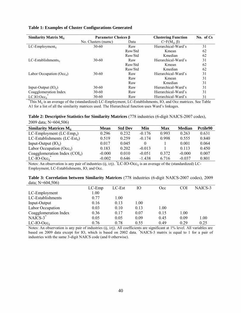
40

Table 1: Examples of Cluster Configurations Generated

Similarity Matrix Mij Parameter Choices β Clustering Function No. of Cs

No. Clusters (numc) Data C=F(Mij, β) LC-Employmentij 30-60 Raw Hierarchical-Ward’s 31

Raw/Std Kmean 62 Raw/Std Kmedian 62 LC-Establishmentsij 30-60 Raw Hierarchical-Ward’s 31

Raw/Std Kmean 62

Raw/Std Kmedian 62 Labor Occupation (Occij) 30-60 Raw Hierarchical-Ward’s 31

Raw Kmean 31 Raw Kmedian 31 Input-Output (IOij) 30-60 Raw Hierarchical-Ward’s 31 Coagglomeration Index 30-60 Raw Hierarchical-Ward’s 31 LC-IO-Occij

* 30-60 Raw Hierarchical-Ward’s 31

*This Mij is an average of the (standardized) LC-Employment, LC-Establishments, IO, and Occ matrices. See Table A1 for a list of all the similarity matrices used. The Hierarchical function uses Ward’s linkages. Table 2: Descriptive Statistics for Similarity Matrices (778 industries (6-digit NAICS-2007 codes), 2009 data; N=604,506) Similarity Matrices Mij Mean Std Dev Min Max Median Pctile90

LC-Employment (LC-Empij) 0.296 0.232 -0.176 0.993 0.263 0.631 LC-Establishments (LC-Estij) 0.519 0.259 -0.174 0.998 0.555 0.840 Input-Output (IOij) 0.017 0.045 0 1 0.001 0.064 Labor Occupation (Occij) 0.183 0.202 -0.013 1 0.113 0.450 Coagglomeration Index (COIij) -0.000 0.010 -0.051 0.372 -0.000 0.007 LC-IO-Occij

* -0.002 0.646 -1.438 6.716 -0.037 0.801 Notes: An observation is any pair of industries (ij, i≠j). *LC-IO-Occij is an average of the (standardized) LC-Employment, LC-Establishments, IO, and Occ.

Table 3: Correlation between Similarity Matrices (778 industries (6-digit NAICS-2007 codes), 2009 data; N=604,506)

LC-Emp LC-Est IO Occ COI NAICS-3

LC-Employment 1.00

LC-Establishments 0.77 1.00

Input-Output 0.16 0.13 1.00

Labor Occupation 0.03 0.10 0.13 1.00

Coagglomeration Index 0.36 0.17 0.07 0.15 1.00 NAICS-3* 0.05 0.05 0.09 0.45 0.09 1.00 LC-IO-Occij 0.76 0.78 0.55 0.49 0.29 0.25 Notes: An observation is any pair of industries (ij, i≠j). All coefficients are significant at 1% level. All variables are based on 2009 data except for IO, which is based on 2002 data. *NAICS-3 matrix is equal to 1 for a pair of industries with the same 3-digit NAICS code (and 0 otherwise).

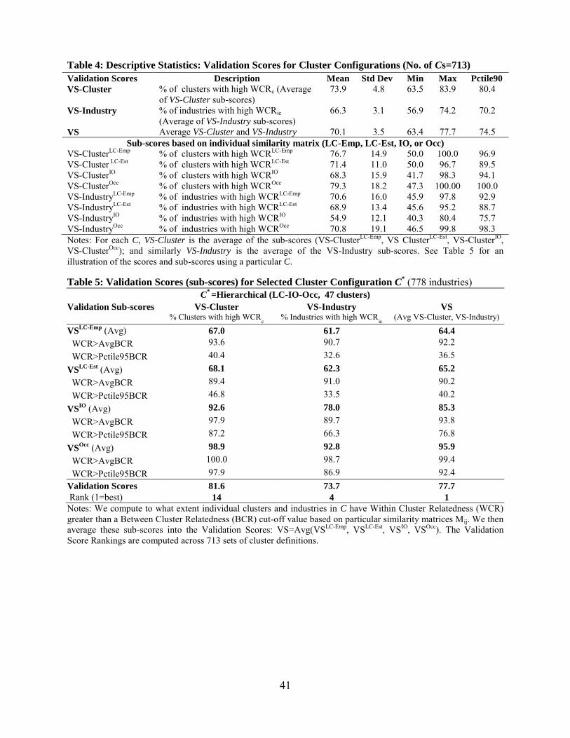
41

Table 4: Descriptive Statistics: Validation Scores for Cluster Configurations (No. of Cs=713)

Validation Scores Description Mean Std Dev Min Max Pctile90

VS-Cluster % of clusters with high WCRc (Average of VS-Cluster sub-scores)

73.9

4.8

63.5

83.9

80.4

VS-Industry % of industries with high WCRic

(Average of VS-Industry sub-scores)

66.3

3.1

56.9

74.2

70.2

VS Average VS-Cluster and VS-Industry 70.1 3.5 63.4 77.7 74.5 Sub-scores based on individual similarity matrix (LC-Emp, LC-Est, IO, or Occ)

VS-ClusterLC-Emp % of clusters with high WCRLC-Emp 76.7 14.9 50.0 100.0 96.9

VS-Cluster LC-Est % of clusters with high WCRLC-Est 71.4 11.0 50.0 96.7 89.5

VS-ClusterIO % of clusters with high WCRIO 68.3 15.9 41.7 98.3 94.1

VS-ClusterOcc % of clusters with high WCROcc 79.3 18.2 47.3 100.00 100.0

VS-IndustryLC-Emp % of industries with high WCRLC-Emp 70.6 16.0 45.9 97.8 92.9

VS-IndustryLC-Est % of industries with high WCRLC-Est 68.9 13.4 45.6 95.2 88.7

VS-IndustryIO % of industries with high WCRIO 54.9 12.1 40.3 80.4 75.7

VS-IndustryOcc % of industries with high WCROcc 70.8 19.1 46.5 99.8 98.3

Notes: For each C, VS-Cluster is the average of the sub-scores (VS-ClusterLC-Emp, VS ClusterLC-Est, VS-ClusterIO, VS-ClusterOcc); and similarly VS-Industry is the average of the VS-Industry sub-scores. See Table 5 for an illustration of the scores and sub-scores using a particular C.

Table 5: Validation Scores (sub-scores) for Selected Cluster Configuration C* (778 industries)

C* =Hierarchical (LC-IO-Occ, 47 clusters)

Validation Sub-scores VS-Cluster % Clusters with high WCRc

VS-Industry % Industries with high WCRic

VS (Avg VS-Cluster, VS-Industry)

VSLC-Emp

(Avg) 67.0 61.7 64.4

WCR>AvgBCR 93.6 90.7 92.2 WCR>Pctile95BCR 40.4 32.6 36.5 VS

LC-Est (Avg) 68.1 62.3 65.2

WCR>AvgBCR 89.4 91.0 90.2 WCR>Pctile95BCR 46.8 33.5 40.2 VS

IO (Avg) 92.6 78.0 85.3

WCR>AvgBCR 97.9 89.7 93.8 WCR>Pctile95BCR 87.2 66.3 76.8 VS

Occ (Avg) 98.9 92.8 95.9

WCR>AvgBCR 100.0 98.7 99.4 WCR>Pctile95BCR 97.9 86.9 92.4 Validation Scores 81.6 73.7 77.7

Rank (1=best) 14 4 1

Notes: We compute to what extent individual clusters and industries in C have Within Cluster Relatedness (WCR) greater than a Between Cluster Relatedness (BCR) cut-off value based on particular similarity matrices Mij. We then average these sub-scores into the Validation Scores: VS=Avg(VSLC-Emp, VSLC-Est, VSIO, VSOcc). The Validation Score Rankings are computed across 713 sets of cluster definitions.

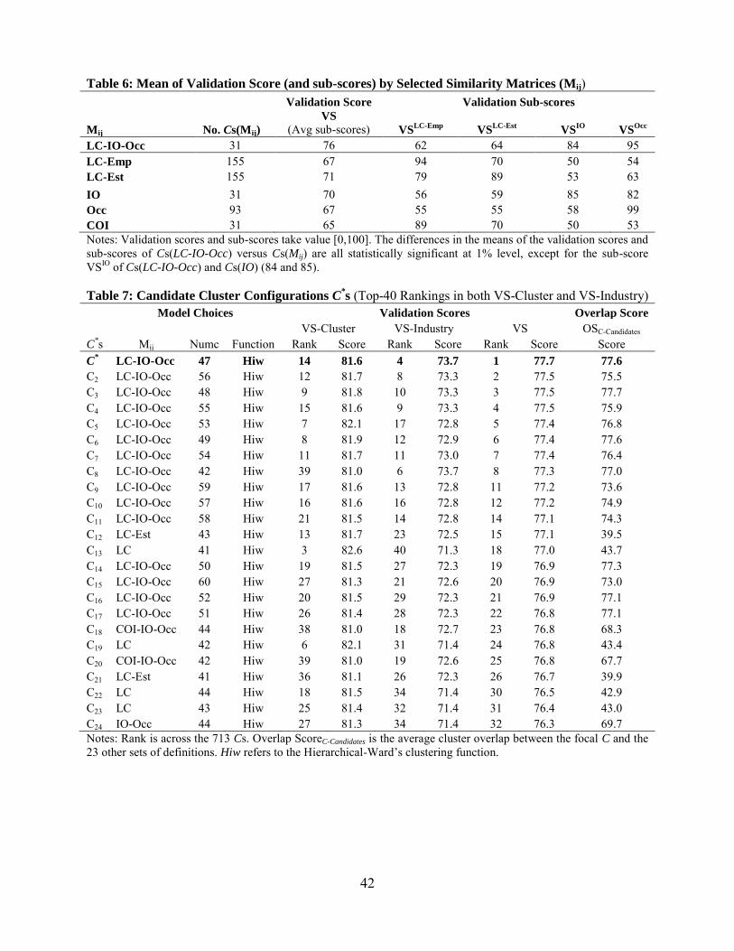
42

Table 6: Mean of Validation Score (and sub-scores) by Selected Similarity Matrices (Mij) Validation Score Validation Sub-scores

Mij No. Cs(Mij)

VS

(Avg sub-scores) VSLC-Emp

VSLC-Est

VSIO

VSOcc

LC-IO-Occ 31 76 62 64 84 95 LC-Emp 155 67 94 70 50 54 LC-Est 155 71 79 89 53 63 IO 31 70 56 59 85 82 Occ 93 67 55 55 58 99 COI 31 65 89 70 50 53 Notes: Validation scores and sub-scores take value [0,100]. The differences in the means of the validation scores and sub-scores of Cs(LC-IO-Occ) versus Cs(Mij) are all statistically significant at 1% level, except for the sub-score VSIO of Cs(LC-IO-Occ) and Cs(IO) (84 and 85). Table 7: Candidate Cluster Configurations C

*s (Top-40 Rankings in both VS-Cluster and VS-Industry)

Model Choices Validation Scores Overlap Score

VS-Cluster VS-Industry VS OSC-Candidates

C*s Mij Numc Function Rank Score Rank Score Rank Score Score

C* LC-IO-Occ 47 Hiw 14 81.6 4 73.7 1 77.7 77.6

C2 LC-IO-Occ 56 Hiw 12 81.7 8 73.3 2 77.5 75.5 C3 LC-IO-Occ 48 Hiw 9 81.8 10 73.3 3 77.5 77.7 C4 LC-IO-Occ 55 Hiw 15 81.6 9 73.3 4 77.5 75.9 C5 LC-IO-Occ 53 Hiw 7 82.1 17 72.8 5 77.4 76.8 C6 LC-IO-Occ 49 Hiw 8 81.9 12 72.9 6 77.4 77.6 C7 LC-IO-Occ 54 Hiw 11 81.7 11 73.0 7 77.4 76.4 C8 LC-IO-Occ 42 Hiw 39 81.0 6 73.7 8 77.3 77.0 C9 LC-IO-Occ 59 Hiw 17 81.6 13 72.8 11 77.2 73.6 C10 LC-IO-Occ 57 Hiw 16 81.6 16 72.8 12 77.2 74.9 C11 LC-IO-Occ 58 Hiw 21 81.5 14 72.8 14 77.1 74.3 C12 LC-Est 43 Hiw 13 81.7 23 72.5 15 77.1 39.5 C13 LC 41 Hiw 3 82.6 40 71.3 18 77.0 43.7 C14 LC-IO-Occ 50 Hiw 19 81.5 27 72.3 19 76.9 77.3 C15 LC-IO-Occ 60 Hiw 27 81.3 21 72.6 20 76.9 73.0 C16 LC-IO-Occ 52 Hiw 20 81.5 29 72.3 21 76.9 77.1 C17 LC-IO-Occ 51 Hiw 26 81.4 28 72.3 22 76.8 77.1 C18 COI-IO-Occ 44 Hiw 38 81.0 18 72.7 23 76.8 68.3 C19 LC 42 Hiw 6 82.1 31 71.4 24 76.8 43.4 C20 COI-IO-Occ 42 Hiw 39 81.0 19 72.6 25 76.8 67.7 C21 LC-Est 41 Hiw 36 81.1 26 72.3 26 76.7 39.9 C22 LC 44 Hiw 18 81.5 34 71.4 30 76.5 42.9 C23 LC 43 Hiw 25 81.4 32 71.4 31 76.4 43.0 C24 IO-Occ 44 Hiw 27 81.3 34 71.4 32 76.3 69.7 Notes: Rank is across the 713 Cs. Overlap ScoreC-Candidates is the average cluster overlap between the focal C and the 23 other sets of definitions. Hiw refers to the Hierarchical-Ward’s clustering function.

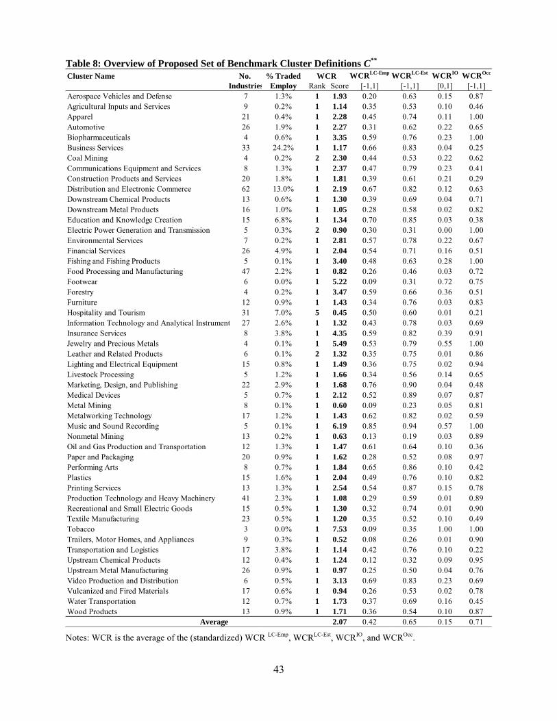
43

Table 8: Overview of Proposed Set of Benchmark Cluster Definitions C**

Notes: WCR is the average of the (standardized) WCR LC-Emp, WCRLC-Est, WCRIO, and WCROcc.

Cluster Name No. % Traded WCRLC-Emp

WCRLC-Est

WCRIO

WCROcc

Industries Employ Rank Score [-1,1] [-1,1] [0,1] [-1,1]Aerospace Vehicles and Defense 7 1.3% 1 1.93 0.20 0.63 0.15 0.87Agricultural Inputs and Services 9 0.2% 1 1.14 0.35 0.53 0.10 0.46Apparel 21 0.4% 1 2.28 0.45 0.74 0.11 1.00Automotive 26 1.9% 1 2.27 0.31 0.62 0.22 0.65Biopharmaceuticals 4 0.6% 1 3.35 0.59 0.76 0.23 1.00Business Services 33 24.2% 1 1.17 0.66 0.83 0.04 0.25Coal Mining 4 0.2% 2 2.30 0.44 0.53 0.22 0.62Communications Equipment and Services 8 1.3% 1 2.37 0.47 0.79 0.23 0.41Construction Products and Services 20 1.8% 1 1.81 0.39 0.61 0.21 0.29Distribution and Electronic Commerce 62 13.0% 1 2.19 0.67 0.82 0.12 0.63Downstream Chemical Products 13 0.6% 1 1.30 0.39 0.69 0.04 0.71Downstream Metal Products 16 1.0% 1 1.05 0.28 0.58 0.02 0.82Education and Knowledge Creation 15 6.8% 1 1.34 0.70 0.85 0.03 0.38Electric Power Generation and Transmission 5 0.3% 2 0.90 0.30 0.31 0.00 1.00Environmental Services 7 0.2% 1 2.81 0.57 0.78 0.22 0.67Financial Services 26 4.9% 1 2.04 0.54 0.71 0.16 0.51Fishing and Fishing Products 5 0.1% 1 3.40 0.48 0.63 0.28 1.00Food Processing and Manufacturing 47 2.2% 1 0.82 0.26 0.46 0.03 0.72Footwear 6 0.0% 1 5.22 0.09 0.31 0.72 0.75Forestry 4 0.2% 1 3.47 0.59 0.66 0.36 0.51Furniture 12 0.9% 1 1.43 0.34 0.76 0.03 0.83Hospitality and Tourism 31 7.0% 5 0.45 0.50 0.60 0.01 0.21Information Technology and Analytical Instruments 27 2.6% 1 1.32 0.43 0.78 0.03 0.69Insurance Services 8 3.8% 1 4.35 0.59 0.82 0.39 0.91Jewelry and Precious Metals 4 0.1% 1 5.49 0.53 0.79 0.55 1.00Leather and Related Products 6 0.1% 2 1.32 0.35 0.75 0.01 0.86Lighting and Electrical Equipment 15 0.8% 1 1.49 0.36 0.75 0.02 0.94Livestock Processing 5 1.2% 1 1.66 0.34 0.56 0.14 0.65Marketing, Design, and Publishing 22 2.9% 1 1.68 0.76 0.90 0.04 0.48Medical Devices 5 0.7% 1 2.12 0.52 0.89 0.07 0.87Metal Mining 8 0.1% 1 0.60 0.09 0.23 0.05 0.81Metalworking Technology 17 1.2% 1 1.43 0.62 0.82 0.02 0.59Music and Sound Recording 5 0.1% 1 6.19 0.85 0.94 0.57 1.00Nonmetal Mining 13 0.2% 1 0.63 0.13 0.19 0.03 0.89Oil and Gas Production and Transportation 12 1.3% 1 1.47 0.61 0.64 0.10 0.36Paper and Packaging 20 0.9% 1 1.62 0.28 0.52 0.08 0.97Performing Arts 8 0.7% 1 1.84 0.65 0.86 0.10 0.42Plastics 15 1.6% 1 2.04 0.49 0.76 0.10 0.82Printing Services 13 1.3% 1 2.54 0.54 0.87 0.15 0.78Production Technology and Heavy Machinery 41 2.3% 1 1.08 0.29 0.59 0.01 0.89Recreational and Small Electric Goods 15 0.5% 1 1.30 0.32 0.74 0.01 0.90Textile Manufacturing 23 0.5% 1 1.20 0.35 0.52 0.10 0.49Tobacco 3 0.0% 1 7.53 0.09 0.35 1.00 1.00Trailers, Motor Homes, and Appliances 9 0.3% 1 0.52 0.08 0.26 0.01 0.90Transportation and Logistics 17 3.8% 1 1.14 0.42 0.76 0.10 0.22Upstream Chemical Products 12 0.4% 1 1.24 0.12 0.32 0.09 0.95Upstream Metal Manufacturing 26 0.9% 1 0.97 0.25 0.50 0.04 0.76Video Production and Distribution 6 0.5% 1 3.13 0.69 0.83 0.23 0.69Vulcanized and Fired Materials 17 0.6% 1 0.94 0.26 0.53 0.02 0.78Water Transportation 12 0.7% 1 1.73 0.37 0.69 0.16 0.45Wood Products 13 0.9% 1 1.71 0.36 0.54 0.10 0.87

Average 2.07 0.42 0.65 0.15 0.71

WCR

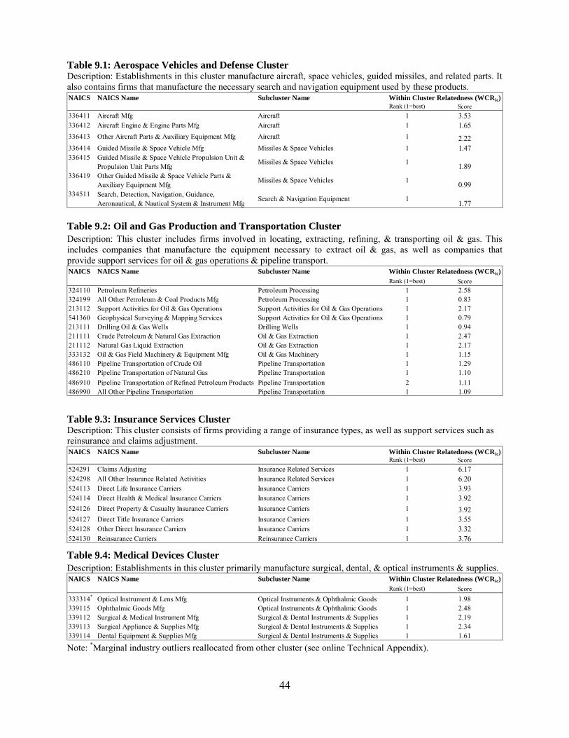
44

Table 9.1: Aerospace Vehicles and Defense Cluster Description: Establishments in this cluster manufacture aircraft, space vehicles, guided missiles, and related parts. It also contains firms that manufacture the necessary search and navigation equipment used by these products.

Table 9.2: Oil and Gas Production and Transportation Cluster

Description: This cluster includes firms involved in locating, extracting, refining, & transporting oil & gas. This includes companies that manufacture the equipment necessary to extract oil & gas, as well as companies that provide support services for oil & gas operations & pipeline transport.

Table 9.3: Insurance Services Cluster Description: This cluster consists of firms providing a range of insurance types, as well as support services such as reinsurance and claims adjustment.

Table 9.4: Medical Devices Cluster

Description: Establishments in this cluster primarily manufacture surgical, dental, & optical instruments & supplies.

Note: *Marginal industry outliers reallocated from other cluster (see online Technical Appendix).

NAICS NAICS Name Subcluster Name Within Cluster Relatedness (WCRic)

Rank (1=best) Score336411 Aircraft Mfg Aircraft 1 3.53336412 Aircraft Engine & Engine Parts Mfg Aircraft 1 1.65336413 Other Aircraft Parts & Auxiliary Equipment Mfg Aircraft 1 2.22336414 Guided Missile & Space Vehicle Mfg Missiles & Space Vehicles 1 1.47336415 Guided Missile & Space Vehicle Propulsion Unit &

Propulsion Unit Parts MfgMissiles & Space Vehicles 1 1.89

336419 Other Guided Missile & Space Vehicle Parts & Auxiliary Equipment Mfg

Missiles & Space Vehicles 1 0.99334511 Search, Detection, Navigation, Guidance,

Aeronautical, & Nautical System & Instrument MfgSearch & Navigation Equipment 1 1.77

NAICS NAICS Name Subcluster Name Within Cluster Relatedness (WCRic)

Rank (1=best) Score324110 Petroleum Refineries Petroleum Processing 1 2.58324199 All Other Petroleum & Coal Products Mfg Petroleum Processing 1 0.83213112 Support Activities for Oil & Gas Operations Support Activities for Oil & Gas Operations 1 2.17541360 Geophysical Surveying & Mapping Services Support Activities for Oil & Gas Operations 1 0.79213111 Drilling Oil & Gas Wells Drilling Wells 1 0.94211111 Crude Petroleum & Natural Gas Extraction Oil & Gas Extraction 1 2.47211112 Natural Gas Liquid Extraction Oil & Gas Extraction 1 2.17333132 Oil & Gas Field Machinery & Equipment Mfg Oil & Gas Machinery 1 1.15486110 Pipeline Transportation of Crude Oil Pipeline Transportation 1 1.29486210 Pipeline Transportation of Natural Gas Pipeline Transportation 1 1.10486910 Pipeline Transportation of Refined Petroleum Products Pipeline Transportation 2 1.11486990 All Other Pipeline Transportation Pipeline Transportation 1 1.09

NAICS NAICS Name Subcluster Name Within Cluster Relatedness (WCRic)Rank (1=best) Score

524291 Claims Adjusting Insurance Related Services 1 6.17524298 All Other Insurance Related Activities Insurance Related Services 1 6.20524113 Direct Life Insurance Carriers Insurance Carriers 1 3.93524114 Direct Health & Medical Insurance Carriers Insurance Carriers 1 3.92524126 Direct Property & Casualty Insurance Carriers Insurance Carriers 1 3.92524127 Direct Title Insurance Carriers Insurance Carriers 1 3.55524128 Other Direct Insurance Carriers Insurance Carriers 1 3.32524130 Reinsurance Carriers Reinsurance Carriers 1 3.76

NAICS NAICS Name Subcluster Name Within Cluster Relatedness (WCRic)

Rank (1=best) Score

333314* Optical Instrument & Lens Mfg Optical Instruments & Ophthalmic Goods 1 1.98339115 Ophthalmic Goods Mfg Optical Instruments & Ophthalmic Goods 1 2.48339112 Surgical & Medical Instrument Mfg Surgical & Dental Instruments & Supplies 1 2.19339113 Surgical Appliance & Supplies Mfg Surgical & Dental Instruments & Supplies 1 2.34339114 Dental Equipment & Supplies Mfg Surgical & Dental Instruments & Supplies 1 1.61

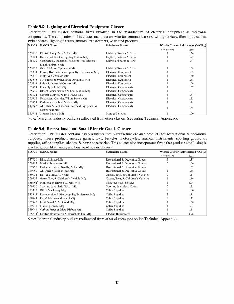
45

Table 9.5: Lighting and Electrical Equipment Cluster

Description: This cluster contains firms involved in the manufacture of electrical equipment & electronic components. The companies in this cluster manufacture wire for communications, wiring devices, fiber-optic cables, switchboards, lighting fixtures, motors, transformers, & related products.

Note: *Marginal industry outliers reallocated from other clusters (see online Technical Appendix). Table 9.6: Recreational and Small Electric Goods Cluster

Description: This cluster contains establishments that manufacture end-use products for recreational & decorative purposes. These products include games, toys, bicycles, motorcycles, musical instruments, sporting goods, art supplies, office supplies, shades, & home accessories. This cluster also incorporates firms that produce small, simple electric goods like hairdryers, fans, & office machinery.

Note: *Marginal industry outliers reallocated from other clusters (see online Technical Appendix).

NAICS NAICS Name Subcluster Name Within Cluster Relatedness (WCRic)

Rank (1=best) Score

335110 Electric Lamp Bulb & Part Mfg Lighting Fixtures & Parts 1 1.34335121 Residential Electric Lighting Fixture Mfg Lighting Fixtures & Parts 1 1.77335122 Commercial, Industrial, & Institutional Electric

Lighting Fixture MfgLighting Fixtures & Parts 1 1.77

335129 Other Lighting Equipment Mfg Lighting Fixtures & Parts 1 1.68335311 Power, Distribution, & Specialty Transformer Mfg Electrical Equipment 1 1.62335312 Motor & Generator Mfg Electrical Equipment 1 1.30335313 Switchgear & Switchboard Apparatus Mfg Electrical Equipment 1 1.48335314 Relay & Industrial Control Mfg Electrical Equipment 1 1.64335921 Fiber Optic Cable Mfg Electrical Components 1 1.39335929 Other Communication & Energy Wire Mfg Electrical Components 1 1.61335931 Current-Carrying Wiring Device Mfg Electrical Components 1 1.67335932 Noncurrent-Carrying Wiring Device Mfg Electrical Components 1 1.23335991 Carbon & Graphite Product Mfg Electrical Components 1 1.15335999* All Other Miscellaneous Electrical Equipment &

Component MfgElectrical Components 1 1.65

335911 Storage Battery Mfg Storage Batteries 1 1.00

NAICS NAICS Name Subcluster Name Within Cluster Relatedness (WCRic)

Rank (1=best) Score

337920 Blind & Shade Mfg Recreational & Decorative Goods 3 1.37339992 Musical Instrument Mfg Recreational & Decorative Goods 3 1.60339993 Fastener, Button, Needle, & Pin Mfg Recreational & Decorative Goods 3 1.37339999 All Other Miscellaneous Mfg Recreational & Decorative Goods 1 1.58339931 Doll & Stuffed Toy Mfg Games, Toys, & Children’s Vehicles 2 1.17339932 Game, Toy, & Children’s Vehicle Mfg Games, Toys, & Children’s Vehicles 1 1.44336991* Motorcycle, Bicycle, & Parts Mfg Motorcycles & Bicycles 1 0.94339920 Sporting & Athletic Goods Mfg Sporting & Athletic Goods 3 1.25333313 Office Machinery Mfg Office Supplies 4 1.00333315* Photographic & Photocopying Equipment Mfg Office Supplies 3 1.35339941 Pen & Mechanical Pencil Mfg Office Supplies 2 1.43339942 Lead Pencil & Art Good Mfg Office Supplies 1 1.50339943 Marking Device Mfg Office Supplies 1 1.61339944 Carbon Paper & Inked Ribbon Mfg Office Supplies 1 1.11335211* Electric Housewares & Household Fan Mfg Electric Housewares 1 0.78

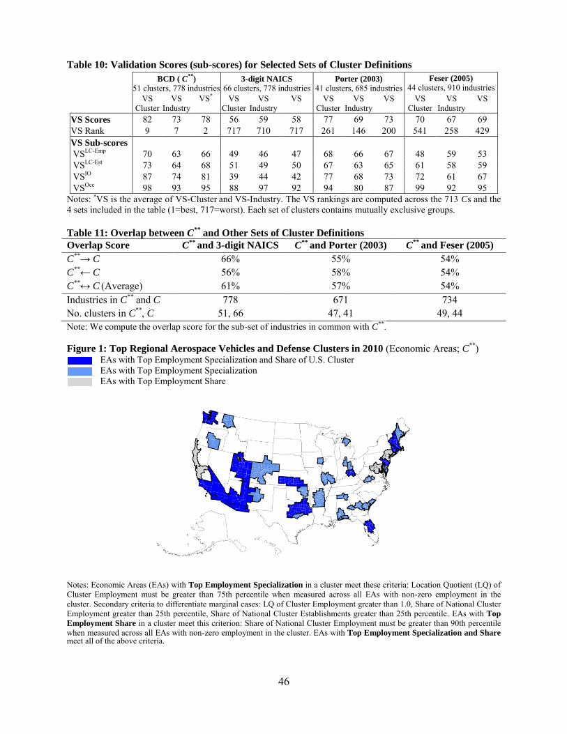
46

Table 10: Validation Scores (sub-scores) for Selected Sets of Cluster Definitions

BCD ( C**

)

51 clusters, 778 industries

3-digit NAICS

66 clusters, 778 industries Porter (2003)

41 clusters, 685 industries

Feser (2005)

44 clusters, 910 industries

VS Cluster

VS Industry

VS*

VS

Cluster VS

Industry VS

VS

Cluster VS

Industry VS

VS

Cluster VS

Industry VS

VS Scores 82 73 78 56 59 58 77 69 73 70 67 69 VS Rank 9 7 2 717 710 717 261 146 200 541 258 429 VS Sub-scores VSLC-Emp 70 63 66 49 46 47 68 66 67 48 59 53 VSLC-Est 73 64 68 51 49 50 67 63 65 61 58 59 VSIO 87 74 81 39 44 42 77 68 73 72 61 67 VSOcc 98 93 95 88 97 92 94 80 87 99 92 95

Notes: *VS is the average of VS-Cluster and VS-Industry. The VS rankings are computed across the 713 Cs and the 4 sets included in the table (1=best, 717=worst). Each set of clusters contains mutually exclusive groups.

Table 11: Overlap between C**

and Other Sets of Cluster Definitions

Overlap Score C** and 3-digit NAICS C** and Porter (2003) C**

and Feser (2005) C

**→ C 66% 55% 54% C

**← C 56% 58% 54% C

**↔ C (Average) 61% 57% 54% Industries in C** and C 778 671 734 No. clusters in C**, C 51, 66 47, 41 49, 44 Note: We compute the overlap score for the sub-set of industries in common with C**. Figure 1: Top Regional Aerospace Vehicles and Defense Clusters in 2010 (Economic Areas; C**)

EAs with Top Employment Specialization and Share of U.S. Cluster EAs with Top Employment Specialization EAs with Top Employment Share

Notes: Economic Areas (EAs) with Top Employment Specialization in a cluster meet these criteria: Location Quotient (LQ) of Cluster Employment must be greater than 75th percentile when measured across all EAs with non-zero employment in the cluster. Secondary criteria to differentiate marginal cases: LQ of Cluster Employment greater than 1.0, Share of National Cluster Employment greater than 25th percentile, Share of National Cluster Establishments greater than 25th percentile. EAs with Top

Employment Share in a cluster meet this criterion: Share of National Cluster Employment must be greater than 90th percentile when measured across all EAs with non-zero employment in the cluster. EAs with Top Employment Specialization and Share meet all of the above criteria.

47

Appendix A

Table A1: Similarity Matrices Used to Generate Sets of Cluster Definitions Cs

Similarity Matrix No. of Cs Type of Mij Definition

LC-Emp 155 Unidimensional Locational Correlation of employment [-1, 1] LC-Est 155 Unidimensional Locational Correlation of establishments [-1, 1] IO 31 Unidimensional Input-Output link [0, 1] Occ 93 Unidimensional Labor Occupation link [-1, 1] COI 31 Unidimensional Coagglomeration Index LC-IO-Occ 31 Multidimensional Average of (standardized) LC-Emp, LC-Est, IO, Occ COI-IO-Occ 31 Multidimensional Average of (standardized) COI, IO, Occ LC 31 Multidimensional Average of LC-Emp, LC-Est IO-Occ 31 Multidimensional Average of (standardized) IO, Occ LC-Emp-IO 31 Multidimensional Average of (standardized) LC-Emp, IO LC-Est-IO 31 Multidimensional Average of (standardized) LC-Est, IO LC-Emp-Occ 31 Multidimensional Average of LC-Emp, Occ LC-Est-Occ 31 Multidimensional Average of LC-Est, Occ

An online Technical Appendix, with a detailed cluster-by-cluster overview of the proposed set of benchmark cluster definitions (C**), may be accessed here.