Default and Recovery Implicit in the Term Structure of ...web.stanford.edu/~kenneths/sovcds.pdf ·...
40
THE JOURNAL OF FINANCE • VOL. LXIII, NO. 5 • OCTOBER 2008 Default and Recovery Implicit in the Term Structure of Sovereign CDS Spreads JUN PAN and KENNETH J. SINGLETON ∗ ABSTRACT This paper explores the nature of default arrival and recovery implicit in the term structures of sovereign CDS spreads. We argue that term structures of spreads re- veal not only the arrival rates of credit events (λ Q ), but also the loss rates given credit events. Applying our framework to Mexico, Turkey, and Korea, we show that a single-factor model with λ Q following a lognormal process captures most of the variation in the term structures of spreads. The risk premiums associated with un- predictable variation in λ Q are found to be economically significant and co-vary impor- tantly with several economic measures of global event risk, financial market volatility, and macroeconomic policy. THE BURGEONING MARKET FOR SOVEREIGN CREDIT DEFAULT SWAPS (CDS) contracts of- fers a nearly unique window for viewing investors’ risk-neutral probabilities of major credit events impinging on sovereign issuers, and their risk-neutral losses of principal in the event of a restructuring or repudiation of external debts. In contrast to many “emerging market” sovereign bonds, sovereign CDS contracts are designed without complex guarantees or embedded options. Trad- ing activity in the CDS contracts of several sovereign issuers has developed to the point that they are more liquid than many of the underlying bonds. Moreover, in contrast to the corporate CDS market, where trading has been concentrated largely in the 5-year maturity contract, CDS contracts at several maturity points between 1 and 10 years have been actively traded for several years. As such, a full term structure of CDS spreads is available for inferring default and recovery information from market data. This paper explores in depth the time-series properties of the risk-neutral mean arrival rates of credit events (λ Q ) implicit in the term structure of sovereign CDS spreads. Applying our framework to Mexico, Turkey, and Korea, three countries with different geopolitical characteristics and credit ratings, we ∗ Pan is with the MIT Sloan School of Management and NBER. Singleton is with the Graduate School of Business, Stanford University and NBER. We have benefited from discussions with Antje Berndt, Darrell Duffie, Michael Johannes, Jun Liu, Francis Longstaff, Roberto Rigobon; seminar participants at Chicago, Columbia, CREST, Duke, USC, UCLA, University of Michigan, the 2005 NBER IASE workshop, the November 2005 NBER Asset Pricing meeting, the 2006 AFA Meet- ings, AQR, the 2007 Fed conference on credit risk and credit derivatives; and the comments of two anonymous referees. Scott Joslin provided excellent research assistance. We are grateful for finan- cial support from the Gifford Fong Associates Fund at the Graduate School of Business, Stanford University and from the MIT Laboratory for Financial Engineering. 2345
Transcript of Default and Recovery Implicit in the Term Structure of ...web.stanford.edu/~kenneths/sovcds.pdf ·...

THE JOURNAL OF FINANCE • VOL. LXIII, NO. 5 • OCTOBER 2008
Default and Recovery Implicit in the TermStructure of Sovereign CDS Spreads
JUN PAN and KENNETH J. SINGLETON∗
ABSTRACT
This paper explores the nature of default arrival and recovery implicit in the termstructures of sovereign CDS spreads. We argue that term structures of spreads re-veal not only the arrival rates of credit events (λQ), but also the loss rates givencredit events. Applying our framework to Mexico, Turkey, and Korea, we show thata single-factor model with λQ following a lognormal process captures most of thevariation in the term structures of spreads. The risk premiums associated with un-predictable variation in λQ are found to be economically significant and co-vary impor-tantly with several economic measures of global event risk, financial market volatility,and macroeconomic policy.
THE BURGEONING MARKET FOR SOVEREIGN CREDIT DEFAULT SWAPS (CDS) contracts of-fers a nearly unique window for viewing investors’ risk-neutral probabilitiesof major credit events impinging on sovereign issuers, and their risk-neutrallosses of principal in the event of a restructuring or repudiation of externaldebts. In contrast to many “emerging market” sovereign bonds, sovereign CDScontracts are designed without complex guarantees or embedded options. Trad-ing activity in the CDS contracts of several sovereign issuers has developedto the point that they are more liquid than many of the underlying bonds.Moreover, in contrast to the corporate CDS market, where trading has beenconcentrated largely in the 5-year maturity contract, CDS contracts at severalmaturity points between 1 and 10 years have been actively traded for severalyears. As such, a full term structure of CDS spreads is available for inferringdefault and recovery information from market data.
This paper explores in depth the time-series properties of the risk-neutralmean arrival rates of credit events (λQ) implicit in the term structure ofsovereign CDS spreads. Applying our framework to Mexico, Turkey, and Korea,three countries with different geopolitical characteristics and credit ratings, we
∗Pan is with the MIT Sloan School of Management and NBER. Singleton is with the GraduateSchool of Business, Stanford University and NBER. We have benefited from discussions with AntjeBerndt, Darrell Duffie, Michael Johannes, Jun Liu, Francis Longstaff, Roberto Rigobon; seminarparticipants at Chicago, Columbia, CREST, Duke, USC, UCLA, University of Michigan, the 2005NBER IASE workshop, the November 2005 NBER Asset Pricing meeting, the 2006 AFA Meet-ings, AQR, the 2007 Fed conference on credit risk and credit derivatives; and the comments of twoanonymous referees. Scott Joslin provided excellent research assistance. We are grateful for finan-cial support from the Gifford Fong Associates Fund at the Graduate School of Business, StanfordUniversity and from the MIT Laboratory for Financial Engineering.
2345
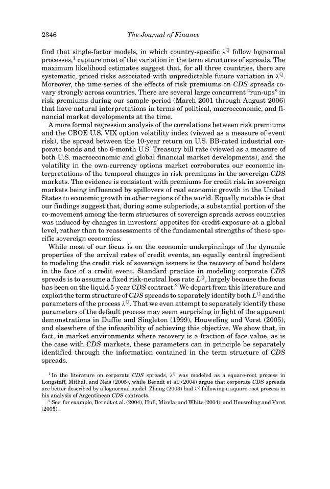
2346 The Journal of Finance
find that single-factor models, in which country-specific λQ follow lognormalprocesses,1 capture most of the variation in the term structures of spreads. Themaximum likelihood estimates suggest that, for all three countries, there aresystematic, priced risks associated with unpredictable future variation in λQ.Moreover, the time-series of the effects of risk premiums on CDS spreads co-vary strongly across countries. There are several large concurrent “run-ups” inrisk premiums during our sample period (March 2001 through August 2006)that have natural interpretations in terms of political, macroeconomic, and fi-nancial market developments at the time.
A more formal regression analysis of the correlations between risk premiumsand the CBOE U.S. VIX option volatility index (viewed as a measure of eventrisk), the spread between the 10-year return on U.S. BB-rated industrial cor-porate bonds and the 6-month U.S. Treasury bill rate (viewed as a measure ofboth U.S. macroeconomic and global financial market developments), and thevolatility in the own-currency options market corroborates our economic in-terpretations of the temporal changes in risk premiums in the sovereign CDSmarkets. The evidence is consistent with premiums for credit risk in sovereignmarkets being influenced by spillovers of real economic growth in the UnitedStates to economic growth in other regions of the world. Equally notable is thatour findings suggest that, during some subperiods, a substantial portion of theco-movement among the term structures of sovereign spreads across countrieswas induced by changes in investors’ appetites for credit exposure at a globallevel, rather than to reassessments of the fundamental strengths of these spe-cific sovereign economies.
While most of our focus is on the economic underpinnings of the dynamicproperties of the arrival rates of credit events, an equally central ingredientto modeling the credit risk of sovereign issuers is the recovery of bond holdersin the face of a credit event. Standard practice in modeling corporate CDSspreads is to assume a fixed risk-neutral loss rate LQ, largely because the focushas been on the liquid 5-year CDS contract.2 We depart from this literature andexploit the term structure of CDS spreads to separately identify both LQ and theparameters of the process λQ. That we even attempt to separately identify theseparameters of the default process may seem surprising in light of the apparentdemonstrations in Duffie and Singleton (1999), Houweling and Vorst (2005),and elsewhere of the infeasibility of achieving this objective. We show that, infact, in market environments where recovery is a fraction of face value, as isthe case with CDS markets, these parameters can in principle be separatelyidentified through the information contained in the term structure of CDSspreads.
1 In the literature on corporate CDS spreads, λQ was modeled as a square-root process inLongstaff, Mithal, and Neis (2005), while Berndt et al. (2004) argue that corporate CDS spreadsare better described by a lognormal model. Zhang (2003) had λQ following a square-root process inhis analysis of Argentinean CDS contracts.
2 See, for example, Berndt et al. (2004), Hull, Mirela, and White (2004), and Houweling and Vorst(2005).

Default and Recovery Implicit in Term Structure of Sovereign CDS 2347
The maximum likelihood (ML) estimates of the parameters governing λQ
imply that its risk-neutral (Q) distribution shows very little mean reversionand, in fact, in some cases λQ is Q-explosive. In contrast, the historical data-generating process (P) for λQ shows substantial mean reversion, consistent withthe P-stationarity of CDS spreads. This large difference between the propertiesof λQ under the Q and P measures implies, within the context of our models,that an economically important systematic risk is being priced in the CDSmarket.
Our ML estimates are obtained both with fixed LQ at the market conven-tion 0.75, and by searching over LQ as a free parameter. In the latter case, thelikelihood functions call for much smaller values of LQ for Mexico and Turkey,more in the region of 0.25, and also slower rates of P-mean reversion of λQ.An extensive Monte Carlo analysis of the small-sample distributions of vari-ous moments reveals that many features of the implied distributions of CDSspreads for Mexico and Turkey are similar across the cases of LQ equal to 0.75or 0.25. For our model formulation and sample ML estimates, it is only overlong horizons—for most of our countries, longer than our sample periods—thatthe differences in P-mean reversion in the two cases manifest themselves. Thisobservation, combined with our finding that the unconstrained estimate of LQ
for Korea is similar to the market convention of 0.75, leads us to set LQ = 0.75for our analysis of risk premiums.
Throughout our analysis we maintain the assumption that a single risk factorunderlies the temporal variation in λQ, consistent with most previous studiesof CDS spreads that have allowed for a stochastic arrival rate of credit events.In the case of our sovereign data, this focus is motivated by the high degree ofco-movement among spreads across the maturity spectrum within each coun-try. For our sample period, this co-movement is even greater than that of yieldson highly liquid treasury bonds documented, for example, in Litterman andScheinkman (1991). To better understand the nature of our pricing errors, par-ticularly at shorter maturities, we investigate the potential role for a secondrisk factor. The behaviors of bid-ask spreads are also examined, with a potentialrole for liquidity factors in mind.
To our knowledge, the closest precursor to our analysis is the study by Zhang(2003) of CDS spreads for Argentina leading up to the default in late 2001. Oursample period begins towards the end of his, is longer in length, and spans a pe-riod during which the sovereign CDS markets were more developed in breadthand liquidity. The complementary study of Mexican and Brazilian CDS spreadsin Carr and Wu (2007) explores the correlation structure of spreads on contractsup to 5 years to maturity with implied volatilities on various currency optionsover the shorter period of January 2002 through March 2005. Relative to bothof these studies, we examine a geographically more dispersed set of countries,and we explore in depth the economic underpinnings of the co-movements ofrisk premiums for these countries. Toward this end, we allow for more flex-ible market prices of risk, and examine a broader array of economic factorsunderlying market risk premiums.

2348 The Journal of Finance
I. The Structure of the Sovereign CDS Market
The structure of the standard CDS contract for a sovereign issuer sharesmany of its features with the corporate counterpart. The default protectionbuyer pays a semi-annual premium, expressed in basis points per notionalamount of the contract, in exchange for a contingent payment in the event oneof a pre-specified credit events occurs. Settlement of a CDS contract is typicallyby physical delivery of an admissible bond in return for receipt of the originalface value of the bonds,3 with admissibility determined by the characteristicsof the reference obligation in the contract.
Typically, only bonds issued in external markets and denominated in one ofthe “standard specified currencies” are deliverable.4 In particular, bonds is-sued in domestic currency, issued domestically, or governed by domestic lawsare not deliverable. For some sovereign issuers without extensive issuance ofhard-currency denominated Eurobonds, loans may be included in the set ofdeliverable assets. Among the countries included in our analysis, Turkey andMexico have sizeable amounts of outstanding loans, and their CDS contractsoccasionally trade with “Bond or Loan” terms. The contracts we focus on are“Bond only.”
The key definition included in the term sheet of a sovereign CDS contractis the credit event. Typically, a sovereign CDS contract lists as events any ofthe following that affect the reference obligation: (i) obligation acceleration,(ii) failure to pay, (iii) restructuring, or (iv) repudiation/moratorium. Note that“default” is not included in this list, because there is no operable internationalbankruptcy court that applies to sovereign issuers.
Central to our analysis of the term structure of sovereign CDS spreads is theactive trading of contracts across a wide range of maturities. In contrast to theU.S. corporate and bank CDS markets, where a large majority of the tradingvolume is concentrated in 5-year contracts, the 3- and 10-year contracts haveeach accounted for roughly 20% of the volumes in sovereign markets, and the1-year contract has accounted for an additional 10% of the trading (see Fig-ure 1).5 While the total volume of new contracts has been much larger in thecorporate than the sovereign market, the volumes for the most actively traded
3 Physical delivery is the predominant form of settlement in the sovereign CDS market, becauseboth the buyers and sellers of protection typically want to avoid the dealer polling process involvedin determining the value of the reference bond in what is often a very illiquid post-credit-eventmarket place.
4 The standard specified currencies are the euro, U.S. dollar, Japanese yen, Canadian dollar,Swiss franc, and the British pound. The option to deliver bonds denominated in these currencies,and of various maturities, into a CDS contract introduces a cheapest-to-deliver option for theprotection buyer. Our impression, from conversations with traders, is that usually there is a singlebond (or small set of bonds) that is cheapest to deliver. So the price of the CDS contract tracksthis cheapest to deliver bond and the option to deliver other bonds is not especially valuable. Inany event, for the purpose of our subsequent analysis, we will ignore this complication in themarket.
5 Figure 1 is a corrected version of the original appearing in Packer and Suthiphongchai(2003).

Default and Recovery Implicit in Term Structure of Sovereign CDS 2349
Figure 1. CDS volumes by maturity, as a percentage of total volume, based on BIS cal-culations from CreditTrade data. Source: BIS Quarterly Review [2003].
sovereign credits are large and growing. We focus our analysis on Mexico,Turkey, and Korea, three of the more actively traded names.6
Our sample consists of daily trader quotes of bid and ask spreads for CDScontracts with maturities of 1, 2, 3, 5, and 10 years. The sample covers theperiod March 19, 2001 through August 10, 2006. We focus on the data for threegeographically dispersed countries—Mexico, Turkey, and Korea—displayed infigure 2. (Descriptive statistics of these series are displayed on the left-handside of Table I.) At the beginning of our sample period (March 2001), Mexicohad achieved the investment grade rating of Baa3. In February 2002, Mexicowas upgraded one notch to Baa2, and it was subsequently upgraded againone notch to Baa1 in January 2005. Turkey maintained the same speculativegrade rating, B1, throughout most of our sample period. However, both in April2001 and July 2002 it was put in the “negative outlook” category. Following themost recent negative outlook, Turkey returned to “stable outlook” in October2003. Moody’s changed its outlook for Turkey to positive in February 2005, andthen upgraded Turkish (external) government bonds to Ba3 in December 2005.Korea was upgraded by Moody’s from Baa2 to A3 on March 28, 2002 and itmaintained this rating throughout our sample period. However, the outlookfor Korea was negative towards the end of 2003 (due to concerns about NorthKorea), it was upgraded to stable in September 2004, and upgraded again topositive in April 2006. Consistent with the relative credit qualities of thesecountries, the average 5-year CDS spreads over our sample period are 62, 166,and 563 basis points, respectively, for Korea, Mexico, and Turkey (see Table I).
6 Russia as well as several South American credits—Brazil, Colombia, and Venezuela—are alsoamong the more traded sovereign credits. The behavior of the South American CDS spreadswas largely dominated by the political turmoil in Brazil during the summer/fall of 2002. Theco-movements among the CDS spreads of these countries is an interesting question for futureresearch.

2350 The Journal of Finance
Table ISummary Statistics
The sample period is March 2001 until the beginning of August 2006. Med is the sample median;SD is the sample standard deviation; a.c. is the first-order autocorrelation statistic.
CDS Price (bps) CDS Bid Ask Spread (bps)
Mean Med SD Min Max a.c. Mean Med SD Min Max a.c.
Mexico Mexico1 yr 54.5 33 38.6 14 185 0.993 13.3 10 8.5 5 50 0.9402 yr 92.4 65 63.7 22 305 0.995 13.1 10 8.9 2 60 0.9313 yr 123.5 94 78.7 30 370 0.996 13.0 10 8.3 5 50 0.9375 yr 166.4 147 89.3 46 440 0.997 12.4 10 8.2 4 40 0.95110 yr 213.0 200 90.2 76 475 0.997 12.6 10 8.5 4 50 0.950
Turkey Turkey1 yr 378.4 225 355.5 23 1700 0.993 61.1 50 62.3 8 850 0.8752 yr 458.1 315 357.0 45 1650 0.995 47.5 30 52.1 6 600 0.9143 yr 505.9 399 347.8 68 1600 0.995 44.3 30 49.6 6 575 0.8895 yr 563.1 504 327.7 116 1500 0.996 39.5 30 41.1 4 400 0.90610 yr 607.3 552 304.6 181 1450 0.996 39.4 30 39.0 4 300 0.935
Korea Korea1 yr 33.7 31 25.0 4 165 0.991 9.2 10 1.0 8 10 0.9982 yr 41.7 38 27.8 9 176 0.994 9.2 10 1.0 8 10 0.9983 yr 48.6 45 29.8 13 184 0.995 9.2 10 1.0 6 10 0.9955 yr 62.0 58 33.2 22 197 0.996 9.2 10 1.0 5 10 0.99310 yr 81.3 78 38.5 32 212 0.996 9.2 10 1.0 5 10 0.993
In addition to the fact that they cover a broad range of credit quality, twoimportant considerations factor into our choice of these three countries: theirregional representativeness in the emerging markets and the relative liquidityand thus better data quality of their CDS markets compared to those of manyother countries in the same region. The first consideration is important forthe economic interpretation of our results. These countries are geographicallydispersed—being located in Latin American, Eastern Europe, and Asia—andeach, in its own way, has been affected by significant local economic and politicalevents. As such, we are interested in the degree and nature of the co-movementsamong CDS spreads for these countries. The second consideration plays a cru-cial role in our evaluation of our model’s implications for default and recoveryimplicit in CDS spreads, as we will assume that the levels of CDS spreads arelargely reflective of credit assessments (as opposed to (il)liquidity, for example).
As shown in Figure 2, the term-structures of CDS spreads exhibit interestingdynamics. One immediately noticeable feature present in all three countries isthe high level of co-movement among the 1, 3, 5, and 10 year CDS spreads.Indeed, a principal component (PC) analysis of the spreads in each country (seeSection IV.B) shows that the first PC explains over 96% of the variation in CDSspreads for all three countries.7 It is these high levels of explained variationthat motivate our focus on one-factor models.
7 The only exception is the spread on the 1-year contract for Mexico, and 90% of its variation isexplained by the first PC of Mexican spreads.

Default and Recovery Implicit in Term Structure of Sovereign CDS 2351
2002 2003 2004 2005 20060
50
100
150
200
250
300
350
400
450
500
Date
CD
S r
ate
(Bas
is P
oint
s)
1 Year3 Year5 Year10 Year
2002 2003 2004 2005 20060
200
400
600
800
1000
1200
1400
1600
1800
Date
CD
S r
ate
(Bas
is P
oint
s)
1 Year3 Year5 Year10 Year
2000 2001 2002 2003 2004 2005 20060
50
100
150
200
250
Date
CD
S r
ate
(Bas
is P
oint
s)
1 Year3 Year5 Year10 Year
Figure 2. CDS Spreads: Mexico (upper), Turkey (middle), and Korea (lower), mid-marketquotes.
Another prominent feature of the CDS data is the persistence of upwardsloping term structures. This is especially true for the term structures of Mex-ican and Korean CDS spreads: Throughout our sample period, the 1-year CDSspreads were always lower than the respective longer maturity CDS spreads

2352 The Journal of Finance
and, hence, the term structure was never inverted. For example, the differ-ence between the 5-year and 1-year Mexican CDS spreads was 112 basis pointson average, 31 basis points at minimum, and 275 basis points at maximum.Without resorting to institutional features that might separate the 1-year fromthe longer maturity CDS contracts, this pattern of CDS spreads implies anincreasing term structure of risk-neutral 1-year forward default probabilities.
The slope of the term structure of CDS spreads for Turkey was mostly posi-tive. For example, the difference between the 5- and 1-year CDS spreads was onaverage 185 basis points with a standard deviation of 93 basis points. However,in contrast to the robust pattern of upward sloping spread curves in Mexicoand Korea, the term structure of Turkish CDS spreads did occasionally invert,especially when credit spreads exploded to high levels due to financial or polit-ical crises that were (largely) specific to Turkey. For example, the differencesbetween the 5- and 1-year CDS spreads were −250 basis points on March 29,2001, −150 basis points on July 10, 2002, and −200 basis points on March 24,2003. The related events were the devaluation of the Turkish lira, political elec-tions in Turkey, and the collapse of talks between Turkey and Cyprus (whichhad implications for Turkey’s bid to join the EU).
Sovereign credit default swaps trade, on average, in larger sizes than in theunderlying cash markets: U.S. $5 million, and occasionally much larger, againstU.S. $1 million to $2 million. The liquidity of the underlying bond market is rele-vant, because traders hedge their CDS positions with cash market instrumentsand the less liquid is the cash market, the larger the bid-ask spread must be inthe CDS market to cover the higher hedging costs. Comparing across sovereignCDS markets, a given bid-ask spread will sustain a larger trade in the marketfor Mexico (up to about $40 million) relative to Turkey (up to about $30 million)(Xu and Wilder (2003)).
For our sample of countries, the bid-ask spreads (in basis points for the 5-year contract) ranged between 4 and 40 for Mexico, 4 and 400 for Turkey, and2 and 20 for Korea (see Figure 3 and Table I). Korea had the smallest and moststable bid-ask spreads. Notably, when Turkey’s spreads widened out due tothe “local” events chronicled above, so did the bid-ask spreads. For high-gradecountries with large quantities of bonds outstanding like Mexico and Korea,the magnitudes of the bid-ask spreads in the CDS markets are comparable tothose for their bonds.
Particularly at the short end of the maturity spectrum, there are often lim-ited cash market vehicles available for trading sovereign exposure and thiscontributes to making the 1-year CDS contract an attractive instrument. Thebid-ask spreads on the 1-year contract are comparable to those on the longer-dated contracts, though this means that they are larger as a percentage of CDSspreads. During turbulent periods, especially in Turkey, when the levels of CDSspreads are large, the bid-ask spreads on the 1- are larger then those on the5-year contracts. We examine the properties of the bid-ask spreads of our datain more depth in Section IV.B in conjunction with our discussion of the chal-lenges of fitting the 1-year (and to a lesser extent the 10-year) spreads withinour one-factor term structure model for CDS spreads.

Default and Recovery Implicit in Term Structure of Sovereign CDS 2353
Jan02 Jan03 Jan04 Jan05 Jan060
50
100
150
200
250
300
350
400B
asis
Poi
nts
Figure 3. Ask-bid spreads (basis points) for 5-year CDS contracts.
II. Pricing Sovereign CDS Contracts
The basic pricing relation for sovereign CDS contracts is identical to that forcorporate CDS contracts. Let M denote the maturity (in years) of the contract,CDSt(M) denote the (annualized) spread at issue, RQ denote the (constant) risk-neutral fractional recovery of face value on the underlying (cheapest-to-deliver)bond in the event of a credit event, and λQ denote the risk neutral arrival rateof a credit event. Then, at issue, a CDS contract with semi-annual premiumpayments is priced as (see, e.g., Duffie and Singleton (2003)):
12
CDSt(M )2M∑j=1
EQt
[e− ∫ t+.5 j
t (rs+λQs ) ds
]= (1 − RQ)
∫ t+M
tEQ
t
[λQ
u e− ∫ ut (rs+λQ
s ) ds]
du,
(1)
where rt is the riskless rate relevant for pricing CDS contracts. The left-handside of (1) is the present value of the buyer’s premiums, payable contingentupon a credit event not having occurred. Discounting by rt + λ
Qt captures the
survival-dependent nature of these payments (Lando (1998)). The right-handside of this pricing relation is the present value of the contingent payment bythe protection seller upon a credit event. We normalize the face value of theunderlying bond to $1 and assume a constant expected contingent payment

2354 The Journal of Finance
(loss relative to face value) of LQ = (1 − RQ). In implementing (1), we use aslightly modified version that accounts for the buyer’s obligation to pay anaccrued premium if a credit event occurs between the premium payment dates.
How should λQ and LQ be interpreted, given that default is not a relevantcredit event, and ISDA terms sheets for plain vanilla sovereign CDS contractsreference four types of credit events? To accommodate this richness of the creditprocess for sovereign issuers, let each of the four relevant credit events havetheir own associated arrival intensities λ
Qi and loss rates LQ
i . Then, followingDuffie, Pedersen, and Singleton (2003) and adopting the usual “doubly stochas-tic” formulation of arrival of credit events (see, e.g., Lando (1998)), we can in-terpret the λ
Qt and LQ
t for pricing sovereign CDS contracts as:
λQt = λ
Qacc,t + λ
Q
fail,t + λQrest,t + λ
Q
repud,t (2)
LQt = λ
Qacc,t
λQt
LQacc,t +
λQ
fail,t
λQt
LQ
fail,t + λQrest,t
λQt
LQrest,t +
λQ
repud,t
λQt
LQ
repud,t (3)
where the subscripts represent acceleration, failure to pay, restructuring, andrepudiation. In a doubly stochastic setting, conditional on the paths of the in-tensities, the probability that any two of the credit events happen at the sametime is zero. Thus, λQ is naturally interpreted as the arrival rate of the firstcredit event of any type. Upon the occurrence of a credit event of type i, therelevant loss rate is LQ
i and, given that a credit event has occurred, this lossrate is experienced with probability λ
Qit/λ
Qt . The corresponding λ
Qi and LQ
i may,of course, differ across countries.
To set notation, we use the superscript Q (P) to denote the parameters ofthe process λQ under the risk-neutral (historical) distributions, respectively.We highlight a potential ambiguity in our notation here: we are discussing theproperties of λQ, as a stochastic process, under two different measures, Q andP. At this juncture, λP, the arrival rate of default under the historical measure,is playing no role in our analysis. We comment briefly on the relation betweenλP and λQ in subsequent sections.
Under the historical measure P, the risk-neutral mean arrival rate of a creditevent is assumed to follow the log-normal process:
d ln λQt = κP
(θP − ln λ
Qt)
dt + σλQ dBPt . (4)
The market price of risk ηt underlying the change of measure from P to Q forλQ is assumed to be an affine function of ln λ
Qt :
ηt = δ0 + δ1 ln λQt . (5)
This market price of risk allows κ and κθ to differ across P and Q, while assuringthat λQ follows a lognormal process under both measures. Specifically, underthe risk-neutral measure Q, defined by the market price of risk ηt,
d ln λQt = κQ
(θQ − ln λ
Qt)
dt + σλQ dBQt , (6)
where κQ = κP + δ1σλQ and κQθQ = κPθP − δ0σλQ .

Default and Recovery Implicit in Term Structure of Sovereign CDS 2355
Within this setting, closed-form solutions for zero-coupon bond prices andsurvival probabilities are not known. Accordingly, to price CDS contracts weassume that rt and λQ are independent, and then construct a discrete approxi-mation to
∫ tM
tEQ
t
[λQ
u e− ∫ ut (rs+λQ
s ) ds]
du =∫ tM
tD(t, u)EQ
t
[λQ
u e− ∫ ut λQ
s ds]
du
in terms of the price D(t, u) of a default-free zero-coupon bond (issued atdate t and maturing at date u) and the risk-neutral survival probabilitiesEQ
t [e− ∫ ut λQ
s ds]. The latter are then computed numerically using the Crank–Nicolson implicit finite-difference method to solve the associated Feynman–Kacpartial differential equation.
Beyond the specification of the default arrival intensity, a critical input intothe pricing of CDS contracts is the risk-neutral loss rate due to a credit event,LQ. Convention within both academic analyses and industry practice is to treatthis loss rate as a constant parameter of the model. In the context of pricingcorporate CDS contracts this practice has been questioned in light of the evi-dence of a pronounced negative correlation between default rates and recoveryover the business cycle (see, e.g., Altman et al. (2003) and related publicationsby the U.S. rating agencies). A business-cycle induced correlation seems lesscompelling in the case of sovereign risk. Indeed, a theme we consistently heardin conversations with sovereign CDS traders is that recovery depends on thesize of the country (and the size and distribution of its external debt), but is notobviously cyclical in the same way that corporate recoveries are. In any event,we will follow industry practice and treat LQ as a constant parameter of ourpricing models, appropriately interpreted as the expected loss of face value onthe underlying reference bond due to a credit event.
Traders are naturally inclined to call upon historical experience in settingloss rates in their pricing models. One source of this information is the agenciesthat rate sovereign debt issues. For example, Moody’s (2003) estimates of therecoveries (weighted by issues sizes) on several recent sovereign defaults are:Argentina 28%, Ecuador 45%, Moldova 65%, Pakistan 48%, and Ukraine 69%.As stressed by Moody’s, these numbers must be interpreted with some caution,because they are based on the market prices of sovereign bonds shortly afterthe relevant credit events. Moreover, just as in many discussions of corporatebond and CDS pricing, the setting of LQ based on historical experience requiresthe assumption that there is no risk premium on recovery, LQ = LP.
That estimates of recovery may differ, depending on when market prices aresampled and perhaps also across measuring institutions, is confirmed by therecoveries estimated by Credit Suisse First Boston (CSFB), as reported in theEconomist (2004). The values at default of the bonds involved in Russia’s defaultin May/June 1999 were 23.5% (15.9%) of face value, weighted (unweighted) byissue size. The corresponding numbers for Ecuador’s default in October 1999were 23.4% (30.0%). Interestingly, at the time of restructuring, which in bothof these cases was within a year of the default, the restructured values were

2356 The Journal of Finance
substantially higher.8 For Russia they were 36.6% (38%), and for Ecuador theywere 36.2% (49.3%). Singh (2003) provides additional examples of the marketprices at the time of default being depressed relative to the subsequent amountsactually recovered, and that this phenomenon was more prevalent for sovereignthan for corporate credit events. For valuing sovereign CDS contracts, it isthe loss in value on the underlying bonds around the time of the credit eventthat matters for determining the payment from the insurer to the insured,regardless of whether or not these values accurately reflect the present valuesof the subsequently restructured debt.
At a practical level, to match a given day’s term structure of new-issue CDSspreads, a range of combinations of LQ and the set of parameters governingthe Q-distribution of λQ will typically give a good fit. Several traders have toldus that they set LQ = 0.75 and then either bootstrap λQ or use a one-factorparametric model for the λQ process to match a day’s cross-section of spreads.This particular standardized choice of LQ (across maturities and countries)has, as we have just seen, some basis in historical experience. Whether it is infact consistent with the historical behavior of spreads in the CDS contracts fora country is probably not material for the purpose of interpolating new-issuespreads across maturities.
On the other hand, the choice of LQ is critical for marking to market seasonedCDS contracts (e.g., unwinding a seasoned position with a counterparty). In thissituation, the price is not given by the market, but rather must be inferred froma model that requires as its inputs LQ and the parameters of the stochastic Q-process for λQ. Accordingly, one is naturally led to inquire: Can LQ and theconditional Q distribution of λQ be separately identified from a time-series ofmarket-provided spreads on newly issued CDS contracts?9 If the answer is yes,then the same pricing model can be used to mark to market the seasoned CDScontracts on the same issuer. We turn next to the challenges this separationpresents for “reduced-form” CDS pricing models.
III. Can We Separately Identify λQ and LQ?
A common impression among academics and practitioners alike is that fixingLQ at a specific value is necessary to achieve econometric identification. Thisis certainly true in an economic environment in which contracts are pricedunder the fractional recovery of market value convention (RMV) introduced byDuffie and Singleton (1999). In such a pricing framework, the product λQ × LQ
8 This is the market value of the new bonds received as a percentage of the original face valueof the bonds.
9 Simply because LQ = 0.75 is market convention is not sufficient, in our minds, for acceptingthis value as the best description of history. Market makers typically set LQ in matching thecross-maturity prices of CDS contracts on a given day. This does not require (or typically involve)calibrations to history or explicit analyses of the market prices of risk. Therefore, the question ofwhat is the best setting of LQ for matching the time-series properties of spreads, both in the CDSand associated bond markets, is a useful line of inquiry.

Default and Recovery Implicit in Term Structure of Sovereign CDS 2357
determines prices in the sense that the time-t spread on a defaultable bondtakes the form
CDSRMVt = g
(λ
Qt LQ
), (7)
for some function g. That λQ and LQ enter symmetrically implies that theycannot be separately identified using defaultable bond data alone.
In the pricing framework of fractional recovery of face value (RFV) (see Duffie(1998) and Duffie and Singleton (1999)), which is the most natural pricingconvention for CDS contracts, λQ and LQ play distinct roles. Specifically, theCDS pricing relation in (1) takes the form
CDSt = LQ f(λ
Qt). (8)
Comparing equation (7) against (8), we can see that the joint identificationproblem in the RMV framework is no longer present for CDS prices. For exam-ple, the explicit linear dependence of CDSt on LQ implies that the ratio of twoCDS spreads on contracts of different maturities does not depend on LQ, butdoes contain information about λQ.
Now what is conceptually true need not be true in actual implementations ofthese pricing models, as is illustrated by the very similar prices for par couponbonds under the pricing conventions RMV and RFV displayed in Duffie andSingleton (1999). To gauge the degree of numerical identification in practice, weperform the following analysis. Suppose that λQ follows a lognormal process10,LQ is constant, and hence yt = LQλ
Qt also follows a lognormal process. More
specifically, letting X t = ln(λQ) and Yt = ln(yt), we have,
dXt = κx(θx − X t) dt + σxdBt
dYt = κ y (θ y − Yt) dt + σ ydBt ,(9)
where Yt = X t + ln(LQ), κ y = κx , σ y = σx , and θ y = θx + ln(LQ). Using thismodel we ask what happens to spreads as LQ is varied holding y fixed. Forthis exercise, “fixed y” means that the level of y = LQλQ as well as its param-eter values θy, κy, and σy are fixed. This, in turn, implies that any variation inLQ is accompanied by an adjustment of λQ = y/LQ and its parameter values.
Figure 4 illustrates the LQ-sensitivity of CDS spreads, under the RFV con-vention, to variation in LQ with y = LQ × λQ fixed. The spreads clearly dependon LQ and their sensitivity to changes in LQ differs across maturities. Thisis to be contrasted against the RMV pricing framework in equation (7), un-der which the sensitivity of a defaultable bond to variation in LQ is zero withfixed y = LQ × λQ. For these calculations we fix the long-run mean of ln y atθ y = ln(200 bps) to approximately reproduce the sample average of the 5-yearspread for Mexico of around 200 bps;11 the volatility parameter is set at σy = 1,
10 The particular dynamics of λQ are not crucial for the separate identification. For example, thesame analysis goes through with the assumption that λQ follows a square-root process.
11 To be more precise, the long-run mean of y is exp(θy + σ 2y /(κy × 4)).

2358 The Journal of Finance
10 20 30 40 50 60 70 80 90 100200
250
300
350
400
450
500
Loss (%)
CD
S P
rice
(bps
)
CDS 1yr
CDS 5yr
CDS 10yr
Figure 4. The sensitivity of CDS spreads to loss rate LQ for fixed value of y = LQ × λQ.The level of y is fixed at 200 bps and its parameter values are fixed at κy = 0.01, σy = 1 and θ y =ln (200 bps).
approximately the maximum likelihood estimate for this parameter; and themean reversion parameter is set at κy = 0.01, between our maximum likelihoodestimates for Mexico and Turkey (see Table III).
Of course the degree of econometric identification may be sensitive to thechoice of parameter values within the admissible regions of the parameter andstate spaces. This is illustrated in Figure 5 by direct calculations of the partialderivatives ∂CDS/∂LQ| y . Fixing LQ = 75%, the top two panels of Figure 5 showthat the ∂CDS/∂LQ| y are quite sensitive to changes in volatility (σy) and mean-reversion (κy). In particular, identification is strong when either volatility isrelatively high or when the mean-reversion rate is low. Similarly, the bottomtwo panels of Figure 5 demonstrate that numerical identification is likely tobe achieved over a wide range of values of y = LQ × λ
Qt and the loss rate LQ.
Moreover, the partial derivatives of the spreads are most sensitive to changesin the parameters for the longer maturity contracts. This is consistent with ourprior that access to the term structure of CDS spreads enhances the numericalidentification of LQ separately from the parameters governing λQ.
A natural question at this juncture is whether, with sample sizes that areavailable in the CDS markets, one can in fact reliably estimate LQ in prac-tice. To address this question we conduct a small-scale Monte-Carlo exercise.

Default and Recovery Implicit in Term Structure of Sovereign CDS 2359
Figure 5. The partial derivative of CDS spread with respect to loss rate LQ withfixed y. The level and parameter values of λQ are adjusted so that the process y = LQ × λQ
is kept fixed (both level and parameter values). In all figures, the base case parameters are:θ y = ln (200 bps), κ y = 0.01, σ y = 1, and LQ = 0.75.
Specifically, we simulate affine model-implied 1-, 3-, 5-, and 10-year CDSspreads, and add normally distributed pricing errors to the 1-, 3- and 10-year CDS spreads.12 The resulting (noisy) simulated CDS data is then usedto construct ML estimates of the underlying parameters. We repeat this 100times, and the means and standard deviations of the ML estimates are dis-played in Table II. To gauge the effect of κQ < 0, we consider two cases: onewith explosive Q-intensity (κQ < 0), and the other with stationary Q-intensity
12 For reasons of tractability, we turn to an affine specification of λQ. The components of the CDSprices can be computed analytically in this model and this substantially reduces the computationalburden of our Monte Carlo analysis. To incorporate the variation in bid-ask spreads into the con-ditional volatilities of the pricing errors we start with the sample averages of (Askt − Bidt)/CDSt,say PBA, for the 1-, 3- and 10-year contracts. The pricing errors are then assumed to be normallydistributed with zero mean and standard deviation PBA ∗ CDS(t) ∗ σε , where σε = 0.5 for all threematurities. So, under this scheme, there is no time-series variation in percentage bid-ask spreads,but there is time-series variation in bid-ask spreads driven by the variation in CDS prices.
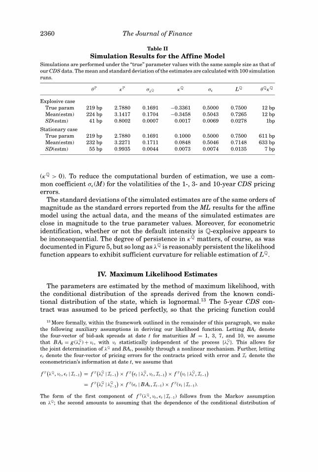
2360 The Journal of Finance
Table IISimulation Results for the Affine Model
Simulations are performed under the “true” parameter values with the same sample size as that ofour CDS data. The mean and standard deviation of the estimates are calculated with 100 simulationruns.
θP κP σλQ κQ σε LQ θQκQ
Explosive caseTrue param 219 bp 2.7880 0.1691 −0.3361 0.5000 0.7500 12 bpMean(estm) 224 bp 3.1417 0.1704 −0.3458 0.5043 0.7265 12 bpSD(estm) 41 bp 0.8002 0.0007 0.0017 0.0069 0.0278 1bp
Stationary caseTrue param 219 bp 2.7880 0.1691 0.1000 0.5000 0.7500 611 bpMean(estm) 232 bp 3.2271 0.1711 0.0848 0.5046 0.7148 633 bpSD(estm) 55 bp 0.9935 0.0044 0.0073 0.0074 0.0135 7 bp
(κQ > 0). To reduce the computational burden of estimation, we use a com-mon coefficient σε(M) for the volatilities of the 1-, 3- and 10-year CDS pricingerrors.
The standard deviations of the simulated estimates are of the same orders ofmagnitude as the standard errors reported from the ML results for the affinemodel using the actual data, and the means of the simulated estimates areclose in magnitude to the true parameter values. Moreover, for econometricidentification, whether or not the default intensity is Q-explosive appears tobe inconsequential. The degree of persistence in κQ matters, of course, as wasdocumented in Figure 5, but so long as λQ is reasonably persistent the likelihoodfunction appears to exhibit sufficient curvature for reliable estimation of LQ.
IV. Maximum Likelihood Estimates
The parameters are estimated by the method of maximum likelihood, withthe conditional distribution of the spreads derived from the known condi-tional distribution of the state, which is lognormal.13 The 5-year CDS con-tract was assumed to be priced perfectly, so that the pricing function could
13 More formally, within the framework outlined in the remainder of this paragraph, we makethe following auxiliary assumptions in deriving our likelihood function. Letting BAt denotethe four-vector of bid-ask spreads at date t for maturities M = 1, 3, 7, and 10, we assumethat BAt = g (λQ
t ) + νt , with νt statistically independent of the process {λQt }. This allows for
the joint determination of λQ and BAt, possibly through a nonlinear mechanism. Further, lettingεt denote the four-vector of pricing errors for the contracts priced with error and It denote theeconometrician’s information at date t, we assume that
f P(λQ, νt , εt | It−1
) = f P(λ
Qt | It−1
) × f P(εt | λQ
t , νt , It−1
) × f P(νt | λQ
t , It−1
)= f P
(λ
Qt | λQ
t−1
) × f P(εt | BAt , It−1) × f P(νt | It−1).
The form of the first component of f P(λQ, νt , εt | It−1) follows from the Markov assumptionon λQ; the second amounts to assuming that the dependence of the conditional distribution of

Default and Recovery Implicit in Term Structure of Sovereign CDS 2361
be inverted for λQ.14 The 1-, 2-, 3-, and 10-year contracts are assumed to bepriced with normally distributed errors with mean zero and standard devia-tions σε(M)|Bidt(M) − Askt(M)|, where the σε(M) are constants depending onthe maturity of the contract, M. Time-varying variances that depend on thebid-ask spread allow for the possibility that the fits of our one-factor modelsdeteriorate during periods of market turmoil when bid-ask spreads widen sub-stantially. Conveniently, σε(M) measures the degree of mispricing by the modelrelative to bid-ask spreads.
The risk-free interest rate (term structure) is assumed to be constant. Weexperiment with using a two-factor affine model (an A1(2) model in the nomen-clature of Dai and Singleton (2000)) for rt, but we obtain virtually identicalresults to those with a constant riskfree rate.15 A simple arbitrage argument(see, e.g., Duffie and Singleton (2003)) shows that CDS spreads are approxi-mately equal to the spreads on comparable maturity, par floating rate bondsfrom the same issuer as the reference bonds underlying the CDS contract. Theprices of these bonds are not highly sensitive to the level of interest rates andthis underlies the insensitivity of our findings to the introduction of a stochasticriskfree rate.
A. ML Estimates of One-Factor Models
The ML estimates of the parameters (expressed on an annual time scale) andtheir associated standard errors are presented in Table III. Across all threecountries, and regardless of whether LQ is a fixed or free parameter, there is astriking contrast between the parameters governing the Q- and P-dynamics ofλQ. Indeed, in the cases of Mexico (constrained or unconstrained) and Turkey(unconstrained), the point estimates for κQ are negative, implying that thedefault intensity λQ is explosive under Q; whereas κP > 0 so λQ is P-stationaryfor all three countries. These large differences between the Q and P distributionsare indicative of substantial market risk premiums related to uncertainty aboutfuture arrival rates of credit events.
From these parameter estimates, we can back out the coefficients for the mar-ket prices of risk, δ0 and δ1, as defined in equation (5). The values for (Mexico,Turkey, Korea) are δ0 = (−7.36, −2.29, −6.16) and δ1 = (−1.35, −0.48, −0.98)
εt on λQt and νt can be summarized by BAt, which itself is fully determined by λ
Qt and νt; and
the third follows from the independence assumption underlying our assumed decomposition ofBAt. Finally, the assumptions that f P(νt | It−1) does not depend on the parameters governingf P(λQ
t | λQ
t−1) and f P(εt | BAt , It−1), and that the Mth element of f P(εt | BAt , It−1) is the density of aN(0, σ 2
ε (M)(Bidt(M) − Askt(M))2) imply our likelihood function.14 The 5-year contract was chosen because of its relative liquidity. The liquidities of the 5-year
contracts are enhanced, for all three countries examined, by their inclusion in the Dow JonesCDX.EM traded index of emerging market CDS spreads.
15 For checking the sensitivity of our results to the presence of stochastic interest rates we onceagain shifted to an affine model for reasons of computational tractability. Within the affine settingwe can allow for stochastic interest rates that are correlated with λQ and still obtain closed-formsolutions for survival probabilities and zero-coupon bond prices.
2362 The Journal of Finance
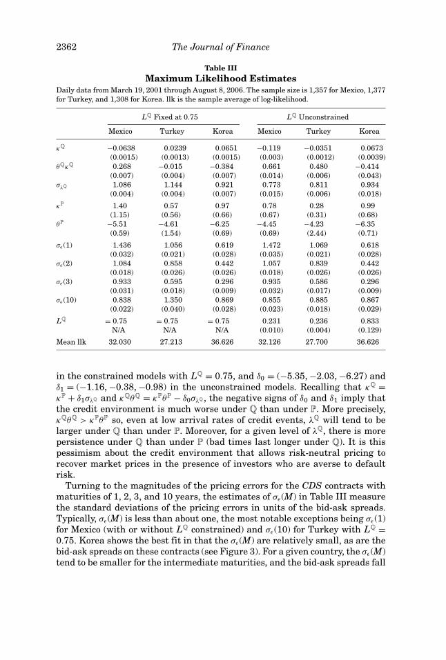
Table IIIMaximum Likelihood Estimates
Daily data from March 19, 2001 through August 8, 2006. The sample size is 1,357 for Mexico, 1,377for Turkey, and 1,308 for Korea. llk is the sample average of log-likelihood.
LQ Fixed at 0.75 LQ Unconstrained
Mexico Turkey Korea Mexico Turkey Korea
κQ −0.0638 0.0239 0.0651 −0.119 −0.0351 0.0673(0.0015) (0.0013) (0.0015) (0.003) (0.0012) (0.0039)
θQκQ 0.268 −0.015 −0.384 0.661 0.480 −0.414(0.007) (0.004) (0.007) (0.014) (0.006) (0.043)
σλQ 1.086 1.144 0.921 0.773 0.811 0.934(0.004) (0.004) (0.007) (0.015) (0.006) (0.018)
κP 1.40 0.57 0.97 0.78 0.28 0.99(1.15) (0.56) (0.66) (0.67) (0.31) (0.68)
θP −5.51 −4.61 −6.25 −4.45 −4.23 −6.35(0.59) (1.54) (0.69) (0.69) (2.44) (0.71)
σε (1) 1.436 1.056 0.619 1.472 1.069 0.618(0.032) (0.021) (0.028) (0.035) (0.021) (0.028)
σε (2) 1.084 0.858 0.442 1.057 0.839 0.442(0.018) (0.026) (0.026) (0.018) (0.026) (0.026)
σε (3) 0.933 0.595 0.296 0.935 0.586 0.296(0.031) (0.018) (0.009) (0.032) (0.017) (0.009)
σε (10) 0.838 1.350 0.869 0.855 0.885 0.867(0.022) (0.040) (0.028) (0.023) (0.018) (0.029)
LQ = 0.75 = 0.75 = 0.75 0.231 0.236 0.833N/A N/A N/A (0.010) (0.004) (0.129)
Mean llk 32.030 27.213 36.626 32.126 27.700 36.626
in the constrained models with LQ = 0.75, and δ0 = (−5.35, −2.03, −6.27) andδ1 = (−1.16, −0.38, −0.98) in the unconstrained models. Recalling that κQ =κP + δ1σλQ and κQθQ = κPθP − δ0σλQ , the negative signs of δ0 and δ1 imply thatthe credit environment is much worse under Q than under P. More precisely,κQθQ > κPθP so, even at low arrival rates of credit events, λQ will tend to belarger under Q than under P. Moreover, for a given level of λQ, there is morepersistence under Q than under P (bad times last longer under Q). It is thispessimism about the credit environment that allows risk-neutral pricing torecover market prices in the presence of investors who are averse to defaultrisk.
Turning to the magnitudes of the pricing errors for the CDS contracts withmaturities of 1, 2, 3, and 10 years, the estimates of σε(M) in Table III measurethe standard deviations of the pricing errors in units of the bid-ask spreads.Typically, σε(M) is less than about one, the most notable exceptions being σε(1)for Mexico (with or without LQ constrained) and σε(10) for Turkey with LQ =0.75. Korea shows the best fit in that the σε(M) are relatively small, as are thebid-ask spreads on these contracts (see Figure 3). For a given country, the σε(M)tend to be smaller for the intermediate maturities, and the bid-ask spreads fall

Default and Recovery Implicit in Term Structure of Sovereign CDS 2363
(on average, as seen from Table I) with increasing maturity, so our models tendto fit somewhat better for M = 2 and 3 than for M = 1 or 10.
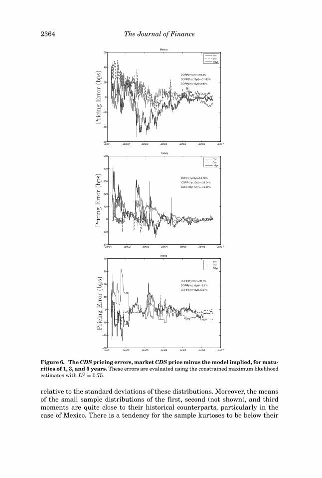
The time-series of CDS pricing errors, measured by the market minus themodel-implied spreads and evaluated at the parameters with LQ = 0.75, areplotted in Figure 6. The high degree of co-movement in the CDS spreads acrossmaturities and countries is much less evident in the corresponding pricing er-rors. In the cases of Mexico and Turkey, the pricing errors on the 1- and 10-yearcontracts are negatively correlated, suggesting that there is some tension infitting both of these spreads simultaneously. For Korea, on the other hand, ourone-factor model appears to price the short-dated contracts equally well in thatCorr(ε(1), ε(3)) = 0.89. The pricing errors on long-dated Korean contracts movein a largely uncorrelated way with those at the short end. A more indepth anal-ysis of these pricing errors and the potential role of a second factor is exploredin Section IV.B. At this juncture we simply highlight the small magnitudes ofthe standard deviations of these errors, typically less than one bid-ask spread.
There are several notable differences between the maximum likelihood esti-mates of the models with and without LQ fixed. Perhaps most striking is thefact that the unconstrained estimates of LQ for Mexico and Turkey are ap-proximately 0.23, much smaller than the market convention of 0.75. Standardlikelihood ratio statistics reject the constraint LQ = 0.75 at conventional sig-nificance levels. On the other hand, for Korea the estimate is quite close to themarket convention. Accompanying the relatively small values of LQ for Mexicoand Turkey are relatively larger values of κQθQ and smaller values of both κQ
and κP (compared to their counterparts in the models with LQ = 0.75). Thelarger values of κQθQ are intuitive: To match spreads with a lower loss rate, the“intercept” of the λQ process under the Q distribution must be larger.16
The relatively larger value of the log-likelihood function in the unconstrainedmodel is attributable to the component associated with the dynamic propertiesof λQ under P, and not to the component associated with the pricing errors.Accordingly, to gain further insight into the relative goodness-of-fits of theconstrained and unconstrained models, we examine the model-implied small-sample distributions of various moments of the CDS spreads and their firstdifferences (time changes). Ten-thousand time series, each of length 1,500 (theapproximate length of our samples), are simulated and the means and standarddeviations of the small-sample distributions of various moments are computed.Among the moments examined are the mean, standard deviation, skewness,and kurtosis, and the autocorrelations of the levels of CDS spreads and theslope of the CDS curve.
Table IV displays the means and standard deviations of the small-sampledistributions of mean, skewness, and kurtosis for Mexico and Turkey, alongwith their sample counterparts. For the first through fourth central moments,the differences between the means of the small-sample distributions across thecorresponding models with and without LQ constrained are small, certainly
16 Conditional on λQt , λ
Q
t+1 will tend to be larger in the model with the lower estimate of LQ. SinceκQ < 0 in the unconstrained models for Mexico and Turkey, λQ does not have a finite Q-mean.
2364 The Journal of Finance
Jan01 Jan02 Jan03 Jan04 Jan05 Jan06 Jan07
0
20
40
60Mexico
CORR(1yr,3yr)=18.2%
CORR(3yr,10yr)=2.97%
1yr3yr10yr
Prici
ng
Err
or(b
ps)
Jan01 Jan02 Jan03 Jan04 Jan05 Jan06 Jan07
0
100
200
300
400
500Turkey
CORR(1yr,3yr)=51.86%
1yr3yr10yr
Prici
ng
Err
or(b
ps)
Jan01 Jan02 Jan03 Jan04 Jan05 Jan06 Jan07
0
10
20
30
40Korea
CORR(1yr,3yr)=89.1%
CORR(1yr,10yr)=12.7%
CORR(3yr,10yr)=5.69%
1yr3yr10yr
Prici
ng
Err
or(b
ps)
Figure 6. The CDS pricing errors, market CDS price minus the model implied, for matu-rities of 1, 3, and 5 years. These errors are evaluated using the constrained maximum likelihoodestimates with LQ = 0.75.
relative to the standard deviations of these distributions. Moreover, the meansof the small sample distributions of the first, second (not shown), and thirdmoments are quite close to their historical counterparts, particularly in thecase of Mexico. There is a tendency for the sample kurtoses to be below their

Default and Recovery Implicit in Term Structure of Sovereign CDS 2365
Table IVThe Small-Sample Moments of CDS Spreads
The small-sample means and standard deviations (in brackets) of the 1-, 5-, and 10-year CDSspreads, along with their sample counterparts, are reported in basis points. MCC refers to MonteCarlo results for the model with LQ = 0.75, and MCU refers to the Monte Carlo results for the mod-els with unconstrained LQ. ACF1 and ACF2 refer to the first- and second-order autocorrelations,respectively, and slope is the 10-minus 1-year spread.
Mexico Turkey
Moment Sample MCC MCU Sample MCC MCU
E[1 yr] 55 59 [18] 57 [21] 355 306 [183] 294 [168]E[5 yr] 166 155 [40] 151 [47] 563 504 [191] 495 [193]E[10 yr] 213 200 [39] 195 [47] 607 520 [152] 531 [175]
Skew[1 yr] 0.95 1.28 [.56] 1.16 [.60] 1.09 1.50 [.69] 1.31 [.73]Skew[5 yr] 0.74 0.94 [.49] 0.84 [.54] 0.51 0.97 [.57] 0.88 [.61]Skew[10 yr] 0.62 0.71 [.45] 0.67 [.50] 0.48 0.89 [.54] 0.92 [.60]
Kurt[1 yr] 2.64 4.86 [2.3] 4.34 [2.2] 3.24 5.53 [3.3] 4.75 [3.0]Kurt[5 yr] 2.65 3.75 [1.6] 3.44 [1.6] 2.10 3.75 [1.8] 3.49 [1.7]Kurt[10 yr] 2.56 3.26 [1.2] 3.11 [1.2] 2.02 3.58 [1.6] 3.60 [1.8]
ACF1(5 yr) 0.996 0.989 [.005] 0.992 [.004] 0.995 0.992 [.004] 0.994 [.003]ACF2(5 yr) 0.991 0.978 [.009] 0.984 [.007] 0.991 0.985 [.007] 0.988 [.006]ACF1(slope) 0.993 0.990 [.004] 0.993 [.003] 0.963 0.985 [.008] 0.991 [.006]ACF2(slope) 0.988 0.981 [.008] 0.986 [.007] 0.940 0.970 [.016] 0.983 [.012]
model-implied small-sample counterparts, but the former are within one stan-dard deviation of the latter.
At first glance, we expected larger differences in the implied autocorrelationsof CDS spreads across the constrained (C) and unconstrained (U) models, be-cause κPC > κPU (see Table III). However our models are parameterized on anannual time scale so, over moderate horizons, the differences in model-implied(first- and second-order) autocorrelations of CDS spreads are small. The model-implied autocorrelations for the slope for Turkey are a bit larger than theirsample counterparts, but otherwise the model and sample autocorrelations arevery similar (Table IV). Of course the higher degree of P persistence with LQ
treated as a free parameter will manifest itself over sufficiently long horizons.However, the effects of κPC > κPU on our analysis of risk premiums in Section Vare negligible at the 1-year horizon. At the 5-year horizon, the differences areagain negligible for Mexico, though they are material for Turkey.
In the light of these findings, how should we set LQ? Consistent with our the-oretical and small-sample analyses in Section III, the choice of LQ does matter.Yet the primary differences across values of LQ as dispersed as 0.23 and 0.75(at least as revealed by the moments we examine) are in the P-persistenceproperties of λQ, and these differences revealed themselves only over quite longhorizons. Additionally, there is the possibility that specification error is com-promising our models’ abilities to fit the highly persistent and volatile nature ofspreads for Mexico and Turkey. Korean spreads are equally persistent, but theyare smaller and less volatile, and it seems plausible that our lognormal model

2366 The Journal of Finance
Table VOLS Regressions of CDS Spreads on Principal Components
For each country, PC1 and PC2 are the first and second principal components of the respectivecountry’s term structure of CDS spreads. β̂ is the estimated loading and R2 is the coefficient ofdetermination for the regression.
Mexico Turkey Korea
PC1 PC2 PC1 PC2 PC1 PC2
Mat. β̂ R2 β̂ R2 β̂ R2 β̂ R2 β̂ R2 β̂ R2
1 yr 0.22 89.8% 0.59 8.4% 0.46 97.2% 0.78 2.8% 0.35 95.4% 0.56 4.3%2 yr 0.38 97.5% 0.49 2.1% 0.47 99.8% 0.13 0.1% 0.40 98.2% 0.39 1.7%3 yr 0.47 99.3% 0.25 0.4% 0.46 99.8% −0.16 0.1% 0.43 99.5% 0.19 0.4%5 yr 0.54 99.4% −0.31 0.4% 0.43 99.1% −0.40 0.8% 0.48 99.8% −0.10 0.1%
10 yr 0.54 98.6% −0.50 1.1% 0.40 98.6% −0.44 1.2% 0.55 97.1% −0.70 2.8%
is a somewhat better approximation for these spreads. Given that our resultsfor Korea are supportive of market convention and that most of our subsequentanalysis is (qualitatively) robust to the choice of LQ, we henceforth focus on thecase of LQ = 0.75.
B. Is One Factor Enough?
Up to this point we have chosen to focus on a single-factor model for λQ, largelybecause, for a given sovereign, the first PC of the CDS spreads explains a verylarge percentage of the variation for all maturities. However, the precedingdiscussion of pricing errors in one-factor models leads us naturally to inquireabout the dimensions along which an additional factor might improve the fit ofour model, if at all.
Table V displays the factor loadings and the percentage variation explainedfrom projections of the CDS spreads onto the first two PCs of the data.17 Asnoted at the outset of our analysis, PC1 explains a large percentage of thevariation in spreads for all countries and all maturities. Indeed, for maturitiesof 3 years and longer, PC1 accounts for at least 97% of the variation in allof the spreads. Moreover, parallel to the findings for the term-structures ofthe U.S. Treasury or swap markets (Litterman and Scheinkman (1991)), thefirst PC emerges as a “level” factor, as reflected in the roughly constant factorloadings across maturities (for a given sovereign). As expected, our one-factormodel with default intensity λQ picks up this level factor: Regressing the timeseries of model-implied λQ onto PC1 yields an R2 of 99.0% for Mexico, 98.6% forTurkey, and 98.7% for Korea.
As an additional, more demanding check on the fit of our models, we displayin Table VI the correlations between the CDS spreads and the slopes of the
17 This PC analysis was conducted using the covariance matrix of the levels of spreads.

Default and Recovery Implicit in Term Structure of Sovereign CDS 2367
Table VIThe Small-Sample Moments of the CDS Slope
The CDS slope measures the difference between the 10-year and the 1-year CDS spreads, in basispoints. Both the sample moments and the small-sample moments (MC) are reported. For the lattercase, 10,000 time series, each of length 1,500, were simulated and the sample moments for eachseries were computed. The top panel reports moments relating to the level of the slope, and thebottom panel reports moments relating to the change in the slope. Standard deviations of thesmall-sample distributions are given in brackets.
Korea Mexico Turkey
S = 10 yr − 1 yr Sample MC Sample MC Sample MC
E[S] 34 46 [5] 158 141 [21] 229 214 [45]Corr(S, 1 yr) 0.60 0.87 [.12] 0.77 0.96 [.02] −0.60 −0.33 [.57]Corr(S, 2 yr) 0.67 0.88 [.11] 0.87 0.96 [.02] −0.48 −0.30 [.57]Corr(S, 3 yr) 0.72 0.88 [.11] 0.90 0.97 [.02] −0.43 −0.27 [.58]Corr(S, 5 yr) 0.77 0.90 [.11] 0.95 0.98 [.01] −0.37 −0.23 [.60]Corr(S, 10 yr) 0.85 0.93 [.10] 0.96 0.99 [.01] −0.35 −0.21 [.61]
Korea Mexico Turkey
Sample MC Sample MC Sample MC
Corr(� S,� 1 yr) −0.36 0.58 [.26] −0.04 0.88 [.08] −0.77 −0.63 [.35]Corr(� S,� 2 yr) −0.09 0.60 [.26] 0.40 0.89 [.07] −0.58 −0.58 [.36]Corr(� S,� 3 yr) −0.005 0.62 [.25] 0.52 0.90 [.06] −0.50 −0.53 [.38]Corr(� S,� 5 yr) 0.11 0.67 [.24] 0.67 0.94 [.05] −0.39 −0.47 [.41]Corr(� S,� 10 yr) 0.33 0.74 [.22] 0.80 0.97 [.04] −0.16 −0.44 [.43]
CDS curves, using levels and first differences, for the historical sample and asimplied by our models.18 Though the patterns in these correlations are quitedifferent across countries (most notably the different signs for Turkey versusKorea and Mexico), our one-factor models match the correlations of levels ofCDS spreads and slopes quite closely. The models do less well at matching thecorrelations among the first differences of these variables, though this is to beexpected as first differences are essentially daily innovations in these variables.Even for changes, the match is quite good for Turkey at all maturities and forMexico and Korea at the longer maturities.
Among the various maturities, the one-factor model misprices the 1-year con-tract most severely. As we have just seen, our models are also challenged bythe low degree of correlation between innovations in the 1-year CDS spreadsand the slopes of the CDS curves. Taken together, these observations suggestthat there are components of the short ends of the CDS curves that are not wellcaptured by our one-factor models. Further support for this assessment comesfrom regressing, for each country, the 1-year pricing error on the second PC ofthe CDS spreads, which gives R2s of 67.6% for Mexico, 45.9% for Turkey, and65.1% for Korea. The corresponding R2s for the pricing errors on longer matu-rity contracts decline substantially with maturity in the cases of Mexico and
18 The first row of Table VI confirms that our models do a reasonable job of matching the averageslopes of the CDS curves for our sample period.

2368 The Journal of Finance
Table VIIOLS Regressions of CDS Bid/Ask Spreads on the First Two Principal
Components of Bid/Ask Spreads
Mexico Turkey
PC1 PC2 PC1 PC2
Mat. β̂ R2 β̂ R2 β̂ R2 β̂ R2
1 yr 0.44 89.7% −0.79 8.2% 0.57 93.7% 0.65 4.9%2 yr 0.47 93.2% −0.18 0.4% 0.48 95.2% 0.17 0.5%3 yr 0.44 93.8% 0.18 0.4% 0.45 94.6% −0.25 1.1%5 yr 0.44 95.6% 0.37 1.9% 0.37 92.8% −0.38 4.0%10 yr 0.45 93.9% 0.42 2.3% 0.33 81.6% −0.59 10.4%
Turkey, suggesting that what PC2 is picking up is primarily a short-maturityphenomenon in these markets.
Based on conversations with traders, it seems that the most likely explana-tion for this “anomalous” behavior of the 1-year contract is due to a liquidityor supply/demand premium. We are told that large institutional money man-agement firms often use the short-dated CDS contract as a primary tradingvehicle for expressing views on sovereign bonds. The sizable trades involvedin these transactions introduce an idiosyncratic “liquidity” factor into the be-havior of the 1-year contract. Consistent with this view, the bid-ask spreads asa percentage of the underlying CDS spreads are notably larger for the 1-yearcontract.
Of interest then is whether or not there is a component of the bid-ask spreadsthat is orthogonal to the first PC of spreads, that is, whether there are largeidiosyncratic components of the bid-ask spreads for specific maturities.19 Thisquestion is answered in Table VII where we report the results from regressingthe bid-ask spreads of the individual CDS contracts onto the first two principalcomponents of the bid-ask spreads for Mexico and Turkey. There is a smallrole for a second factor in the bid-ask spreads, concentrated almost entirely atthe 1- and 10-year maturity points. These patterns suggest that there mightindeed be something special about the 1- and possibly 10-year contracts from aliquidity perspective. The roles of such illiquidity or trading pressures on CDSspreads are issues that we hope to explore in future research.
V. On Priced Risks in Sovereign CDS Markets
The large differences between the parameters governing λQ under the risk-neutral and the actual measures suggest that there is a systematic risk relatedto changes in future arrival rates of sovereign credit events that is priced in
19 The bid-ask spreads are highly correlated with the corresponding levels of spreads. In par-ticular, the correlations between PC1 of the CDS spreads (contract prices) and PC1 of the bid-askspreads are 80.7% for Mexico and 86.3% for Turkey.

Default and Recovery Implicit in Term Structure of Sovereign CDS 2369
the CDS market. To examine the economic underpinnings of the priced risks inthe sovereign CDS markets, we take the ML estimates obtained in Section IVand construct two measures of fitted CDS spreads. The first is the actual fittedspread CDSt(M) from (1). The second is
CDSPt (M ) =
2(1 − RQ)∫ t+M
tEP
t
[λQ
u e− ∫ ut (rs+λQ
s ) ds]
du
2M∑j=1
EPt
[e− ∫ t+.5 j
t (rs+λQs ) ds
] , (10)
obtained from (1) by replacing all of the expectations EQ with expectationsunder the physical measure P, EP. If market participants are neutral towardsthe risk of variation over time in λQ, then CDSP
t (M ) should replicate the corre-sponding market price CDSt(M). Put differently, a mark-up in the CDS spreadrelative to the pseudo-spread implies that the buyer of the CDS contract is will-ing to pay a premium for holding the CDS contract, while the seller demands apremium. This is similar to what is found in equity options markets where thetime-variation of volatility is a priced risk. To quantify the role of risk premiumsregarding variation in λQ, in percentage terms, we report20
CRPt(M ) ≡ (CDSt(M ) − CDSP
t (M ))/
CDSPt (M ). (11)
The percentage contribution of the risk premiums to spreads at the 1-yearmaturity (CRPt(1)) are displayed in Figure 7. The correlations between theCRPs are 93.6% for (Mexico, Turkey), 89.6% for (Mexico, Korea), and 88.0%for (Turkey, Korea). This high degree of co-movement in the CRPs is strikinggiven the very different credit qualities and geo-political features of the threecountries examined. Risk premiums induced more volatility in the spreads dur-ing the early part of our sample, with the gap between CDSt and CDSP
t (on apercentage basis) being most volatile for Mexico. During the later period ofour sample, when spreads in the credit markets were tight and when talks of“reaching for yield” were prevalent, the CRPs (as seen through our lognormalmodel) turned negative. Figure 8 shows that CRPt(M) tends to increase withmaturity.21 Evidently, not only does risk increase with horizon, but its effecton premiums increases on a percentage basis as the maturity of the contractincreases. Additionally, unlike in the case of the 1-year contract, the CRPs donot become negative at the long end of the maturity spectrum.
To assist in interpreting the various “peaks” in the contributions of risk pre-miums to spreads during our sample period, in Figure 8 we mark the dates ofseveral key economic events around the times of these peaks. The early partof our sample was dominated by economic and political events in South Amer-ica. Argentina faced an economic crisis in the spring of 2001 and President de
20 We stress that neither CDSt nor CDSPt involve the physical intensity λP. As emphasized by
Jarrow, Lando, and Yu (2005) and Yu (2002), this information cannot be extracted from bond orCDS spread data alone.
21 This measure of the effects of premiums on spreads is larger still when M = 10.

2370 The Journal of Finance
Jan01 Jan02 Jan03 Jan04 Jan05 Jan06 Jan07
0
20
40
60
80
100
120
140
CORR(MEX,TUR)=93.63%
CORR(MEX,KOR)=89.58%
CORR(TUR,KOR)=87.95%
MexicoTurkeyKorea
CRP
≡(C
DS−CDS
P)�CDS
P(%
)
Figure 7. The percentage difference between the 1-year CDS price and the 1-yearpseudo-CDS for Mexico, Turkey and Korea.
la Rua removed his Minister of Economics and introduced a fiscal austerityprogram. This was followed in the summer of 2001 by a “zero-deficit” plan inan attempt to avoid major bank runs and reverse the depletion of foreign re-serves (Zhang (2003)). A year later, in the summer of 2002, the prospect of theleft-wing candidate Lula Da Silva winning the presidential elections in Brazilroiled sovereign debt markets. He subsequently won the election in October ofthat year. Perhaps not surprisingly, all of these political developments in SouthAmerica had much larger effects on the risk premiums for Mexico than on thosefor Turkey or Korea.
The simultaneous and large jumps both in CDS spreads and the CRPs duringMay 2004 have their roots in investors’ portfolio reallocations due to macroeco-nomic developments in the U.S. During the second quarter of 2004 there was asubstantial increase in nonfarm payrolls in the United States. This, combinedwith comments by representatives of the Federal Reserve, led market partici-pants to expect a tightening of monetary policy. A reason that these concernshad large and widespread effects on spreads is that both financial institutionsand hedge funds had substantial positions in “carry trades.” They were borrow-ing short-term in dollars and investing in long-term bonds, often high-yield andemerging market bonds issued in various currencies. The unexpected strength

Default and Recovery Implicit in Term Structure of Sovereign CDS 2371
Jan01 Jan02 Jan03 Jan04 Jan05 Jan06 Jan070
100
200
300
400
500
600
700
P)/CDSP (%)
MexicoTurkeyKorea
Sept 11
Lula Election
Lula Elected
Unwinding ofCarry Trades dueto Concerns onU.S. MonetaryPolicy Tightening
GM & FordDowngradedto Junk
Unwinding ofCarry Trades
Argentina Crisis
Figure 8. CRP(5) ≡ (CDS− CDSP)/CDSP for Mexico, Turkey, and Korea, computed usingthe 5-year CDS contract.
in the U.S. economy led to an unwinding of some of these trades and, conse-quently, an across-the-board adjustment in spreads on corporate and sovereigncredits.22 This episode illustrates the importance of changes in investors’ ap-petite for exposure to credit, as a global risk class, for co-movements in yields.The induced changes in yields on the sovereign credits examined here (ap-parently) had nothing directly to do with the inherent credit qualities of theissuers.
In March of 2005 there were similarly sized run-ups in CRPt(5) associatedwith the deteriorating credit quality of General Motors and Ford in the U.S.In the middle of March Fitch downgraded GM, S&P changed its rating out-look to negative, and Moody’s placed GM on review for a downgrade. Thesechanges were followed with similarly negative outlooks on Ford in early April2005. Concurrently, there was a substantial widening of spreads not only onthe individual-name CDS contracts for these issuers, but also on high-yield
22 These concerns were widely noted in the media at the time. “In a single day, May 7, yieldson Brazilian bonds jumped 1.52 percentage points as the unexpectedly strong jobs report in theU.S. increased the likelihood of higher short-term rates. (Henry (2004))” See also the discussion inCogan (2005).

2372 The Journal of Finance
corporate indices (e.g., Packer and Wooldridge (2005)). Figure 8 shows that theretrenchment in high-yield positions extended to emerging markets as well.
Finally, CRP(5) shows a sizable increase during the late spring of 2006. Onceagain the evidence supports an increased aversion to exposure to emergingmarket credit risk rather than reassessments of the fundamental economicstrengths of individual countries. There was a broad sell-off in emerging mar-ket equities and a concurrent correction in foreign currency markets as hedgefunds and other leveraged investors unwound carry trades in the emergingmarket currencies (e.g., IMF (2006)). During this episode Turkey in particularexperienced large balance of payments pressures on its currency, as well asdomestic political uncertainties related to its EU accession.
An interesting feature of the time-series of CRP(5)s in Figure 8 is that adjust-ments to Mexico’s risk premiums had the largest percentage effects on spreadsthroughout most of our sample period. During the first half of our sample thisis no doubt attributable to the political and economic upheavals in Latin Amer-ica. The gaps between the countries’ CRP(5) are smaller during the second halfof our sample, and the events in early 2006 had the largest effect on Turkey.As noted, this was most likely a manifestation of domestic policy and politicalissues in Turkey at the time.
Another striking country-specific episode in Figure 8 is the brief, but large,run-up in CRP(5) for Korea in the early part of 2003. This was a period of risingdelinquencies on credit card debts following a very rapid expansion in consumerborrowing. Concurrently, the financial stability of several credit card companiesand investment trusts was called into question (Kang (2004)). In addition, theconglomerate SK Global reported material accounting irregularities in March,2003 and this contributed to existing concerns about the stability of the Koreanfinancial system (Cooper and Madigan (2003)).
Comparison of Figures 3 and 8 suggests that episodes in which the risk pre-miums associated with variation in λQ were large (as measured by CRP) werealso episodes in which the bid-ask spreads on the CDS contracts were large.23
This is true of Mexico to some degree and, on an absolute basis, it is particu-larly true of Turkey over the early part of our sample. However, other than for abrief period in early 2002 for Mexico, the changes in bid-ask spreads for Mexicoand Korea were much smaller and their ratios (ask − bid)/bid remained below10%. Thus, although the gradual increase in the liquidity of the sovereign CDSmarkets during our sample period no doubt contributed to the downward trendin spreads, changes in liquidity do not appear to have been a major source ofvariation in the CRPt(M).
The strengths of the economies in all three of the countries examined depend,to varying degrees and through various economic channels, on the strength of
23 Concurrent movements in liquidity and credit quality are often observed in credit markets. Asshown by Duffie and Singleton (1999), the pricing formulas we use can be adapted to accommodateliquidity risk by adjusting the discount rate from rt + λ
Qt to rt + λ
Qt + �t , where �t is a measure of
liquidity costs. Longstaff et al. (2005) use this extended framework in their analysis of corporatebond and CDS contracts. They assume that �t = 0 in their pricing of corporate CDS contracts or,equivalently, that CDS spreads are driven nearly entirely by variation in λQ.

Default and Recovery Implicit in Term Structure of Sovereign CDS 2373
30
35
40
45
50
55
60
65
70
75
Mar-01 Mar-02 Mar-03 Mar-04 Mar-05 Mar-06
ISM
Ind
ex
-15
-10
-5
0
5
10
15
20
25
Y o
n Y
IP G
row
th
ISM + 3 months
Korea
Mexico
Turkey
Figure 9. The year-on-year growth rates of industrial production in Korea, Turkey, andMexico (right-hand scale), and the ISM Index of U.S. Manufacturing led 3 months (left-hand scale).
the U.S. economy. This is apparent from Figure 9, which displays the year-on-year growth rates of industrial production (right scale) and the Institutefor Supply Management (ISM) index of U.S. manufacturing shifted one quar-ter ahead (left scale).24 The sample correlations of ISM and the growth rates(one quarter hence) for Korea, Turkey, and Mexico are 0.66, 0.65, and 0.58,respectively. For Korea, the most persistent gap between these measures ofeconomic growth occurred during 2004 when Korea experienced a marked slow-down in private consumption expenditures in part as a consequence of theconsumer debt overhang from 2003 noted above. Turkey shows much morecountry-specific variation in growth, though one can visually see the secularco-movement with the U.S. economy.
With these observations about the economic events associated with peaks inthe CRPs in mind, we turn next to a more in-depth exploration of the rela-tionships between CRPt(M) and various measures of global risk and financialmarket developments. Figure 10 displays the (standardized) CBOE VIX volatil-ity index and the spread between the U.S. Industrial 10-year BB Yield and the
24 The data on industrial production were obtained from the International Monetary Fund. TheISM index of manufacturing, based on a monthly survey of purchasing and supply executivesthroughout the U.S., is constructed by weighting seasonally adjusted new orders, production, em-ployment, supplier deliveries and inventories.

2374 The Journal of Finance
Jan01 Jan02 Jan03 Jan04 Jan05 Jan06 Jan07
0
1
2
3
4
CORR(PC1,VIX) = 90.79%
CORR(PC1,US) = 85.37%
CORR(VIX,US) = 74.99%
PC1 of CRP(5)VIX IndexUS Spread
Figure 10. The CBOE VIX index, the spread between the U.S. BB corporate yield the6-month Treasury bill rate (U.S.-Spread), and the first principal component of CRP(5) =(CDS(5) − CDSP(5))/CDSP(5), for Mexico, Turkey, and Korea. All variables are demeaned andscaled by their respective sample standard deviations.
6-month Treasury bill yield (U.S.-Spread)25 plotted against the first principalcomponent (CRP-PC1) of the CRPt(5) for Mexico, Turkey, and Korea. We viewVIX, a widely watched measure of event risk in credit markets, as a central in-gredient in investors’ appetite for exposure to the high-yield bond credit class.The view that a significant component of the recent declines in VIX is due tochanging investors’ appetite for risk is widely expressed in the financial press(see, e.g., “Drop in volatility measure ‘reflects investors growing appetite forrisk,’ Dennis (2006)).” More formally, for the overlapping portions of our sam-ples, the risk premium component of VIX computed by Todorov (2006) (seehis Figure 5) appear to track our standardized VIX series in Figure 10 quiteclosely.
We view the positive correlation between CRP and U.S.-Spread as havingat least two economic sources. First, we have seen from our discussion of Fig-ure 8 that the unwinding of carry trades had large effects on sovereign CDSspreads, especially during 2004 and 2006. The “long long-dated corporate, short
25 The yield data were downloaded from Bloomberg Financial Services.

Default and Recovery Implicit in Term Structure of Sovereign CDS 2375
short-dated Treasury” exposure captured by U.S.-Spread should reflect changesin risk or liquidity premiums associated with the desirability of carry-tradepositions. While we do not have direct measures of the interest rate or de-fault risk premiums underlying movements in U.S.-Spread, we highlight twocomplementary studies that suggest that changes in these premia were im-portant during our sample period. Berndt et al. (2004) show that, within theirlognormal framework, a majority of the variation in corporate CDS spreadsbetween the summer of 2002 and the end of 2004 was due to variation indefault risk premiums and not expected loss rates on these bonds. For theU.S. Treasury markets, Cochrane and Piazzesi (2006) find that the seem-ingly anomalous behavior of yields on long-term U.S. Treasury bonds in recentyears is largely explained by declining risk premiums and not by changes inexpectations about future yields. U.S.-Spread reflects, in addition, the slopeof the U.S. Treasury yield curve, which is widely watched as an indicatorof the stance of U.S. monetary policy and, thus, of the condition of the U.S.economy.
The co-movement of CRP-PC1 with VIX in Figure 10 is notable; their samplecorrelation is over 90%. A strong correlation between VIX volatility and U.S.corporate credit spreads has been extensively documented (see, e.g., Collin-Dufresne, Goldstein, and Spencer Martin (2001) and Schaefer and Strebulaev(2004)). That VIX, a domestic equity volatility index, is also highly correlatedwith spreads on sovereign entities as widely dispersed as Mexico and Turkeysupports the view that VIX is a key factor in investors’ appetite for global“event risk” in credit markets. Turning to U.S.-Spread, the association withCRP-PC1 is relatively weak over the first half of our sample. However, par-ticularly during the run-up in CRP(5)s in the springs of 2004 and 2006, U.S.-Spread and CRP-PC1 track each other closely. This appears to be a graphicaldepiction of the effects on risk premiums of the widespread unwinding of carrytrades.
More formally, we next examine the relative contributions to the variationin the individual country CRP(5)s of the risk factors VIX, U.S.-Spread, and theown-country implied currency option volatility (CVOL). The risk factor CVOLis included to assist in capturing the effects of capital flows induced both byexternal macroeconomic developments and their effects on the flows of goodsand capital, and the effects of local political and economic events on the creditqualities of sovereign issuers. Table VIII displays the regression estimates withNewey–West t-statistics reported in squared brackets, for our entire sampleperiod and the second half of our sample.26 Focusing first on the univariateregressions over the entire sample period, VIX has the most explanatory powerfor CRP(5) for Mexico, U.S.-Spread for Turkey, and CVOL has slightly moreexplanatory power than U.S.-Spread for Korea. In the multivariate regressionsfor Mexico and Turkey both VIX and U.S.-Spread have significant explanatory
26 Reliable data for Turkey on the implied volatilities of currency options was available only forthe second half of our sample and this explained the partial results for Turkey in the upper half ofTable VIII. Fifty lags were used in computing the Newey–West standard errors.
2376 The Journal of Finance
Tab
leV
III
OL
SR
egre
ssio
ns
ofth
e5-
year
Ris
kP
rem
ium
,M
easu
red
by(C
DS
−C
DS
P)/
CD
SP,o
nth
eC
BO
EV
IXIn
dex,
the
U.S
.In
dust
rial
10-y
ear
BB
Yie
ldM
inu
sth
e6-
mon
thT
reas
ury
,an
dth
e6-
mon
thC
urr
ency
Impl
ied
Vol
atil
ity,
CV
OL
,for
the
Res
pect
ive
Cou
ntr
ies
Mex
ico
(200
1/4/
24–2
006/
8/10
)T
urk
ey(2
001/
3/19
–200
6/8/
9)K
orea
(200
1/3/
19–2
006/
8/8)
U.S
.R
-sqr
U.S
.R
-sqr
U.S
.R
-sqr
VIX
Spr
ead
CV
OL
(%)
VIX
Spr
ead
CV
OL
(%)
VIX
Spr
ead
CV
OL
(%)
22.8
486
.04
9.20
68.6
610
.50
52.6
5[1
9.06
][9
.54]
[4.7
3]78
.75
75.1
340
.92
76.9
146
.17
57.0
8[8
.80]
[15.
27]
[9.7
6]80
.73
61.2
755
.29
59.7
8[7
.44]
[9.8
7]15
.69
34.5
092
.04
4.38
27.2
283
.84
5.25
29.5
262
.84
[10.
27]
[8.1
4][4
.44]
[6.4
8][1
.75]
[3.5
2]16
.63
36.6
8−7
.18
92.1
82.
3224
.02
35.1
379
.32
[11.
81]
[10.
19]
[−1.
54]
[1.1
6][4
.90]
[5.3
7]
Mex
ico
(200
3/12
/12–
2006
/8/1
0)T
urk
ey(2
003/
12/1
2–20
06/8
/9)
Kor
ea(2
003/
12/1
2–20
06/8
/8)
U.S
.R
-sqr
U.S
.R
-sqr
U.S
.R
-sqr
VIX
Spr
ead
CV
OL
(%)
VIX
Spr
ead
CV
OL
(%)
VIX
Spr
ead
CV
OL
(%)
17.9
537
.50
14.4
439
.73
12.2
729
.66
[3.8
9][3
.64]
[2.7
3]46
.30
76.4
936
.67
76.5
737
.15
81.1
0[8
.80]
[7.5
1][1
2.37
]30
.89
24.9
011
.46
68.0
631
.86
43.6
8[2
.92]
[5.7
3][3
.49]
5.04
41.1
478
.50
5.60
31.3
980
.96
1.22
35.9
081
.30
[2.5
9][8
.34]
[3.3
5][7
.39]
[0.7
4][1
2.69
]5.
8842
.07
−3.8
178
.71
0.45
24.7
36.
3490
.59
1.23
34.8
21.
7381
.36
[3.1
7][7
.93]
[−0.
57]
[0.3
9][9
.14]
[10.
77]
[0.7
4][7
.02]
[0.3
0]

Default and Recovery Implicit in Term Structure of Sovereign CDS 2377
power. In the case of Korea, U.S.-Spread and CVOL contribute explanatorypower, while VIX is statistically insignificant.
While the reduced-form nature of our regressions introduces some ambiguityinto the interpretation of these regressions, the evidence is consistent with theview that much of the effect of risk premiums on CDS spreads for Mexico wasassociated with investors’ appetite for exposure to event risk. At least over theearly part of our sample, there is notable co-movement between VIX, the CRPs,and major political/economic events throughout Latin America. The incremen-tal explanatory power from U.S.-Spread for Mexico is, at least partially, owing toinvestors’ reallocations of capital through the unwinding of carry trades. Thatthese “price pressure” effects of capital flows mattered for Mexico is furthersupported by the results for the second half of our sample during which U.S.-Spread had by far the most explanatory power for CRP(5) (see the lower halfof Table VIII). The correlation between U.S.-Spread and CRP(5) may also re-flect real economic risk associated with the close trading relationship betweenMexico and the U.S. Notably, after accounting for VIX and U.S.-Spread, the coef-ficient on CVOL is statistically insignificant, both for the entire and the secondhalf of our sample period. This suggests that the currency option volatilitiesin Carr and Wu’s (2006) analysis of Mexican CDS spreads may have served asstand-ins for the more fundamental macroeconomic and event risks embodiedin VIX and U.S.-Spread.
Turning to the results for Turkey, over the entire sample period for which weonly have data on VIX and U.S.-Spread, these two risk factors had comparableexplanatory power, suggesting that many of the considerations discussed forMexico were relevant for Turkey as well. Over the second half of our sample,for which we have data on all three risk factors, once again U.S.-Spread is akey explanatory variable for variation in CRP(5). However, unlike for Mexico,CVOL has significant explanatory power and the coefficient on VIX is statisti-cally insignificant. The economic underpinnings of the substantial incrementalexplanatory power of CVOL for Turkey were the large current account deficitsand substantial portfolio inflows during the latter half of our sample. Turkeyexperienced a consumption-led expansion that was partly financed by theselarge portfolio inflows. Many foreign investors hedged the currency risk of theirlocal bond positions so it seems natural that the placement and subsequent un-winding of carry trades induced a significant correlation between CVOL andCRP(5).
The results for Korea show that all three risk factors had significant explana-tory power for CRP(5) for the entire sample period. Interestingly, the contribu-tion of VIX is muted, certainly relative to the case of Mexico, and, like Turkey,the coefficient on VIX is statistically insignificant for the second half of oursample. We have been told by some investment bankers that investors in Ko-rean bonds have a more “local” focus and that, consequently, spreads are not ashighly correlated with VIX as for some other countries. Comparing our resultsfor all three countries, it may simply be that, at least recently, VIX has servedmore as a measure of risk in the U.S. (or perhaps regionally in the Americas).The explanatory power of U.S.-Spread and CVOL for Korea are surely in part a

2378 The Journal of Finance
reflection of the dependence of Asian economies, through exports and imports,on the strength of the U.S. economy (see Figure 9).
VI. On the Sensitivity of Results to Modeling Choices
All of our model-based findings on the structure of risk premiums in sovereignmarkets are premised on our having adopted a plausible model for λQ, and onour results being largely robust to alternative specifications of f P(ε | BAt , It−1),the conditional density of the pricing errors (see footnote 13).
For the purpose of valuing CDS contracts, the literature has typically as-sumed either that λQ follows a square-root diffusion (e.g., the Zhang (2003)analysis of Argentinean CDS spreads and the Longstaff et al. (2005) analysisof U.S. corporate CDS spreads) or that ln(λQ) follows an Ornstein-Uhlenbeck(Gaussian) process (e.g., the Berndt et al. (2004) analysis of U.S. corporate CDSspreads). We explored in-depth the relative goodness of fits of these two mod-els, as well as a model in which λQ follows a “three-halves” diffusion (see Ahnand Gao (1999) for a discussion of this model in a term structure setting), andconcluded that, for the sovereign CDS spreads and sample period examined,the lognormal model fit the best.
More concretely, as is illustrated in Figure 11 for the case of Mexico withLQ = 0.75, the magnitudes of the pricing errors tend to be ordered, with thoseof the lognormal model lying between those of the three-halves and affine(square-root) models. The differences between the pricing errors are relativelylarge during relatively volatile periods as might be expected given their dif-ferent specifications of the conditional variances of λQ.27 For example, during2002 when risk premiums in Mexican markets were historically large (Figure8), the errors for the lognormal model were closest to zero, with those of theaffine (three-halves) model being notably positive (negative). That is, the affine(three-halves) model gives CDS spreads that are too low (high). The orderingof mispricing is reversed at the 10-year maturity, with the affine model fit-ting somewhat better than the lognormal model during 2002. All three modelsfit comparably well during the low-volatility period in 2003. Comparisons likethese, along with the additional information provided in an earlier draft of thispaper (that is available from the authors’ web sites) led us to favor, on bal-ance, the lognormal model for this study. Berndt (2006) formally assesses thegoodness-of-fit of similar models for corporate default using the specificationtest proposed by Hong and Li (2005) and also concludes that the lognormalmodel provides a better fit than affine models.
As is evident in Figures 6 and 11, the pricing errors from all three mod-els exhibit positive autocorrelation. The likelihood functions underlying theparameter estimates used to compute these pricing errors presumed thatthey are serially independent (see footnote 13). Given the relatively smallvariances of the pricing errors compared to the variances of the fitted CDS
27 The instantaneous standard deviations of λQ depend on the square-root, level, and three-halvespower in the affine, lognormal, and three-halves models, respectively.
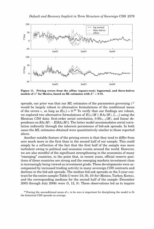
Default and Recovery Implicit in Term Structure of Sovereign CDS 2379
Jan02 Jan03 Jan04-50
0
50
1003
Yea
r
Jan02 Jan03 Jan04-50
0
50
100
10 Y
ear
log normal
affinethree halves
Figure 11. Pricing errors from the affine (square-root), lognormal, and three-halvesmodels of λQ for Mexico, based on ML estimates with LQ = 0.75.
spreads, our prior was that our ML estimates of the parameters governing λQ
would be largely robust to alternative formulations of the conditional meanof the errors ε, so long as E[εt] = 0.28 To verify that our findings are robust,we explored two alternative formulations of E[εt(M ) | BAt(M ), It−1] using theMexican CDS data: first-order serial correlation, 0.95εt−1(M), and linear de-pendence on BAt(M) − E[BAt(M)]. The latter model accommodates serial corre-lation indirectly through the inherent persistence of bid-ask spreads. In bothcases the ML estimates obtained were quantitatively similar to those reportedabove.
Another notable feature of the pricing errors is that they tend to differ fromzero much more in the first than in the second half of our sample. This couldsimply be a reflection of the fact that the first half of the sample was moreturbulent owing to political and economic events around the world. However,we are also mindful of the significant strengthening in the economies of many“emerging” countries, to the point that, in recent years, official reserve posi-tions of these countries are strong and the emerging markets investment classis increasingly being viewed as investment grade. These developments were ac-companied by increased trading activity in many sovereign CDS contracts anddeclines in the bid-ask spreads. The median bid-ask spreads on the 5-year con-tract for the entire sample (Table I) were (10, 30, 10) for (Mexico, Turkey, Korea),and the corresponding medians for the second half of the sample (December2003 through July 2006) were (5, 12, 8). These observations led us to inquire
28 Forcing the unconditional mean of εt to be zero is important for disciplining the model to fitthe historical CDS spreads on average.

2380 The Journal of Finance
Table IXMaximum Likelihood Estimates for the Second Half of the Sample
Daily data from November 26, 2003 through August 8, 2006. The sample size is 679 for Mexico and699 for Turkey. llk is the sample average of log-likelihood.
LQ Fixed at 0.75 LQ Unconstrained
Mexico Turkey Mexico Turkey
κQ −0.035 −2.83e-006 −0.0339 −0.0365(0.0043) (0.0021) (0.0091) (0.0044)
θQκQ 0.132 0.0722 0.12 0.391(0.02) (0.0088) (0.082) (0.032)
σλQ 1.10 1.18 1.11 0.972(0.0087) (0.0059) (0.046) (0.027)
κP 5.13 2.21 5.19 1.60(2.5) (1.8) (2.6) (1.3)
θP −5.87 −4.94 −5.91 −4.25(0.21) (0.51) (0.34) (0.55)
σε (1) 0.954 0.802 0.954 0.835(0.038) (0.029) (0.038) (0.033)
σε (3) 0.778 0.862 0.778 0.86(0.027) (0.048) (0.027) (0.047)
σε (7) 0.722 0.663 0.722 0.674(0.038) (0.037) (0.039) (0.038)
σε (10) 1.09 0.995 1.08 0.95(0.065) (0.039) (0.064) (0.034)
LQ 0.75 0.75 0.781 0.367N/A N/A (0.18) (0.029)
Mean llk 31.497 27.358 31.497 27.419
whether the parameter estimates—and, in particular, the characterizations ofthe credit-event arrival and recovery processes—are different when the modelis fit to the second half of our sample.29
Focusing first on Mexico, the point estimates of σλQ (Table IX) are comparableto those in Table III based on the entire sample period. However, both κQ andκQθQ are closer to zero for the second half of the sample, implying that λQ isless explosive and, risk-neutrally, the mean arrival rate of a credit event issmaller at small values of λQ. Notably, this (risk-neutrally) improved creditenvironment during the second half of our sample is being traded off againsta much larger value of LQ: The unconstrained estimate of LQ is 0.78, which isvery close to the value set by traders in marking their sovereign CDS books(though with a standard error of 0.18).30 Although the relative contributions of
29 We focus on Mexico and Turkey, because these are the cases where the unconstrained MLestimates of LQ were low relative to the values set by most traders. As with most split-sampleanalyses, examination of the second half of a sample sheds light on parameter drift due to changesin economic regimes, but it comes with the potential cost of using a sample that is not representativeof the data generating process.
30 To assure ourselves that this result was not due to our choice of starting values we consideredfive random seeds for LQ drawn from the Uniform [0.1,0.9] distribution and optimized the likelihood

Default and Recovery Implicit in Term Structure of Sovereign CDS 2381
event arrival and recovery have changed, the risk premiums associated withunpredictable variation in λQ remain large. In fact, with unconstrained LQ, themodel-implied estimate of δ1, the slope coefficient on λQ in our specification ofmarket prices of risk, is −1.16 over the entire sample and −4.71 over the secondhalf of the sample.31
Our findings for Turkey are closer to those obtained over the entire sam-ple period. There is a moderate decline in κQθQ, with κQ remaining largelyunchanged. Accompanying the lower value of κQθQ is a larger value of LQ, anincrease from 0.24 to 0.37. The overall fit, as measured by the smaller estimatedσε(M) (and smaller bid-ask spreads) for several maturities, also improves overthe second half of the sample. This is perhaps to be expected given that thissubsample was a relatively less turbulent time.
Within our limited sample of three countries, it is intriguing that the es-timates of LQ are larger for the more highly rated countries. That is, for thehigher rated countries, our likelihood function calls for relatively favorable risk-neutral processes for the arrival rates of credit events, balanced against largervalues of LQ. Analogous to the relatively larger jump-at-default risk premiumsfor more highly rated corporate bonds (see, e.g., Huang and Huang (2003) andBerndt et al. (2004)), it is plausible that (risk-neutral) loss rates are indeedmuch larger for highly rated countries like Korea or Mexico. The economic cir-cumstances that would bring either of these countries to restructure its externaldebt would surely have hugely adverse consequences globally, relative to eventsthat would bring, say, Turkey to restructure. As the market for recovery swapson sovereign debts develops, it will be interesting to compare our findings tothe market’s ordering of LQ, as reflected in the values of these contracts.
VII. Concluding Remarks
We have documented systematic, priced risks associated with unpredictablefuture variation in the credit-event arrival intensity λQ for three countries:Mexico, Turkey, and Korea. The effects of these risk premiums on CDS spreadsco-vary strongly across countries, and large moves in these premiums have nat-ural interpretations in terms of political, macroeconomic, and financial marketdevelopments during our sample period. Most notably, our results suggest that,during some subperiods, a substantial portion of the co-movement among theterm structures of sovereign spreads across countries was induced by changes ininvestors’ appetites for credit exposure at a global level, rather than by reassess-ments of the fundamental strengths of these specific sovereign economies. Thatis, our findings support the view that there is a global high-yield credit class andthat spreads in all markets are affected simultaneously as both the financingcosts of “risk arbitrage” positions change and investors’ attitudes towards bear-ing the risks of these positions change over time. Spillovers of real economic
function for all five seeds. The seed giving the largest value of the likelihood function was thenpursued to a higher degree of accuracy. For the estimates reported in Table IX, the starting valuesfor LQ ranged between 0.78 and 0.47.
31 Recall that our model is parameterized at annual intervals, so the implications of these esti-mates of δ1 for moderate time horizons are not hugely different.

2382 The Journal of Finance
growth in the U.S. to economic growth in other regions of the world also con-tribute to the co-movements among the risk premiums in the sovereign marketsexamined.
Country-specific and regional economic risks were also present and reflectedin our models’ estimates. This was particularly the case with Turkey, thoughsuch specific risks were also present for Mexico during the early part of oursample, and for Korea during 2003 to 2004. Even in the presence of these spe-cific risks, our one-factor lognormal models do quite a good job of capturingthe variation over time in the entire term structure of CDS spreads (matu-rities ranging from 1 to 10 years). Further examination of the pricing errorsrevealed that the 1-year contracts were the least well priced by our one-factormodels. Both anecdotal evidence from conversations with CDS traders and theco-movements of these errors with bid-ask spreads suggest that liquidity orthe effects of supply/demand pressures on prices might underlie this localizedmispricing.
Finally we argued, using both analytic calculations of the scores of the like-lihood functions and Monte Carlo analysis of small-sample distributions, thatthe parameters governing the conditional distribution of the arrival rate ofcredit events (λQ) and the loss given an event (LQ) are separately identifi-able using time-series data on the term structure of CDS spreads. In practice,the model-implied distributions of λQ were indeed different as LQ was variedover the admissible parameter space, confirming that times-series informationon the term structure of CDS spreads is informative about loss rates. However,the unconstrained maximum likelihood estimates of LQ for our full sample pe-riod were in the region of the market convention, LQ = 0.75, only in the case ofKorea.
This left open the question of whether or not there are features of the distri-bution of CDS spreads for countries like Mexico or Turkey that our lognormalmodels are not capturing and that, once captured, would give rise to estimatesfor LQ closer to market convention. We took a small step toward exploring thispossibility by re-estimating our models for these countries over the second halfof our sample period, a less turbulent period with smaller bid-ask spreads. Theestimate of LQ for Mexico over this subsample was very close to the value of0.75 set by traders, while for Turkey it was larger than in the full sample, butstill less than 0.50.
Looking ahead, further insights into the default and recovery processes forsovereign issuers may also be revealed by a joint analysis of CDS spreadsand other credit-sensitive derivative products. The expanding offerings of op-tions on CDS contracts and various basket or index products offers hope inthis direction.32 Even when additional sources of market information aboutsovereign credit are readily available, our analysis suggests that it will be useful
32 In this spirit, though in the context of credit risk for corporate issuers, Das and Hanouna(2006) and Le (2006) achieve the separate identification of the parameters governing LQ and λQ
by combining models for pricing CDS contracts with models for pricing the issuer’s (firm’s) equity,under the assumption that equity is a “zero-recovery” instrument. Both of these studies rely on aparametric functional dependence of λQ on observable state variables, however.

Default and Recovery Implicit in Term Structure of Sovereign CDS 2383
to incorporate the rich information embodied in the term structure of CDSspreads.
REFERENCESAhn, Dong-Hyun, and Bin Gao, 1999, A parametric nonlinear model of term structure dynamics,
Review of Financial Studies 12, 721–762.Altman, Edward, Brooks Brady, Andrea Resti, and Andrea Sironi, 2003, The link between default
and recovery rates: Theory, empirical evidence and implications, Working paper, Stern Schoolof Business New York University.
Berndt, Antje, 2006, Specification analysis of reduced-form credit risk models, Working paper,Tepper School, Carnegie Mellon University.
Berndt, Antje, Rohan Douglas, Darrell Duffie, Mark Ferguson, and David Schranzk, 2004, Measur-ing default risk premia from default swap rates and EDFs, Working paper, Stanford University.
Carr, Peter, and Liuren Wu, 2007, Theory and evidence on the dynamic interactions betweensovereign credit default swaps and currency options, Journal of Banking and Finance 31,2383–2403.
Cochrane, John, and Monika Piazzesi, 2006, Decomposing the yield curve, Working paper, Univer-sity of Chicago.
Cogan, Philip, 2005, If they all rush for the exit at the same time. . ., Financial Times May 27, 1–2.Collin-Dufresne, Pierre, Robert S. Goldstein, and J. Spencer Martin, 2001, The determinants of
credit spread changes, Journal of Finance 56, 2177–2208.Cooper, James, and Kathleen Madigan, April 7 2003, South Korea: Suddenly impediments to
growth, Working paper, Business Week.Dai, Qiang, and Kenneth Singleton, 2000, Specification analysis of affine term structure models,
Journal of Finance 55, 1943–1978.Das, Sanjiv R., and Paul Hanouna, 2006, Implied recovery, Working paper, Santa Clara University.Dennis, Neil, 2006, Drop in volatility measure “reflects investors growing appetite for risk”, Fi-
nancial Times, November 22, 28.Duffie, Darrell, 1998, Defaultable term structure models with fractional recovery of par, Working
paper, Graduate School of Business, Stanford University.Duffie, Darrell, Lasse Pedersen, and Kenneth Singleton, 2003, Modeling credit spreads on sovereign
debt: A case study of Russian bonds, Journal of Finance 55, 119–159.Duffie, Darrell, and Kenneth Singleton, 1999, Modeling term structures of defaultable bonds, Re-
view of Financial Studies 12, 687–720.Duffie, Darrell, and Kenneth Singleton, 2003, Credit Risk (Princeton University Press, Princeton).Economist, 2004, Argentina’s default, shooting the messenger, September 25, 91.Henry, David, 2004, Ahead of a Fed move, a cash cow runs dry, Business Week, May 24, 1–2.Hong, Yongmiao, and Haitao Li, 2005, Nonparametric specification testing for continuous-time
models with applications to term structure of interest rates, Review of Financial Studies 18,37–84.
Houweling, Patick, and Ton Vorst, 2005, Pricing default swaps: Empirical evidence, Journal ofInternational Money and Finance 24, 1200–1225.
Huang, Jingzhi, and Ming Huang, 2003, How much of the corporate-treasury yield spread is dueto credit risk? A new calibration approach, Working paper, Pennsylvania State University.
Hull, John, Mirela Predescu, and Alan White, 2004, The relationship between credit default swapspreads, bond yields, and credit rating announcements, Working paper, University of Toronto.
IMF, September 2006, Global financial stability report, Working paper, Capital Markets Division,International Monetary Fund.
Jarrow, Robert A., David Lando, and Fan Yu, 2005, Default risk and diversification: Theory andempirical implications, Mathematical Finance 15, 1–26.
Kang, Kenneth H., 2004, Korea: Economic outlook and reforms for 2004, IMF Securities Quarterly,February.
Lando, David, 1998, On Cox processes and credit risky securities, Review of Derivatives Research2, 99–120.

2384 The Journal of Finance
Le, Anh, 2006, Separating the components of default risk: A derivative-based approach, Workingpaper, Stern School, New York University.
Litterman, Robert, and Jose Scheinkman, 1991, Common factors affecting bond returns, Journalof Fixed Income 1, 54–61.
Longstaff, Francis A., Sanjay Mithal, and Eric Neis, 2005, Corporate yield spreads: Default riskor liquidity? New evidence from the credit-default swap market, Journal of Finance 60, 2213–2253.
Moody’s, 2003, Sovereign bond defaults, rating transitions, and recoveries (1985–2002), Workingpaper, Moody’s Investors Service.
Packer, Frank, and Chamaree Suthiphongchai, 2003, Sovereign credit default swaps, BIS QuarterlyReview, December, 81–88.
Packer, Frank, and Philip D. Wooldridge, 2005, Repricing in credit markets, BIS Quarterly Review,June, 1–13.
Schaefer, Stephen M., and Ilya A. Strebulaev, 2004, Structural models of credit risk are useful:Evidence from hedge ratios on corporate bonds, Working paper, Graduate School of Business,Stanford University.
Singh, Manmohan, 2003, Recovery rates from distressed debt—Empirical evidence from chapter11 filings, international litigation, and recent sovereign debt restructurings, Working paper,IMF 03/161.
Todorov, Viktor, 2006, Variance risk premium dynamics, Working paper, Duke University.Xu, D., and C. Wilder, 2003, Emerging market credit derivatives, Working paper, Deutsche Bank.Yu, Fan, 2002, Modeling expected return on defaultable bonds, Journal of Fixed Income 12, 69–81.Zhang, Frank, 2003, What did the credit market expect of Argentina default? Evidence from default
swap data, Working paper, Federal Reserve Board.