Deepika(14 mba5012) transportation ppt

Transportation Problem

By :Deepika Bansal(14MBA5012)

Aim of Transportation Model

To find out optimum transportation schedule keeping in mind cost of transportation to be minimized.

Transportation Problem

Albuquerque(300 unitsrequired)

Des Moines(100 unitscapacity)

Evansville(300 unitscapacity)

Fort Lauderdale(300 unitscapacity)

Cleveland(200 unitsrequired)

Boston(200 unitsrequired)

Figure C.1

What is a Transportation Problem?

• The transportation problem is a special type of LPP where the objective is to minimize the cost of distributing a product from a number of sources or origins to a number of destinations.

• Because of its special structure the usual simplex method is not suitable for solving transportation problems. These problems require special method of solution.

CONT……

• The problem of finding the minimum-cost distribution of a given commodity from a group of supply centers (sources) i=1,…,mto a group of receiving centers (destinations) j=1,…,n

• Each source has a certain supply (si)

• Each destination has a certain demand (dj)• The cost of shipping from a source to a destination is

directly proportional to the number of units shipped

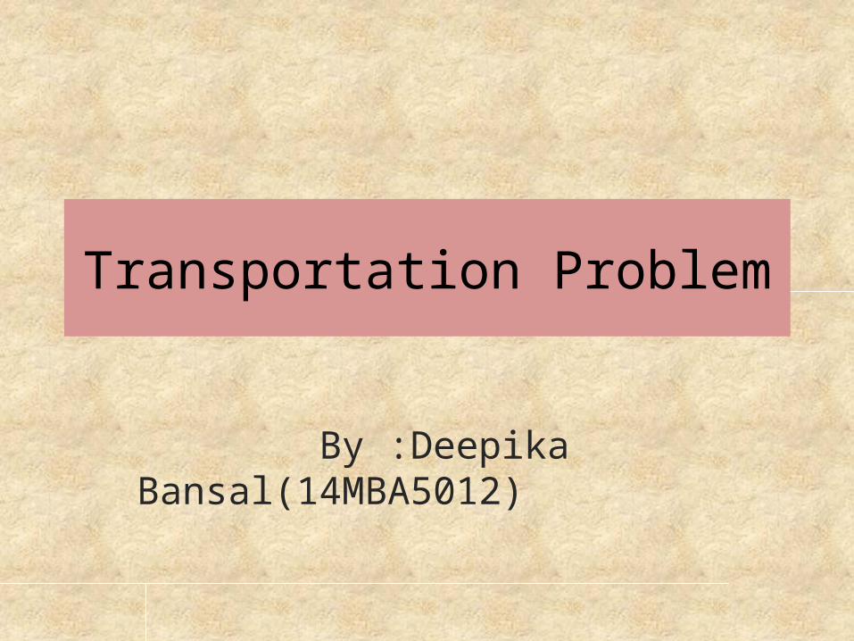
IN SIMPLE LANG……

• “The transportation problem is to transport various amounts of a single homogenous commodity, which are initially stored at various origins , to different destinations in such a way that the total transportation cost is a minimum”.

Assumptions of the Model

• Availability of the quantity.• Transportation of items.• Cost per unit.• Independent cost.• Objective.

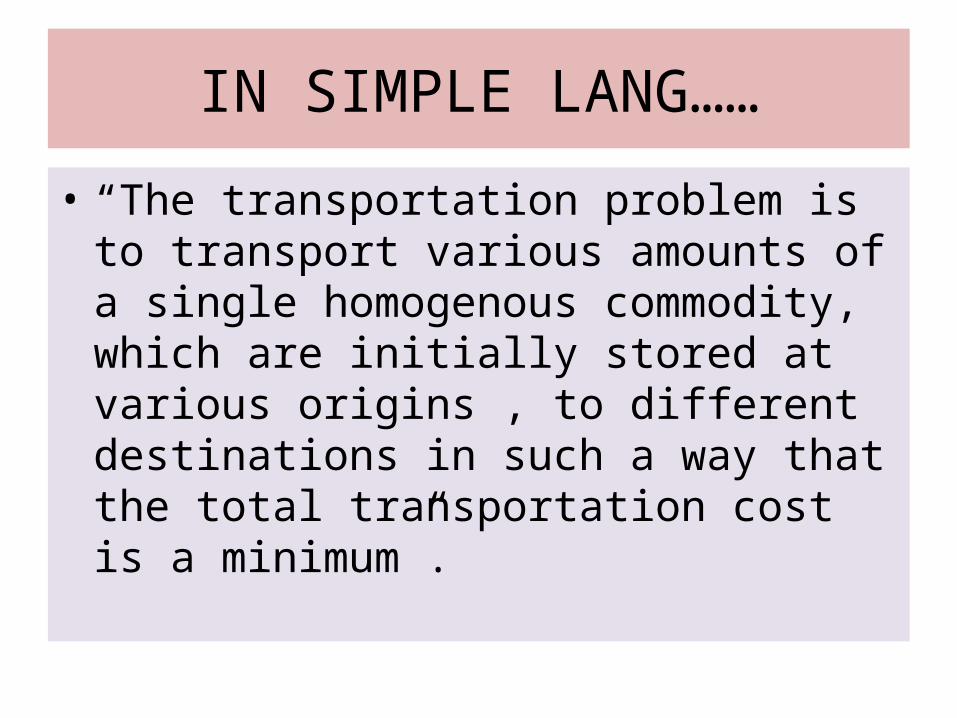
Application of Transportation Problem

Minimize shipping costs

Determine low cost location

Find minimum cost production schedule

TERMINOLOGY USED IN TRANSPORTATIONAL MODEL

Feasible solution: Non negative values of xij where i=1, 2……….m and j=1, 2,…n which satisfy the constraints of supply and demand is called feasible solution.

Basic feasible solution: If the no of positive allocations are (m+n-1). Optimal solution: A feasible solution is said to be optimal solution if it

minimizes the total transportation cost. Balanced transportation problem: A transportation problem in which the total

supply from all sources is equal to the total demand in all the destinations. Unbalanced transportation problem: Problems which are not balanced are

called unbalanced. Matrix terminology: In the matrix, the squares are called cells and form

columns vertically and rows horizontally. Degenerate basic feasible solution: If the no. of allocation in basic feasible

solutions is less than (m+n-1).

Two Types of Transportation Problem

• Balanced Transportation Problem where the total supply equals total demand

• Unbalanced Transportation Problem where the total supply is not equal to the total demand

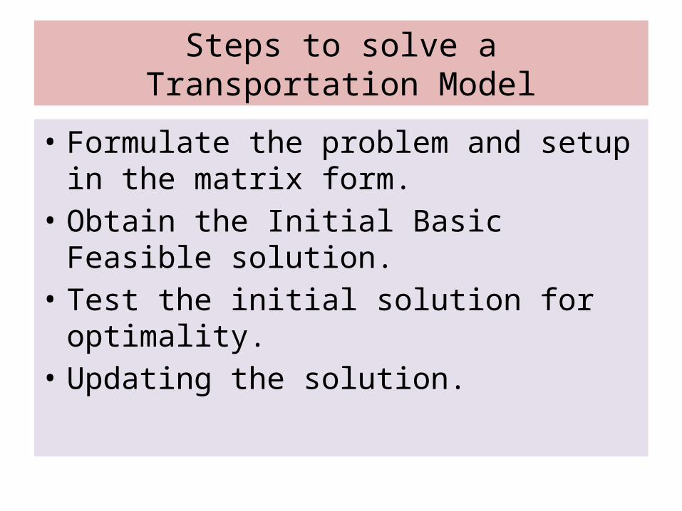
Steps to solve a Transportation Model

• Formulate the problem and setup in the matrix form.

• Obtain the Initial Basic Feasible solution.• Test the initial solution for optimality.• Updating the solution.

GENERAL CONEPTS

ROW

COLUMN

CONT…………

• To solve the transportation problem, it is required that the sum of the supplies at the sources equal the sum of the demands at the destinations. If the total supply is greater than the total demand, a dummy destination is added with demand equal to the excess supply, and shipping costs from all sources are zero. Similarly, if total supply is less than total demand, a dummy source is added.

Phases of Solution of Transportation Problem

• Phase I- obtains the initial basic feasible solution

• Phase II-obtains the optimal basic solution

Initial Basic Feasible Solution

North West Corner Rule (NWCR)

Least Cost Method

Vogle Approximation Method (VAM)

North- West Corner Method (NWCM)

• The simplest of the procedures, used to generate an initial feasible solution is, NWCM. It is so called because we begin with the North West or upper left corner cell of our transportation table.

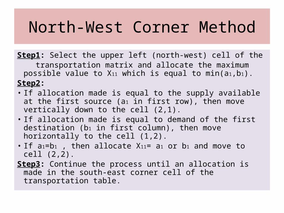
North-West Corner Method

Step1: Select the upper left (north-west) cell of the transportation matrix and allocate the maximum possible

value to X11 which is equal to min(a1,b1).Step2: • If allocation made is equal to the supply available at the

first source (a1 in first row), then move vertically down to the cell (2,1).

• If allocation made is equal to demand of the first destination (b1 in first column), then move horizontally to the cell (1,2).

• If a1=b1 , then allocate X11= a1 or b1 and move to cell (2,2).Step3: Continue the process until an allocation is made in

the south-east corner cell of the transportation table.

Example: Solve the Transportation Table to find Initial Basic Feasible Solution using North-West Corner Method.

Total Cost =19*5+30*2+30*6+40*3+70*4+20*14 = Rs. 1015

Supply19 30 50 10

5 270 30 40 60

6 340 8 70 20

4 14Demand 34

S1

S2

S3

7

9

18

5 8 7 14

D1 D2 D3 D4

Least-Cost Method

• Least-Cost Method consist in allocating as much as possible in the lowest cost cell and then further allocation is done in th cell with second lowest cost cell and so on.

Least-Cost Method

Step1: Select the cell having lowest unit cost in the entire table and allocate the minimum of supply or demand values in that cell.

Step2: Then eliminate the row or column in which supply or demand is exhausted. If both the supply and demand values are same, either of the row or column can be eliminated.

In case, the smallest unit cost is not unique, then select the cell where maximum allocation can be made.

Step3: Repeat the process with next lowest unit cost and continue until the entire available supply at various sources and demand at various destinations is satisfied.

Supply

19 30 50 10

70 30 40 60

40 8 70 20

8Demand 34

S3 18

5 8 7 14

S1 7

S2 9

D1 D2 D3 D4

Supply

19 30 50 10

70 30 40 60

40 8 70 20

8Demand 34

S3 18

5 8 7 14

S1 7

S2 9

D1 D2 D3 D4

Supply

19 50 10

7

70 40 60

40 70 20

Demand 34

D1 D3 D4

7 14

7

9

S1

S2

S3 10

5

Supply

70 40 60

40 70 20

7Demand 34

S2 9

D1 D3 D4

S3 10

5 7 7

Supply

70 40

7

40 70

Demand 34

9

3S3

5 7

S2

D1 D3 Supply

70

2

40

3Demand 345

S2 2

S3 3

D1

• The total transportation cost obtained by this method= 8*8+10*7+20*7+40*7+70*2+40*3= Rs.814Here, we can see that the Least Cost Method involves a lower cost than the North-West Corner Method.

Vogel’s Approximation Method (VAM)

• In this method, each allocation is made on the basis of the opportunity (or penalty or extra) cost that would have been incurred if allocations in certain cells with minimum unit transportation cost were missed. In this method allocations are made so thet the penalty cost is minimized.

Vogel’s Approximation Method (VAM)

Step1: Calculate penalty for each row and column by taking the difference between the two smallest unit costs. This penalty or extra cost has to be paid if one fails to allocate the minimum unit transportation cost.

Step2: Select the row or column with the highest penalty and select the minimum unit cost of that row or column. Then, allocate the minimum of supply or demand values in that cell. If there is a tie, then select the cell where maximum allocation could be made.

Step3: Adjust the supply and demand and eliminate the satisfied row or column. If a row and column are satisfied simultaneously, only of them is eliminated and the other one is assigned a zero value.Any row or column having zero supply or demand, can not be used in calculating future penalties.

Step4: Repeat the process until all the supply sources and demand destinations are satisfied.

Supply Row Diff.

19 30 50 10

70 30 40 60

40 8 70 20

8Demand 34

Col.Diff.

9

10

12

21 22 10 10

D1 D2 D3

S1

S2

S3

5 8 7

D4

14

7

9

18

Supply Row Diff.

19 50 10

5

70 40 60

40 70 20

Demand 34

Col.Diff.

D1 D3 D4

S1 7

S2 9

S3 10

5 7 14

21 10 10

9

20

20

Supply Row Diff.

50 10

40 60

70 20

10Demand 34

Col.Diff. 10 10

40

20

50

D3 D4

S1 2

S2 9

S3 10

7 14

Supply Row Diff.

50 10

2

40 60

Demand 34

Col.Diff.

20

10 50

40

7 4

S1 2

S2 9

D3 D4 Supply Row Diff.

40 60

7 2Demand 34

Col.Diff.

20

7 2

S2 9

D3 D4

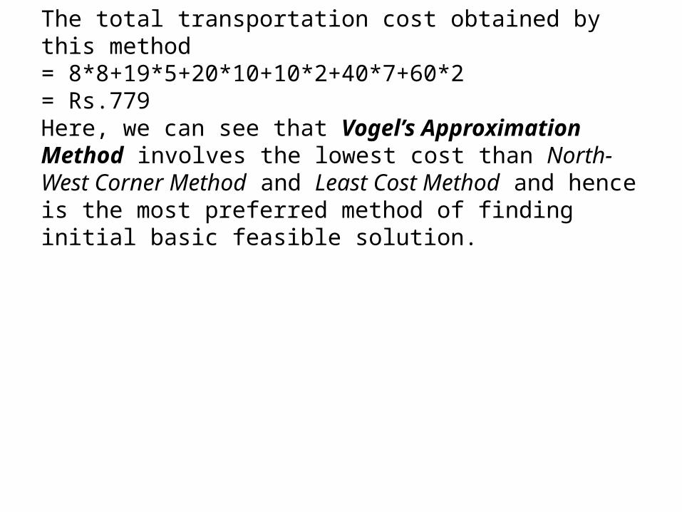
The total transportation cost obtained by this method= 8*8+19*5+20*10+10*2+40*7+60*2= Rs.779Here, we can see that Vogel’s Approximation Method involves the lowest cost than North-West Corner Method and Least Cost Method and hence is the most preferred method of finding initial basic feasible solution.

Optimum Basic Solution

Stepping Stone Method

Modified Distribution Method a.k.a. MODI Method

Optimum Basic Solution:Stepping-Stone Method

1. Select any unused square to evaluate2. Beginning at this square, trace a closed path

back to the original square via squares that are currently being used

3. Beginning with a plus (+) sign at the unused corner, place alternate minus and plus signs at each corner of the path just traced

Stepping-Stone Method

4. Calculate an improvement index by first adding the unit-cost figures found in each square containing a plus sign and subtracting the unit costs in each square containing a minus sign

5. Repeat steps 1 though 4 until you have calculated an improvement index for all unused squares. If all indices are ≥ 0, you have reached an optimal solution.

Problem Illustration

FROMTO A.

ALBUQUERQUE B. BOSTON

C. CLEVELAND

FACTORY CAPACITY

D. DES MOINES 5

4 3100

E. EVANSVILLE 8

4 3300

F. FORT LAUDERDALE

9 7 5300

WAREHOUSE DEMAND 300 200 200 700

Initial Feasible Solution using Northwest Corner Rule

FROMTO A.

ALBUQUERQUE B. BOSTON

C. CLEVELAND

FACTORY CAPACITY

D. DES MOINES 5

4 3100

E. EVANSVILLE 8

4

3 300

F. FORT LAUDERDALE

9 7

5 300

WAREHOUSE DEMAND 300 200 200 700

100

200 100

100 200

IFS= DA + EA +EB + FB + FC = 100(5) + 200(8) + 100(4) + 100(7) + 200(5)= 500 + 1600 + 400 + 700 + 1000 = 4200

$5

$8 $4

$4

+ -

+-

Optimizing Solution using Stepping-Stone Method

To (A)Albuquerque

(B)Boston

(C)Cleveland

(D) Des Moines

(E) Evansville

(F) Fort Lauderdale

Warehouse requirement 300 200 200

Factory capacity

300

300

100

700

$5

$5

$4

$4

$3

$3

$9

$8

$7

From

100

100

100

200

200

+-

-+

1100

201 99

99

100200Figure C.5

Des Moines- Boston index= $4 - $5 + $8 - $4 = +$3


To (A)Albuquerque

(B)Boston

(C)Cleveland

(D) Des Moines

(E) Evansville

(F) Fort Lauderdale


Factory capacity

300

300

100

700

$5

$5

$4

$4

$3

$3

$9

$8

$7

From

100

100

100

200

200

Figure C.6

Start+-

+

-+

-

Des Moines-Cleveland index= $3 - $5 + $8 - $4 + $7 - $5 = +$4

Stepping-Stone MethodTo (A)

Albuquerque(B)

Boston(C)

Cleveland

(D) Des Moines

(E) Evansville

(F) Fort Lauderdale


Factory capacity

300

300

100

700

$5

$5

$4

$4

$3

$3

$9

$8

$7

From

100

100

100

200

200Evansville-Cleveland index= $3 - $4 + $7 - $5 = +$1(Closed path = EC - EB + FB - FC)Fort Lauderdale-Albuquerque index= $9 - $7 + $4 - $8 = -$1(Closed path = FA - FB + EB - EA)


1. If an improvement is possible, choose the route (unused square) with the largest negative improvement index

2. On the closed path for that route, select the smallest number found in the squares containing minus signs

3. Add this number to all squares on the closed path with plus signs and subtract it from all squares with a minus sign


Albuquerque(B)

Boston(C)

Cleveland

(D) Des Moines

(E) Evansville

(F) Fort Lauderdale


Factory capacity

300

300

100

700

$5

$5

$4

$4

$3

$3

$9

$8

$7

From

100

100

100

200

200

Figure C.7

+

+-

-

1. Add 100 units on route FA2. Subtract 100 from routes FB3. Add 100 to route EB4. Subtract 100 from route EA


Albuquerque(B)

Boston(C)

Cleveland

(D) Des Moines

(E) Evansville

(F) Fort Lauderdale


Factory capacity

300

300

100

700

$5

$5

$4

$4

$3

$3

$9

$8

$7

From

100

200

100

100

200

Figure C.8

Total Cost = $5(100) + $8(100) + $4(200) + $9(100) + $5(200)= $4,000

Special Issues in Modeling

Demand not equal to supply Called an unbalanced problem Common situation in the real world Resolved by introducing dummy sources

or dummy destinations as necessary with cost coefficients of zero


Figure C.9

NewDes Moines capacity

To (A)Albuquerque

(B)Boston

(C)Cleveland

(D) Des Moines

(E) Evansville

(F) Fort Lauderdale


Factory capacity

300

300

250

850

$5

$5

$4

$4

$3

$3

$9

$8

$7

From

50200

250

50

150

Dummy

150

0

0

0

150

Total Cost = 250($5) + 50($8) + 200($4) + 50($3) + 150($5) + 150(0)= $3,350


Degeneracy To use the stepping-stone methodology,

the number of occupied squares in any solution must be equal to the number of rows in the table plus the number of columns minus 1

If a solution does not satisfy this rule it is called degenerate

To Customer1

Customer2

Customer3

Warehouse 1

Warehouse 2

Warehouse 3

Customer demand 100 100 100

Warehouse supply

120

80

100

300

$8

$7

$2

$9

$6

$9

$7

$10

$10

From


0 100

100

80

20

Figure C.10

Initial solution is degeneratePlace a zero quantity in an unused square and proceed computing improvement indices

STEPS

1.Construct a transportation table with the given cost of transportation and rim requirement.

2.Determine IBFS.3.For current basic feasible solution check degeneracy

and non-degeneracy. rim requirement=stone square(non-degeneracy) rim requirement != stone square(degeneracy)4.Find occupied matrix.5.Find unoccupied matrix.

Steps (contd…)6.Find opportunity cost of unoccupied cells using

formula: opportunity cost =actual cost-implied cost dij= cij - (ri+kj)7.Unoccupied cell evaluation: (a) if dij>0 then cost of transportation unchanged. (b) if dij=0 then cost of transportation unchanged. (c) if dij<0 then improved solution can be obtain and

go to next step.

STEPS(contd…)

8.Select an unoccupied cell with largest –ve opportunity cost among all unoccupied cell.

9.Construct closed path for the occupied cells determined in step 8.

10.Assign as many as units as possible to the unoccupied cell satisfying rim conditions.

11.Go to step 4 and repeat procedure untilAll dij>=0 i.e reached to the optimal solution.

SPECIAL CASES

• Balanced problem• Unbalanced problem• Non -degeneracy• Degeneracy :occurs in two cases1. Degeneracy occurs in initial basic solution.2. Degeneracy occurs in during the test of optimality.• Profit maximization

.

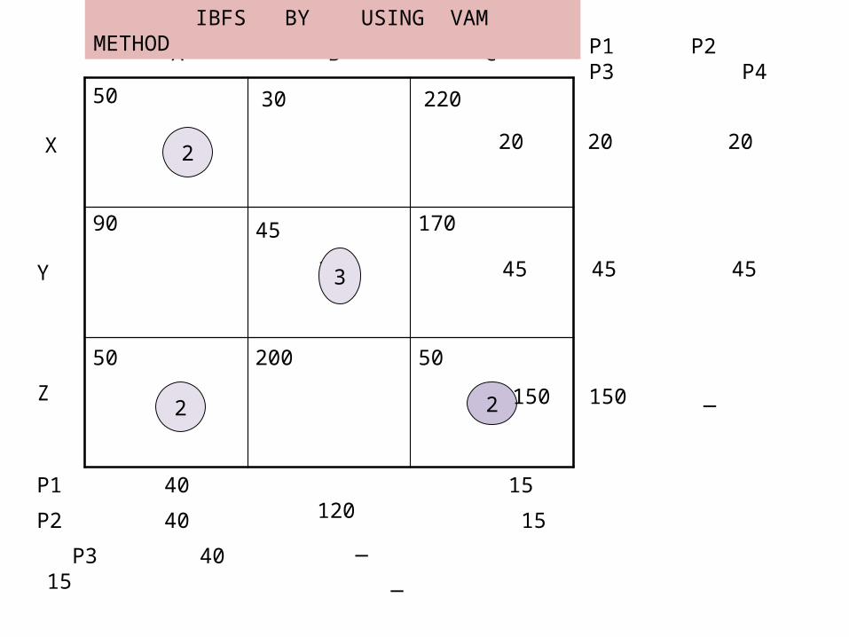
PROBLEM1:Shipping costs are Rs. 10 per kilometer.. What shipping schedule should be used. if the matrix given below the kilometers from source to destination.

destination a b c availability

x 50 30 220 1 y 90 45 170 3 z 50 200 50 4

Requirement 3 3 2 8

A B C

X

Y

Z

30 220

50

90 45 170

50 200 50

30 220

1

2

3

2

2

2 2

3

P1 P2 P3 P4

20 20 20 20

45 45 45 _

150 150 _ _

P1 40 15 120

P2 40 15 _

P3 40 15 _

IBFS BY USING VAM METHOD

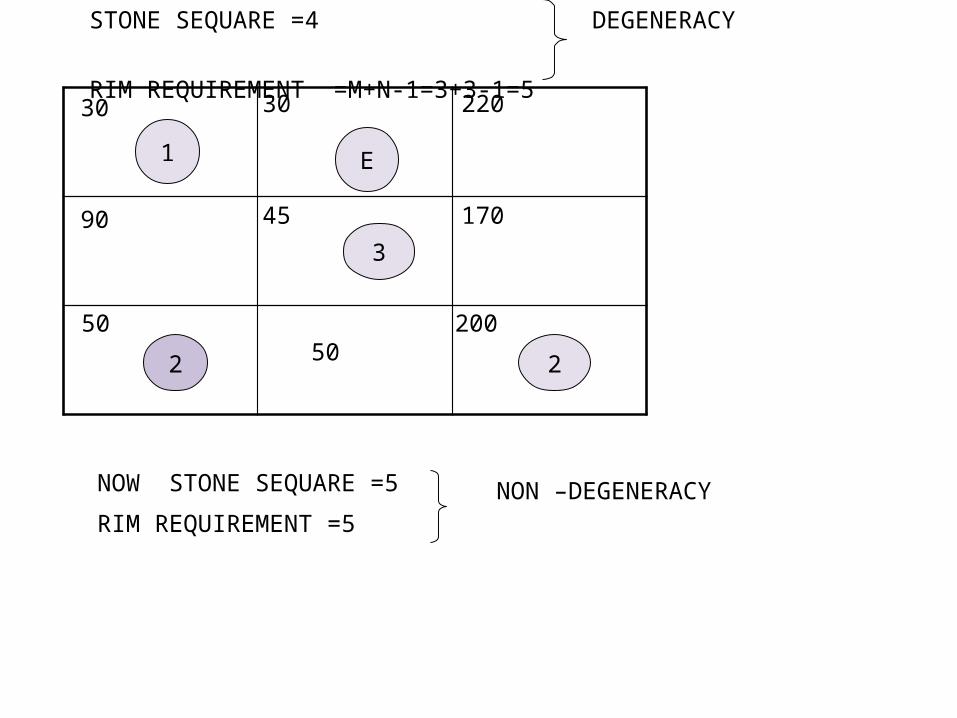
3030 220

90 45 170

50 200 50

1 E

3

2 2

STONE SEQUARE =4

RIM REQUIREMENT =M+N-1=3+3-1=5

DEGENERACY

NOW STONE SEQUARE =5

RIM REQUIREMENT =5NON –DEGENERACY

50 30

45

50 50

50 30 50

0

15

0

OCCUPIED MATRIX UNOCCUPIED MATRIX

10525

170

50

65

30

65

170

OPTIMUL SOLUTION

X A 50*1=50

X B 30*E=_

Y B 45*3=135

Z A 50*2=100

Z C 50*2=100

385 *10=3850

PROBLEM2:DETERMINE THE OPTIMUM SOLUTION FOR THE COMPANY OF TRASPOTATION PROBLEM(USING NWCM AND MODI METHOD)

8 8 15

15 10 17

3 9 10

REQUIREMENT 150 80 50

120

80

80

CAPACITY

F1

F2

F3

W1 W2 W3

WAREHOUSE

FACTORY

W1 W2 W3

F1

F2

F3

8 8 15

15

3

10 17

9 10

120

30 50

30 50

150 80 50

120

80

80

IBFS WITH NWCM


8

15 10

9 10

15 10 11

-7

0

-1

15 10 11

-7

0

-1

5 11

6

-11

3 4

11

14

1588

15 10 17

3 9 10

10

120

30 50

30 50+

+_

_

8

15

3

8 15

10 17

9 10

120 E

80

30 50

STONE SEQUARE=RIM REQUIREMENTDEGENERACY OCCUAR

LOOP CONSTRUCT


8 8

10

3 10

3 3 10 3 3 10

5

7

0

5

7

0

5

6

0

0

15

1710

3

OPTIMUM SOLUTIONF1 W1 8*120 =960

F1 W2 8*E = _

F2 W2 10*80 =800

F3 W1 3*30= 90

F3 W3 10*50 =500

2,350 RS

Deepika(14 mba5012) transportation ppt

Business

Transcript of Deepika(14 mba5012) transportation ppt