DEEP LEARNING TECHNIQUES FOR ANALYZING CLINICAL LUNGCANCER DATA

BY

HAOZE DU

A Thesis Submitted to the Graduate Faculty of

WAKE FOREST UNIVERSITY GRADUATE SCHOOL OF ARTS AND SCIENCES

in Partial Fulfillment of the Requirements

for the Degree of

MASTER OF SCIENCE

Computer Science

August 2019

Winston-Salem, North Carolina

Copyright c© 2019 by Haoze Du

Approved By:

Samuel S. Cho, Ph.D., Advisor

William Turkett, Ph.D., Chair

V. Paul Pauca, Ph.D.

Acknowledgments

First, I would like to thank my advisor, Samuel Cho, Ph.D., for offering me sucha great opportunity to work in his research group, and providing support, resources,and training. He gave me a lot of helpful advice for my study and my life. Also, heshows a great sense of responsibility for my academical career.

I am very grateful to my committee members, Dr. Pauca and Dr. Turkett.Many thanks for your time and help on this thesis. Also, thank you for sharing youracademical experiences with me.

To all professors in the Department of Computer Science, thank you all for yourwarm help. Especially, I would like to thank Dr. Fulp, the first professor I met in WakeForest University, who helped me a lot at the very beginning; and Dr. Torgersen,who is very friendly and easy-going on class and after class.

Lastly, I would like to thank my dearest friend Liang Li and my family for theirsupport. Their selfless encouragement and support made it much easier for me tostudy abroad and make progress in my life.

ii

Table of Contents

Acknowledgments . . . . . . . . . . . . . . . . . . . . . . . . . . . . . . . . . . . . . . . . . . . . . . . . . . . . . . . . . . . . . . ii

List of Figures . . . . . . . . . . . . . . . . . . . . . . . . . . . . . . . . . . . . . . . . . . . . . . . . . . . . . . . . . . . . . . . . . v

List of Tables . . . . . . . . . . . . . . . . . . . . . . . . . . . . . . . . . . . . . . . . . . . . . . . . . . . . . . . . . . . . . . . . . . vi

List of Abbreviations . . . . . . . . . . . . . . . . . . . . . . . . . . . . . . . . . . . . . . . . . . . . . . . . . . . . . . . . . . . vii

Abstract . . . . . . . . . . . . . . . . . . . . . . . . . . . . . . . . . . . . . . . . . . . . . . . . . . . . . . . . . . . . . . . . . . . . . . . viii

Chapter 1 Introduction . . . . . . . . . . . . . . . . . . . . . . . . . . . . . . . . . . . . . . . . . . . . . . . . . . . . . . 1

Chapter 2 Overview of Machine Learning Techniques . . . . . . . . . . . . . . . . . . . . . . . . . 7

2.1 Supervised Learning . . . . . . . . . . . . . . . . . . . . . . . . . . . 7

2.1.1 Notational Conventions and Types of Supervised Learning . . 7

2.1.2 Model Evaluation . . . . . . . . . . . . . . . . . . . . . . . . . 8

2.1.3 Decision Tree . . . . . . . . . . . . . . . . . . . . . . . . . . . 14

2.1.4 Support Vector Machine . . . . . . . . . . . . . . . . . . . . . 18

2.1.5 Artificial Neural Networks . . . . . . . . . . . . . . . . . . . . 23

2.2 Unsupervised Learning . . . . . . . . . . . . . . . . . . . . . . . . . . 37

2.3 Reinforcement Learning . . . . . . . . . . . . . . . . . . . . . . . . . 39

Chapter 3 Ensemble Methods and Cascade Forest . . . . . . . . . . . . . . . . . . . . . . . . . . . . 41

3.1 Basic Theory of Ensemble Methods . . . . . . . . . . . . . . . . . . . 41

3.2 Ensemble Strategies . . . . . . . . . . . . . . . . . . . . . . . . . . . . 42

3.3 Cascade Forest . . . . . . . . . . . . . . . . . . . . . . . . . . . . . . 44

3.3.1 Motivation . . . . . . . . . . . . . . . . . . . . . . . . . . . . . 44

3.3.2 Structure of Cascade Forest . . . . . . . . . . . . . . . . . . . 45

3.3.3 Base Learners of Cascade Forest . . . . . . . . . . . . . . . . . 47

Chapter 4 Applying Cascade Forest on the SEER Dataset for SurvivabilityPrediction of Lung Cancer. . . . . . . . . . . . . . . . . . . . . . . . . . . . . . . . . . . . . . . . . . . . . . . . . . . . . . 50

4.1 Data Acquisition and Preprocessing . . . . . . . . . . . . . . . . . . . 50

4.1.1 SEER Dataset . . . . . . . . . . . . . . . . . . . . . . . . . . . 50

4.1.2 Data Re-encoding . . . . . . . . . . . . . . . . . . . . . . . . . 51

iii

4.1.3 Dimensional Reduction . . . . . . . . . . . . . . . . . . . . . . 52

4.1.4 Training Set and Test Set . . . . . . . . . . . . . . . . . . . . 57

4.2 Building Cascade Forest Model . . . . . . . . . . . . . . . . . . . . . 57

4.2.1 Hyperparameter Setting and Tuning . . . . . . . . . . . . . . 57

4.2.2 Modified Cascade Forest for Feature Importance Analysis . . . 59

4.2.3 Model Training . . . . . . . . . . . . . . . . . . . . . . . . . . 60

4.2.4 Result and Analysis . . . . . . . . . . . . . . . . . . . . . . . . 61

4.3 Evaluation and Comparison . . . . . . . . . . . . . . . . . . . . . . . 66

Chapter 5 Conclusion and future work . . . . . . . . . . . . . . . . . . . . . . . . . . . . . . . . . . . . . . . 74

Bibliography . . . . . . . . . . . . . . . . . . . . . . . . . . . . . . . . . . . . . . . . . . . . . . . . . . . . . . . . . . . . . . . . . . . 76

Appendix A Description of Variables in SEER Dataset . . . . . . . . . . . . . . . . . . . . . . . . 87

Appendix B An Example of Record in SEER Dataset . . . . . . . . . . . . . . . . . . . . . . . . . 99

Curriculum Vitae Haoze Du . . . . . . . . . . . . . . . . . . . . . . . . . . . . . . . . . . . . . . . . . . . . . . . . 102

iv

List of Figures

1.1 Number of citations (excluding self citation), related to machine learn-ing and cancer over the past decade. . . . . . . . . . . . . . . . . . . 4

2.1 The relationship of generalization error, bias, and variance. . . . . . . 12

2.2 Generated decision tree, trained on Iris dataset. . . . . . . . . . . . . 17

2.3 Support vector and margin. . . . . . . . . . . . . . . . . . . . . . . . 19

2.4 XOR problem using SVM. . . . . . . . . . . . . . . . . . . . . . . . . 21

2.5 Biological neuron and Artificial neuron . . . . . . . . . . . . . . . . . 25

2.6 The graph of ReLU, Sigmoid and, tanh activation functions. . . . . . 26

2.7 Multi-layer feedforward neural network solving XOR problem. . . . . 28

2.8 Schematic of neural network. . . . . . . . . . . . . . . . . . . . . . . . 29

2.9 An example of applying BP on a feedforward neural network. . . . . . 30

2.10 An example of CNN. . . . . . . . . . . . . . . . . . . . . . . . . . . . 33

2.11 The structure of LSTM memory unit. . . . . . . . . . . . . . . . . . . 35

2.12 PCA on Iris dataset, selected 3 as principle components number. . . . 38

2.13 Reinforcement learning structure. . . . . . . . . . . . . . . . . . . . . 39

3.1 The diagram of general ensemble methods. . . . . . . . . . . . . . . . 41

3.2 Structure of cascade forest . . . . . . . . . . . . . . . . . . . . . . . . 45

4.1 Non-zero Lasso coefficients (λ ≥ 0.001 in log scale) for different valuesof λ. . . . . . . . . . . . . . . . . . . . . . . . . . . . . . . . . . . . . 54

4.2 The correlation matrix for input features after Lasso regression. . . . 56

4.3 The correlation matrix after dropping highly correlated features. . . . 57

4.4 Modified cascade forest. . . . . . . . . . . . . . . . . . . . . . . . . . 59

4.5 Training accuracy of estimators in cascade forest, trained by Lasso data. 62

4.6 Performance comparison of different dimensional reduction methods. . 64

4.7 Importance of features, generated by cascade forest using Lasso data. 65

4.8 Importance of features, generated by cascade forest using data fromprior works. . . . . . . . . . . . . . . . . . . . . . . . . . . . . . . . . 65

4.9 ROC curves on Lasso data. . . . . . . . . . . . . . . . . . . . . . . . . 70

4.10 ROC curves on data from PCA. . . . . . . . . . . . . . . . . . . . . . 71

4.11 ROC curves on data from prior works. . . . . . . . . . . . . . . . . . 72

4.12 Elapsed time for Cascade Forest, Random Forest, SVM and DNN. . . 73

v

List of Tables

1.1 GENIE, TCGA, and SEER cancer databases overview. . . . . . . . . 2

1.2 Geographic areas and years covered in database “Incidence - SEER 18Regs Research Data + Hurricane Katrina Impacted Louisiana Cases,Nov 2017 Sub (1973-2015 varying)”. . . . . . . . . . . . . . . . . . . . 3

2.1 Confusion matrix for binary classification. . . . . . . . . . . . . . . . 9

2.2 Common kernel functions. . . . . . . . . . . . . . . . . . . . . . . . . 23

2.3 Common activation functions. . . . . . . . . . . . . . . . . . . . . . . 26

2.4 Definition of notations in backpropagation NN. . . . . . . . . . . . . 30

4.1 SEER variables categories. . . . . . . . . . . . . . . . . . . . . . . . . 51

4.2 Features subset from prior studies that we used for comparison. . . . 53

4.3 The value R2 with different values of λ. . . . . . . . . . . . . . . . . . 53

4.4 Features after Lasso regression. . . . . . . . . . . . . . . . . . . . . . 55

4.5 Result analysis for cascade forest on different datasets. . . . . . . . . 63

4.6 The optimal hyperparameters set from this study. . . . . . . . . . . . 67

4.7 Comparison of cascade forest and other methods . . . . . . . . . . . . 68

4.8 The execution time of Cascade Forest, SVM, DNN, and RF. . . . . . 73

vi

List of Abbreviations

AUC Area Under the (ROC) Curve

Bagging Bootstrap aggregation

BP error BackPropagation

CNN Convolutional neural network

CPH Cox proportional hazard model

DNN Deep neural network

ET Extra Trees classifier

GAN Generative adversarial network

GCForest Multi-Grained Cascade Forest

GENIE Genomics Evidence Neoplasia Information Exchange Program

ICD-O-3 International Classification of Diseases for Oncology, the 3rd edition.

LASSO Least absolute shrinkage and selection operator

LSTM Long-short term memory

MDG Mean Decrease Gini

MP neuron McCulloch-Pitts neuron

MSE Mean Squared Error

NN Neural network

PCA Principle Component Analysis

RBF Radial basis function

ROC Receiver Operating Characteristic

ReLU Rectified Linear Unit

RF Random forest classifier

RNN Recurrent neural network

SEER the Surveillance, Epidemiology, and End Results Program

SVM Support vector machine

tanh Hyperbolic tangent

TCGA The Cancer Genome Atlas Program

vii

Abstract

Haoze Du

With the continued public concerns about cancer identification in patients, manymethods have been implemented to analyze clinical records to gain actionable infor-mation and make a meaningful prediction of cancer patients outcomes. It is necessaryto accurately predict the efficacy of specific therapy or identify a combination of ac-tionable treatments on clinical practice based on clinical datasets. While conventionalmachine learning methods such as artificial neural networks and support vector ma-chines have shown promise, they clearly have significant room for improvement. Inthis thesis, we attempted to train and optimize an innovative deep learning methodcalled cascade forest, which is inspired by artificial neural networks, as well as anumber of traditional machine learning methods and deep neural networks. Cuttingedge machine learning tools such as Tensorflow and Scikit-learn on the GPU plat-form, which allows parallel computation to enhance their performances, were usedto improve the time efficiency. The outcomes of this thesis include: 1) predictingthe outcomes of a cancer patient based on clinical data from the publicly availableSEER database; 2) evaluating the patient outcomes by comparing the models basedon different datasets; 3) attempting to increase the accuracy and reduce the executiontime for model training by optimizing machine learning models.

viii

Chapter 1: Introduction

Global Cancer Statistics 2018 report that there were 2,093,876 new cases of pa-

tients diagnosed with lung cancer and 1,761,007 deaths related to lung cancer in 2018

[1]. With the continued growth of incidences of lung cancer and accumulation of pa-

tient data, it is now possible to use statistical analyses to accurately predict patient

outcomes. A precise prognosis survival prediction not only could help patients know

about their survival expectation, but also help researchers understand the develop-

ment process of the disease and guide clinical therapy. The prediction of a specific

lung cancer patient’s outcome based on the input clinical data is usually an important

factor for deciding the proper treatment for that patient [2].

According to the National Cancer Institute, many types of lung cancer grow

quickly and spread rapidly so that early detection and prompt treatment are vital to

patients [3], which indicates that analyzing data related to lung cancer and making

accurate prediction of outcomes of lung cancer patients is critical. The leading lung

cancer research databases include “the Surveillance, Epidemiology, and End Results

program” (SEER), “The Cancer Genome Atlas Program” (TCGA), and “Genomics

Evidence Neoplasia Information Exchange” (GENIE). SEER and TCGA are both

provided by the National Cancer Institute, but implemented with different targets.

SEER focuses on collecting national cancer cases data, in order to provide information

on cancer statistics to reduce the cancer burden among the U.S. population [4]. On

the other hand, TCGA concentrates on characterizing cancer with genomic, epige-

nomic and clinical data, to find the connection between them in order to improve the

ability to diagnose, treat, and prevent cancer [5]. GENIE is a program sponsored by

American Association of Cancer Research, which aims to provide the statistical power

1

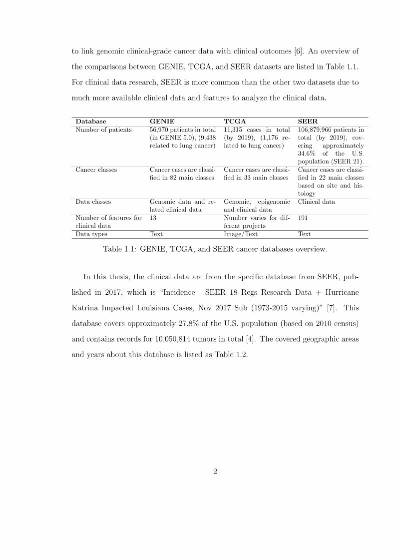
to link genomic clinical-grade cancer data with clinical outcomes [6]. An overview of

the comparisons between GENIE, TCGA, and SEER datasets are listed in Table 1.1.

For clinical data research, SEER is more common than the other two datasets due to

much more available clinical data and features to analyze the clinical data.

Database GENIE TCGA SEERNumber of patients 56,970 patients in total

(in GENIE 5.0), (9,438related to lung cancer)

11,315 cases in total(by 2019), (1,176 re-lated to lung cancer)

106,879,966 patients intotal (by 2019), cov-ering approximately34.6% of the U.S.population (SEER 21).

Cancer classes Cancer cases are classi-fied in 82 main classes

Cancer cases are classi-fied in 33 main classes

Cancer cases are classi-fied in 22 main classesbased on site and his-tology

Data classes Genomic data and re-lated clinical data

Genomic, epigenomicand clinical data

Clinical data

Number of features forclinical data

13 Number varies for dif-ferent projects

191

Data types Text Image/Text Text

Table 1.1: GENIE, TCGA, and SEER cancer databases overview.

In this thesis, the clinical data are from the specific database from SEER, pub-

lished in 2017, which is “Incidence - SEER 18 Regs Research Data + Hurricane

Katrina Impacted Louisiana Cases, Nov 2017 Sub (1973-2015 varying)” [7]. This

database covers approximately 27.8% of the U.S. population (based on 2010 census)

and contains records for 10,050,814 tumors in total [4]. The covered geographic areas

and years about this database is listed as Table 1.2.

2

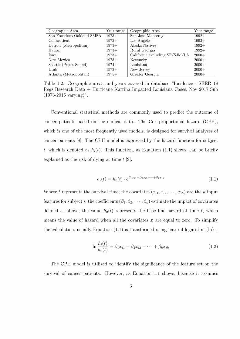
Geographic Area Year range Geographic Area Year rangeSan Francisco-Oakland SMSA 1973+ San Jose-Monterey 1992+Connecticut 1973+ Los Angeles 1992+Detroit (Metropolitan) 1973+ Alaska Natives 1992+Hawaii 1973+ Rural Georgia 1992+Iowa 1973+ California excluding SF/SJM/LA 2000+New Mexico 1973+ Kentucky 2000+Seattle (Puget Sound) 1974+ Louisiana 2000+Utah 1973+ New Jersey 2000+Atlanta (Metropolitan) 1975+ Greater Georgia 2000+

Table 1.2: Geographic areas and years covered in database “Incidence - SEER 18Regs Research Data + Hurricane Katrina Impacted Louisiana Cases, Nov 2017 Sub(1973-2015 varying)”.

Conventional statistical methods are commonly used to predict the outcome of

cancer patients based on the clinical data. The Cox proportional hazard (CPH),

which is one of the most frequently used models, is designed for survival analyses of

cancer patients [8]. The CPH model is expressed by the hazard function for subject

i, which is denoted as hi(t). This function, as Equation (1.1) shows, can be briefly

explained as the risk of dying at time t [9].

hi(t) = h0(t) · eβ1xi1+β2xi2+···+βkxik (1.1)

Where t represents the survival time; the covariates (xi1, xi2, · · · , xik) are the k input

features for subject i; the coefficients (β1, β2, · · · , βk) estimate the impact of covariates

defined as above; the value h0(t) represents the base line hazard at time t, which

means the value of hazard when all the covariates x are equal to zero. To simplify

the calculation, usually Equation (1.1) is transformed using natural logarithm (ln) :

lnhi(t)

h0(t)= β1xi1 + β2xi2 + · · ·+ βkxik (1.2)

The CPH model is utilized to identify the significance of the feature set on the

survival of cancer patients. However, as Equation 1.1 shows, because it assumes

3

that the outcome is a linear combination of covariates x , it is too simple to predict

cancer patients’ outcomes accurately, leading to insufficient or unnecessary treatment,

because the outcomes of patients usually have complex interactions and relationships

between variables.

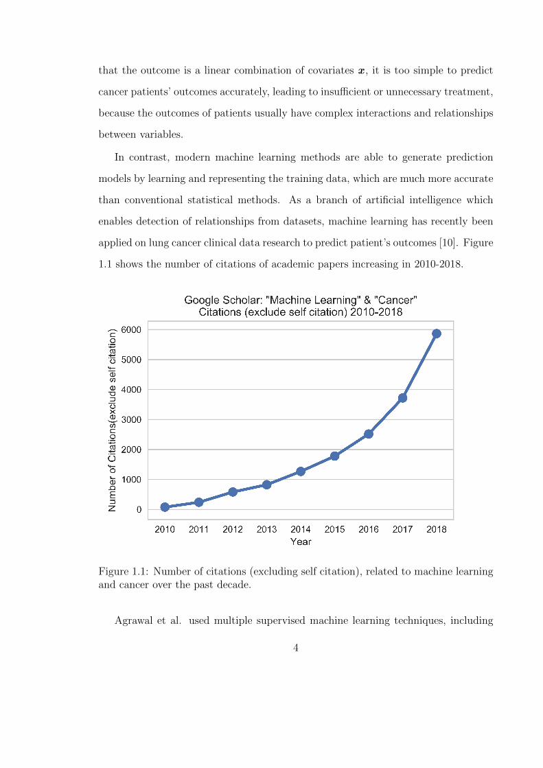
In contrast, modern machine learning methods are able to generate prediction

models by learning and representing the training data, which are much more accurate

than conventional statistical methods. As a branch of artificial intelligence which

enables detection of relationships from datasets, machine learning has recently been

applied on lung cancer clinical data research to predict patient’s outcomes [10]. Figure

1.1 shows the number of citations of academic papers increasing in 2010-2018.

Figure 1.1: Number of citations (excluding self citation), related to machine learningand cancer over the past decade.

Agrawal et al. used multiple supervised machine learning techniques, including

4

support vector machines, artificial neural networks, decision trees, random forests,

and others to analyze the survivability of lung cancer patients and compare the per-

formance of these methods on data from the the SEER database. In their paper, they

also designed an online user-friendly outcome calculator for patients, which does not

need professional knowledge to use [11].

Lynch et al. applied a number of supervised learning techniques to the Surveil-

lance, Epidemiology, and End Results program (SEER) [3] database to classify lung

cancer patients in terms of survival, including the techniques of linear regression, de-

cision trees, and gradient boosting machines (GBM)[12]. Lynch et al. also applied

some unsupervised machine learning techniques for classification and clustering to a

collection of descriptive variables from 10,442 lung cancer patient records in the SEER

database. Their results show unsupervised data analysis techniques may be of use

to classify patients by defining the classes as effective proxies for survival prediction

[13].

Wang et al. proposed a two-stage machine learning model to enhance cancer

survival prediction based on a decision tree-based imbalanced ensemble classification

method and a selective ensemble regression method. This approach can effectively

handle the imbalanced colorectal cancer data from the SEER database, and the pro-

posed regression method outperforms several state-of-the-art methods [14]

Machine learning methods as listed above have made remarkable achievements

in analyzing large sets of clinical data to draw conclusions and make predictions to

determine the survivability of a specific lung cancer patient. However, as the sizes of

the datasets continue to grow, predicting lung cancer patients’ outcomes may become

an increasingly difficult problem, because of two main reasons: one relates to the

number of samples for training, the other is its model complexity which is related

to the execution time of certain methods. As such, there is a strong motivation to

5

develop efficient methods to analyze clinical data accurately.

A new ensemble method based on the decision tree, named as GCForest, was first

introduced and implemented by Zhou and his colleagues [15]. GCForest shows a good

performance on different tasks involving image and text input for classification and

regression. This thesis focuses on making meaningful predictions and evaluation with

the input of data from the SEER clinical database by using the GCForest ensemble

decision tree methods.

This thesis is organized in the following manner. In Chapter 2, a brief overview

of typical machine learning methods is given for context. Chapter 3 introduces the

development of ensemble methods and deep forests. Chapter 4 shows the implementa-

tion of a deep forest method which is optimized for clinical data and compares it with

respect to training efficiency and classification accuracy to conventional ML methods,

including support vector machine, random forests, and deep neural networks. Finally,

Chapter 5 presents conclusions and suggests future work.

6

Chapter 2: Overview of Machine Learning Techniques

Providing the ability to automatically recognize unknown patterns and create high

performing predictive models from data, machine learning, especially deep learning,

is a very hot topic with many applications in recent years [16]. Based on the kind

of data available and the specific research task, machine learning can be generally

divided into at least three types [17]:

• Supervised learning. The machine learning model learns on a labeled dataset,

with the labels providing values associated with each data item that the algo-

rithm can use in model construction and to evaluate the constructed model’s

accuracy by comparing the model’s predicted labels/values to the actual label-

s/values on a test set (a subset of the the dataset).

• Unsupervised learning. The machine learning model attempts to extract fea-

tures and patterns on its own from unlabeled input data.

• Reinforcement learning. The machine learning model learns the training dataset

with a reward system. A reward feedback will be provided to the base learner

when it performs a better action in a particular situation.

2.1 Supervised Learning

2.1.1 Notational Conventions and Types of Supervised Learning

As described earlier, supervised learning model uses two different datasets, training

set S and test set T . They are generated from datasetD, usually using hold-out, cross-

validation, and bootstrap. After training the model using S, test error is evaluated

by applying the model on T , to estimate the model’s generalization error in real

7

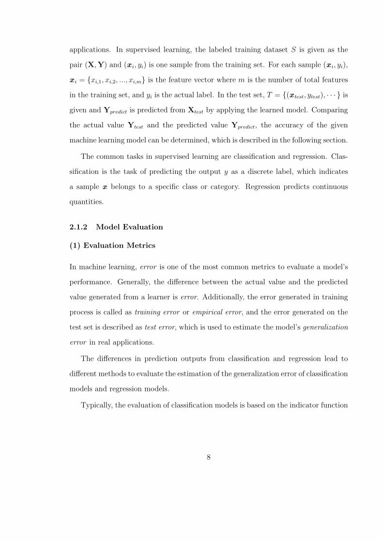
applications. In supervised learning, the labeled training dataset S is given as the

pair (X,Y) and (x i, yi) is one sample from the training set. For each sample (x i, yi),

x i = {xi,1, xi,2, ..., xi,m} is the feature vector where m is the number of total features

in the training set, and yi is the actual label. In the test set, T = {(x test, ytest), · · · } is

given and Ypredict is predicted from Xtest by applying the learned model. Comparing

the actual value Ytest and the predicted value Ypredict, the accuracy of the given

machine learning model can be determined, which is described in the following section.

The common tasks in supervised learning are classification and regression. Clas-

sification is the task of predicting the output y as a discrete label, which indicates

a sample x belongs to a specific class or category. Regression predicts continuous

quantities.

2.1.2 Model Evaluation

(1) Evaluation Metrics

In machine learning, error is one of the most common metrics to evaluate a model’s

performance. Generally, the difference between the actual value and the predicted

value generated from a learner is error. Additionally, the error generated in training

process is called as training error or empirical error, and the error generated on the

test set is described as test error, which is used to estimate the model’s generalization

error in real applications.

The differences in prediction outputs from classification and regression lead to

different methods to evaluate the estimation of the generalization error of classification

models and regression models.

Typically, the evaluation of classification models is based on the indicator function

8

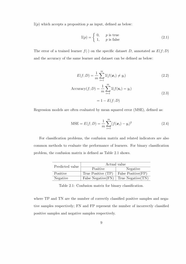
I(p) which accepts a proposition p as input, defined as below:

I(p) =

{0, p is true1, p is false

(2.1)

The error of a trained learner f(·) on the specific dataset D, annotated as E(f ;D)

and the accuracy of the same learner and dataset can be defined as below:

E(f ;D) =1

m

m∑i=1

I(f(x i) 6= yi) (2.2)

Accuracy(f ;D) =1

m

m∑i=1

I(f(xi) = yi)

= 1− E(f ;D)

(2.3)

Regression models are often evaluated by mean squared error (MSE), defined as:

MSE = E(f ;D) =1

m

m∑i=1

(f(x i)− yi)2 (2.4)

For classification problems, the confusion matrix and related indicators are also

common methods to evaluate the performance of learners. For binary classification

problem, the confusion matrix is defined as Table 2.1 shows.

Predicted valueActual value

Positive NegativePositive True Positive (TP) False Positive(FP)Negative False Negative(FN) True Negative(TN)

Table 2.1: Confusion matrix for binary classification.

where TP and TN are the number of correctly classified positive samples and nega-

tive samples respectively; FN and FP represent the number of incorrectly classified

positive samples and negative samples respectively.

9

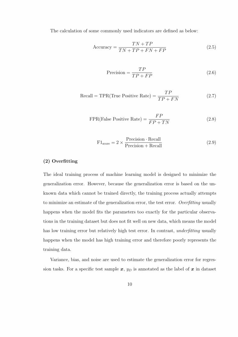
The calculation of some commonly used indicators are defined as below:

Accuracy =TN + TP

TN + TP + FN + FP(2.5)

Precision =TP

TP + FP(2.6)

Recall = TPR(True Positive Rate) =TP

TP + FN(2.7)

FPR(False Positive Rate) =FP

FP + TN(2.8)

F1score = 2× Precision · Recall

Precision + Recall(2.9)

(2) Overfitting

The ideal training process of machine learning model is designed to minimize the

generalization error. However, because the generalization error is based on the un-

known data which cannot be trained directly, the training process actually attempts

to minimize an estimate of the generalization error, the test error. Overfitting usually

happens when the model fits the parameters too exactly for the particular observa-

tions in the training dataset but does not fit well on new data, which means the model

has low training error but relatively high test error. In contrast, underfitting usually

happens when the model has high training error and therefore poorly represents the

training data.

Variance, bias, and noise are used to estimate the generalization error for regres-

sion tasks. For a specific test sample x , yD is annotated as the label of x in dataset

10

D, y is annotated as the actual label of x . f(x ;D) is the prediction on dataset D

with input x , which is an estimation of actual model f . Then, the expectation E of

f(x ) and D is :

f (x ) = ED [f (x ;D)] (2.10)

The variance by using different training sets which have the same size, denoted as

var(x ), indicating the impact of changing data, is defined as below.

var(x ) = ED[(f (x ;D)− f (x )

)2](2.11)

The noise is defined as below, which represents the lower boundary of the gener-

alization error:

ε2 = ED[(yD − y)2

](2.12)

The bias is defined as the distance between predicted output and the actual output,

which represents the fitting ability of a specific learner:

bias2(x ) = (f(x )− y)2 (2.13)

In order to analyze the generalization error, Geman et at. implemented bias-

variance decomposition in 1992, dividing the generalization error into three parts:

bias, variance, and noise, as Equation (2.14) shows: [18].

E(f ;D) = bias2(x ) + var(x ) + ε2 (2.14)

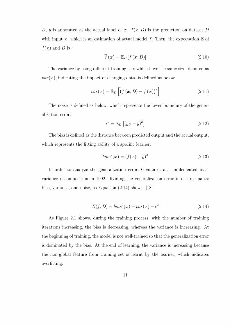
As Figure 2.1 shows, during the training process, with the number of training

iterations increasing, the bias is decreasing, whereas the variance is increasing. At

the beginning of training, the model is not well-trained so that the generalization error

is dominated by the bias. At the end of learning, the variance is increasing because

the non-global feature from training set is learnt by the learner, which indicates

overfitting.

11

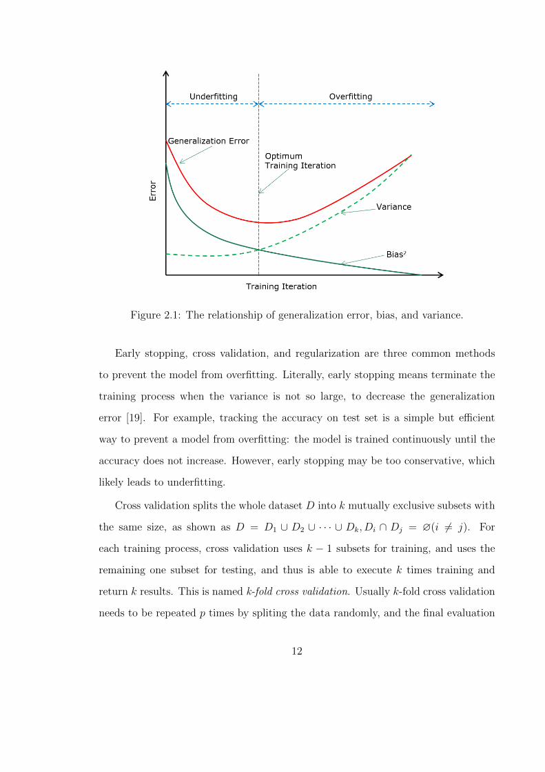
Figure 2.1: The relationship of generalization error, bias, and variance.

Early stopping, cross validation, and regularization are three common methods

to prevent the model from overfitting. Literally, early stopping means terminate the

training process when the variance is not so large, to decrease the generalization

error [19]. For example, tracking the accuracy on test set is a simple but efficient

way to prevent a model from overfitting: the model is trained continuously until the

accuracy does not increase. However, early stopping may be too conservative, which

likely leads to underfitting.

Cross validation splits the whole dataset D into k mutually exclusive subsets with

the same size, as shown as D = D1 ∪ D2 ∪ · · · ∪ Dk, Di ∩ Dj = ∅(i 6= j). For

each training process, cross validation uses k − 1 subsets for training, and uses the

remaining one subset for testing, and thus is able to execute k times training and

return k results. This is named k-fold cross validation. Usually k-fold cross validation

needs to be repeated p times by spliting the data randomly, and the final evaluation

12

is based on the mean of k-fold cross validation repeated p times.

Regularization aims to decrease the model complexity by adding a regularization

term or penalty term to the loss function, in order to reduce the risk of overfitting.

The base form of the regularization term is given as L(w) where w is related to

the weight of each feature input, and the regularization term is able to represent the

number of non-zero term in w . One of the common regularization term is L2 norm,

defined as follows:

L2 : ‖w‖2 =

√√√√ m∑i=1

w2i (2.15)

Another regularization term is L1 norm, with simply replacing the sum of square of

weights to the sum of absolute value of weights, defined as below:

L1 : ‖w‖1 =m∑i=1

|wi| (2.16)

Very interestingly, regularization is also used in dimensional reduction. Least

absolute shrinkage and selection operator (Lasso) [20] performs both feature selection

and regularization in order to enhance the prediction accuracy and interpretability of

the machine learning model it produces. Lasso applies L1 norm on the loss function

of linear regression model, which decreases the risk of overfitting.

minw

m∑i=1

(yi −wTx i

)2+ λ‖w‖1. (2.17)

where D = {(x 1, y1), (x 2, y2), · · · , (xm, ym)} is the input set of samples, and w =

{w1, w2, · · · , wn} are defined as Lasso coefficients, which reflect the importance of the

related feature xi ∈ x , i = 1, 2, · · · , n to target y .

13

2.1.3 Decision Tree

Decision tree is a very common method in machine learning. A decision tree can be

“learned” by splitting the original set into subsets based on the information gain. The

procedure of generating a decision tree is based on divide-and-conquer.

Assume the k-th class xk in whole dataset D has frequency pk, (k = 1, 2, ...,m),

the information gain of D is

IG(D, a) = I(D)−V∑v=1

|Dv||D|

I(Dv) (2.18)

Here I(D) is the impurity of D, which can be implemented in multiple ways. Suppos-

ing the discrete feature a has V possible values {a1, a2, ..., aV }, if feature a is used to

split the dataset D, it will generate V sub-nodes, where the v-th sub-node contains

a subset of D, annotated as Dv = {x ∈ a | x = av}. The larger value of information

gain indicates the larger purity of D.

The basic algorithm is given as the pseudo code below:

14

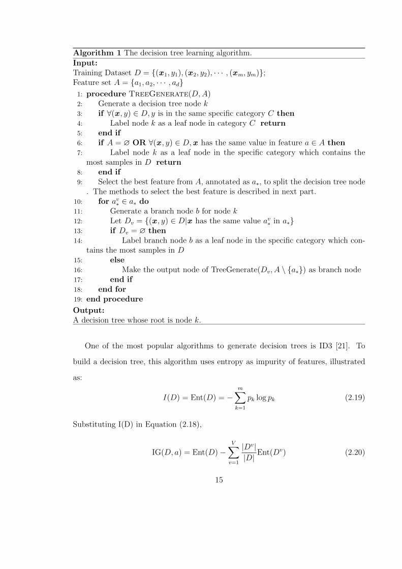
Algorithm 1 The decision tree learning algorithm.Input:Training Dataset D = {(x 1, y1), (x 2, y2), · · · , (xm, ym)};Feature set A = {a1, a2, · · · , ad}

1: procedure TreeGenerate(D,A)2: Generate a decision tree node k3: if ∀(x , y) ∈ D, y is in the same specific category C then4: Label node k as a leaf node in category C return5: end if6: if A = ∅ OR ∀(x , y) ∈ D,x has the same value in feature a ∈ A then7: Label node k as a leaf node in the specific category which contains the

most samples in D return8: end if9: Select the best feature from A, annotated as a∗, to split the decision tree node. The methods to select the best feature is described in next part.

10: for av∗ ∈ a∗ do11: Generate a branch node b for node k12: Let Dv = {(x , y) ∈ D|x has the same value av∗ in a∗}13: if Dv = ∅ then14: Label branch node b as a leaf node in the specific category which con-

tains the most samples in D15: else16: Make the output node of TreeGenerate(Dv, A \ {a∗}) as branch node17: end if18: end for19: end procedure

Output:A decision tree whose root is node k.

One of the most popular algorithms to generate decision trees is ID3 [21]. To

build a decision tree, this algorithm uses entropy as impurity of features, illustrated

as:

I(D) = Ent(D) = −m∑k=1

pk log pk (2.19)

Substituting I(D) in Equation (2.18),

IG(D, a) = Ent(D)−V∑v=1

|Dv||D|

Ent(Dv) (2.20)

15

To split a decision tree node, the optimal solution is using feature a∗, which brings

the maximum of information gain:

a∗ = argmaxa∈A

IG(D, a) (2.21)

Another popular method to split the decision tree node is Classification And

Regression Trees (CART) [22]. In this method, the Gini value is used to indicate the

purity of D.

Gini(D) =m∑k=1

∑k′ 6=k

pkpk′

= 1−m∑k=1

pk2

(2.22)

From the equation, Gini(D) indicates the probability of randomly choosing 2 different

samples from D. Smaller values of Gini(D) means higher purity of D. The Gini

index of feature a could be treated as the impurity of dataset D, and it is defined by

substituting I(D) in Equation (2.18) with Gini(D):

IG(D, a) = Gini index(D, a) = 1−V∑v=1

|Dv||D|

Gini(Dv) (2.23)

So the best feature to split the decision node can be annotated as:

a∗ = argmaxa∈A

IG(D, a) (2.24)

Figure 2.2 shows a constructed CART decision tree, trained on the Iris dataset

[23]. In this CART, Gini index is used to split the tree node. For example, when

splitting the root node, the attribute and the value in this attribute with the minimum

Gini index, “petal width” and “0.8”, are selected. Then the root node is divided into

two nodes by the condition “petal width ≤ 0.8”. Applying the split process to all

nodes recursively, a decision tree illustrated as Figure 2.2 is generated.

16

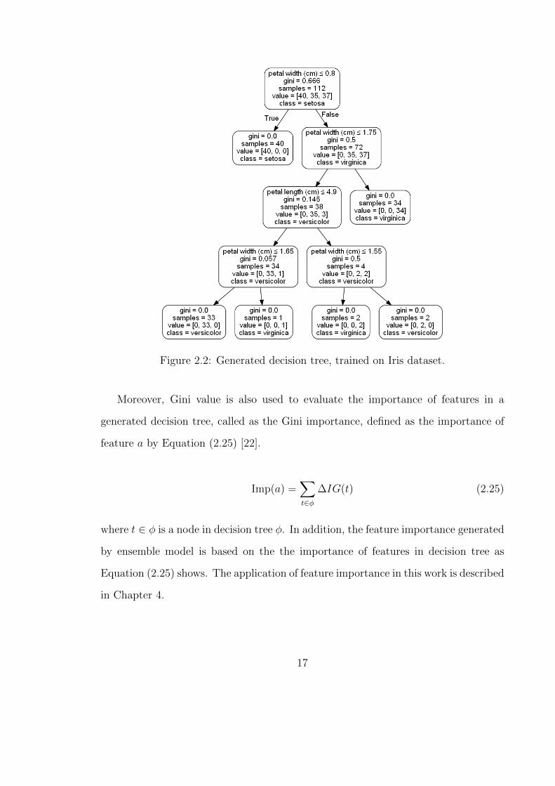
Figure 2.2: Generated decision tree, trained on Iris dataset.

Moreover, Gini value is also used to evaluate the importance of features in a

generated decision tree, called as the Gini importance, defined as the importance of

feature a by Equation (2.25) [22].

Imp(a) =∑t∈φ

∆IG(t) (2.25)

where t ∈ φ is a node in decision tree φ. In addition, the feature importance generated

by ensemble model is based on the the importance of features in decision tree as

Equation (2.25) shows. The application of feature importance in this work is described

in Chapter 4.

17

2.1.4 Support Vector Machine

Support vector machines (SVM), first introduced in 1963 [24], is a well established

supervised machine learning algorithm. SVM has been widely used in cancer data

research. Listgarten et al. used SVM to analyze the susceptibility of breast cancer

for multiple treatments [25]. Ehlers and Harbour applied SVM model on genomic

cancer data to rank the 25 primary uveal melanomas tumors, in order to find the

correlations between the ranking of uveal melanomas tumors and NBS1 protein [26].

The main idea of SVM is to construct some hyperplanes in a high-dimensional

space for classification, or regression, by attempting maximize the distance, as known

as margin, from hyperplanes to the nearest point of input data. The hyperplane

dividing different classes is usually described as:

wTx + b = 0 (2.26)

where w = {w1, w2, · · · , wn} is the normal vector which determines the direction of

the hyperplane, and b determines the distance from that hyperplane to the origin

of the multi-dimensional space. So the distance r from one sample x ∈ X to the

hyperplane (w , b) is given as:

r =|wTx+ b|‖w‖

. (2.27)

where ‖w‖ is the Euclidean norm of w , as Equation (2.28) shows.

‖w‖ =

√√√√ n∑i=1

wi2 (2.28)

Ideally, the hyperplane (w , b) can divide all of the training data correctly, which

18

means that for each pair of (x i, yi) ∈ D:

{wTx + b ≥ +1, yi = +1wTx + b ≤ −1, yi = −1

(2.29)

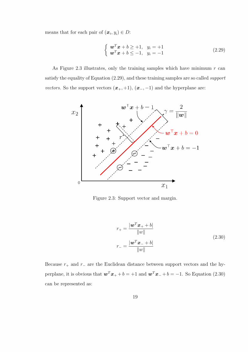
As Figure 2.3 illustrates, only the training samples which have minimum r can

satisfy the equality of Equation (2.29), and these training samples are so called support

vectors. So the support vectors (x+,+1), (x−,−1) and the hyperplane are:

Figure 2.3: Support vector and margin.

r+ =|wTx+ + b|‖w‖

r− =|wTx− + b|‖w‖

(2.30)

Because r+ and r− are the Euclidean distance between support vectors and the hy-

perplane, it is obvious that wTx+ + b = +1 and wTx−+ b = −1. So Equation (2.30)

can be represented as:

19

r+ =|+ 1|‖w‖

r− =| − 1|‖w‖

(2.31)

The sum of distance γ of support vectors from two different categories, as known

as margin, for these two categories, is defined as below:

γ = r+ + r−

=2

‖w‖

(2.32)

SVM attempts to find the hyperplane which has the maximum margin, i.e. to

find a specific pair of (w , b) to let γ achieve its maximum, as Equation (2.33) shows:

maxw ,b

2

‖w‖

s.t. yi(wTx i + b) ≥ 1, i = 1, 2, · · · ,m

(2.33)

In order to maximize the margin as Equation (2.33) shows, ‖w‖−1 needs to be

maximized, which is equivalent to minimizing ‖w‖2. So Equation (2.33) can be recast

as below, which is the standard form of SVM.

minw ,b

1

2‖w‖2

s.t. yi(wTx i + b) ≥ 1, i = 1, 2, · · · ,m

(2.34)

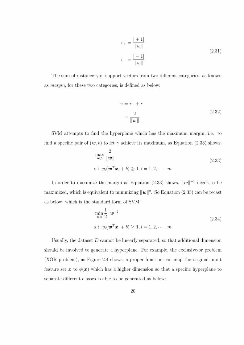
Usually, the dataset D cannot be linearly separated, so that additional dimension

should be involved to generate a hyperplane. For example, the exclusive-or problem

(XOR problem), as Figure 2.4 shows, a proper function can map the original input

feature set x to φ(x ) which has a higher dimension so that a specific hyperplane to

separate different classes is able to be generated as below:

20

Figure 2.4: XOR problem using SVM.

f(x ) = wTφ(x ) + b (2.35)

Then, similar to Equation (2.34), the problem to find the optimal hyperplane in

mapped feature set φ(x ) can be described as:

minw ,b

1

2‖w‖2

s.t. yi(wTφ(x i) + b) ≥ 1, i = 1, 2, · · · ,m

(2.36)

The original problem on φ(x ), Equation (2.36), can be transformed in dual space

by means of Lagrangian [27]. The transformed problem is given as below, and the α

here is Lagrangian multiplier.

21

maxα

m∑i=1

αi −1

2

m∑i=1

m∑j=1

αiαjyiyjφ(x i)Tφ(x j)

s.t.m∑i=1

αiyi = 0,

αi ≥ 0, i = 1, 2, · · · ,m

(2.37)

Usually, the calculation of φ(x i)Tφ(x j) is difficult because φ(x ) may have a

very high dimension. So kernel tricks, mapping the original features to the higher-

dimension to make the separation easier, was introduced in 1992 by B. Boser et al

[27]. The key point of kernel tricks is to find a function K(·, ·) and let K(x i,x j) =

φ(x i)Tφ(x j). The function K(·, ·) is a so-called kernel function. Then the Equation

(2.37) can be written as:

maxα

m∑i=1

αi −1

2

m∑i=1

m∑j=1

αiαjyiyjK(x i,x j)

s.t.m∑i=1

αiyi = 0,

αi ≥ 0, i = 1, 2, · · · ,m

(2.38)

The optimal coefficients of the hyperplane, as Equation (2.39) shows, is the so-

lution of Equation (2.38). The optimal solution can be accessed by expanding and

calculating the kernel function K(·, ·) on training samples, known as support vector

expansion.

f(x ) = wTφ(x ) + b

=m∑i

αiyiK(x ,x i) + b.(2.39)

22

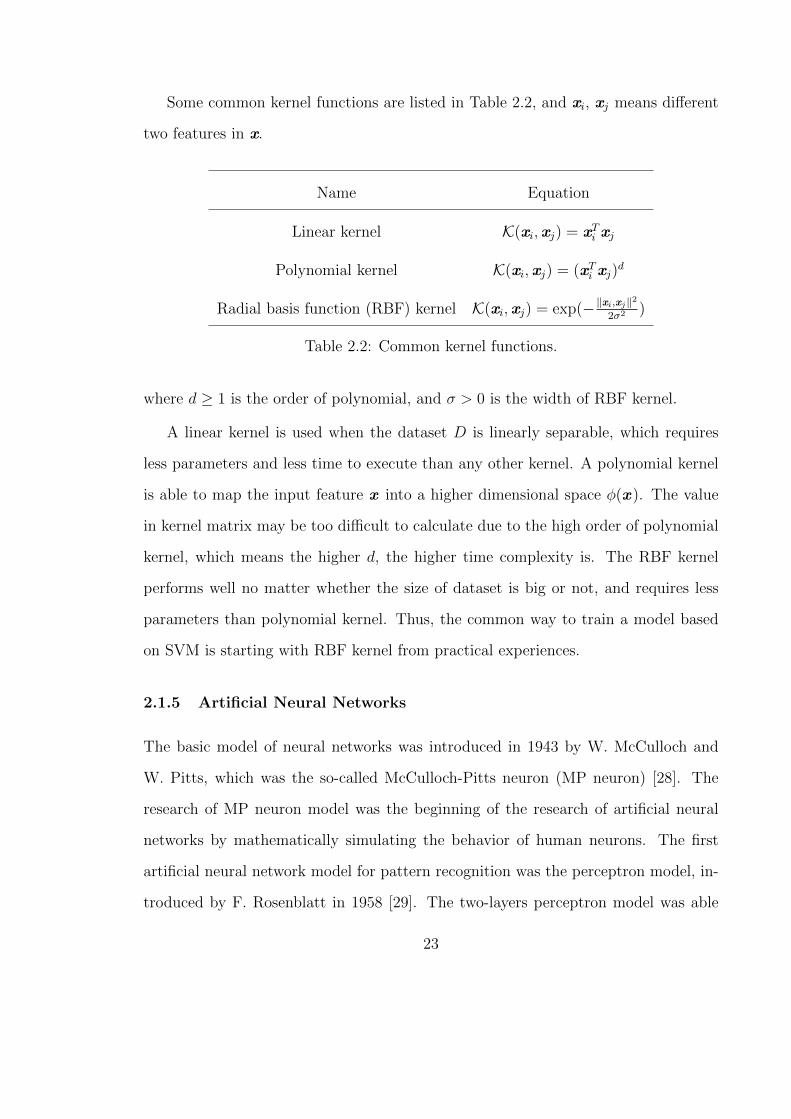
Some common kernel functions are listed in Table 2.2, and xi, xj means different

two features in x.

Name Equation

Linear kernel K(xi,xj) = xTi xj

Polynomial kernel K(xi,xj) = (xTi xj)d

Radial basis function (RBF) kernel K(xi,xj) = exp(−‖xi,xj‖2

2σ2 )

Table 2.2: Common kernel functions.

where d ≥ 1 is the order of polynomial, and σ > 0 is the width of RBF kernel.

A linear kernel is used when the dataset D is linearly separable, which requires

less parameters and less time to execute than any other kernel. A polynomial kernel

is able to map the input feature x into a higher dimensional space φ(x ). The value

in kernel matrix may be too difficult to calculate due to the high order of polynomial

kernel, which means the higher d, the higher time complexity is. The RBF kernel

performs well no matter whether the size of dataset is big or not, and requires less

parameters than polynomial kernel. Thus, the common way to train a model based

on SVM is starting with RBF kernel from practical experiences.

2.1.5 Artificial Neural Networks

The basic model of neural networks was introduced in 1943 by W. McCulloch and

W. Pitts, which was the so-called McCulloch-Pitts neuron (MP neuron) [28]. The

research of MP neuron model was the beginning of the research of artificial neural

networks by mathematically simulating the behavior of human neurons. The first

artificial neural network model for pattern recognition was the perceptron model, in-

troduced by F. Rosenblatt in 1958 [29]. The two-layers perceptron model was able

23

to generate output by applying arithmetic operations on inputs. One major improve-

ment of neural networks was Back Propagation, introduced by P. Werbos in 1974 and

successfully applied in LeNet recognize to handwritten zip-code by Y. LeCun et al.

in 1989 [30]. During the 1990s, with the development of SVM, the improvement of

neural networks temporarily stalled due to the large amount of calculations required.

In 2012, A. Krizhevsky et al. developed AlexNet [31] using CUDA [32] based on

GPU to accelerate the training process of neural networks, and made a huge success

in ImageNet [33] classification, which is now often recognized as the beginning of deep

learning trend.

The following parts describe the structure of artificial neural networks in detail.

(1) Artificial Neuron

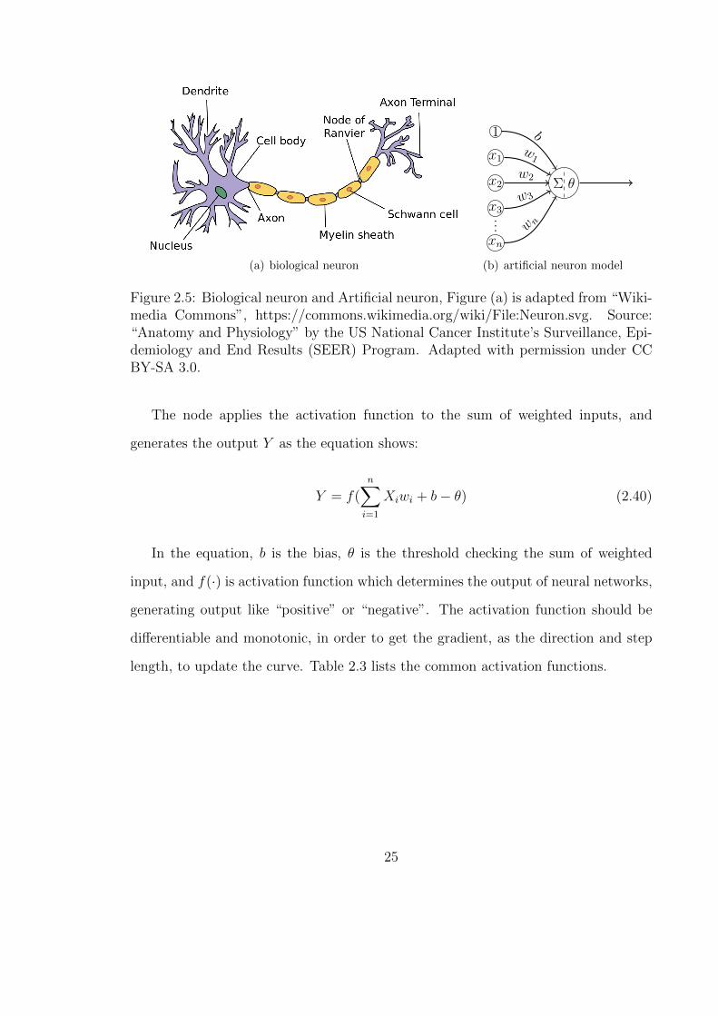
Artificial neural networks are inspired by the behavior of biological neural networks in

brain and neural science [34]. With the similar layer-by-layer structure like biological

neural systems as Figure 2.5(a) shows, the neural network is able to “generate a

response” on the basis of stimulation input. The basic unit in a neural network is

the neuron, also called as a node or a unit, which is from the MP neuron model. As

Figure 2.5(b) shows, each input xi has an associated weight (wi), which indicates the

relative importance of this input as compared to other inputs.

24

(a) biological neuron

Σ θ

1

x1

x2

x3

xn

bw1

w2

w3

w n

...

(b) artificial neuron model

Figure 2.5: Biological neuron and Artificial neuron, Figure (a) is adapted from “Wiki-media Commons”, https://commons.wikimedia.org/wiki/File:Neuron.svg. Source:“Anatomy and Physiology” by the US National Cancer Institute’s Surveillance, Epi-demiology and End Results (SEER) Program. Adapted with permission under CCBY-SA 3.0.

The node applies the activation function to the sum of weighted inputs, and

generates the output Y as the equation shows:

Y = f(n∑i=1

Xiwi + b− θ) (2.40)

In the equation, b is the bias, θ is the threshold checking the sum of weighted

input, and f(·) is activation function which determines the output of neural networks,

generating output like “positive” or “negative”. The activation function should be

differentiable and monotonic, in order to get the gradient, as the direction and step

length, to update the curve. Table 2.3 lists the common activation functions.

25

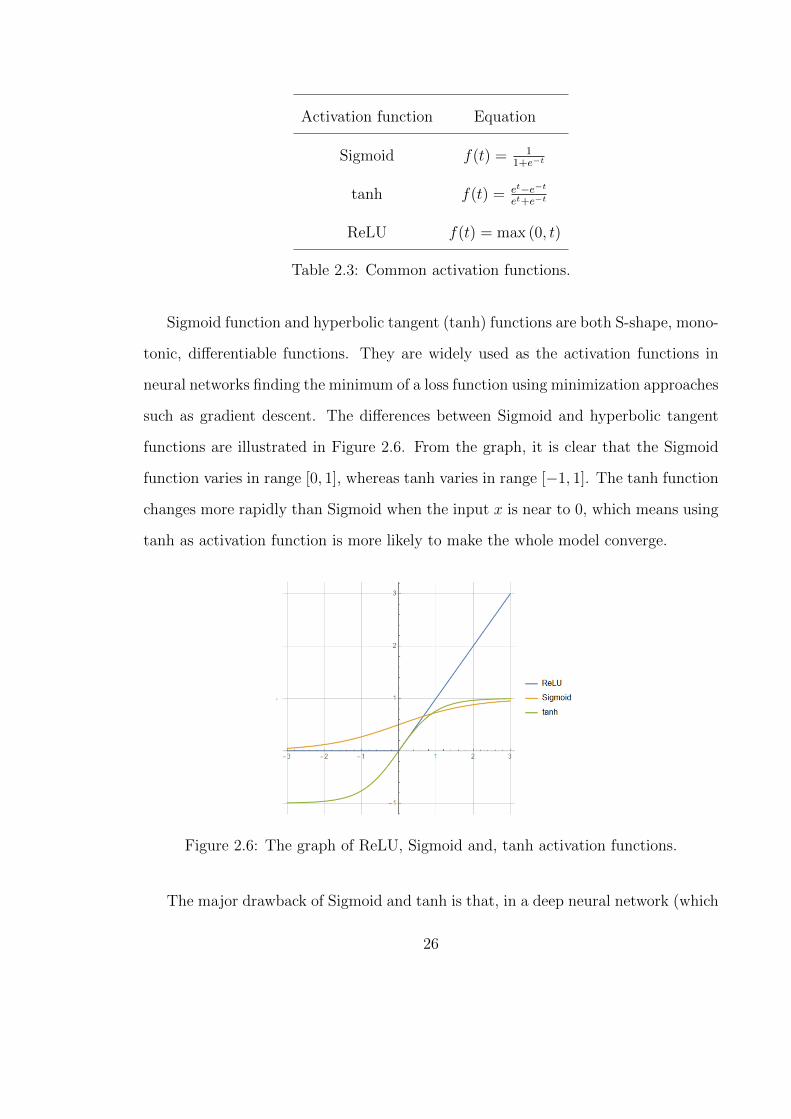
Activation function Equation

Sigmoid f(t) = 11+e−t

tanh f(t) = et−e−t

et+e−t

ReLU f(t) = max (0, t)

Table 2.3: Common activation functions.

Sigmoid function and hyperbolic tangent (tanh) functions are both S-shape, mono-

tonic, differentiable functions. They are widely used as the activation functions in

neural networks finding the minimum of a loss function using minimization approaches

such as gradient descent. The differences between Sigmoid and hyperbolic tangent

functions are illustrated in Figure 2.6. From the graph, it is clear that the Sigmoid

function varies in range [0, 1], whereas tanh varies in range [−1, 1]. The tanh function

changes more rapidly than Sigmoid when the input x is near to 0, which means using

tanh as activation function is more likely to make the whole model converge.

Figure 2.6: The graph of ReLU, Sigmoid and, tanh activation functions.

The major drawback of Sigmoid and tanh is that, in a deep neural network (which

26

has multiple layers), the gradient may be too small to update a new value. As a result,

the model converges very slowly and this is the so called vanishing gradient problem.

Motivated by the vanishing gradient problem, the Rectified Linear Unit (ReLU) is an

activation function defined by a constant positive gradient value 1 for positive inputs,

and 0 for negative inputs [35], as Equation (2.41) shows:

f (x) =

{x, x > 00, x ≤ 0

(2.41)

When a ReLU is activated with input above 0, the partial derivative is 1, which is able

to make ReLU avoid the vanishing gradient problem in multi-layer neural networks.

If the input x ≤ 0, the gradient of ReLU will be a constant 0, which is also described

as a saturated ReLU.

However, ReLUs have potential disadvantage during the training process because

the gradient is constantly 0 when the input is negative, which are called as the satu-

rated ReLU. This could result in slow convergence of model because saturated ReLU

never activates so that a gradient-based method will not adjust its weights, which is

the so-called “dying ReLU problem”.

To alleviate the potential dying ReLU problems caused by constant 0, a possible

solution is using leaky ReLU [36], a typical variant for ReLU, defined as below:

f (x) =

{x, x > 0

0.01x, x ≤ 0(2.42)

Leaky ReLU has a relatively smaller gradient for negative inputs, compared with pos-

itive inputs. This feature allows a gradient optimizing method to adjust the weights

slightly and slowly when leaky ReLU is saturated and not active to avoid becoming

the dying ReLU.

27

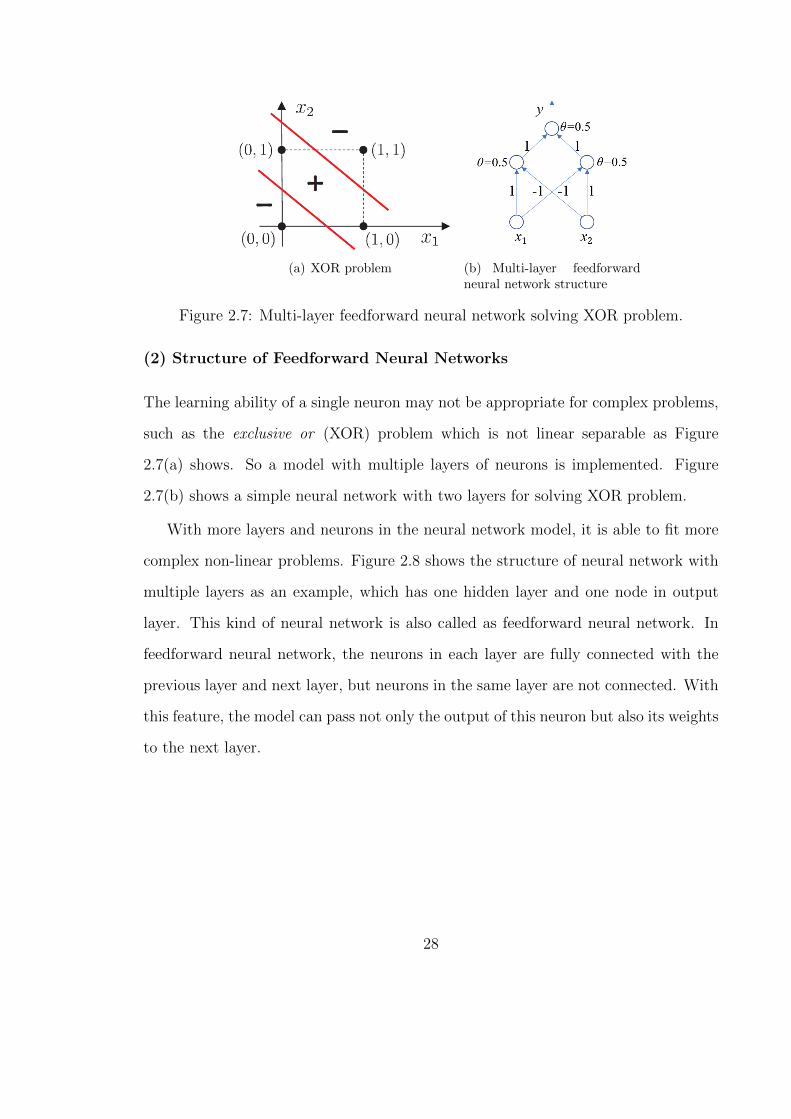
(a) XOR problem (b) Multi-layer feedforwardneural network structure

Figure 2.7: Multi-layer feedforward neural network solving XOR problem.

(2) Structure of Feedforward Neural Networks

The learning ability of a single neuron may not be appropriate for complex problems,

such as the exclusive or (XOR) problem which is not linear separable as Figure

2.7(a) shows. So a model with multiple layers of neurons is implemented. Figure

2.7(b) shows a simple neural network with two layers for solving XOR problem.

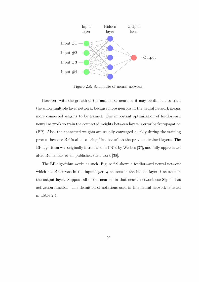
With more layers and neurons in the neural network model, it is able to fit more

complex non-linear problems. Figure 2.8 shows the structure of neural network with

multiple layers as an example, which has one hidden layer and one node in output

layer. This kind of neural network is also called as feedforward neural network. In

feedforward neural network, the neurons in each layer are fully connected with the

previous layer and next layer, but neurons in the same layer are not connected. With

this feature, the model can pass not only the output of this neuron but also its weights

to the next layer.

28

Input #1

Input #2

Input #3

Input #4

Output

Hiddenlayer

Inputlayer

Outputlayer

Figure 2.8: Schematic of neural network.

However, with the growth of the number of neurons, it may be difficult to train

the whole multiple layer network, because more neurons in the neural network means

more connected weights to be trained. One important optimization of feedforward

neural network to train the connected weights between layers is error backpropagation

(BP). Also, the connected weights are usually converged quickly during the training

process because BP is able to bring “feedbacks” to the previous trained layers. The

BP algorithm was originally introduced in 1970s by Werbos [37], and fully appreciated

after Rumelhart et al. published their work [38].

The BP algorithm works as such. Figure 2.9 shows a feedforward neural network

which has d neurons in the input layer, q neurons in the hidden layer, l neurons in

the output layer. Suppose all of the neurons in that neural network use Sigmoid as

activation function. The definition of notations used in this neural network is listed

in Table 2.4.

29

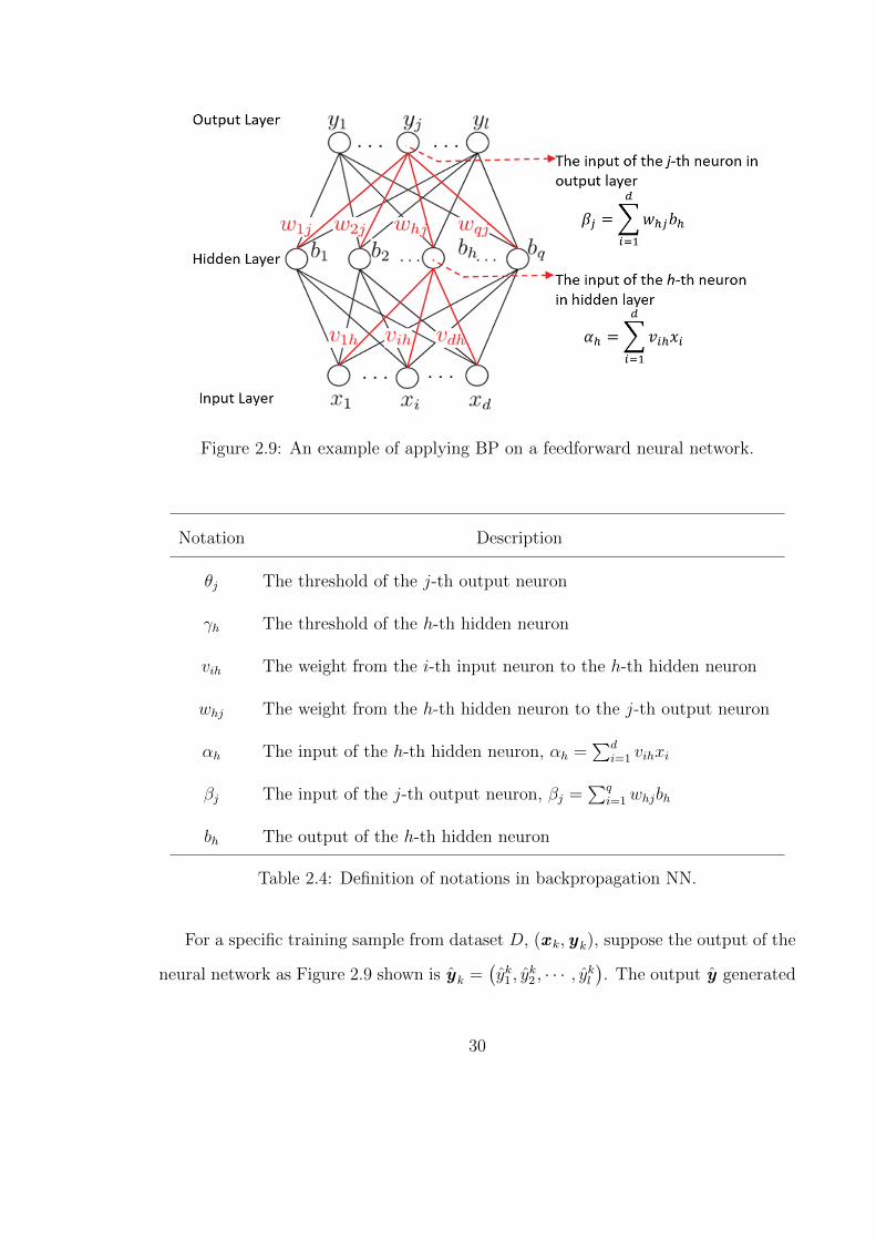
Figure 2.9: An example of applying BP on a feedforward neural network.

Notation Description

θj The threshold of the j-th output neuron

γh The threshold of the h-th hidden neuron

vih The weight from the i-th input neuron to the h-th hidden neuron

whj The weight from the h-th hidden neuron to the j-th output neuron

αh The input of the h-th hidden neuron, αh =∑d

i=1 vihxi

βj The input of the j-th output neuron, βj =∑q

i=1whjbh

bh The output of the h-th hidden neuron

Table 2.4: Definition of notations in backpropagation NN.

For a specific training sample from dataset D, (x k,yk), suppose the output of the

neural network as Figure 2.9 shown is yk =(yk1 , y

k2 , · · · , ykl

). The output y generated

30

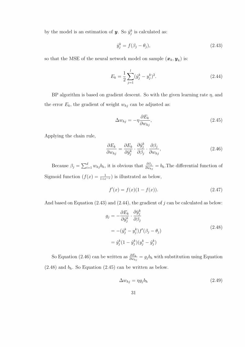
by the model is an estimation of y . So ykj is calculated as:

ykj = f(βj − θj), (2.43)

so that the MSE of the neural network model on sample (x k,yk) is:

Ek =1

2

l∑j=1

(ykj − ykj )2. (2.44)

BP algorithm is based on gradient descent. So with the given learning rate η, and

the error Ek, the gradient of weight whj can be adjusted as:

∆whj = −η ∂Ek∂whj

, (2.45)

Applying the chain rule,

∂Ek∂whj

=∂Ek∂ykj·∂ykj∂βj· ∂βj∂whj

, (2.46)

Because βj =∑d

i=1whjbh, it is obvious that∂βj∂whj

= bh.The differential function of

Sigmoid function (f(x) = 11+e−x ) is illustrated as below,

f ′(x) = f(x)(1− f(x)). (2.47)

And based on Equation (2.43) and (2.44), the gradient of j can be calculated as below:

gj = −∂Ek∂ykj·∂ykj∂βj

= −(ykj − ykj )f ′(βj − θj)

= ykj (1− ykj )(ykj − ykj )

(2.48)

So Equation (2.46) can be written as ∂Ek

∂whj= gjbh with substitution using Equation

(2.48) and bh. So Equation (2.45) can be written as below.

∆whj = ηgjbh (2.49)

31

Similarly, the other parameters in the specific neural network can be calculated,

∆θj = −ηgj,

∆vih = ηehxi,

∆γh = −ηeh,

where eh = −∂Ek∂bh· ∂bh∂αh

= −l∑

j=1

∂Ek∂βj· ∂βj∂bh

f ′(αh − γh)

=l∑

j=1

whjgjf′(αh − γh)

= bh(1− bh)l∑

j=1

whjgj.

(2.50)

The psuedo code below shows how the BP algorithm works:

Algorithm 2 Backpropagation Algorithm.Input:Training Dataset D = {(x 1,y1), (x 2,y2), · · · , (xm,ym)};Learning rate ηProcedure:

1: Initialize all the weights and threshold in (0, 1)2: repeat3: for all (x k,yk) ∈ D do4: Calculate yk by Equation (2.43) and current weights and thresholds.5: Calculate gj by Equation (2.48)6: Calculate eh by Equation (2.50)7: Update whj, vih, θj, γh by Equation (2.50)8: end for9: until The training error reaches the threshold, or the iteration reaches the thresh-

old.

Output:A multi-layer feedforward neural network with trained weights and thresholds.

The BP algorithm makes training multi-layer neural networks become possible.

32

Deep neural networks (DNNs), or neural networks with multiple hidden layers, have

been introduced in [17]. The major difference between DNNs and conventional arti-

ficial neural networks is the number of hidden layers. Typically, an artificial neural

network usually has three layers (the input layer, the hidden layer, and the output

layer), and is trained to be optimized for a specific task. Differently, DNNs have more

layers, and each layer in a DNN produces a representation of the patterns based on

the input data from the previous layer [17]. Recent research shows DNNs have been

applied to speech recognition, computer vision, and clinical data research [16]. The

following parts show some representative models based on DNNs.

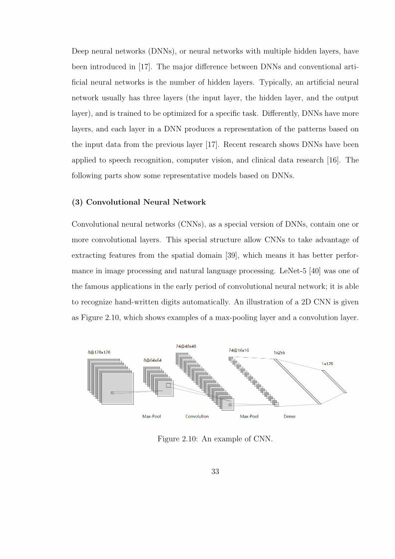
(3) Convolutional Neural Network

Convolutional neural networks (CNNs), as a special version of DNNs, contain one or

more convolutional layers. This special structure allow CNNs to take advantage of

extracting features from the spatial domain [39], which means it has better perfor-

mance in image processing and natural language processing. LeNet-5 [40] was one of

the famous applications in the early period of convolutional neural network; it is able

to recognize hand-written digits automatically. An illustration of a 2D CNN is given

as Figure 2.10, which shows examples of a max-pooling layer and a convolution layer.

Figure 2.10: An example of CNN.

33

A convolution layer usually has a convolution kernel, which slides the whole input

data in a specific order (usually from left to right (1D convolution), or from left top to

right bottom (2D convolution)) and extracts the relationships in the spatial domain.

Maxpooling layer is a special layer that outputs the maximum of the values in the

adjacent range of a specific data point.

Convolutional neural networks are widely applied on clinical image recognition.

Cirean et al. applied the convolutional neural network with max pooling layer on

breast cancer histology image data in order to detect mitosis, and won the ICPR

2012 mitosis detection competition [41]. Shen et al. proposed multi-scale convolu-

tional neural networks to automatically classify malignant and benign nodules from

computed tomography screening data without additional procedure of nodule seg-

mentation [42]. Esteva et al. trained a single CNN to classify skin cancer by using

disease-labeled images as input data [43].

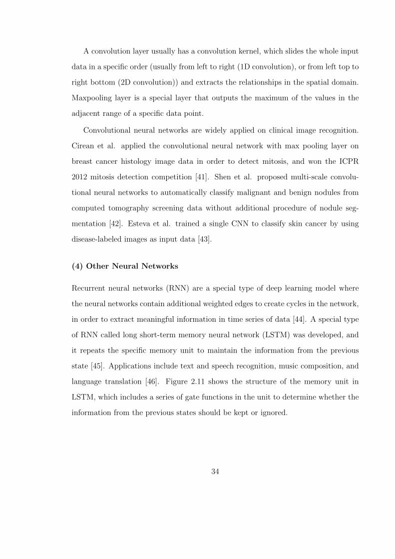
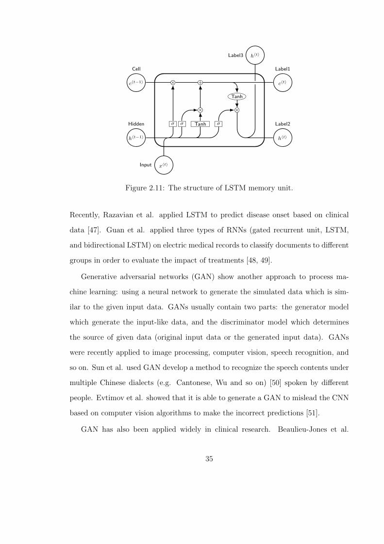
(4) Other Neural Networks

Recurrent neural networks (RNN) are a special type of deep learning model where

the neural networks contain additional weighted edges to create cycles in the network,

in order to extract meaningful information in time series of data [44]. A special type

of RNN called long short-term memory neural network (LSTM) was developed, and

it repeats the specific memory unit to maintain the information from the previous

state [45]. Applications include text and speech recognition, music composition, and

language translation [46]. Figure 2.11 shows the structure of the memory unit in

LSTM, which includes a series of gate functions in the unit to determine whether the

information from the previous states should be kept or ignored.

34

σ σ Tanh σ

× +

× ×

Tanh

c〈t−1〉

Cell

h〈t−1〉

Hidden

x〈t〉Input

c〈t〉

Label1

h〈t〉

Label2

h〈t〉Label3

Figure 2.11: The structure of LSTM memory unit.

Recently, Razavian et al. applied LSTM to predict disease onset based on clinical

data [47]. Guan et al. applied three types of RNNs (gated recurrent unit, LSTM,

and bidirectional LSTM) on electric medical records to classify documents to different

groups in order to evaluate the impact of treatments [48, 49].

Generative adversarial networks (GAN) show another approach to process ma-

chine learning: using a neural network to generate the simulated data which is sim-

ilar to the given input data. GANs usually contain two parts: the generator model

which generate the input-like data, and the discriminator model which determines

the source of given data (original input data or the generated input data). GANs

were recently applied to image processing, computer vision, speech recognition, and

so on. Sun et al. used GAN develop a method to recognize the speech contents under

multiple Chinese dialects (e.g. Cantonese, Wu and so on) [50] spoken by different

people. Evtimov et al. showed that it is able to generate a GAN to mislead the CNN

based on computer vision algorithms to make the incorrect predictions [51].

GAN has also been applied widely in clinical research. Beaulieu-Jones et al.

35

trained pairs of neural networks to generate simulated data from actual data, which

provided a method to share the simulated patients’ data while preserving their privacy

[52]. Shin et al. used GAN to generate synthetic abnormal MRI images with brain

tumors from public databases in order to increase the diversity of clinical MRI image

data [53]. Rezaei et al. applied GAN on generating segmentation label maps for

images of brain lesions [54].

(5) Platforms Related to Neural Networks

Neural network models with multi-neuron architecture are computationally intensive

but can be computed using parallel algorithms. To carry out these calculations, highly

parallelization-optimized hardware and software tools are strongly needed. A high

performance GPU with multicores and shareable large-capacity cache is needed to

accelerate the training process [55]. Multiple software platforms and tools for working

with and parallelizing neural networks have been developed, such as CUDA [32],

Tensorflow [56], and Keras [57]. The most common languages in machine learning,

especially for neural networks for academic research use, are Python and R, which

are easy to use and have a large number of relevant packages and resources.

In 2018, Nvidia developed the Volta GPU microarchitecture and introduced a

new specialized hardware unit called Tensor Core that is able to perform one matrix-

multiply-and-accumulate operation on 4× 4 matrices in a single clock cycle [56]. The

Tensor Cores are designed to make a tradeoff between the calculation precision and

the time efficiency, as mixed datatypes are used during the calculations, like half

precision float (float 16) and full precision float (float 32) [58]. Research shows that

NVIDIA Tensor Cores can strongly accelerate high performance computing through

efficient matrix multiplications with acceptable loss of calculation precision, , which

can be exploited in training deep learning models and related activities [59].

36

2.2 Unsupervised Learning

Unsupervised learning is used when the dataset is not labelled . In general, unsuper-

vised learning attempts to find the implicit relations between data, in order to extract

meaningful information from the data. Two examples are reducing the dimension of

the data (e.g., PCA) and performing clustering (e.g., K-means).

Principle components analysis (PCA) is a common unsupervised learning method

for dimensional reduction. It represents the original input feature set (annotated as

X = {x 1,x 2, · · · ,xm}) by generating principle components X ′ = {x ′1,x ′2, · · · ,x ′k},

k < m, which are in the lower dimension using singular vector decomposition. The

pseudo code below describes how PCA works.

Algorithm 3 Principle Components Analysis.Input:The dataset with m input features X = {x 1,x 2, · · · ,xm}The number k of principle components to be generated.Procedure:

1: x i ← x i − 1m

∑mj=1 x j . Centralizing x i

2: Calculate the covariance matrix XXT for X.3: v ,S ← SVD(XXT ) . Singular values v = {v1, v2, · · · , vm} and singular vectors

S = {S 1,S 2, · · · ,Sm}4: Select k singular vectors S with the k largest singular values.5: Put the selected singular vectors S in a new set X ′

Output:Principle components X ’

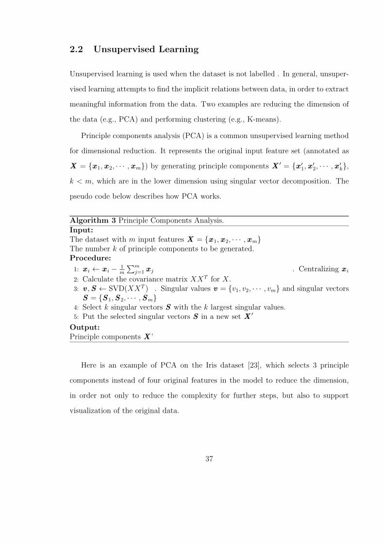
Here is an example of PCA on the Iris dataset [23], which selects 3 principle

components instead of four original features in the model to reduce the dimension,

in order not only to reduce the complexity for further steps, but also to support

visualization of the original data.

37

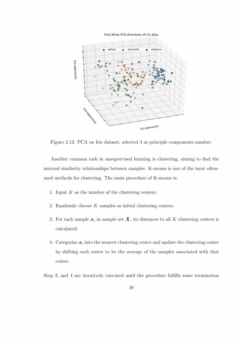
Figure 2.12: PCA on Iris dataset, selected 3 as principle components number.

Another common task in unsupervised learning is clustering, aiming to find the

internal similarity relationships between samples. K-means is one of the most often-

used methods for clustering. The main procedure of K-means is:

1. Input K as the number of the clustering centers;

2. Randomly choose K samples as initial clustering centers;

3. For each sample x i in sample set X , its distances to all K clustering centers is

calculated;

4. Categorize x i into the nearest clustering center and update the clustering center

by shifting each center to be the average of the samples associated with that

center.

Step 3, and 4 are iteratively executed until the procedure fulfills some termination

38

condition(s), such as all samples are clustered, no clustering center is changing, and/or

the MSE of all samples reaches a minimum.

Because of its efficiency and simplicity, K-Means clustering has been used in clin-

ical data research for unsupervised learning. Haldar et al. used K-means clustering

in three independent asthma datasets of patients’ records, to identify asthma phe-

notypes for making different treatment decisions [60]. Tothill et al. attempted to

identify novel molecular subtypes of ovarian cancer by using K-means and to evaluate

the patients survival within k-means groups by Cox proportional hazards models [61].

However, the main drawback of K-means is the number of clustering centers K

should be estimated and specified in advance, but it is not straightforward to estimate

a proper K. Also, instead of clustering samples by generating borders, K-means clus-

ters the samples by optimizing the center of clustering, which often leads to incorrectly

clustering samples [17].

2.3 Reinforcement Learning

In reinforcement learning, the training target is to develop a model (agent) which is

able to improve its performance by interacting with the environment [62], as Figure

2.13 illustrates. A so-called reward signal is generated to indicate how well the model

is interacting with the environment as defined by a reward function, which is different

from the value or label used in supervised learning.

Figure 2.13: Reinforcement learning structure.

39

During the training process of reinforcement learning, the agent attempts to learn

a policy π, and using π generates the action a = π(x) based on the environment state

x, which brings the optimal reward. One famous example of reinforcement learning

is AlphaGo, a go (a kind of board game) AI developed by Google Deepmind [63].

By using reinforcement learning to train itself, AlphaGo defeats some top go players

around the world, including Ke Jie and Lee Sedol, which shows the strong power

of reinforcement learning. Moreover, reinforcement learning has a broad future with

potential uses in industrial manufacturing, game AI designing, and even tuning the

hyperparameters for other machine learning models [64].

40

Chapter 3: Ensemble Methods and Cascade Forest

3.1 Basic Theory of Ensemble Methods

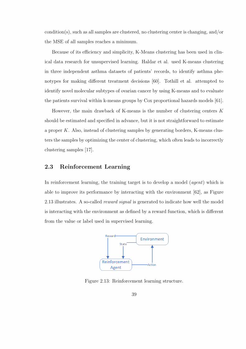
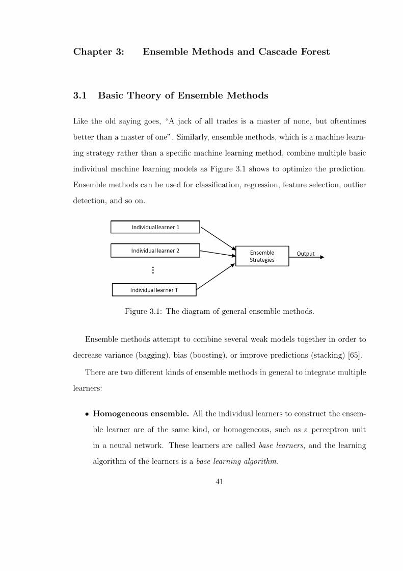
Like the old saying goes, “A jack of all trades is a master of none, but oftentimes

better than a master of one”. Similarly, ensemble methods, which is a machine learn-

ing strategy rather than a specific machine learning method, combine multiple basic

individual machine learning models as Figure 3.1 shows to optimize the prediction.

Ensemble methods can be used for classification, regression, feature selection, outlier

detection, and so on.

Figure 3.1: The diagram of general ensemble methods.

Ensemble methods attempt to combine several weak models together in order to

decrease variance (bagging), bias (boosting), or improve predictions (stacking) [65].

There are two different kinds of ensemble methods in general to integrate multiple

learners:

• Homogeneous ensemble. All the individual learners to construct the ensem-

ble learner are of the same kind, or homogeneous, such as a perceptron unit

in a neural network. These learners are called base learners, and the learning

algorithm of the learners is a base learning algorithm.

41

• Heterogeneous ensemble. Some individual learners are not the same, or

heterogeneous. The learners in heterogeneous ensemble are called as component

learners, which are generated from different machine learning algorithms. For

example, considering a specific classification problem, different models including

SVM, logistic regression, and neural network are applied on the training data.

From the point of base learners’ organization, ensemble methods can be also di-

vided into 2 groups:

• Sequential ensemble methods. Each base learner is generated sequentially

to exploit the dependence between the base learners. Boosting [66] is one of the

most representative examples of sequential ensemble methods.

• Parallel ensemble methods. Each base learner is generated in parallel to

exploit the independence between the base learners in order to reduce the error.

One of the most popular parallel ensemble methods is bagging [67].

3.2 Ensemble Strategies

Ensemble strategies integrate the outputs from individual learners. Averaging, voting,

and stacking are the three typical ensemble strategies.

Assume the ensemble modelH contains T base learners, annotated as {h1, h2, · · · , hT}.

The output for each base learner is hi(x ), when x is the given input. The following

parts illustrates averaging, voting, and stacking of integrating the outputs.

For regression tasks, the common strategy is averaging. Averaging is described as

Equation (3.1), where wt represents the weight for learner ht(·).

42

H(x ) =1

T

T∑t=1

wtht(x )

T∑t=1

wt = 1

(3.1)

This equation describes simple averaging when all of the base learners have the same

weight. Otherwise, if the weights are different, it is called as weighted averaging.

Different from averaging, voting is a method which performs better on classifica-

tion tasks [65]. For the same sample x i, the voting strategy lets the ensemble model

generate the output on the basis of the majority of individual learner ht.

Stacking is a technique for ensemble learning which combines multiple learners via

an integrated learner, described as meta-learner (meta-classifier or meta-regressor).

The individual learners in base level are trained with all of the input training data.

Then the meta-model is trained on both of the label from training data Y and the

outputs of the base level models as features z , to generate the output H. The basic

algorithm of stacking is illustrated as below:

43

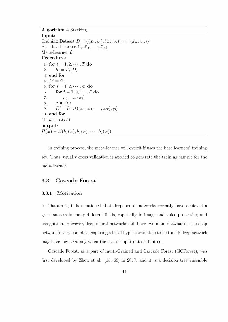
Algorithm 4 Stacking.Input:Training Dataset D = {(x 1, y1), (x 2, y2), · · · , (xm, ym)};Base level learner L1,L2, · · · ,LT ;Meta-Learner LProcedure:

1: for t = 1, 2, · · · , T do2: ht = Lt(D)3: end for4: D′ = ∅5: for i = 1, 2, · · · ,m do6: for t = 1, 2, · · · , T do7: zit = ht(x i)8: end for9: D′ = D′ ∪ ((zi1, zi2, · · · , ziT ), yi)

10: end for11: h′ = L(D′)

output:H(x ) = h′(h1(x ), h1(x ), · · · , h1(x ))

In training process, the meta-learner will overfit if uses the base learners’ training

set. Thus, usually cross validation is applied to generate the training sample for the

meta-learner.

3.3 Cascade Forest

3.3.1 Motivation

In Chapter 2, it is mentioned that deep neural networks recently have achieved a

great success in many different fields, especially in image and voice processing and

recognition. However, deep neural networks still have two main drawbacks: the deep

network is very complex, requiring a lot of hyperparameters to be tuned; deep network

may have low accuracy when the size of input data is limited.

Cascade Forest, as a part of multi-Grained and Cascade Forest (GCForest), was

first developed by Zhou et al. [15, 68] in 2017, and it is a decision tree ensemble

44

method. Inspired by the layer structure of deep neural network, cascade forest also

has a typical layer-by-layer structure.

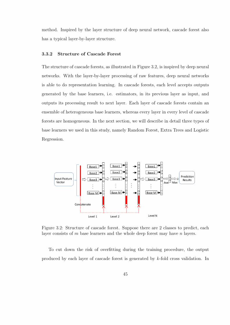
3.3.2 Structure of Cascade Forest

The structure of cascade forests, as illustrated in Figure 3.2, is inspired by deep neural

networks. With the layer-by-layer processing of raw features, deep neural networks

is able to do representation learning. In cascade forests, each level accepts outputs

generated by the base learners, i.e. estimators, in its previous layer as input, and

outputs its processing result to next layer. Each layer of cascade forests contain an

ensemble of heterogeneous base learners, whereas every layer in every level of cascade

forests are homogeneous. In the next section, we will describe in detail three types of

base learners we used in this study, namely Random Forest, Extra Trees and Logistic

Regression.

Figure 3.2: Structure of cascade forest. Suppose there are 2 classes to predict, eachlayer consists of m base learners and the whole deep forest may have n layers.

To cut down the risk of overfitting during the training procedure, the output

produced by each layer of cascade forest is generated by k -fold cross validation. In

45

detail, each specific sample from the training set will be used as training data for

k− 1 times to generate k− 1 outputs. Then the output for this layer is generated by

the average of the k−1 outputs. Before generating new layer, the performance of the

whole cascade forest can be evaluated on the validation set. If the performance does

not gain significantly, the training procedure will be terminated, which means the

number of layers in cascade forest is automatically decided. In contrast to most deep

neural networks whose model complexity is stable and set by hyperparameters, this

feature of cascade forest shows the ability to terminate the training process adaptively,

which enables this ensemble method to decide its model complexity and let GCForest

be able to process both small and large scales of training data [15].

Since GCForest was developed in 2017, research [68] about the applications and

improvements of deep forest model have been popular. Utkin et al. attempted to

weight the outputs from base learners per layer and get the weighted average result

as output for this layer. These weights are able to be trained, in order to improve the

accuracy of cascade forest and converge the model rapidly [69].

Some recent works about cancer clinical data research based on deep forest model

are listed below. Guo et al. developed BCDForest based on modifying GCforest [70],

to address cancer subtype classification on small-scale genomic datasets in 2018. By

adding boosting to the standard cascade forest model, they used the modified model

BCDForest to analyze the genomic data from TCGA, to distinguish 11 different types

of cancer, including breast cancer, lung cancer, and so on. Su et al. proposed Deep-

Resp-Forest, based on the GCForest, to evaluate the response of anti-cancer drugs by

training the proposed model to classify the labeled data as “sensitive” or “resistant”

[71].

46

3.3.3 Base Learners of Cascade Forest

In this thesis, we choose random forest, extra trees, and logistic regression as indi-

vidual learners because these methods need less time and fewer hyperparameters as

compared to neural networks and SVM. Also, more heterogeneous individual learners

in the ensemble cascade forest model improve the diversity of whole model, which

helps make predictions more accurately [68]. The following parts describe these three

base learners briefly.

(1) Random Forest

Just like the relationship between trees and forests in the real world, random forests

(RF) contain a set of decision trees [67]. Specifically, random forests use Bootstrap

AGGregation (Bagging) to sample data, and use the results of a set of decision trees

to generate the output. Bagging uses bootstrap sampling to get the subsets of features

for training the base learners. Then the subsets, i.e. the set of samples, of the original

samples are generated. With these subsets of samples, each decision tree is generated

as a base learner from the different sampling set. To aggregate the outputs from the

base learners, bagging uses the majority of voting the outputs for classification, and

the average of the outputs for regression. The pseudo code of bagging is given as

below:

47

Algorithm 5 Bagging Algorithm.Input:Training Dataset D = {(x 1, y1), (x 2, y2), · · · , (xm, ym)};Base decision method L;Maximum training iteration TProcedure:

1: for t = 1, 2, · · · , T do2: ht = L(D,Dbs) . Dbs ⊂ D is generated from bootstrap sampling.3: end for

output:H(x ) = argmax

y∈Y

∑Tt=1 I(ht(x ) = y)

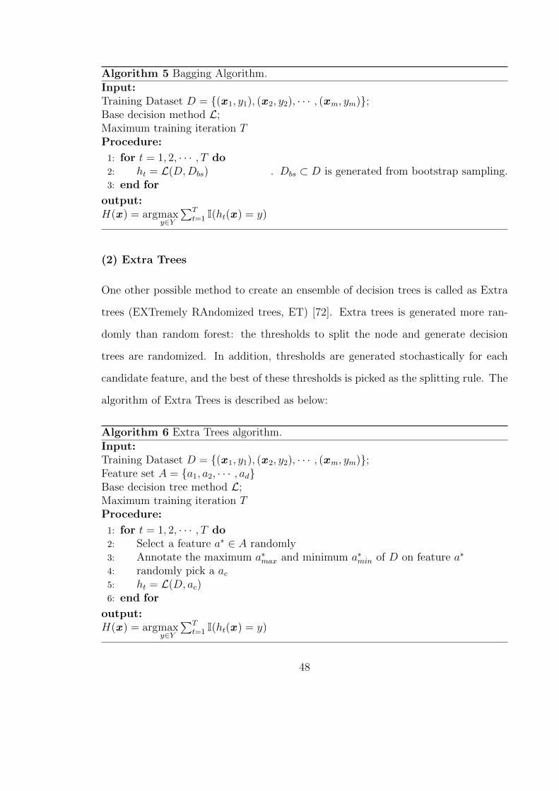
(2) Extra Trees

One other possible method to create an ensemble of decision trees is called as Extra

trees (EXTremely RAndomized trees, ET) [72]. Extra trees is generated more ran-

domly than random forest: the thresholds to split the node and generate decision

trees are randomized. In addition, thresholds are generated stochastically for each

candidate feature, and the best of these thresholds is picked as the splitting rule. The

algorithm of Extra Trees is described as below:

Algorithm 6 Extra Trees algorithm.Input:Training Dataset D = {(x 1, y1), (x 2, y2), · · · , (xm, ym)};Feature set A = {a1, a2, · · · , ad}Base decision tree method L;Maximum training iteration TProcedure:

1: for t = 1, 2, · · · , T do2: Select a feature a∗ ∈ A randomly3: Annotate the maximum a∗max and minimum a∗min of D on feature a∗

4: randomly pick a ac5: ht = L(D, ac)6: end for

output:H(x ) = argmax

y∈Y

∑Tt=1 I(ht(x ) = y)

48

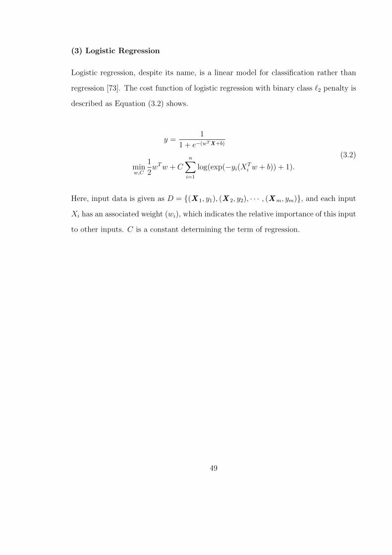
(3) Logistic Regression

Logistic regression, despite its name, is a linear model for classification rather than

regression [73]. The cost function of logistic regression with binary class `2 penalty is

described as Equation (3.2) shows.

y =1

1 + e−(wTX+b)

minw,C

1

2wTw + C

n∑i=1

log(exp(−yi(XTi w + b)) + 1).

(3.2)

Here, input data is given as D = {(X 1, y1), (X 2, y2), · · · , (Xm, ym)}, and each input

Xi has an associated weight (wi), which indicates the relative importance of this input

to other inputs. C is a constant determining the term of regression.

49

Chapter 4: Applying Cascade Forest on the SEER

Dataset for Survivability Prediction of Lung Cancer

This chapter focuses on applying the proposed cascade forest model described

in detail in Chapter 3 on the clinical data analysis, and making comparison with

conventional methods illustrated in Chapters 2 and 3. The following sections intro-

duce the classification of survivability data acquisition, data preprocessing, model

construction, model evaluation, and comparisons.

4.1 Data Acquisition and Preprocessing

4.1.1 SEER Dataset

In this thesis, the clinical data used is “Incidence - SEER 18 Regs Research Data

+ Hurricane Katrina Impacted Louisiana Cases, Nov 2017 Sub (1973-2015 varying)”

from the Surveillance, Epidemiology, and End Results Program (SEER) [7]. This

database covers approximately 27.8% of the U.S. population (based on 2010 census)

and contains records for 10,050,814 tumors in total [4]. All tumors recorded in SEER

are categorized into 22 main classes. Lung cancer is classified in the main class

“Respiratory System” and the branch “Lung and Bronchus”. In this database, a

clinical record for one specific patient’s case, i.e. record of tumor, has 191 features

and this record is encoded in a single row. A brief description of all features from

SEER is listed in Appendix B. [74]. These features can be categorized as Table 4.1.1

shows.

50

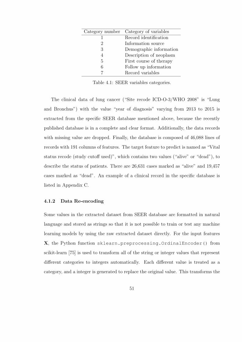
Category number Category of variables1 Record identification2 Information source3 Demographic information4 Description of neoplasm5 First course of therapy6 Follow up information7 Record variables

Table 4.1: SEER variables categories.

The clinical data of lung cancer (“Site recode ICD-O-3/WHO 2008” is “Lung

and Bronchus”) with the value “year of diagnosis” varying from 2013 to 2015 is

extracted from the specific SEER database mentioned above, because the recently

published database is in a complete and clear format. Additionally, the data records

with missing value are dropped. Finally, the database is composed of 46,088 lines of

records with 191 columns of features. The target feature to predict is named as “Vital

status recode (study cutoff used)”, which contains two values (“alive” or “dead”), to

describe the status of patients. There are 26,631 cases marked as “alive” and 19,457

cases marked as “dead”. An example of a clinical record in the specific database is

listed in Appendix C.

4.1.2 Data Re-encoding

Some values in the extracted dataset from SEER database are formatted in natural

language and stored as strings so that it is not possible to train or test any machine

learning models by using the raw extracted dataset directly. For the input features

X, the Python function sklearn.preprocessing.OrdinalEncoder() from

scikit-learn [75] is used to transform all of the string or integer values that represent

different categories to integers automatically. Each different value is treated as a

category, and a integer is generated to replace the original value. This transforms the

51

original input data to a single column of integers (0 to number of categories - 1) for

each feature. For the target feature Y, all records labeled as “alive” are re-encoded

as “1”, while the others are re-encoded as “0”.

4.1.3 Dimensional Reduction

Dimensional reduction is applied on the extracted SEER dataset in order to reduce

the complexity of the machine learning model. First of all, because the type of cancer

selected is “Lung and Bronchus”, some of the features are not proper for lung cancer,

and should be eliminated from the feature set. For example, features like “Histology

recode - Brain groupings”, “Breast - Adjusted AJCC 6th T (1988+)”, “Breast -

Adjusted AJCC 6th N (1988+)”, and “Breast - Adjusted AJCC 6th M (1988+)”

are designed for tumors on different sites (brain or breast) rather than lung, which

are not related to lung cancer. Second, features which have high correlations with

the target feature “Vital status recode (study cutoff used)” are dropped. Also, some

columns of the extracted data contain just one value, which is not appropriate for

training the model. Thus 113 features are dropped due to the reasons described

above. Additionally, “Patient ID” in SEER database is only used to distinguish

patients, which has little significance to the prediction result, so that it was dropped

manually. As a result, our extracted dataset contained 77 features.

To compare our results with recent studies [11] [76] [77], we manually generated a

subset with 11 features listed in Table 4.2 that were selected for further analysis on

Lung cancer data from the SEER database. Since the SEER database was updated

after the prior studies in content and feature names, we attempted to reproduce the

features set and used the updated SEER database.

52

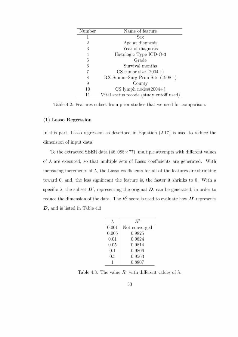
Number Name of feature1 Sex2 Age at diagnosis3 Year of diagnosis4 Histologic Type ICD-O-35 Grade6 Survival months7 CS tumor size (2004+)8 RX Summ–Surg Prim Site (1998+)9 County10 CS lymph nodes(2004+)11 Vital status recode (study cutoff used)

Table 4.2: Features subset from prior studies that we used for comparison.

(1) Lasso Regression

In this part, Lasso regression as described in Equation (2.17) is used to reduce the

dimension of input data.

To the extracted SEER data (46, 088×77), multiple attempts with different values

of λ are executed, so that multiple sets of Lasso coefficients are generated. With

increasing increments of λ, the Lasso coefficients for all of the features are shrinking

toward 0, and, the less significant the feature is, the faster it shrinks to 0. With a

specific λ, the subset D ′, representing the original D , can be generated, in order to

reduce the dimension of the data. The R2 score is used to evaluate how D ′ represents

D , and is listed in Table 4.3

λ R2

0.001 Not converged0.005 0.98250.01 0.98240.05 0.98140.1 0.98060.5 0.95631 0.8807

Table 4.3: The value R2 with different values of λ.

53

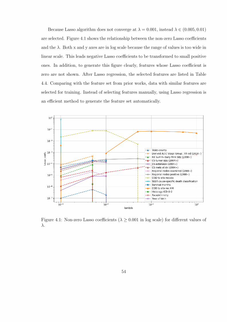
Because Lasso algorithm does not converge at λ = 0.001, instead λ ∈ (0.005, 0.01)

are selected. Figure 4.1 shows the relationship between the non-zero Lasso coefficients

and the λ. Both x and y axes are in log scale because the range of values is too wide in

linear scale. This leads negative Lasso coefficients to be transformed to small positive

ones. In addition, to generate this figure clearly, features whose Lasso coefficient is

zero are not shown. After Lasso regression, the selected features are listed in Table

4.4. Comparing with the feature set from prior works, data with similar features are

selected for training. Instead of selecting features manually, using Lasso regression is

an efficient method to generate the feature set automatically.

Figure 4.1: Non-zero Lasso coefficients (λ ≥ 0.001 in log scale) for different values ofλ.

54

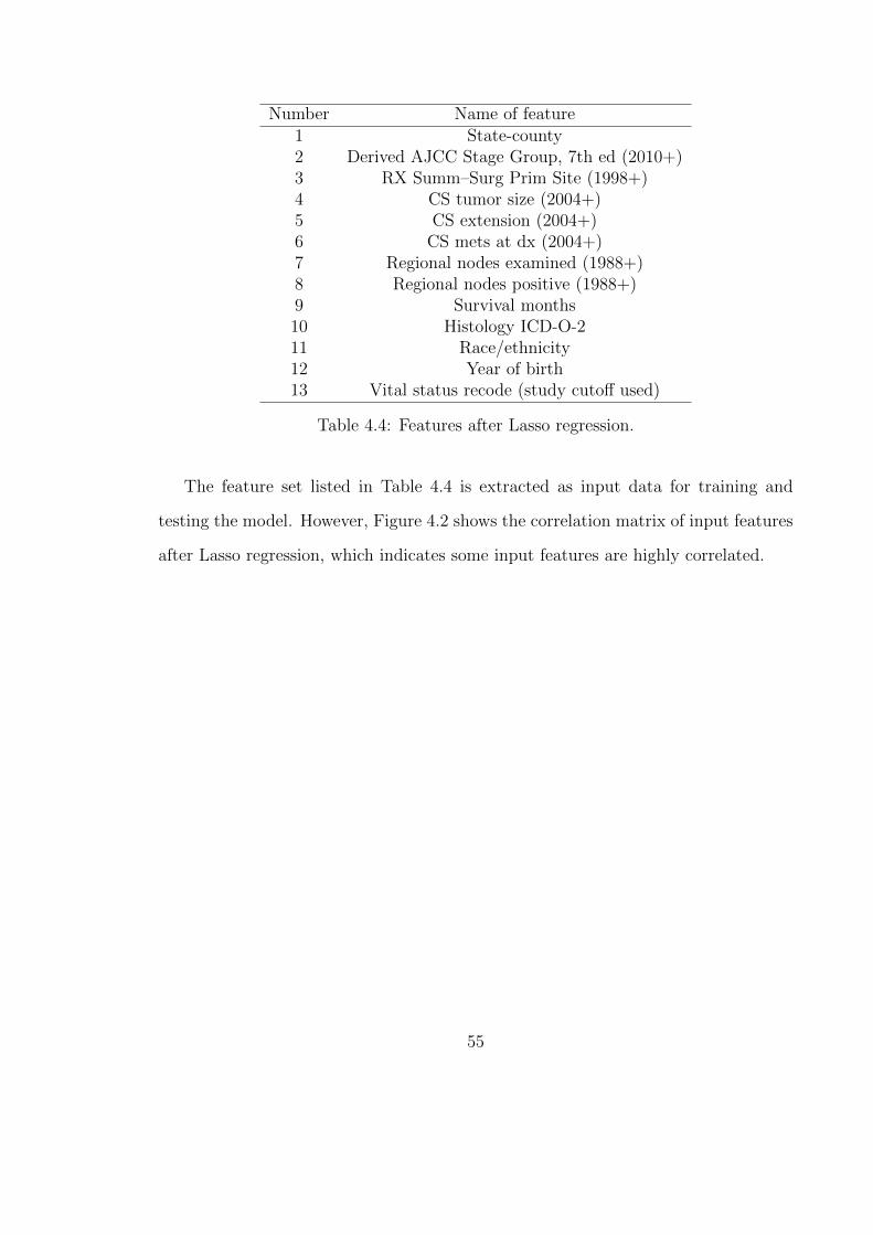
Number Name of feature1 State-county2 Derived AJCC Stage Group, 7th ed (2010+)3 RX Summ–Surg Prim Site (1998+)4 CS tumor size (2004+)5 CS extension (2004+)6 CS mets at dx (2004+)7 Regional nodes examined (1988+)8 Regional nodes positive (1988+)9 Survival months10 Histology ICD-O-211 Race/ethnicity12 Year of birth13 Vital status recode (study cutoff used)

Table 4.4: Features after Lasso regression.

The feature set listed in Table 4.4 is extracted as input data for training and

testing the model. However, Figure 4.2 shows the correlation matrix of input features

after Lasso regression, which indicates some input features are highly correlated.

55

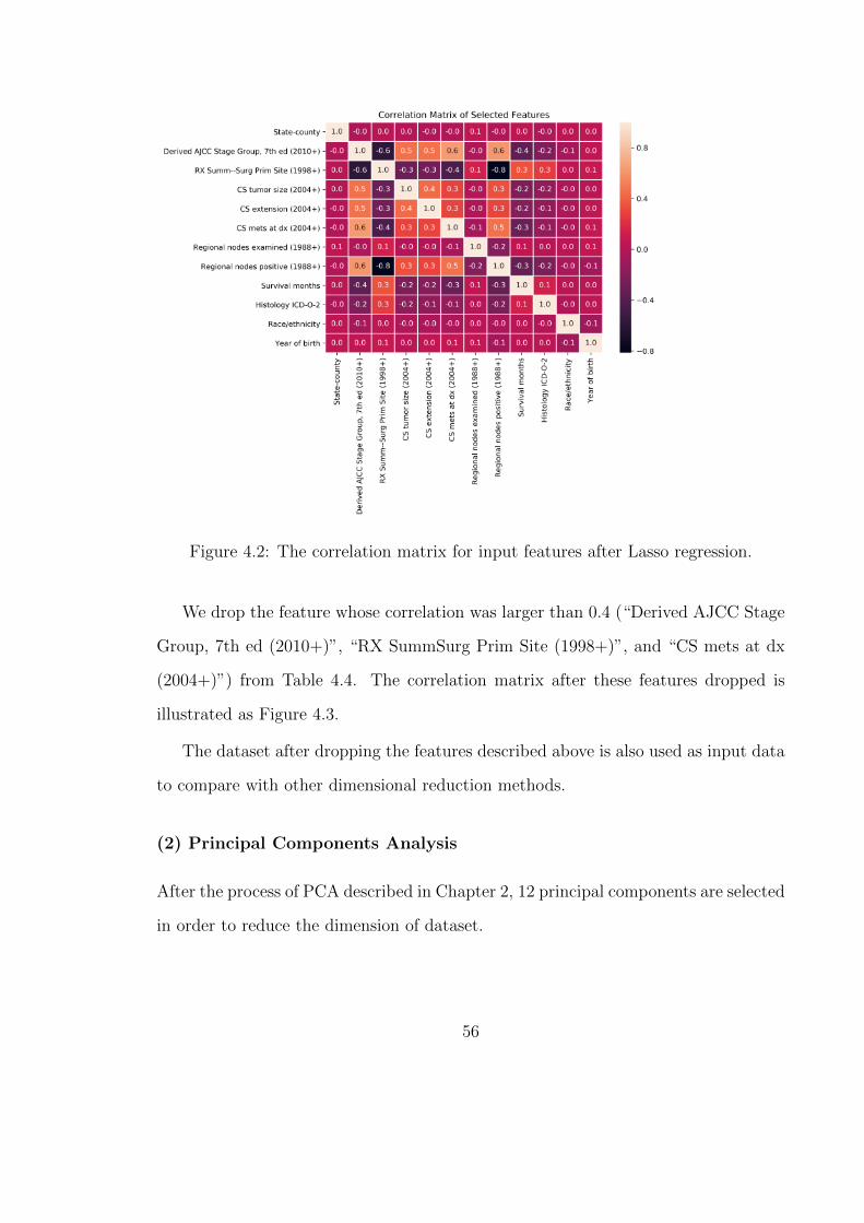
Figure 4.2: The correlation matrix for input features after Lasso regression.

We drop the feature whose correlation was larger than 0.4 (“Derived AJCC Stage

Group, 7th ed (2010+)”, “RX SummSurg Prim Site (1998+)”, and “CS mets at dx

(2004+)”) from Table 4.4. The correlation matrix after these features dropped is

illustrated as Figure 4.3.

The dataset after dropping the features described above is also used as input data

to compare with other dimensional reduction methods.

(2) Principal Components Analysis

After the process of PCA described in Chapter 2, 12 principal components are selected

in order to reduce the dimension of dataset.

56

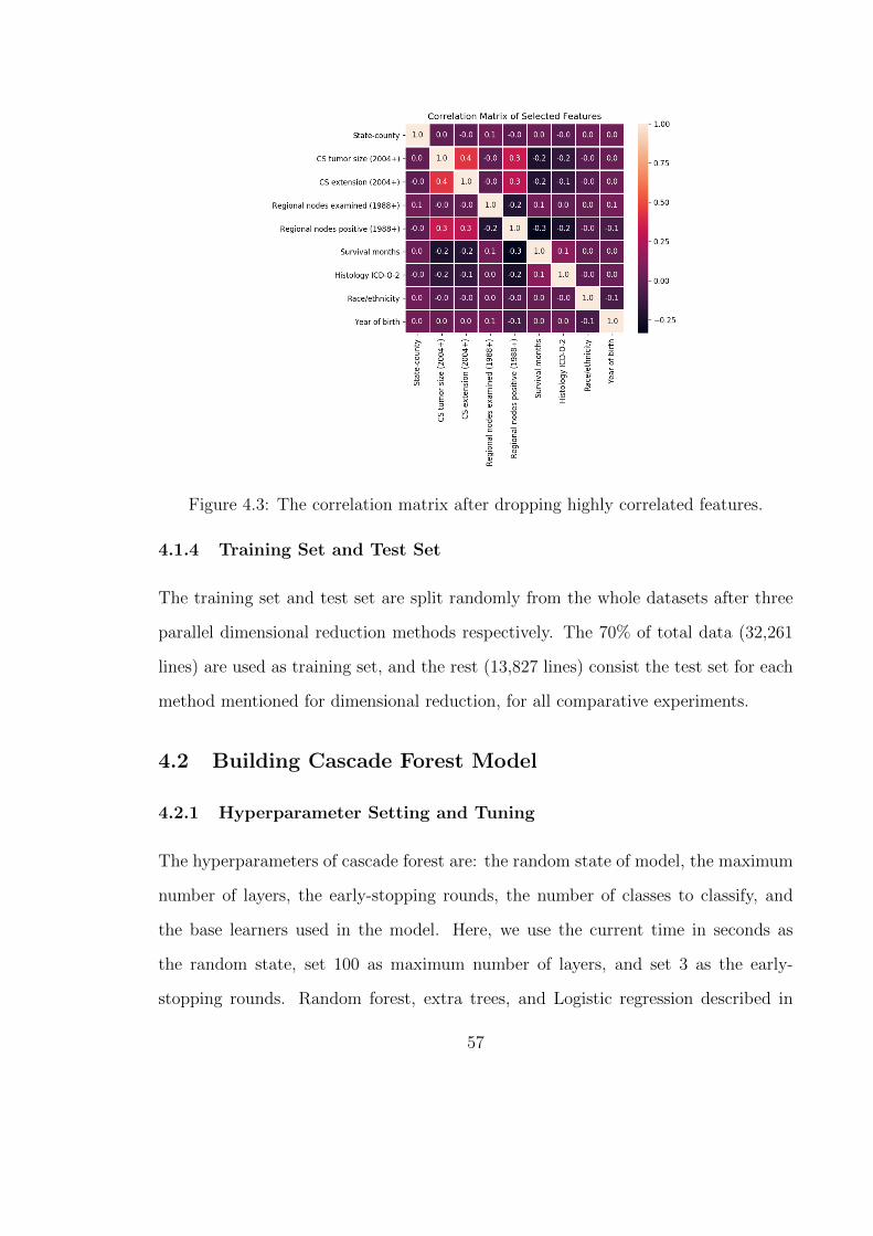
Figure 4.3: The correlation matrix after dropping highly correlated features.

4.1.4 Training Set and Test Set

The training set and test set are split randomly from the whole datasets after three

parallel dimensional reduction methods respectively. The 70% of total data (32,261

lines) are used as training set, and the rest (13,827 lines) consist the test set for each

method mentioned for dimensional reduction, for all comparative experiments.

4.2 Building Cascade Forest Model

4.2.1 Hyperparameter Setting and Tuning

The hyperparameters of cascade forest are: the random state of model, the maximum

number of layers, the early-stopping rounds, the number of classes to classify, and

the base learners used in the model. Here, we use the current time in seconds as

the random state, set 100 as maximum number of layers, and set 3 as the early-

stopping rounds. Random forest, extra trees, and Logistic regression described in

57

Chapter 3 are used as base learners. From the experiments made in this thesis,

the hyperparameters for the cascade forest itself do not need to be tuned too much,

whereas the hyperparameters for base learners need to be well tuned. Instead of

tuning hyperparameters manually, we applied randomized grid search [78], which

automatically attempts the value of hyperparameters from a designed set randomly,

on three base learners of cascade forest to improve its performance.

The python code below shows the tuning process for random forest base learner

as an example:

param_dist_RF = {

"max_depth": [5, 10, 50, 100, None],

"n_estimators": sp_randint(1, 11),

"criterion": ["gini", "entropy"]

}

n_iter = 20

random_RF = RandomizedSearchCV(RF,

param_distributions=param_dist_RF,

n_iter=n_iter, cv=5)

Here in the code, the hyperparameters for random forest listed in “param dist RF” in-

dicate the shape of the random forest, using bootstrap or not, and using which kind of

splitting method for the decision tree in it. The function RandomizedSearchCV()

can automatically generate a number of parameter sets (here is 20), and measure the

performance using cross validation (here is a 5-fold cv).

Finally, the optimal hyperparameters for cascade forest’s base learners are gener-

ated, as python code below shows:

ca_config["estimators"].append({"n_folds": 5,

"type": "RandomForestClassifier",

"n_estimators": 10, "max_depth": None,

"criterion":"gini"})

ca_config["estimators"].append({"n_folds": 5,

"type": "ExtraTreesClassifier",

"n_estimators": 8, "max_depth": None,

"criterion":"gini"})

58

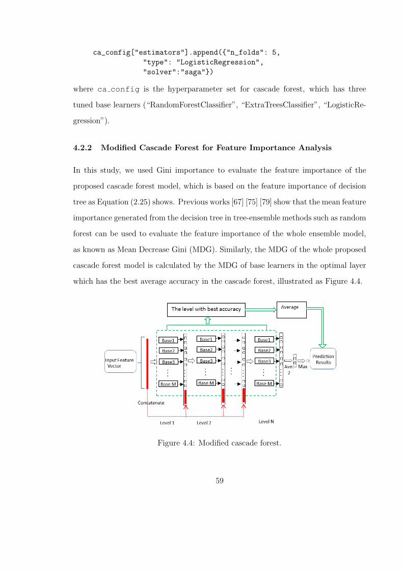
ca_config["estimators"].append({"n_folds": 5,

"type": "LogisticRegression",

"solver":"saga"})

where ca config is the hyperparameter set for cascade forest, which has three

tuned base learners (“RandomForestClassifier”, “ExtraTreesClassifier”, “LogisticRe-

gression”).

4.2.2 Modified Cascade Forest for Feature Importance Analysis

In this study, we used Gini importance to evaluate the feature importance of the

proposed cascade forest model, which is based on the feature importance of decision

tree as Equation (2.25) shows. Previous works [67] [75] [79] show that the mean feature

importance generated from the decision tree in tree-ensemble methods such as random

forest can be used to evaluate the feature importance of the whole ensemble model,

as known as Mean Decrease Gini (MDG). Similarly, the MDG of the whole proposed

cascade forest model is calculated by the MDG of base learners in the optimal layer

which has the best average accuracy in the cascade forest, illustrated as Figure 4.4.

Figure 4.4: Modified cascade forest.

59

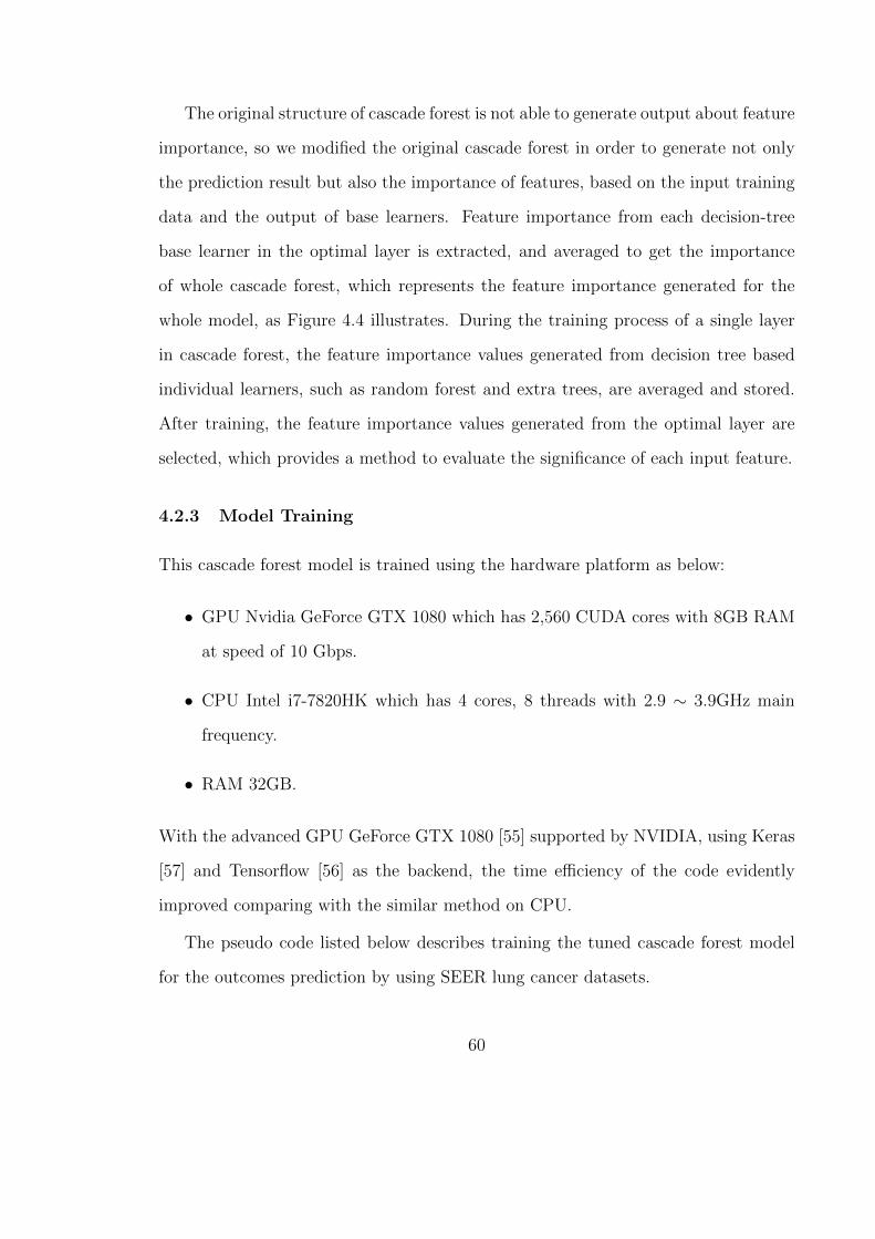
The original structure of cascade forest is not able to generate output about feature

importance, so we modified the original cascade forest in order to generate not only

the prediction result but also the importance of features, based on the input training

data and the output of base learners. Feature importance from each decision-tree

base learner in the optimal layer is extracted, and averaged to get the importance

of whole cascade forest, which represents the feature importance generated for the

whole model, as Figure 4.4 illustrates. During the training process of a single layer

in cascade forest, the feature importance values generated from decision tree based

individual learners, such as random forest and extra trees, are averaged and stored.

After training, the feature importance values generated from the optimal layer are

selected, which provides a method to evaluate the significance of each input feature.

4.2.3 Model Training

This cascade forest model is trained using the hardware platform as below:

• GPU Nvidia GeForce GTX 1080 which has 2,560 CUDA cores with 8GB RAM

at speed of 10 Gbps.

• CPU Intel i7-7820HK which has 4 cores, 8 threads with 2.9 ∼ 3.9GHz main

frequency.

• RAM 32GB.

With the advanced GPU GeForce GTX 1080 [55] supported by NVIDIA, using Keras

[57] and Tensorflow [56] as the backend, the time efficiency of the code evidently

improved comparing with the similar method on CPU.

The pseudo code listed below describes training the tuned cascade forest model

for the outcomes prediction by using SEER lung cancer datasets.

60

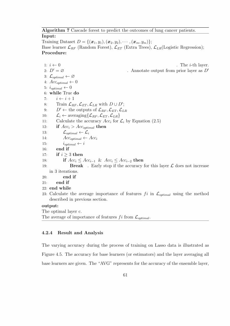
Algorithm 7 Cascade forest to predict the outcomes of lung cancer patients.Input:Training Dataset D = {(x 1, y1), (x 2, y2), · · · , (xm, ym)};Base learner LRF (Random Forest), LET (Extra Trees), LLR(Logistic Regression);Procedure:

1: i← 0 . The i-th layer.2: D′ = ∅ . Annotate output from prior layer as D′

3: Loptimal ← ∅4: Accoptimal ← 05: ioptimal ← 06: while True do7: i← i+ 18: Train LRF ,LET ,LLR with D ∪D′;9: D′ ← the outputs of LRF ,LET ,LLR

10: Li ← averaging{LRF ,LET ,LLR}11: Calculate the accuracy Acci for Li by Equation (2.5)12: if Acci > Accoptimal then13: Loptimal ← Li14: Accoptimal ← Acci15: ioptimal ← i16: end if17: if i ≥ 3 then18: if Acci ≤ Acci−1 & Acci ≤ Acci−2 then19: Break . Early stop if the accuracy for this layer L does not increase

in 3 iterations.20: end if21: end if22: end while23: Calculate the average importance of features fi in Loptimal using the method

described in previous section.

output:The optimal layer c.The average of importance of features fi from Loptimal.

4.2.4 Result and Analysis

The varying accuracy during the process of training on Lasso data is illustrated as

Figure 4.5. The accuracy for base learners (or estimators) and the layer averaging all

base learners are given. The “AVG” represents for the accuracy of the ensemble layer,

61

calculated by averaging the accuracy of base learners in this layer. From Figure 4.5,

the algorithm detected the averaging layer accuracy does not increase for generating

three layers after layer 6 was trained, so that it terminate the training process and

make an early stop.

Figure 4.5: Training accuracy of estimators in cascade forest, trained by Lasso data.

After training the cascade forest models, the test sets from the different datasets

are analyzed by the respective cascade forest models. As Table 4.5 shows, some

indicators listed below are used to evaluate the performance of cascade forest.

62

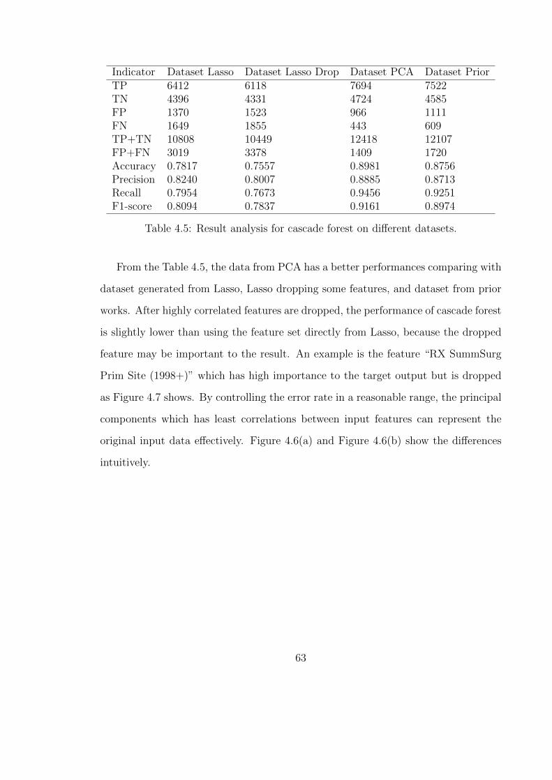
Indicator Dataset Lasso Dataset Lasso Drop Dataset PCA Dataset PriorTP 6412 6118 7694 7522TN 4396 4331 4724 4585FP 1370 1523 966 1111FN 1649 1855 443 609TP+TN 10808 10449 12418 12107FP+FN 3019 3378 1409 1720Accuracy 0.7817 0.7557 0.8981 0.8756Precision 0.8240 0.8007 0.8885 0.8713Recall 0.7954 0.7673 0.9456 0.9251F1-score 0.8094 0.7837 0.9161 0.8974

Table 4.5: Result analysis for cascade forest on different datasets.

From the Table 4.5, the data from PCA has a better performances comparing with

dataset generated from Lasso, Lasso dropping some features, and dataset from prior

works. After highly correlated features are dropped, the performance of cascade forest

is slightly lower than using the feature set directly from Lasso, because the dropped

feature may be important to the result. An example is the feature “RX SummSurg

Prim Site (1998+)” which has high importance to the target output but is dropped

as Figure 4.7 shows. By controlling the error rate in a reasonable range, the principal

components which has least correlations between input features can represent the

original input data effectively. Figure 4.6(a) and Figure 4.6(b) show the differences

intuitively.

63

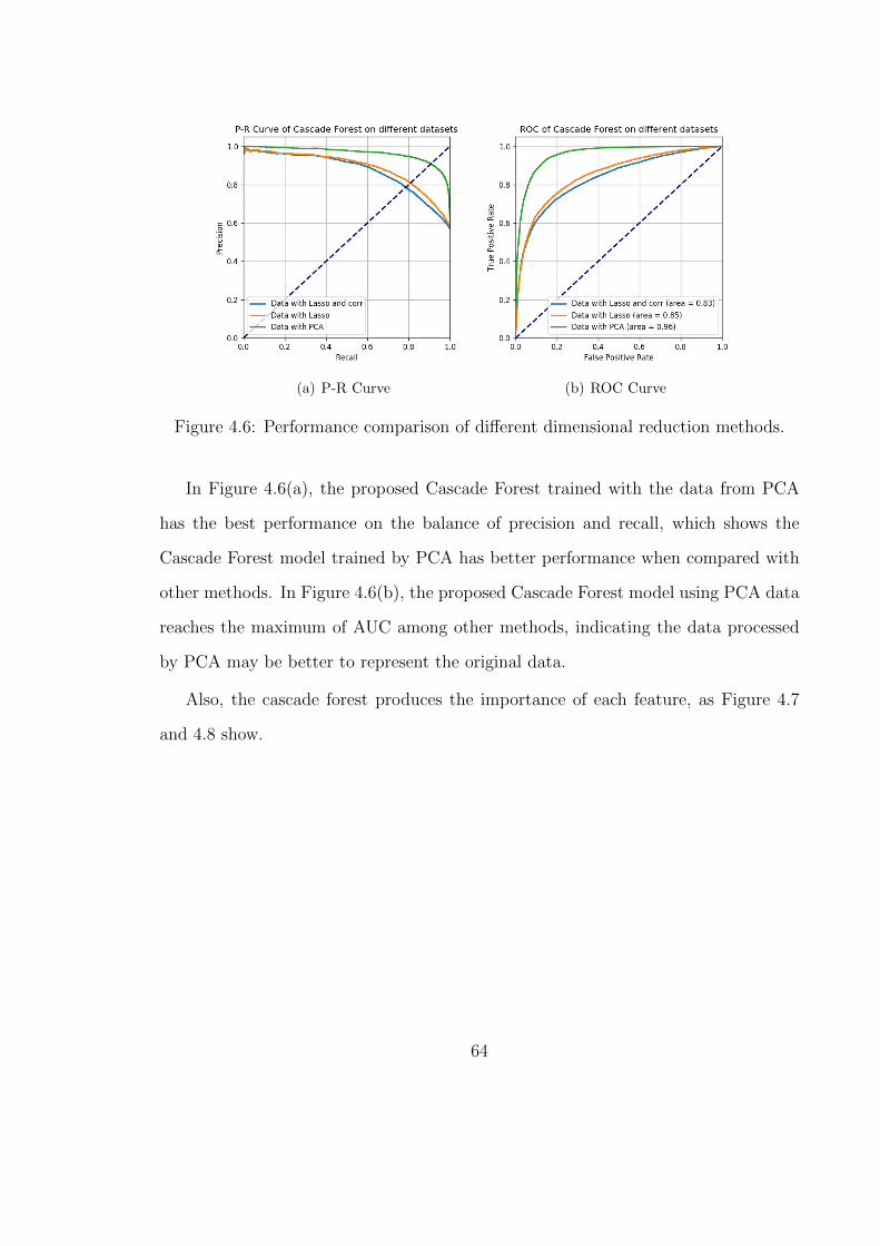
(a) P-R Curve (b) ROC Curve

Figure 4.6: Performance comparison of different dimensional reduction methods.

In Figure 4.6(a), the proposed Cascade Forest trained with the data from PCA

has the best performance on the balance of precision and recall, which shows the

Cascade Forest model trained by PCA has better performance when compared with

other methods. In Figure 4.6(b), the proposed Cascade Forest model using PCA data

reaches the maximum of AUC among other methods, indicating the data processed

by PCA may be better to represent the original data.

Also, the cascade forest produces the importance of each feature, as Figure 4.7

and 4.8 show.

64

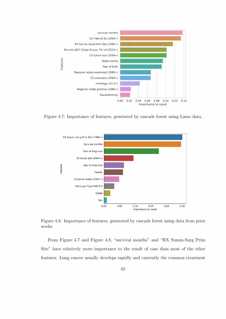
Figure 4.7: Importance of features, generated by cascade forest using Lasso data.

Figure 4.8: Importance of features, generated by cascade forest using data from priorworks.

From Figure 4.7 and Figure 4.8, “survival months” and “RX Summ-Surg Prim

Site” have relatively more importance to the result of case than most of the other

features. Lung cancer usually develops rapidly and currently the common treatment

65

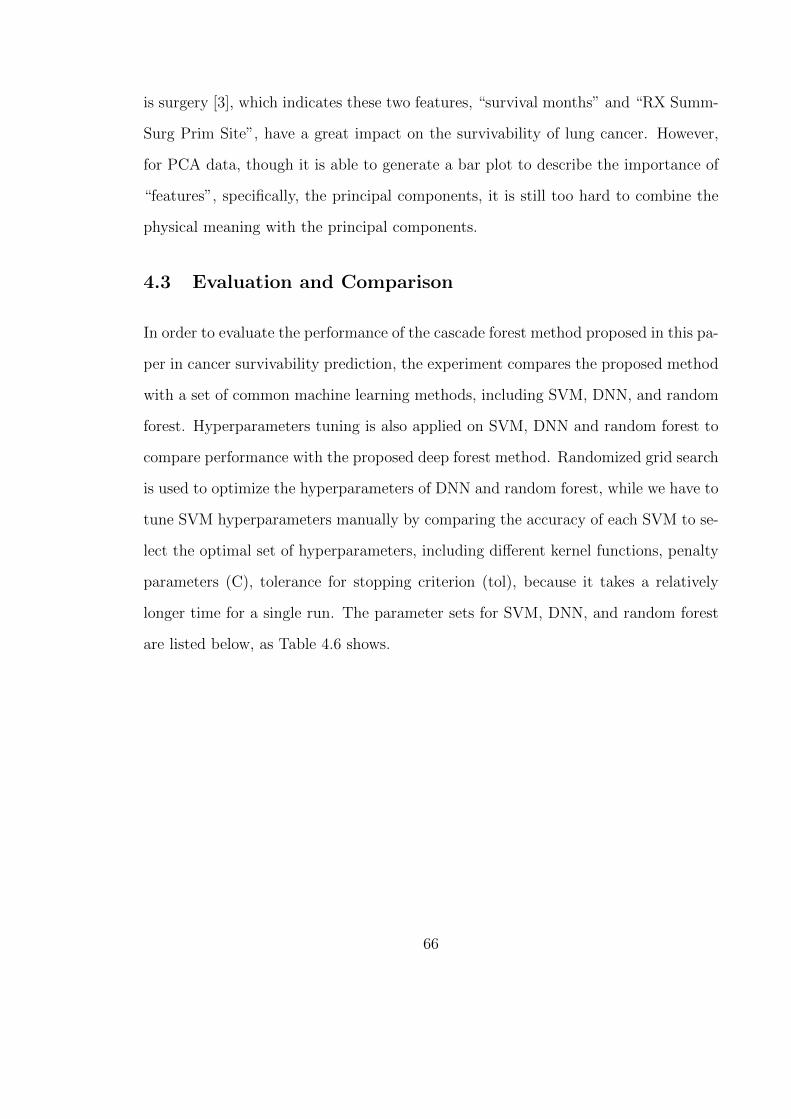
is surgery [3], which indicates these two features, “survival months” and “RX Summ-

Surg Prim Site”, have a great impact on the survivability of lung cancer. However,

for PCA data, though it is able to generate a bar plot to describe the importance of

“features”, specifically, the principal components, it is still too hard to combine the

physical meaning with the principal components.

4.3 Evaluation and Comparison

In order to evaluate the performance of the cascade forest method proposed in this pa-

per in cancer survivability prediction, the experiment compares the proposed method

with a set of common machine learning methods, including SVM, DNN, and random

forest. Hyperparameters tuning is also applied on SVM, DNN and random forest to

compare performance with the proposed deep forest method. Randomized grid search

is used to optimize the hyperparameters of DNN and random forest, while we have to

tune SVM hyperparameters manually by comparing the accuracy of each SVM to se-

lect the optimal set of hyperparameters, including different kernel functions, penalty

parameters (C), tolerance for stopping criterion (tol), because it takes a relatively

longer time for a single run. The parameter sets for SVM, DNN, and random forest

are listed below, as Table 4.6 shows.

66

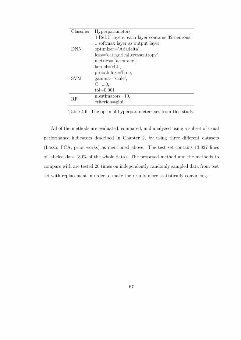
Classifier Hyperparameters

DNN

4 ReLU layers, each layer contains 32 neurons.1 softmax layer as output layeroptimizer=’Adadelta’,loss=’categorical crossentropy’,metrics=[’accuracy’]

SVM

kernel=’rbf’,probability=True,gamma=’scale’,C=1.0,tol=0.001

RFn estimators=10,criterion=gini

Table 4.6: The optimal hyperparameters set from this study.

All of the methods are evaluated, compared, and analyzed using a subset of usual

performance indicators described in Chapter 2, by using three different datasets

(Lasso, PCA, prior works) as mentioned above. The test set contains 13,827 lines

of labeled data (30% of the whole data). The proposed method and the methods to

compare with are tested 20 times on independently randomly sampled data from test

set with replacement in order to make the results more statistically convincing.

67

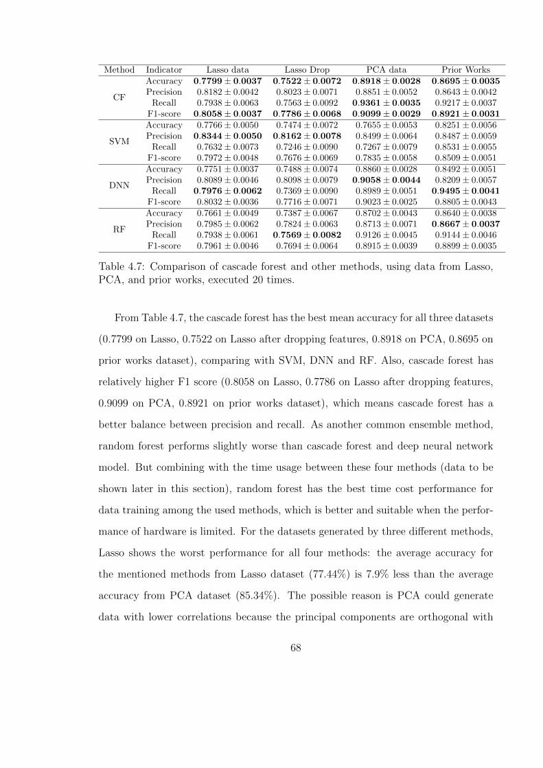
Method Indicator Lasso data Lasso Drop PCA data Prior Works

CF

Accuracy 0.7799± 0.0037 0.7522± 0.0072 0.8918± 0.0028 0.8695± 0.0035Precision 0.8182± 0.0042 0.8023± 0.0071 0.8851± 0.0052 0.8643± 0.0042

Recall 0.7938± 0.0063 0.7563± 0.0092 0.9361± 0.0035 0.9217± 0.0037F1-score 0.8058± 0.0037 0.7786± 0.0068 0.9099± 0.0029 0.8921± 0.0031

SVM

Accuracy 0.7766± 0.0050 0.7474± 0.0072 0.7655± 0.0053 0.8251± 0.0056Precision 0.8344± 0.0050 0.8162± 0.0078 0.8499± 0.0064 0.8487± 0.0059

Recall 0.7632± 0.0073 0.7246± 0.0090 0.7267± 0.0079 0.8531± 0.0055F1-score 0.7972± 0.0048 0.7676± 0.0069 0.7835± 0.0058 0.8509± 0.0051

DNN

Accuracy 0.7751± 0.0037 0.7488± 0.0074 0.8860± 0.0028 0.8492± 0.0051Precision 0.8089± 0.0046 0.8098± 0.0079 0.9058± 0.0044 0.8209± 0.0057

Recall 0.7976± 0.0062 0.7369± 0.0090 0.8989± 0.0051 0.9495± 0.0041F1-score 0.8032± 0.0036 0.7716± 0.0071 0.9023± 0.0025 0.8805± 0.0043

RF

Accuracy 0.7661± 0.0049 0.7387± 0.0067 0.8702± 0.0043 0.8640± 0.0038Precision 0.7985± 0.0062 0.7824± 0.0063 0.8713± 0.0071 0.8667± 0.0037

Recall 0.7938± 0.0061 0.7569± 0.0082 0.9126± 0.0045 0.9144± 0.0046F1-score 0.7961± 0.0046 0.7694± 0.0064 0.8915± 0.0039 0.8899± 0.0035

Table 4.7: Comparison of cascade forest and other methods, using data from Lasso,PCA, and prior works, executed 20 times.

From Table 4.7, the cascade forest has the best mean accuracy for all three datasets

(0.7799 on Lasso, 0.7522 on Lasso after dropping features, 0.8918 on PCA, 0.8695 on

prior works dataset), comparing with SVM, DNN and RF. Also, cascade forest has

relatively higher F1 score (0.8058 on Lasso, 0.7786 on Lasso after dropping features,

0.9099 on PCA, 0.8921 on prior works dataset), which means cascade forest has a

better balance between precision and recall. As another common ensemble method,

random forest performs slightly worse than cascade forest and deep neural network

model. But combining with the time usage between these four methods (data to be

shown later in this section), random forest has the best time cost performance for

data training among the used methods, which is better and suitable when the perfor-

mance of hardware is limited. For the datasets generated by three different methods,

Lasso shows the worst performance for all four methods: the average accuracy for

the mentioned methods from Lasso dataset (77.44%) is 7.9% less than the average

accuracy from PCA dataset (85.34%). The possible reason is PCA could generate

data with lower correlations because the principal components are orthogonal with

68

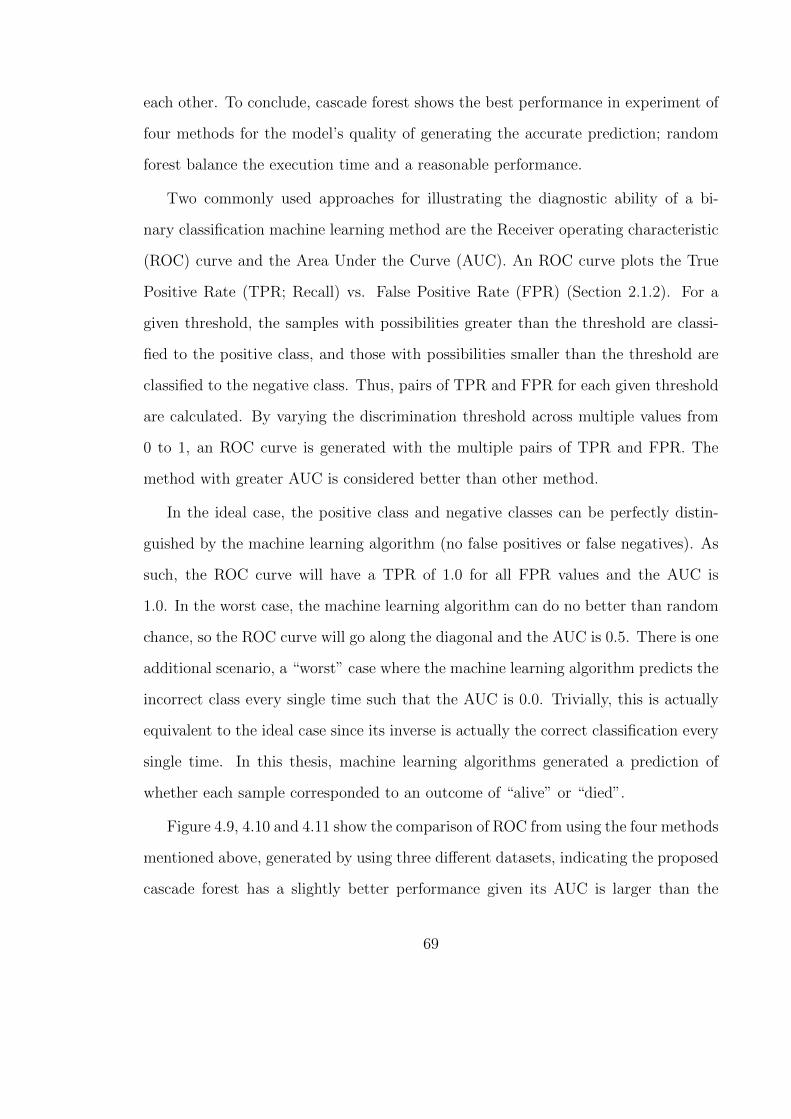
each other. To conclude, cascade forest shows the best performance in experiment of

four methods for the model’s quality of generating the accurate prediction; random

forest balance the execution time and a reasonable performance.

Two commonly used approaches for illustrating the diagnostic ability of a bi-

nary classification machine learning method are the Receiver operating characteristic

(ROC) curve and the Area Under the Curve (AUC). An ROC curve plots the True

Positive Rate (TPR; Recall) vs. False Positive Rate (FPR) (Section 2.1.2). For a

given threshold, the samples with possibilities greater than the threshold are classi-

fied to the positive class, and those with possibilities smaller than the threshold are

classified to the negative class. Thus, pairs of TPR and FPR for each given threshold

are calculated. By varying the discrimination threshold across multiple values from

0 to 1, an ROC curve is generated with the multiple pairs of TPR and FPR. The

method with greater AUC is considered better than other method.

In the ideal case, the positive class and negative classes can be perfectly distin-

guished by the machine learning algorithm (no false positives or false negatives). As

such, the ROC curve will have a TPR of 1.0 for all FPR values and the AUC is

1.0. In the worst case, the machine learning algorithm can do no better than random

chance, so the ROC curve will go along the diagonal and the AUC is 0.5. There is one

additional scenario, a “worst” case where the machine learning algorithm predicts the

incorrect class every single time such that the AUC is 0.0. Trivially, this is actually

equivalent to the ideal case since its inverse is actually the correct classification every

single time. In this thesis, machine learning algorithms generated a prediction of

whether each sample corresponded to an outcome of “alive” or “died”.

Figure 4.9, 4.10 and 4.11 show the comparison of ROC from using the four methods

mentioned above, generated by using three different datasets, indicating the proposed

cascade forest has a slightly better performance given its AUC is larger than the

69

AUC for the other methods for all three datasets. SVM performs with the worst

performance when comparing accross the four different methods.

Figure 4.9: ROC curves on Lasso data.

70

Figure 4.10: ROC curves on data from PCA.

71

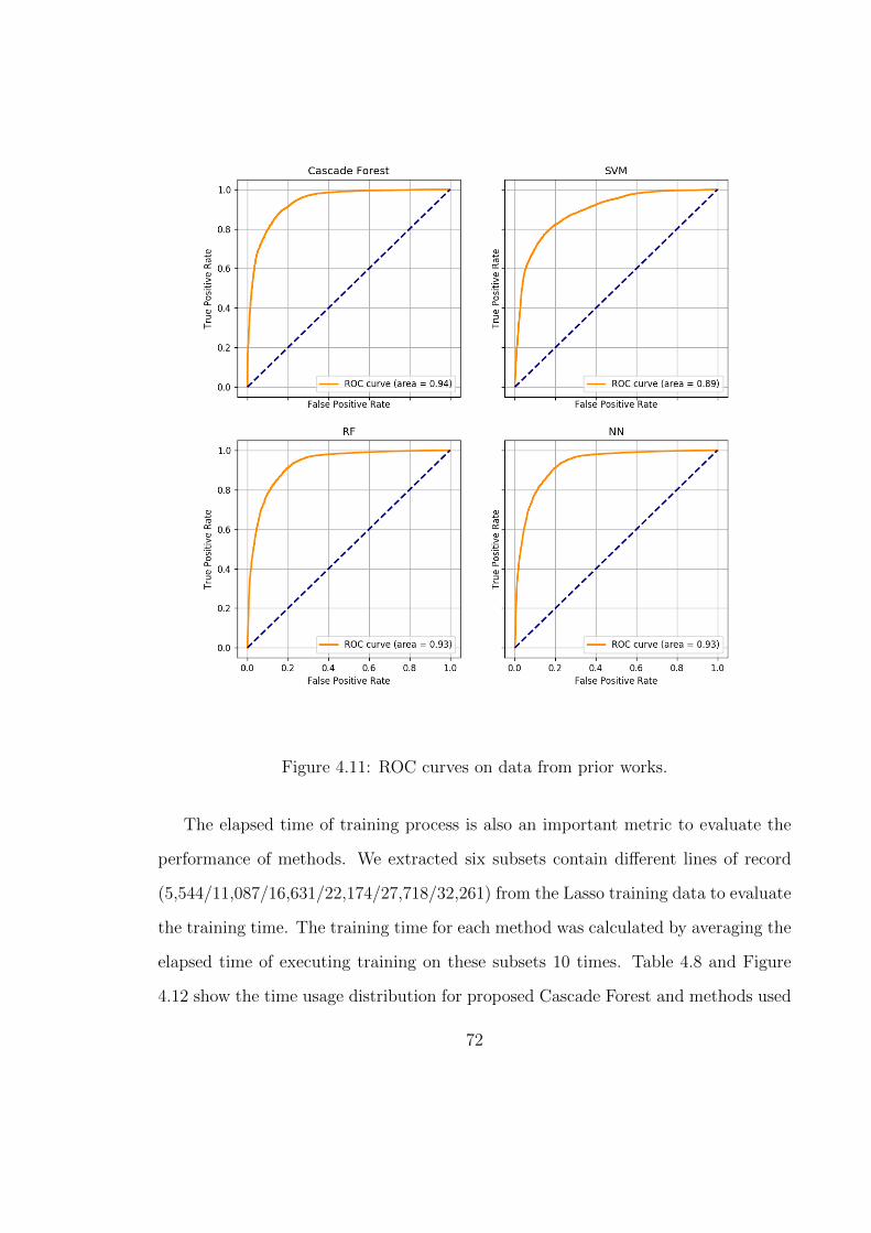
Figure 4.11: ROC curves on data from prior works.

The elapsed time of training process is also an important metric to evaluate the

performance of methods. We extracted six subsets contain different lines of record

(5,544/11,087/16,631/22,174/27,718/32,261) from the Lasso training data to evaluate

the training time. The training time for each method was calculated by averaging the

elapsed time of executing training on these subsets 10 times. Table 4.8 and Figure

4.12 show the time usage distribution for proposed Cascade Forest and methods used

72

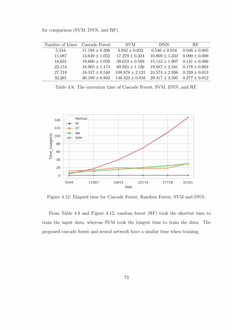
for comparison (SVM, DNN, and RF).

Number of Lines Cascade Forest SVM DNN RF

5,544 11.188± 0.206 3.932± 0.032 6.546± 0.916 0.046± 0.00511,087 13.649± 1.052 17.279± 0.324 10.869± 1.332 0.090± 0.00916,631 19.660± 1.028 39.653± 0.589 15.112± 1.907 0.141± 0.00622,174 16.905± 1.174 69.924± 1.126 19.887± 2.341 0.178± 0.00327,718 18.317± 0.540 108.878± 2.121 24.574± 2.936 0.239± 0.01332,261 30.189± 0.862 146.323± 0.858 29.417± 3.595 0.277± 0.012

Table 4.8: The execution time of Cascade Forest, SVM, DNN, and RF.

Figure 4.12: Elapsed time for Cascade Forest, Random Forest, SVM and DNN.

From Table 4.8 and Figure 4.12, random forest (RF) took the shortest time to

train the input data, whereas SVM took the longest time to train the data. The

proposed cascade forest and neural network have a similar time when training.

73

Chapter 5: Conclusion and future work

This work aimed to apply a new ensemble model, Cascade Forest, on clinical data

to predict lung cancer survivability. With this work, we can conclude an ensemble

deep forest model such as Cascade Forest is suitable for clinical data research whether

the size of input is large or not, because this ensemble decision tree model can change

the growth of layer in an adaptive process, showing a balance of acceptable execution

time and higher accuracy. Moreover, with the development of the multi-core hardware

like GPU in future, parallel distributed algorithm and computation will be more and

more efficient comparing with the conventional methods. Also, the work described in

this thesis brings a new ensemble decision tree method to generate predictions, which

will be helpful for physicians to evaluate the status of their patients, and assist in

making decisions about the proposed therapy of a specific patient.

Possible directions for future work for the applications of deep forest method and

clinical research is abundant. Naturally, the next step is to apply the approach to

genetic data and clinical record together to evaluate the significance of all features, in

order to improve the accuracy of the prediction and indicate which genetic features are

related to a specific type of cancer. We can use multi-grained scanning on the genetic

data to extract more useful relationships in the spatial domain. Additionally, there is

still room to improve the model with respect to time efficiency: the redundant cross-

validation procedure for each node may be optimized to save more time. Moreover,

the hyperparameters for a specific node can be produced by, for example, randomly

increasing the diversity of the model. The hyperparameters can also be inherited and

mutated by genetic algorithm (GA) from the previous layer, as done by F. Friedrichs

et al. [80], using GA to tune the parameters of SVM. That means different random

74

forest nodes in the specific layer could have different hyperparameters, which will

increase the diversity of the layer. This improvement in diversity may have a positive

effect of the accuracy and require a relatively smaller number of executed iterations.

Another possible method is to use weighted averaging (described in Section 3.2) to

integrate the outputs from the individual learners in a layer with those weights and

with the addition of a loss function to be used as part of the training data in the

cascade forest.

75

Bibliography

[1] F. Bray, J. Ferlay, I. Soerjomataram, R. L. Siegel, L. A. Torre, and A. Jemal,

“Global cancer statistics 2018: GLOBOCAN estimates of incidence and mor-

tality worldwide for 36 cancers in 185 countries,” CA: A Cancer Journal for

Clinicians, vol. 68, no. 6, pp. 394–424, 2018, issn: 1542-4863. doi: 10.3322/

caac.21492. [Online]. Available: https://onlinelibrary.wiley.com/doi/

abs/10.3322/caac.21492 (visited on 05/16/2019).

[2] EAPC. (). European association for palliative care, EAPC home, [Online].

Available: https://www.eapcnet.eu/home (visited on 05/17/2019).

[3] SEER Training Modules, Lung cancer, Jan. 5, 2019. [Online]. Available: https:

//training.seer.cancer.gov/lung/.

[4] Surveillance, Epidemiology, and End Results (SEER) Program (www.seer.cancer.gov).

(Nov. 2017). SEER*stat database: Incidence - SEER 18 regs research data +

hurricane katrina impacted louisiana cases, nov 2017 sub (1973-2015 varying) -

linked to county attributes - total u.s., 1969-2016 counties.

[5] (Jun. 13, 2018). The cancer genome atlas, National Cancer Institute, [Online].

Available: https://www.cancer.gov/tcga (visited on 05/29/2019).

[6] A. P. G. Consortium and others, “AACR project GENIE: Powering precision

medicine through an international consortium,” Cancer discovery, vol. 7, no. 8,

pp. 818–831, 2017.

[7] (). Surveillance, epidemiology, and end results program, SEER, [Online]. Avail-

able: https://seer.cancer.gov/index.html (visited on 04/03/2019).

76

[8] D. W. Kim, S. Lee, S. Kwon, W. Nam, I.-H. Cha, and H. J. Kim, “Deep learning-

based survival prediction of oral cancer patients,” Scientific Reports, vol. 9,

no. 1, p. 6994, May 6, 2019, issn: 2045-2322. doi: 10.1038/s41598- 019-

43372-7. [Online]. Available: https://www.nature.com/articles/s41598-

019-43372-7 (visited on 05/16/2019).

[9] D. R. Cox, “Regression models and life-tables,” Journal of the Royal Statistical

Society: Series B (Methodological), vol. 34, no. 2, pp. 187–202, 1972.

[10] K. Kourou, T. P. Exarchos, K. P. Exarchos, M. V. Karamouzis, and D. I.

Fotiadis, “Machine learning applications in cancer prognosis and prediction,”

Computational and Structural Biotechnology Journal, vol. 13, pp. 8 –17, 2015,

issn: 2001-0370. doi: https://doi.org/10.1016/j.csbj.2014.11.005.

[Online]. Available: http://www.sciencedirect.com/science/article/pii/

S2001037014000464.

[11] A. Agrawal, S. Misra, R. Narayanan, L. Polepeddi, and A. Choudhary. (2012).

Lung cancer survival prediction using ensemble data mining on seer data, Scien-

tific Programming, [Online]. Available: https://www.hindawi.com/journals/

sp/2012/920245/abs/ (visited on 04/05/2019).

[12] C. M. Lynch, B. Abdollahi, J. D. Fuqua, A. R. de Carlo, J. A. Bartholomai,

R. N. Balgemann, V. H. van Berkel, and H. B. Frieboes, “Prediction of lung can-

cer patient survival via supervised machine learning classification techniques,”

International Journal of Medical Informatics, vol. 108, pp. 1–8, 2017, issn:

1872-8243. doi: 10.1016/j.ijmedinf.2017.09.013.

[13] C. M. Lynch, V. H. v. Berkel, and H. B. Frieboes, “Application of unsuper-

vised analysis techniques to lung cancer patient data,” PLOS ONE, vol. 12,

no. 9, e0184370, Sep. 14, 2017, issn: 1932-6203. doi: 10 . 1371 / journal .

pone.0184370. [Online]. Available: https://journals.plos.org/plosone/

article?id=10.1371/journal.pone.0184370 (visited on 05/16/2019).

77

[14] Y. Wang, D. Wang, X. Ye, Y. Wang, Y. Yin, and Y. Jin, “A tree ensemble-

based two-stage model for advanced-stage colorectal cancer survival predic-

tion,” Information Sciences, vol. 474, pp. 106–124, Feb. 1, 2019, issn: 0020-

0255. doi: 10.1016/j.ins.2018.09.046. [Online]. Available: http://www.

sciencedirect.com/science/article/pii/S002002551830759X (visited on

05/22/2019).

[15] Z.-H. Zhou and J. Feng, “Deep forest: Towards an alternative to deep neural net-

works,” in Proceedings of the Twenty-Sixth International Joint Conference on

Artificial Intelligence, IJCAI-17, 2017, pp. 3553–3559. doi: 10.24963/ijcai.

2017/497. [Online]. Available: https://doi.org/10.24963/ijcai.2017/497.

[16] Y. LeCun, Y. Bengio, and G. Hinton, “Deep learning,” Nature, vol. 521, p. 436,

May 27, 2015. [Online]. Available: https://doi.org/10.1038/nature14539.

[17] Z.-H. Zhou, Machine Learning. Tsinghua University Press, 2016.

[18] S. Geman, E. Bienenstock, and R. Doursat, “Neural networks and the bias/-

variance dilemma,” Neural Computation, vol. 4, no. 1, pp. 1–58, Jan. 1, 1992,

issn: 0899-7667. doi: 10.1162/neco.1992.4.1.1. [Online]. Available: https:

//doi.org/10.1162/neco.1992.4.1.1 (visited on 05/25/2019).

[19] R. Caruana, S. Lawrence, and C. L. Giles, “Overfitting in neural nets: Back-

propagation, conjugate gradient, and early stopping,” in Advances in neural

information processing systems, 2001, pp. 402–408.

[20] R. Tibshirani, “Regression shrinkage and selection via the lasso,” Journal of the

Royal Statistical Society: Series B (Methodological), vol. 58, no. 1, pp. 267–288,

1996.

[21] J. R. Quinlan, “Induction of decision trees,” Machine Learning, vol. 1, no. 1,

pp. 81–106, Mar. 1, 1986, issn: 1573-0565. doi: 10.1007/BF00116251. [Online].

Available: https://doi.org/10.1007/BF00116251 (visited on 04/21/2019).

78

[22] L. Breiman, Classification and Regression Trees. Routledge, Oct. 19, 2017, isbn:

978-1-351-46049-1. doi: 10.1201/9781315139470. [Online]. Available: https:

//www.taylorfrancis.com/books/9781351460491 (visited on 04/21/2019).

[23] D. Dua and C. Graff, UCI Machine Learning Repository. University of Cal-

ifornia, Irvine, School of Information and Computer Sciences, 2017. [Online].

Available: http://archive.ics.uci.edu/ml.

[24] V. Vapnik and A. Y. Lerner, “Recognition of patterns with help of generalized

portraits,” Avtomat. i Telemekh, vol. 24, no. 6, pp. 774–780, 1963.

[25] J. Listgarten, S. Damaraju, B. Poulin, L. Cook, J. Dufour, A. Driga, J. Mackey,

D. Wishart, R. Greiner, and B. Zanke, “Predictive models for breast cancer

susceptibility from multiple single nucleotide polymorphisms,” Clinical cancer

research, vol. 10, no. 8, pp. 2725–2737, 2004.

[26] J. P. Ehlers and J. W. Harbour, “NBS1 expression as a prognostic marker

in uveal melanoma,” Clinical Cancer Research, vol. 11, no. 5, pp. 1849–1853,

Mar. 1, 2005, issn: 1078-0432, 1557-3265. doi: 10.1158/1078- 0432.CCR-

04-2054. [Online]. Available: http://clincancerres.aacrjournals.org/

content/11/5/1849 (visited on 06/06/2019).

[27] B. E. Boser, I. M. Guyon, and V. N. Vapnik, “A training algorithm for optimal

margin classifiers,” in Proceedings of the Fifth Annual Workshop on Computa-

tional Learning Theory, ser. COLT ’92, event-place: Pittsburgh, Pennsylvania,

USA, New York, NY, USA: ACM, 1992, pp. 144–152, isbn: 978-0-89791-497-0.

doi: 10.1145/130385.130401. [Online]. Available: http://doi.acm.org/10.

1145/130385.130401 (visited on 05/15/2019).

[28] W. S. McCulloch and W. Pitts, “A logical calculus of the ideas immanent in

nervous activity,” The bulletin of mathematical biophysics, vol. 5, no. 4, pp. 115–

133, 1943.

79

[29] F. Rosenblatt, “The perceptron: A probabilistic model for information storage

and organization in the brain.,” Psychological review, vol. 65, no. 6, p. 386, 1958.

[30] Y. LeCun, B. Boser, J. S. Denker, D. Henderson, R. E. Howard, W. Hubbard,

and L. D. Jackel, “Backpropagation applied to handwritten zip code recog-

nition,” Neural Computation, vol. 1, no. 4, pp. 541–551, Dec. 1, 1989, issn:

0899-7667. doi: 10.1162/neco.1989.1.4.541. [Online]. Available: https:

//doi.org/10.1162/neco.1989.1.4.541 (visited on 06/06/2019).

[31] A. Krizhevsky, I. Sutskever, and G. E. Hinton, “ImageNet classification with

deep convolutional neural networks,” in Advances in Neural Information Pro-

cessing Systems 25, F. Pereira, C. J. C. Burges, L. Bottou, and K. Q. Wein-

berger, Eds., Curran Associates, Inc., 2012, pp. 1097–1105. [Online]. Available:

http://papers.nips.cc/paper/4824-imagenet-classification-with-

deep-convolutional-neural-networks.pdf (visited on 06/06/2019).

[32] (Oct. 6, 2015). CUDA toolkit 10.0 download, NVIDIA Developer, [Online].

Available: https://developer.nvidia.com/cuda- downloads (visited on

02/15/2019).

[33] J. Deng, W. Dong, R. Socher, L.-J. Li, K. Li, and L. Fei-Fei, “ImageNet: A

large-scale hierarchical image database,” in CVPR09, 2009.

[34] T. Kohonen, “An introduction to neural computing,” Neural Networks, vol. 1,

no. 1, pp. 3–16, Jan. 1, 1988, issn: 0893-6080. doi: 10.1016/0893-6080(88)

90020- 2. [Online]. Available: http://www.sciencedirect.com/science/

article/pii/0893608088900202 (visited on 04/20/2019).

[35] V. Nair and G. E. Hinton, “Rectified linear units improve restricted boltz-

mann machines,” in Proceedings of the 27th international conference on machine

learning (ICML-10), 2010, pp. 807–814.

[36] A. L. Maas, A. Y. Hannun, and A. Y. Ng, “Rectifier nonlinearities improve

neural network acoustic models,” in Proc. icml, vol. 30, 2013, p. 3.

80

[37] P. Werbos, “Beyond regression: New tools for prediction and analysis in the

behavioral sciences,” Ph. D. dissertation, Harvard University, 1974.

[38] D. E. Rumelhart, G. E. Hinton, R. J. Williams, and others, “Learning repre-

sentations by back-propagating errors,” Cognitive modeling, vol. 5, no. 3, p. 1,

1988.

[39] Y. LeCun, Y. Bengio, and T. B. Laboratories, “Convolutional networks for

images, speech, and time-series,” The handbook of brain theory and neural net-

works, vol. 3361, no. 10, p. 15, 1995.

[40] Y. LeCun, L. Bottou, Y. Bengio, P. Haffner, and others, “Gradient-based learn-

ing applied to document recognition,” Proceedings of the IEEE, vol. 86, no. 11,

pp. 2278–2324, 1998.

[41] D. C. Ciresan, A. Giusti, L. M. Gambardella, and J. Schmidhuber, “Mitosis

detection in breast cancer histology images with deep neural networks,” in In-

ternational Conference on Medical Image Computing and Computer-assisted

Intervention, Springer, 2013, pp. 411–418.

[42] W. Shen, M. Zhou, F. Yang, C. Yang, and J. Tian, “Multi-scale convolutional

neural networks for lung nodule classification,” in International Conference on

Information Processing in Medical Imaging, Springer, 2015, pp. 588–599.

[43] A. Esteva, B. Kuprel, R. A. Novoa, J. Ko, S. M. Swetter, H. M. Blau, and

S. Thrun, “Dermatologist-level classification of skin cancer with deep neural

networks,” Nature, vol. 542, no. 7639, p. 115, 2017.

[44] J. J. Hopfield, “Neural networks and physical systems with emergent collec-

tive computational abilities,” Proceedings of the National Academy of Sciences,

vol. 79, no. 8, pp. 2554–2558, Apr. 1, 1982, issn: 0027-8424, 1091-6490. doi:

10.1073/pnas.79.8.2554. [Online]. Available: https://www.pnas.org/

content/79/8/2554 (visited on 04/21/2019).

81

[45] S. Hochreiter and J. Schmidhuber, “Long short-term memory,” Neural Com-

putation, vol. 9, no. 8, pp. 1735–1780, Nov. 1, 1997, issn: 0899-7667. doi:

10.1162/neco.1997.9.8.1735. [Online]. Available: https://doi.org/

10.1162/neco.1997.9.8.1735 (visited on 04/21/2019).

[46] Z. C. Lipton, J. Berkowitz, and C. Elkan, “A critical review of recurrent neural

networks for sequence learning,” arXiv preprint arXiv:1506.00019, 2015.

[47] N. Razavian, J. Marcus, and D. Sontag, “Multi-task prediction of disease on-

sets from longitudinal laboratory tests,” in Machine Learning for Healthcare

Conference, 2016, pp. 73–100.

[48] M. Guan, S. Cho, R. Petro, W. Zhang, B. Pasche, and U. Topaloglu, “Natu-

ral language processing and recurrent network models for identifying genomic

mutation-associated cancer treatment change from patient progress notes,” JAMIA

Open, vol. 2, no. 1, pp. 139–149, Jan. 3, 2019, issn: 2574-2531. doi: 10 .

1093/jamiaopen/ooy061. [Online]. Available: https://doi.org/10.1093/

jamiaopen/ooy061 (visited on 06/21/2019).

[49] M. Guan, “INCORPORATING EMR AND GENOMIC DATA USING NLP

AND MACHINE LEARNING TO REFINE CANCER TREATMENT,” Dis-

sertation/Thesis, PhD thesis, Wake Forest University, 2018.

[50] S. Sun, C. Yeh, M. Hwang, M. Ostendorf, and L. Xie, “Domain adversarial train-

ing for accented speech recognition,” in 2018 IEEE International Conference on

Acoustics, Speech and Signal Processing (ICASSP), Apr. 2018, pp. 4854–4858.

doi: 10.1109/ICASSP.2018.8462663.

[51] I. Evtimov, K. Eykholt, E. Fernandes, T. Kohno, B. Li, A. Prakash, A. Rah-

mati, and D. Song, “Robust physical-world attacks on deep learning models,”

in Computer Vision and Pattern Recognition, 2018.

[52] B. K. Beaulieu-Jones, Z. S. Wu, C. Williams, R. Lee, S. P. Bhavnani, J. B.

Byrd, and C. S. Greene, “Privacy-preserving generative deep neural networks

82

support clinical data sharing,” bioRxiv, 2018. doi: 10.1101/159756. [Online].

Available: https://www.biorxiv.org/content/early/2018/12/20/159756.

[53] H.-C. Shin, N. A. Tenenholtz, J. K. Rogers, C. G. Schwarz, M. L. Senjem,

J. L. Gunter, K. P. Andriole, and M. Michalski, “Medical image synthesis for

data augmentation and anonymization using generative adversarial networks,”

in Simulation and Synthesis in Medical Imaging, A. Gooya, O. Goksel, I. Oguz,

and N. Burgos, Eds., Springer International Publishing, 2018, pp. 1–11, isbn:

978-3-030-00536-8.

[54] M. Rezaei, K. Harmuth, W. Gierke, T. Kellermeier, M. Fischer, H. Yang, and C.

Meinel, “A conditional adversarial network for semantic segmentation of brain

tumor,” in Brainlesion: Glioma, Multiple Sclerosis, Stroke and Traumatic Brain

Injuries, A. Crimi, S. Bakas, H. Kuijf, B. Menze, and M. Reyes, Eds., Springer

International Publishing, 2018, pp. 241–252, isbn: 978-3-319-75238-9.

[55] (). GeForce GTX 1080 graphics cards | NVIDIA GeForce, [Online]. Available:

https://www.nvidia.com/en-us/geforce/products/10series/geforce-

gtx-1080/ (visited on 04/16/2019).

[56] (). TensorFlow, TensorFlow, [Online]. Available: https://www.tensorflow.

org/ (visited on 02/15/2019).

[57] (). Home - keras documentation, [Online]. Available: https : / / keras . io/

(visited on 02/15/2019).

[58] (). Tensor cores in NVIDIA volta GPU architecture, NVIDIA, [Online]. Avail-

able: https://www.nvidia.com/en-us/data-center/tensorcore/ (visited

on 06/11/2019).

[59] S. Markidis, S. W. D. Chien, E. Laure, I. B. Peng, and J. S. Vetter, “NVIDIA

tensor core programmability, performance precision,” in 2018 IEEE Interna-

tional Parallel and Distributed Processing Symposium Workshops (IPDPSW),

May 2018, pp. 522–531. doi: 10.1109/IPDPSW.2018.00091.

83

[60] P. Haldar, I. D. Pavord, D. E. Shaw, M. A. Berry, M. Thomas, C. E. Brightling,

A. J. Wardlaw, and R. H. Green, “Cluster analysis and clinical asthma pheno-

types,” American journal of respiratory and critical care medicine, vol. 178,

no. 3, pp. 218–224, 2008.

[61] R. W. Tothill, A. V. Tinker, J. George, R. Brown, S. B. Fox, S. Lade, D. S.

Johnson, M. K. Trivett, D. Etemadmoghadam, B. Locandro, and others, “Novel

molecular subtypes of serous and endometrioid ovarian cancer linked to clinical

outcome,” Clinical cancer research, vol. 14, no. 16, pp. 5198–5208, 2008.

[62] S. J. Russell and P. Norvig, Artificial intelligence: a modern approach. Malaysia;

Pearson Education Limited, 2016.

[63] J. X. Chen, “The evolution of computing: AlphaGo,” Computing in Science &

Engineering, vol. 18, no. 4, p. 4, 2016.

[64] I. Goodfellow, Y. Bengio, and A. Courville, Deep learning. MIT press, 2016.

[65] Z. Zhou, Ensemble methods: foundations and algorithms. Chapman and Hal-

l/CRC, 2012.

[66] Y. Freund and R. E. Schapire, “A decision-theoretic generalization of on-line

learning and an application to boosting,” Journal of Computer and System

Sciences, vol. 55, no. 1, pp. 119–139, Aug. 1, 1997, issn: 0022-0000. doi: 10.

1006/jcss.1997.1504. [Online]. Available: http://www.sciencedirect.com/

science/article/pii/S002200009791504X (visited on 05/19/2019).

[67] L. Breiman, “Random forests,” Machine Learning, vol. 45, no. 1, pp. 5–32,

Oct. 1, 2001, issn: 1573-0565. doi: 10.1023/A:1010933404324. [Online]. Avail-

able: https://doi.org/10.1023/A:1010933404324 (visited on 04/17/2019).

[68] Z.-H. Zhou and J. Feng, “Deep forest,” National Science Review, vol. 6, no. 1,

pp. 74–86, Jan. 1, 2019, issn: 2095-5138. doi: 10.1093/nsr/nwy108. [Online].

Available: https://academic.oup.com/nsr/article/6/1/74/5123737

(visited on 04/17/2019).

84

[69] L. V. Utkin, M. S. Kovalev, and A. A. Meldo, “A deep forest classifier with

weights of class probability distribution subsets,” Knowledge-Based Systems,

vol. 173, pp. 15–27, Jun. 1, 2019, issn: 0950-7051. doi: 10.1016/j.knosys.

2019.02.022. [Online]. Available: http://www.sciencedirect.com/science/

article/pii/S0950705119300838 (visited on 05/20/2019).

[70] Y. Guo, S. Liu, Z. Li, and X. Shang, “BCDForest: A boosting cascade deep forest

model towards the classification of cancer subtypes based on gene expression

data,” BMC bioinformatics, vol. 19, pp. 118–13, Suppl 5 2018, issn: 1471-2105.

doi: 10.1186/s12859-018-2095-4.

[71] R. Su, X. Liu, L. Wei, and Q. Zou, “Deep-resp-forest: A deep forest model to

predict anti-cancer drug response,” Methods, Feb. 14, 2019, issn: 1046-2023.

doi: 10.1016/j.ymeth.2019.02.009. [Online]. Available: http://www.

sciencedirect.com/science/article/pii/S1046202318303232 (visited on

06/12/2019).

[72] P. Geurts, D. Ernst, and L. Wehenkel, “Extremely randomized trees,” Machine

Learning, vol. 63, no. 1, pp. 3–42, Apr. 1, 2006, issn: 1573-0565. doi: 10.

1007/s10994-006-6226-1. [Online]. Available: https://doi.org/10.1007/

s10994-006-6226-1 (visited on 04/17/2019).

[73] D. G. Kleinbaum, K Dietz, M Gail, and M. Klein, Logistic regression. Springer,

2002.

[74] (). SEER*stat databases: November 2017 submission, [Online]. Available: https:

//seer.cancer.gov/data-software/documentation/seerstat/nov2017/

(visited on 04/17/2019).

[75] F. Pedregosa, G. Varoquaux, A. Gramfort, V. Michel, B. Thirion, O. Grisel,

M. Blondel, P. Prettenhofer, R. Weiss, V. Dubourg, and others, “Scikit-learn:

Machine learning in python,” Journal of machine learning research, vol. 12,

pp. 2825–2830, Oct 2011.

85

[76] S. J. Wang, S. G. Patel, J. P. Shah, D. P. Goldstein, J. C. Irish, A. L. Carvalho,

L. P. Kowalski, J. L. Lockhart, J. M. Holland, and N. D. Gross, “An oral cav-

ity carcinoma nomogram to predict benefit of adjuvant radiotherapy,” JAMA

Otolaryngology Head and Neck Surgery, vol. 139, no. 6, pp. 554–559, Jun. 1,

2013, issn: 2168-6181. doi: 10.1001/jamaoto.2013.3001. [Online]. Available:

https://jamanetwork.com/journals/jamaotolaryngology/fullarticle/

1686141 (visited on 05/16/2019).

[77] J. Kim and H. Shin, “Breast cancer survivability prediction using labeled, unla-

beled, and pseudo-labeled patient data,” Journal of the American Medical In-

formatics Association, vol. 20, no. 4, pp. 613–618, Jul. 1, 2013, issn: 1067-5027.

doi: 10.1136/amiajnl-2012-001570. [Online]. Available: https://academic.

oup.com/jamia/article/20/4/613/819025 (visited on 01/31/2019).

[78] J. Bergstra and Y. Bengio, “Random search for hyper-parameter optimization,”

Journal of Machine Learning Research, vol. 13, pp. 281–305, Feb 2012.

[79] G. Louppe, “Understanding random forests: From theory to practice,” PhD

thesis, University of Liege, Jul. 28, 2014. arXiv: 1407.7502. [Online]. Available:

http://arxiv.org/abs/1407.7502 (visited on 06/12/2019).

[80] F. Friedrichs and C. Igel, “Evolutionary tuning of multiple SVM parameters,”

Neurocomputing, Trends in Neurocomputing: 12th European Symposium on

Artificial Neural Networks 2004, vol. 64, pp. 107–117, Mar. 1, 2005, issn: 0925-

2312. doi: 10 . 1016 / j . neucom . 2004 . 11 . 022. [Online]. Available: http :

/ / www . sciencedirect . com / science / article / pii / S0925231204005223

(visited on 04/17/2019).

86

Appendix A: Description of Variables in SEER Dataset

The description of variables in SEER Dataset is from the official SEER website

[4].

87

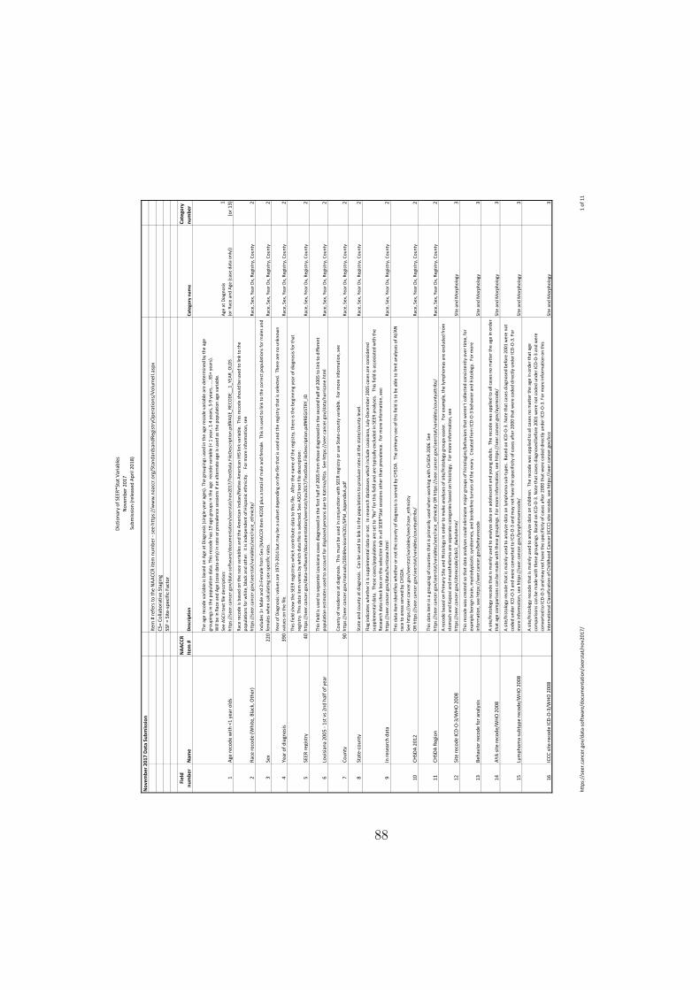
Dict

iona

ry o

f SEE

R*St

at V

aria

bles

N

ovem

ber 2

017

Sub

mis

sion

(rel

ease

d Ap

ril 2

018)

http

s://

seer

.can

cer.g

ov/d

ata-

soft

war

e/do

cum

enta

tion/

seer

stat

/nov

2017

/1

of 1

1

Nov

embe

r 201

7 D

ata

Subm

issi

onIte

m #

refe

rs to

the

NAA

CCR

item

num

ber -

see

http

s://

ww

w.n

aacc

r.org

/Sta

ndar

dsan

dReg

istr

yOpe

ratio

ns/V

olum

eII.a

spx

CS=

Colla

bora

tive

Stag

ing

SSF

= Si

te-s

peci

fic F

acto

r

Fiel

d nu

mbe

rN

ame

NAA

CCR

Item

#D

escr

iptio

nCa

tego

ry n

ame

Cate

gory

nu

mbe

r

1Ag

e re

code

with

<1

year

old

s

The

age

reco

de v

aria

ble

is ba

sed

on A

ge a

t Dia

gnos

is (s

ingl

e-ye

ar a

ges)

. The

gro

upin

gs u

sed

in th

e ag

e re

code

var

iabl

e ar

e de

term

ined

by

the

age

grou

ping

s in

the

popu

latio

n da

ta. T

his r

ecod

e ha

s 19

age

grou

ps in

the

age

reco

de v

aria

ble

(< 1

yea

r, 1-

4 ye

ars,

5-9

yea

rs, .

.., 8

5+ y

ears

).

Will

be

in R

ace

and

Age

(cas

e da

ta o

nly)

in ra

te o

r pre

vale

nce

sess

ions

if a

n al

tern

ate

age

is us

ed a

s the

pop

ulat

ion

age

varia

ble.

See

ASCI

I tex

t file

des

crip

tion:

http

s://

seer

.can

cer.g

ov/d

ata-

soft

war

e/do

cum

enta

tion/

seer

stat

/nov

2017

/Tex

tDat

a.Fi

leDe

scrip

tion.

pdf#

AGE_

RECO

DE__

1_YE

AR_O

LDS

Age

at D

iagn

osis

(or R

ace

and

Age

(cas

e da

ta o

nly)

)1

(or 1

3)

2Ra

ce re

code

(Whi

te, B

lack

, Oth

er)

Race

reco

de is

bas

ed o

n th

e ra

ce v

aria

bles

and

the

Amer

ican

Indi

an/N

ativ

e Am

eric

an IH

S lin

k va

riabl

e. T

his r

ecod

e sh

ould

be

used

to li

nk to

the

popu

latio

ns fo

r whi

te, b

lack

and

oth

er.

It is

inde

pend

ent o

f Hisp

anic

eth

nici

ty.

For

mor

e in

form

atio

n, se

e ht

tps:

//se

er.c

ance

r.gov

/see

rsta

t/va

riabl

es/s

eer/

race

_eth

nici

ty/

Race

, Sex

, Yea

r Dx,

Reg

istry

, Cou

nty

2

3Se

x22

0In

clud

es 1

= M

ale

and

2=Fe

mal

e fr

om S

ex [N

AACC

R Ite

m #

220]

plu

s a to

tal o

f mal

e an

d fe

mal

e. T

his i

s use

d to

link

to th

e co

rrec

t pop

ulat

ions

for m

ales

and

fe

mal

es w

hen

calc

ulat

ing

sex-

spec

ific

rate

s.Ra

ce, S

ex, Y

ear D

x, R

egist

ry, C

ount

y2

4Ye

ar o

f dia

gnos

is39

0Ye

ar o

f Dia

gnos

is: v

alue

s are

197

3-20

14 b

ut m

ay b

e a

subs

et d

epen

ding

on

the

file

that

is u

sed

and

the

regi

stry

that

is se

lect

ed.

Ther

e ar

e no

unk

now

n va

lues

on

the

file.

Race

, Sex

, Yea

r Dx,

Reg

istry

, Cou

nty

2

5SE

ER re

gist

ry40

This

field

show

the

SEER

regi

strie

s whi

ch c

ontr

ibut

e da

ta to

this

file.

Aft

er th

e na

me

of th

e re

gist

ry, t

here

is th

e be

ginn

ing

year

of d

iagn

osis

for t

hat

regi

stry

. Thi

s dat

a ite

m v

arie

s by

whi

ch d

ata

file

is se

lect

ed. S

ee A

SCII

text

file

des

crip

tion:

ht

tps:

//se

er.c

ance

r.gov

/dat

a-so

ftw

are/

docu

men

tatio

n/se

erst

at/n

ov20

17/T

extD

ata.

File

Desc

riptio

n.pd

f#RE

GIS

TRY_

IDRa

ce, S

ex, Y

ear D

x, R

egist

ry, C

ount

y2

6Lo

uisi

ana

2005

- 1s

t vs 2

nd h

alf o

f yea

rTh

is fie

ld is

use

d to

sepa

rate

Lou

isian

a ca

ses d

iagn

osed

in th

e fir

st h

alf o

f 200

5 fr

om th

ose

diag

nose

d in

the

seco

nd h

alf o

f 200

5 to

link

to d

iffer

ent

popu

latio

n es

timat

es u

sed

to a

ccou

nt fo

r disp

lace

d pe

rson

s due

to K

atrin

a/Ri

ta.

See

http

s://

seer

.can

cer.g

ov/d

ata/

hurr

ican

e.ht

ml

Race

, Sex

, Yea

r Dx,

Reg

istry

, Cou

nty

2

7Co

unty

90Co

unty

of r

esid

ence

at d

iagn

osis.

Thi

s mus

t be

used

in c

onju

nctio

n w

ith S

EER

regi

stry

or u

se S

tate

-cou

nty

varia

ble.

For

mor

e in

form

atio

n, se

e ht

tps:

//se

er.c

ance

r.gov

/man

uals/

2004

Revi

sion%

201/

SPM

_App

endi

xA.p

dfRa

ce, S

ex, Y

ear D

x, R

egist

ry, C

ount

y2

8St

ate-

coun

tySt

ate

and

coun

ty a

t dia

gnos

is. C

an b

e us

ed to

link

to th

e po

pula

tions

to p

rodu

ce ra

tes a

t the

stat

e/co

unty

leve

l.Ra

ce, S

ex, Y

ear D

x, R

egist

ry, C

ount

y2

9In

rese

arch

dat

a

Flag

indi

cate

s whe

ther

it is

supp

lem

enta

l dat

a or

not

. In

rese

arch

dat

abas

es w

hich

incl

ude

Loui

siana

, Jul

y-De

cem

ber 2

005

case

s are

con

sider

ed

supp

lem

enta

l dat

a. T

hese

cas

es/p

opul

atio

ns a

re se

t to

"No"

for t

his f

ield

and

are

typi

cally

exc

lude

d in

SEE

R an

alys

es.

Thi

s fie

ld is

ass

ocia

ted

with

the

Rese

arch

dat

a ch

eck

box

on th

e se

lect

ion

tab

in a

ll SE

ER*S

tat s

essio

ns o

ther

than

pre

vale

nce.

For

mor

e in

form

atio

n, se

e:

http

s://

seer

.can

cer.g

ov/d

ata/

hurr

ican

e.ht

ml

Race

, Sex

, Yea

r Dx,

Reg

istry

, Cou

nty

2

10CH

SDA

2012

This

data

item

iden

tifie

s whe

ther

or n

ot th

e co

unty

of d

iagn

osis

is se

rved

by

CHSD

A. T

he p

rimar

y us

e of

this

field

is to

be

able

to li

mit

anal

yses

of A

I/AN

ra

ce to

are

as se

rved

by

CHSD

A.

See

http

s://

seer

.can

cer.g

ov/s

eers

tat/

varia

bles

/see

r/ra

ce_e

thni

city

O

R ht

tps:

//se

er.c

ance

r.gov

/see

rsta

t/va

riabl

es/c

ount

yatt

ribs/

Race

, Sex

, Yea

r Dx,

Reg

istry

, Cou

nty

2

11CH

SDA

Regi

onTh

is da

ta it

em is

a g

roup

ing

of c

ount

ies t

hat i

s prim

arily

use

d w

hen

wor

king

with

CHS

DA 2

006.

See

ht

tps:

//se

er.c

ance

r.gov

/see

rsta

t/va

riabl

es/s

eer/

race

_eth

nici

ty O

R ht

tps:

//se

er.c

ance

r.gov

/see

rsta

t/va

riabl

es/c

ount

yatt

ribs/

Race

, Sex

, Yea

r Dx,

Reg

istry

, Cou

nty

2

12Si

te re

code

ICD-

O-3

/WHO

200

8

A re

code

bas

ed o

n Pr

imar

y Si

te a

nd H

istol

ogy

in o

rder

to m

ake

anal

yses

of s

ite/h

istol

ogy

grou

ps e

asie

r. F

or e

xam

ple,

the

lym

phom

as a

re e

xclu

ded

from

st

omac

h an

d Ka

posi

and

mes

othe

liom

a ar

e se

para

te c

ateg

orie

s bas

ed o

n hi

stol

ogy.

For

mor

e in

form

atio

n, se

e ht

tps:

//se

er.c

ance

r.gov

/site

reco

de/ic

do3_

dwho

hem

e/Si

te a

nd M

orph

olog

y3

13Be

havi

or re

code

for a

naly

sis

This

reco

de w

as c

reat

ed so

that

dat

a an

alys

es c

ould

elim

inat

e m

ajor

gro

ups o

f hist

olog

ies/

beha

vior

s tha

t wer

en't

colle

cted

con

siste

ntly

ove

r tim

e, fo

r ex

ampl

e be

nign

bra

in, m

yelo

dypl

astic

synd

rom

es, a

nd b

orde

rline

tum

ors o

f the

ova

ry.

Crea

ted

from

ICD-

O-3

beh

avio

r and

hist

olog

y. F

or m

ore

info

rmat

ion,

see

http

s://

seer

.can

cer.g

ov/b

ehav

reco

deSi

te a

nd M

orph

olog

y3

14AY

A si

te re

code

/WHO

200

8A

site/

hist

olog

y re

code

that

is m

ainl

y us

ed to

ana

lyze

dat

a on

ado

lesc

ent a

nd y

oung

adu

lts.

The

reco

de w

as a

pplie

d to

all

case

s no

mat

ter t

he a

ge in

ord

er

that

age

com

paris

ons c

an b

e m

ade

with

thes

e gr

oupi

ngs.

For

mor

e in

form

atio

n, se

e ht

tps:

//se

er.c

ance

r.gov

/aya

reco

de/

Site

and

Mor

phol

ogy

3

15Ly

mph

oma

subt

ype

reco

de/W

HO 2

008

A sit

e/hi

stol

ogy

reco

de th

at is

mai

nly

used

to a

naly

ze d

ata

on ly

mph

oma

sub-

type

s. B

ased

on

ICD-

O-3

. Not

e th

at c

ases

dia

gnos

ed b

efor

e 20

01 w

ere

not

code

d un

der I

CD-O

-3 a

nd w

ere

conv

erte

d to

ICD-

O-3

and

may

not

hav

e th

e sp

ecifi

city

of c

ases

aft

er 2

000

that

wer

e co

ded

dire

ctly

und

er IC

D-O

-3. F

or

mor

e in

form

atio

n, se

e ht

tps:

//se

er.c

ance

r.gov

/lym

phom

arec

ode/

Site

and

Mor

phol

ogy

3

16IC

CC si

te re

code

ICD-

O-3

/WHO

200

8

A sit

e/hi

stol

ogy

reco

de th

at is

mai

nly

used

to a

naly

ze d

ata

on c

hild

ren.

The

reco

de w

as a

pplie

d to

all

case

s no

mat

ter t

he a

ge in

ord

er th

at a

ge

com

paris

ons c

an b

e m

ade

with

thes

e gr

oupi

ngs.

Bas

ed o

n IC

D-O

-3. N

ote

that

cas

es d

iagn

osed

bef

ore

2001

wer

e no

t cod

ed u

nder

ICD-

O-3

and

wer

e co

nver

ted

to IC

D-O

-3 a

nd m

ay n

ot h

ave

the

spec

ifici

ty o

f cas

es a

fter

200

0 th

at w

ere

code

d di

rect

ly u

nder

ICD-

O-3

. For

mor

e in

form

atio

n on

this

Inte

rnat

iona

l Cla

ssifi

catio

n of

Chi

ldho

od C

ance

r (IC

CC) s

ite re

code

, see

htt

ps:/

/see

r.can

cer.g

ov/ic

ccSi

te a

nd M

orph

olog

y3

88

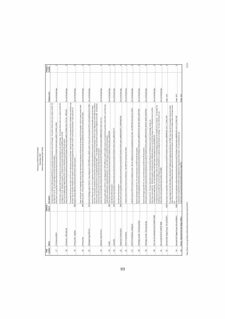
Dict

iona

ry o

f SEE

R*St

at V

aria

bles

N

ovem

ber 2

017

Sub

mis

sion

(rel

ease

d Ap

ril 2

018)

http

s://

seer

.can

cer.g

ov/d

ata-

soft

war

e/do

cum

enta

tion/

seer

stat

/nov

2017

/2

of 1

1

Fiel

d nu

mbe

rN

ame

NAA

CCR

Item

#D

escr

iptio

nCa

tego

ry n

ame

Cate

gory

nu

mbe

r

17CS

Sch

ema

v020

4+

CS in

form

atio

n is

colle

cted

und

er th

e sp

ecifi

catio

ns o

f a p

artic

ular

sche

ma

base

d on

site

and

hist

olog

y. T

his r

ecod

e sh

ould

use

d in

any

ana

lysis

of A

JCC

7th

ed st

age

and

T, N

, M.

For m

ore

info

rmat

ion

see

ASCI

I tex

t file

des

crip

tion:

ht

tps:

//se

er.c

ance

r.gov

/dat

a-so

ftw

are/

docu

men

tatio

n/se

erst

at/n

ov20

17/T

extD

ata.

File

Desc

riptio

n.pd

f#CS

_SCH

EMA_

v020

4_Si

te a

nd M

orph

olog

y3

18CS

Sch

ema

- AJC

C 6t

h ed

CS in

form

atio

n is

colle

cted

und

er th

e sp

ecifi

catio

ns o

f a p

artic

ular

sche

ma

base

d on

site

and

hist

olog

y. T

his r

ecod

e sh

ould

use

d in

any

ana

lysis

of A

JCC

6th

ed st

age

and

T, N

, M.

Base

d on

CS

vers

ion

1, it

shou

ld n

ot b

e us

ed fo

r SSF

s col

lect

ed o

r mod

ified

und

er C

S v0

2.

http

s://

canc

erst

agin

g.or

g/cs

tage

/sch

ema.

htm

l. Fo

r mor

e in

form

atio

n se

e AS

CII t

ext f

ile d

escr

iptio

n:

http

s://

seer

.can

cer.g

ov/d

ata-

soft

war

e/do

cum

enta

tion/

seer

stat

/nov

2017

/Tex

tDat

a.Fi

leDe

scrip

tion.

pdf#

CS_S

CHEM

A_AJ

CC_6

TH_E

D__P

REVI

OU

SSi

te a

nd M

orph

olog

y3

19Pr

imar

y Si

te -

labe

led

400

This

prov

ides

the

prim

ary

site

code

in IC

D-O

-3 a

nd a

des

crip

tive

prim

ary

site

labe

l. N

ote

that

the

labe

l is t

he p

refe

rred

ICD-

O-3

bol

ded

nam

e an

d th

ere

may

be

oth

er si

tes o

r sub

-site

s inc

lude

d in

the

code

but

not

refle

cted

in th

e pr

efer

red

term

. Ref

er to

ICD-

O-3

for f

urth

er in

form

atio

n. C

ases

with

yea

rs o

f di

agno

sis b

efor

e 19

92 w

ere

conv

erte

d to

ICD-

O-3

from

ear

lier v

ersio

ns.

Site

and

Mor

phol

ogy

3

20Pr

imar

y Si

te40

0Co

des a

re fo

und

in th

e To

pogr

aphy

sect

ion

of th

e In

tern

atio

nal C

lass

ifica

tion

of D

iseas

es fo

r Onc

olog

y (IC

D-O

) 3rd

edi

tion.

ICD

-O-2

cod

es u

sed

for 1

992-

2000

are

sim

ilar.

Prim

ary

site

code

s for

197

3-19

91 w

ere

conv

erte

d to

ICD-

O-3

and

may

lack

the

spec

ifici

ty o

f the

ICD-

O-3

prim

ary

site

code

s.

Site

and

Mor

phol

ogy

3

21Hi

stol

ogic

Typ

e IC

D-O

-352

2Ba

sed

on h

istol

ogy

code

s in

ICD-

O-3

. Ca

ses d

iagn

osed

in 1

973-

2000

wer

e co

ded

in e

arlie

r ver

sions

and

con

vert

ed to

ICD-

O-3

and

cod

ed d

irect

ly fo

r 200

1+.

Site

and

Mor

phol

ogy

3

22Be

havi

or c

ode

ICD-

O-3

Base

d on

beh

avio

r cod

es in

ICD-

O-3

. Beh

avio

r cod

e ha

s had

the

sam

e de

finiti

ons i

n pr

evio

us v

ersio

ns b

ut m

ay b

e as

soci

ated

diff

eren

tly w

ith h

istol

ogie

s ov

er ti

me.

For

exa

mpl

e, b

orde

rline

of t

he o

vary

wer

e co

nsid

ered

mal

igna

nt in

ICD-

O-2

but

ben

ign

in IC

D-O

-3. c

ases

dia

gnos

ed in

197

3-20

00 w

ere

code

d in

ea

rlier

ver

sions

and

con

vert

ed to

ICD-

O-3

and

cod

ed d

irect

ly fo

r 200

1+.

In si

tu b

ladd

er c

ases

hav

e be

en c

onve

rted

to m

alig

nant

in th

is fie

ld.

See

Beha

vior

re

code

for c

onsis

tenc

y ov

er ti

me.

For

mor

e in

form

atio

n se

e AS

CII t

ext f

ile d

escr

iptio

n:

http

s://

seer

.can

cer.g

ov/d

ata-

soft

war

e/do

cum

enta

tion/

seer

stat

/nov

2017

/Tex

tDat

a.Fi

leDe

scrip

tion.

pdf#

BEHA

VIO

R_CO

DE_I

CD_O

_3Si

te a

nd M

orph

olog

y3

23G

rade

440

Base

d on

gra

de c

odes

in IC

D-O

-3.

Case

s dia

gnos

ed in

197

3-20

00 w

ere

code

d in

ear

lier v

ersio

ns a

nd m

ay la

ck th

e sp

ecifi

city

of t

he 2

001+

cas

es th

at w

ere

code

d di

rect

ly, e

spec

ially

for l

ymph

omas

/leuk

emia

s. F

or m

ore

info

rmat

ion

see

ASCI

I tex

t file

des

crip

tion:

ht

tps:

//se

er.c

ance

r.gov

/dat

a-so

ftw

are/

docu

men

tatio

n/se

erst

at/n

ov20

17/T

extD

ata.

File

Desc

riptio

n.pd

f#G

RADE

Site

and

Mor

phol

ogy

3

24La

tera

lity

410

See

ASCI

I tex

t file

des

crip

tion:

ht

tps:

//se

er.c

ance

r.gov

/dat

a-so

ftw

are/

docu

men

tatio

n/se

erst

at/n

ov20

17/T

extD

ata.

File

Desc

riptio

n.pd

f#LA

TERA

LITY

Site

and

Mor

phol

ogy

3

25Di

agno

stic

Con

firm

atio

n49

0Se

e AS

CII t

ext f

ile d

escr

iptio

n:

http

s://

seer

.can

cer.g

ov/d

ata-

soft

war

e/do

cum

enta

tion/

seer

stat

/nov

2017

/Tex

tDat

a.Fi

leDe

scrip

tion.

pdf#

DIAG

NO

STIC

_CO

NFI

RMAT

ION

Site

and

Mor

phol

ogy

3

26IC

D-O

-3 H

ist/

beha

vLa

bele

d ve

rsio

n of

ICD-

O-3

val

ues f

or a

ll be

havi

ors.

See

SEE

R*St

at d

ictio

nary

for l

abel

s.Si

te a

nd M

orph

olog

y3

27IC

D-O

-3 H

ist/

beha

v, m

alig

nant

Labe

led

vers

ion

of IC

D-O

-3 v

alue

s for

mal

igna

nt tu

mor

s. A

ll no

n-m

alig

nant

tum

ors a

re g

roup

ed in

to o

ne v

alue

. Se

e SE

ER*S

tat d

ictio

nary

for l

abel

s.Si

te a

nd M

orph

olog

y3

28Hi

stol

ogy

reco

de -

broa

d gr

oupi

ngs

Base

d on

Hist

olog

ic ty

pe IC

D-O

-3.

For m

ore

info

rmat

ion

see

ASCI

I tex

t file

des

crip

tion:

http

s://

seer

.can

cer.g

ov/d

ata-

soft

war

e/do

cum

enta

tion/

seer

stat

/nov

2017

/Tex

tDat

a.Fi

leDe

scrip

tion.

pdf#

HIST

OLO

GY_

RECO

DE_B

RAIN

_GRO

UPI

NG

Site

and

Mor

phol

ogy

3

29Hi

stol

ogy

reco

de -

brai

n gr

oupi

ngs

Base

d on

Hist

olog

ic ty

pe IC

D-O

-3.

For m

ore

info

rmat

ion

see

ASCI

I tex

t file

des

crip

tion:

ht

tps:

//se

er.c

ance

r.gov

/dat

a-so

ftw

are/

docu

men

tatio

n/se

erst

at/n

ov20

17/T

extD

ata.

File

Desc

riptio

n.pd

f#HI

STO

LOG

Y_RE

CODE

_BRA

IN_G

ROU

PIN

GSi

te a

nd M

orph

olog

y3

30IC

CC si

te re

c ex

tend

ed IC

D-O

-3/W

HO 2

008

Base

d on

ICD-

O-3

. Fo

r mor

e in

form

atio

n on

this

Inte

rnat

iona

l Cla

ssifi

catio

n of

Chi

ldho

od C

ance

r (IC

CC) s

ite/h

istol

ogy

reco

de, s

ee

http

s://

seer

.can

cer.g

ov/ic

cc.

Whi

le th

e re

code

is n

orm

ally

use

d fo

r chi

ldho

od c

ance

rs, i

t is o

n th

e fil

e fo

r all

ages

so th

at c

hild

hood

can

cers

cou

ld b

e co

mpa

red

acro

ss a

ge g

roup

s. F

or m

ore

info

rmat

ion,

see

http

s://

seer

.can

cer.g

ov/ic

cc/ic

cc-w

ho20

08.h

tml

Site

and

Mor

phol

ogy

3

31Si

te re

code

B IC

D-O

-3/W

HO 2

008

A re

code

bas

ed o

n Pr

imar

y Si

te a

nd H

istol

ogy

in o

rder

to m

ake

anal

yses

of s

ite/h

istol

ogy

grou

ps e

asie

r for

mul

tiple

prim

ary

anal

yses

. F

or e

xam

ple,

the

lym

phom

as a

re e

xclu

ded

from

stom

ach

and

Kapo

si an

d m

esot

helio

ma

are

sepa

rate

cat

egor

ies b

ased

on

hist

olog

y. F

or m

ore

info

rmat

ion,

see

http

s://

seer

.can

cer.g

ov/s

itere

code

_b/ic

do3_

who

2008

/Si

te a

nd M

orph

olog

y3

32De

rived

AJC

C St

age

Gro

up, 7

th e

d (2

010+

)34

30ht

tps:

//se

er.c

ance

r.gov

/dat

a-so

ftw

are/

docu

men

tatio

n/se

erst

at/n

ov20

17/T

extD

ata.

File

Desc

riptio

n.pd

f#DE

RIVE

D_AJ

CC_7

_STA

GE_

GRP

Stag

e - A

JCC

4

33De

rived

AJC

C St

age

Gro

up, 6

th e

d (2

004+

)30

00

The

stag

e ca

tego

ry fo

r AJC

C 6t

h ed

ition

is d

eriv

ed fr

om C

olla

bora

tive

Stag

ing

data

ele

men

ts fo

r 200

4+ c

ases

. See

the

CS si

te-s

peci

fic sc

hem

a fo

r det

ails

(htt

ps:/

/see

r.can

cer.g

ov/s

eers

tat/

varia

bles

/see

r/aj

cc-s

tage

) and

the

ASCI

I tex

t file

des

crip

tion

for a

llow

able

val

ues f

or d

ispla

y co

des a

nd st

orag

e va

lues

. Se

eht

tps:

//se

er.c

ance

r.gov

/dat

a-so

ftw

are/

docu

men

tatio

n/se

erst

at/n

ov20

17/T

extD

ata.

File

Desc

riptio

n.pd

f#DE

RIVE

D_AJ

CC_6

_STA

GE_

GRP

Stag

e - A

JCC

4

34Br

east

- Ad

just

ed A

JCC

6th

Stag

e (1

988+

)Cr

eate

d fr

om m

erge

d EO

D 3r

d Ed

ition

and

Col

labo

rativ

e St

age

dise

ase

info

rmat

ion.

For

mor

e in

form

atio

n se

e:

http

s://

seer

.can

cer.g

ov/s

eers

tat/

varia

bles

/see

r/aj

cc-s

tage

/6th

/.St

age

- AJC

C

89

Dict

iona

ry o

f SEE

R*St

at V

aria

bles

N

ovem

ber 2

017

Sub

mis

sion

(rel

ease

d Ap

ril 2

018)

http

s://

seer

.can

cer.g

ov/d

ata-

soft

war

e/do

cum

enta

tion/

seer

stat

/nov

2017

/3

of 1

1

Fiel

d nu

mbe

rN

ame

NAA

CCR

Item

#D

escr

iptio

nCa

tego

ry n

ame

Cate

gory

nu

mbe

r

35De

rived

AJC

C - F

lag

(200

4+)

3030

This

flag

curr

ently

refle

cts o

nly

whe

n AJ

CC st

age

is de

rived

bas

ed o

n CS

. If

AJCC

stag

e is

deriv

ed b

ased

on

case

s bef

ore

2004

, it w

ill c

urre

ntly

be

foun

d in

a

sepa

rate

fiel

d an

d no

t ove

rlaye

d in

the

Deriv

ed A

JCC

field

s.

See

ASCI

I tex

t file

des

crip

tion:

ht

tps:

//se

er.c

ance

r.gov

/dat

a-so

ftw

are/

docu

men

tatio

n/se

erst

at/n

ov20

17/T

extD

ata.

File

Desc

riptio

n.pd

f#DE

RIVE

D_AJ

CC_F

LAG

Stag

e - A

JCC

4

36AJ

CC st

age

3rd

editi

on (1

988-

2003

)De

rived

by

algo

rithm

from

ext

ent o

f dise

ase

(EO

D).

Not

ava

ilabl

e fo

r all

year

s or f

or a

ll sit

es. S

ee A

SCII

text

file

des

crip

tion:

ht

tps:

//se

er.c

ance

r.gov

/dat

a-so

ftw

are/

docu

men

tatio

n/se

erst

at/n

ov20

17/T

extD

ata.

File

Desc

riptio

n.pd

f#AJ

CC_S

TAG

E_3r

d_ED

ITIO

N__

1988

_20

Stag

e - A

JCC

4

37SE

ER m

odifi

ed A

JCC

stag

e 3r

d (1

988-

2003

)

Deriv

ed b

y al

gorit

hm fr

om e

xten

t of d

iseas

e (E

OD)

. N

ot a

vaila

ble

for a

ll ye

ars o

r for

all

sites

. Th

e m

odifi

ed v

ersio

n st

ages

cas

es th

at w

ould

be

unst

aged

un

der s

tric

t AJC

C st

agin

g ru

les.

For

exa

mpl

e, it

ass

umes

NX

is N

0. S

ee A

SCII

text

file

des

crip

tion:

ht

tps:

//se

er.c

ance

r.gov

/dat

a-so

ftw

are/

docu

men

tatio

n/se

erst

at/n

ov20

17/T

extD

ata.

File

Desc

riptio

n.pd

f#SE

ER_M

ODI

FIED

_AJC

C_ST

AGE_

3rd_

EDSt

age

- AJC

C4

38Ly

mph

oma

- Ann

Arb

or S

tage

(198

3+)

For m

ore

info

rmat

ion,

see

http

s://

seer

.can

cer.g

ov/s

eers

tat/

varia

bles

/see

r/aj

cc-s

tage

/ann

-arb

or/

Stag

e - A

JCC

4

39De

rived

AJC

C T,

7th

ed

(201

0+)

3400

For m

ore

info

rmat

ion,

see

http

s://

seer

.can

cer.g

ov/s

eers

tat/

varia

bles

/see

r/aj

cc-s

tage

/St

age

- TN

M5

40De

rived

AJC

C N

, 7th

ed

(201

0+)

3410

For m

ore

info

rmat

ion,

see

http

s://

seer

.can

cer.g

ov/s

eers

tat/

varia

bles

/see

r/aj

cc-s

tage

/St

age

- TN

M5

41De

rived

AJC

C M

, 7th

ed

(201

0+)

3420

For m

ore

info

rmat

ion,

see

http

s://

seer

.can

cer.g

ov/s

eers

tat/

varia

bles

/see

r/aj

cc-s

tage

/St

age

- TN

M5

42De

rived

AJC

C T,

6th

ed

(200

4+)

2940

The

T ca

tego

ry fo

r AJC

C 6t

h ed

ition

is d

eriv

ed fr

om C

olla

bora

tive

Stag

ing

data

ele

men

ts fo

r 200

4+ c

ases

. See

the

CS si

te-s

peci

fic sc

hem

a fo

r det

ails

(htt

ps:/

/see

r.can

cer.g

ov/s

eers

tat/

varia

bles

/see

r/aj

cc-s

tage

) and

the

ASCI

I tes

t file

des

crip

tion

for a

llow

able

val

ues f

or d

ispla

y co

des a

nd st

orag

e va

lues

. Se

eht

tps:

//se

er.c

ance

r.gov

/dat

a-so

ftw

are/

docu

men

tatio

n/se

erst

at/n

ov20

17/T

extD

ata.

File

Desc

riptio

n.pd

f#DE

RIVE

D_AJ

CC_6

_TSt

age

- TN

M5

43De

rived

AJC

C N

, 6th

ed

(200

4+)

2960

The

N c

ateg

ory

for A

JCC

6th

editi

on is

der

ived

from

Col

labo

rativ

e St

agin

g da

ta e

lem

ents

for 2

004+

cas

es. S

ee th

e CS

site

-spe

cific

sche

ma

for d

etai

ls (h

ttps

://s

eer.c

ance

r.gov

/see

rsta

t/va

riabl

es/s

eer/

ajcc

-sta

ge) a

nd th

e AS

CII t

est f

ile d

escr

iptio

n fo

r allo

wab

le v

alue

s for

disp

lay

code

s and

stor

age

valu

es.

See

http

s://

seer

.can

cer.g

ov/d

ata-

soft

war

e/do

cum

enta

tion/

seer

stat

/nov

2017

/Tex

tDat

a.Fi

leDe

scrip

tion.

pdf#

DERI

VED_

AJCC

_6_N

Stag

e - T

NM

5

44De

rived

AJC

C M

, 6th

ed

(200

4+)

2980

The

M c

ateg

ory

for A

JCC

6th

editi

on is

der

ived

from

Col

labo

rativ

e St

agin

g da

ta e

lem

ents

for 2

004+

cas

es. S

ee th

e CS

site

-spe

cific

sche

ma

for d

etai

ls (h

ttps

://s

eer.c

ance

r.gov

/see

rsta

t/va

riabl

es/s

eer/

ajcc

-sta

ge) a

nd th

e AS

CII t

est f

ile d

escr

iptio

n fo

r allo

wab

le v

alue

s for

disp

lay

code

s and

stor

age

valu

es.

See

http

s://

seer

.can

cer.g

ov/d

ata-

soft

war

e/do

cum

enta

tion/

seer

stat

/nov

2017

/Tex

tDat

a.Fi

leDe

scrip

tion.

pdf#

DERI

VED_

AJCC

_6_M

Stag

e - T

NM

5

45T

valu

e - b

ased

on

AJCC

3rd

(198

8-20

03)

Deriv

ed b

y al

gorit

hm fr

om e

xten

t of d

iseas

e (E

OD)

. N

ot a

vaila

ble

for a

ll ye

ars o

r for

all

sites

. See

ASC

II te

xt fi

le d

escr

iptio

n:

http

s://

seer

.can

cer.g

ov/d

ata-

soft

war

e/do

cum

enta

tion/

seer

stat

/nov

2017

/Tex

tDat

a.Fi

leDe

scrip

tion.

pdf#

T_VA

LUE_

__BA

SED_

ON

_AJC

C_3r

d__1

9St

age

- TN

M5

46N

val

ue -

base

d on

AJC

C 3r

d (1

988-

2003

)De

rived

by

algo

rithm

from

ext

ent o

f dise

ase

(EO

D).

Not

ava

ilabl

e fo

r all

year

s or f

or a

ll sit

es. S

ee A

SCII

text

file

des

crip

tion:

ht

tps:

//se

er.c

ance

r.gov

/dat

a-so

ftw

are/

docu

men

tatio

n/se

erst

at/n

ov20

17/T

extD

ata.

File

Desc

riptio

n.pd

f#N

_VAL

UE_

__BA

SED_

ON

_AJC

C_3r

d__1

9St

age

- TN

M5

47M

val

ue -

base

d on

AJC

C 3r

d (1

988-

2003

)De

rived

by

algo

rithm

from

ext

ent o

f dise

ase

(EO

D).

Not

ava

ilabl

e fo

r all

year

s or f

or a

ll sit

es. S

ee A

SCII

text

file

des

crip

tion:

ht

tps:

//se

er.c

ance

r.gov

/dat

a-so

ftw

are/

docu

men

tatio

n/se

erst

at/n

ov20

17/T

extD

ata.

File

Desc

riptio

n.pd

f#M

_VAL

UE_

__BA

SED_

ON

_AJC

C_3r

d__1

9St

age

- TN

M5

48Br

east

- Ad

just

ed A

JCC

6th

T (1

988+

)Cr

eate

d fr

om m

erge

d EO

D 3r

d Ed

ition

and

Col

labo

rativ

e St

age

dise

ase

info

rmat

ion.

For

mor

e in

form

atio

n se

e:

http

s://

seer

.can

cer.g

ov/s

eers

tat/

varia

bles

/see

r/aj

cc-s

tage

/6th

/St

age

- TN

M5

49Br

east

- Ad

just

ed A

JCC

6th

N (1

988+

)Cr

eate

d fr

om m

erge

d EO

D 3r

d Ed

ition

and

Col

labo

rativ

e St

age

dise

ase

info

rmat

ion.

For

mor

e in

form

atio

n se

e:

http

s://

seer

.can

cer.g

ov/s

eers

tat/

varia

bles

/see

r/aj

cc-s

tage

/6th

/St

age

- TN

M5

50Br

east

- Ad

just

ed A

JCC

6th

M (1

988+

)Cr

eate

d fr

om m

erge

d EO

D 3r

d Ed

ition

and

Col

labo

rativ

e St

age

dise

ase

info

rmat

ion.

For

mor

e in

form

atio

n se

e:

http

s://

seer

.can

cer.g

ov/s

eers

tat/

varia

bles

/see

r/aj

cc-s

tage

/6th

/St

age

- TN

M5

51De

rived

SS1

977

(200

4+)

3010

Deriv

ed S

umm

ary

Stag

e 19

77 is

der

ived

from

Col

labo

rativ

e St

agin

g da

ta e

lem

ents

for 2

004+

cas

es.

See

the

CS si

te-s

peci

fic sc

hem

a fo

r det

ails

(htt

ps:/

/see

r.can

cer.g

ov/s

eers

tat/

varia

bles

/see

r/aj

cc-s

tage

) and

the

ASCI

I tes

t file

des

crip

tion

for a

llow

able

val

ues f

or d

ispla

y co

des a

nd st

orag

e va

lues

. Se

eht

tps:

//se

er.c

ance

r.gov

/dat

a-so

ftw

are/

docu

men

tatio

n/se

erst

at/n

ov20

17/T

extD

ata.

File

Desc

riptio

n.pd

f#DE

RIVE

D_SS

1977

Stag

e - L

RD (S

umm

ary

and

Hist

oric

)6

52De

rived

SS2

000

(200

4+)

3020

Deriv

ed S

umm

ary

Stag

e 20

00 is

der

ived

from

Col

labo

rativ

e St

agin

g da

ta e

lem

ents

for 2

004+

cas

es.

See

the

CS si

te-s

peci

fic sc

hem

a fo

r det

ails

(htt

ps:/

/see

r.can

cer.g

ov/s

eers

tat/

varia

bles

/see

r/aj

cc-s

tage

) and

the

ASCI

I tes

t file

des

crip

tion

for a

llow

able

val

ues f

or d

ispla

y co

des a

nd st

orag

e va

lues

. Se

e ht

tps:

//se

er.c

ance

r.gov

/dat

a-so

ftw

are/

docu

men

tatio

n/se

erst

at/n

ov20

17/T

extD

ata.

File

Desc

riptio

n.pd

f#DE

RIVE

D_SS

2000

Stag

e - L

RD (S

umm

ary

and

Hist

oric

)6

90

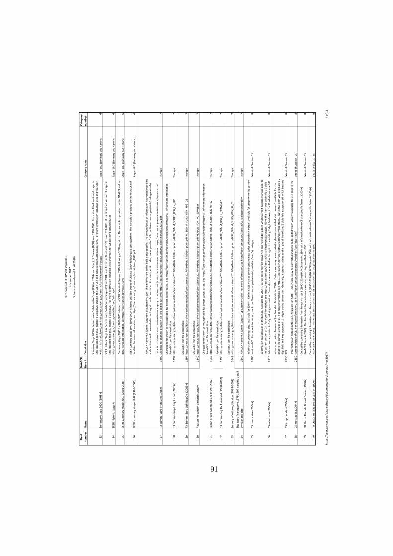
Dict

iona

ry o

f SEE

R*St

at V

aria

bles

N

ovem

ber 2

017

Sub

mis

sion

(rel

ease

d Ap

ril 2

018)

http

s://

seer

.can

cer.g

ov/d

ata-

soft

war

e/do

cum

enta

tion/

seer

stat

/nov

2017

/4

of 1

1

Fiel

d nu

mbe

rN

ame

NAA

CCR

Item

#D

escr

iptio

nCa

tego

ry n

ame

Cate

gory

nu

mbe

r

53Su

mm

ary

stag

e 20

00 (1

998+

)

Sum

mar

y St

age

2000

is d

eriv

ed fr

om C

olla

bora

tive

Stag

e (C

S) fo

r 200

4+ a

nd E

xten

t of D

iseas

e (E

OD)

from

199

8-20

03.

It is

a sim

plifi

ed v

ersio

n of

stag

e: in

sit

u, lo

caliz

ed, r

egio

nal,

dist

ant,

& u

nkno

wn.

Use

d in

the

SEER

CSR

and

mor

e re

cent

SEE

R pu

blic

atio

ns.

For m

ore

info

rmat

ion

incl

udin

g sit

es a

nd y

ears

for

whi

ch it

isn'

t cal

cula

ted,

see

http

s://

seer

.can

cer.g

ov/s

eers

tat/

varia

bles

/see

r/lrd

-sta

ge/

Stag

e - L

RD (S

umm

ary

and

Hist

oric

)6

54SE

ER h

isto

ric st

age

A

SEER

Hist

oric

Sta

ge A

is D

eriv

ed fr

om C

olla

bora

tive

Stag

e (C

S) fo

r 200

4+ a

nd E

xten

t of D

iseas

e (E

OD)

from

197

3-20

03.

It is

a sim

plifi

ed v

ersio

n of

stag

e: in

sit

u, lo

caliz

ed, r

egio

nal,

dist

ant,

& u

nkno

wn.

For

mor

e in

form

atio

n in

clud

ing

sites

and

yea

rs fo

r whi

ch it

isn'

t cal

cula

ted,

see

http

s://

seer

.can

cer.g

ov/s

eers

tat/

varia

bles

/see

r/lrd

-sta

ge/

Stag

e - L

RD (S

umm

ary

and

Hist

oric

)6

55SE

ER su

mm

ary

stag

e 20

00 (2

001-

2003

)

Sum

mar

y St

age

2000

for 2

001-

2003

is b

ased

on

SEER

Ext

ent o

f Dise

ase

(EO

D) fo

llow

ing

a SE

ER a

lgor

ithm

. Th

is va

riabl

e is

prov

ided

on

the

NAA

CCR

call

for

data

. For

mor

e in

form

atio

n, se

e ht

tps:

//se

er.c

ance

r.gov

/too

ls/ss

m/

Stag

e - L

RD (S

umm

ary

and

Hist

oric

)6

56SE

ER su

mm

ary

stag

e 19

77 (1

995-

2000

)

SEER

sum

mar

y st

age

1977

(199

5-20

00) i

s bas

ed o

n SE

ER E

xten

t of D

iseas

e (E

OD)

follo

win

g a

SEER

alg

orith

m.

This

varia

ble

is pr

ovid

ed o

n th

e N

AACC

R ca

ll fo

r dat

a. F

or m

ore

info

rmat

ion,

see

http

s://

seer

.can

cer.g

ov/m

anua

ls/hi

stor

ic/s

sm_1

977.

pdf

Stag

e - L

RD (S

umm

ary

and

Hist

oric

)6

57RX

Sum

m--S

urg

Prim

Site

(199

8+)

1290

NAA

CCR

Nam

e=RX

Sum

m--S

urg

Prim

Site

, Ite

m #

=129

0. T

he in

form

atio

n in

this

field

is si

te-s

peci

fic.

The

amou

nt/d

etai

l of i

nfor

mat

ion

has v

arie

d ov

er ti

me

and

caut

ion

shou

ld b

e us

ed w

hen

look

ing

at tr

ends

ove

r tim

e.

For s

ite-s

peci

fic c

odes

, see

App

endi

x C

of h

ttps

://s

eer.c

ance

r.gov

/too

ls/co

ding

man

uals/

Data

for 1

998-

2002

are

con

vert

ed fr

om S

urge

ry o

f prim

ary

site

(199

8-20

02),

docu

men

ted

here

: htt

ps:/

/see

r.can

cer.g

ov/m

anua

ls/hi

stor

ic/A

ppen

dC.p

df.

See

here

for c

hang

es b

etw

een

the

two

codi

ng sy

stem

s: h

ttps

://s

eer.c

ance

r.gov

/too

ls/SE

ER20

03.c

ode.

chan

ges.

1223

02.p

dfTh

erap

y7

58RX

Sum

m--S

cope

Reg

LN

Sur

(200

3+)

1292

Chan

ged

to U

nkno

wn

or n

ot a

pplic

able

for b

reas

t can

cer c

ases

. Se

e ht

tps:

//se

er.c

ance

r.gov

/see

rsta

t/va

riabl

es/s

eer/

regi

onal

_ln/

for m

ore

info

rmat

ion.

Se

e AS

CII t

ext f

ile d

escr

iptio

n:

http

s://

seer

.can

cer.g

ov/d

ata-

soft

war

e/do

cum

enta

tion/

seer

stat

/nov

2017

/Tex

tDat

a.Fi

leDe

scrip

tion.

pdf#

RX_S

UM

M_S

COPE

_REG

_LN

_SU

RTh

erap

y7

59RX

Sum

m--S

urg

Oth

Reg

/Dis

(200

3+)

1294

See

ASCI

I tex

t file

des

crip

tion:

ht

tps:

//se

er.c

ance

r.gov

/dat

a-so

ftw

are/

docu

men

tatio

n/se

erst

at/n

ov20

17/T

extD

ata.

File

Desc

riptio

n.pd

f#RX

_SU

MM

_SU

RG_O

TH_R

EG_D

ISTh

erap

y7

60Re

ason

no

canc

er-d

irect

ed su

rger

y13

40Se

e AS

CII t

ext f

ile d

escr

iptio

n:

http

s://

seer

.can

cer.g

ov/d

ata-

soft

war

e/do

cum

enta

tion/

seer

stat

/nov

2017

/Tex

tDat

a.Fi

leDe

scrip

tion.

pdf#

REAS

ON

_FO

R_N

O_S

URG

ERY

Ther

apy

7

61Sc

ope

of re

g ly

mph

nd

surg

(199

8-20

02)

1647

Chan

ged

to U

nkno

wn

or n

ot a

pplic

able

for b

reas

t can

cer c

ases

. Se

e ht

tps:

//se

er.c

ance

r.gov

/see

rsta

t/va

riabl

es/s

eer/

regi

onal

_ln/

for m

ore

info

rmat

ion.

Se

e AS

CII t

ext f

ile d

escr

iptio

n:

http

s://

seer

.can

cer.g

ov/d

ata-

soft

war

e/do

cum

enta

tion/

seer

stat

/nov

2017

/Tex

tDat

a.Fi

leDe

scrip

tion.

pdf#

RX_S

UM

M_S

COPE

_REG

_98_

02Th

erap

y7

62RX

Sum

m--R

eg L

N E

xam

ined

(199

8-20

02)

1296

See

ASCI

I tex

t file

des

crip

tion:

http

s://

seer

.can

cer.g

ov/d

ata-

soft

war

e/do

cum

enta

tion/

seer

stat

/nov

2017

/Tex

tDat

a.Fi

leDe

scrip

tion.

pdf#

RX_S

UM

M_R

EG_L

N_E

XAM

INED

Ther

apy

7

63Su

rger

y of

oth

reg/

dis s

ites (

1998

-200

2)16

48Se

e AS

CII t

ext f

ile d

escr

iptio

n:

http

s://

seer

.can

cer.g

ov/d

ata-

soft

war

e/do

cum

enta

tion/

seer

stat

/nov

2017

/Tex

tDat

a.Fi

leDe

scrip

tion.

pdf#

RX_S

UM

M_S

URG

_OTH

_98_

02Th

erap

y7

64Si

te sp

ecifi

c su

rger

y (1

973-

1997

var

ying

det

ail

by y

ear a

nd si

te)

1640

NAA

CCR

Nam

e=RX

Sum

m--S

urge

ry T

ype,

Item

#=1

640.

For

mor

e in

form

atio

n, se

e ht

tps:

//se

er.c

ance

r.gov

/see

rsta

t/va

riabl

es/s

eer/

surg

ery.

Ther

apy

7

65CS

tum

or si

ze (2

004+

)28

00In

form

atio

n on

tum

or si

ze.

Avai

labl

e fo

r 200

4+.

Ear

lier c

ases

may

be

conv

erte

d an

d ne

w c

odes

add

ed w

hich

wer

en't

avai

labl

e fo

r use

prio

r to

the

curr

ent

vers

ion

of C

S. F

or m

ore

info

rmat

ion,

see

http

s://

seer

.can

cer.g

ov/s

eers

tat/

varia

bles

/see

r/aj

cc-s

tage

/.

Exte

nt o

f Dise

ase

- CS

8

66CS

ext

ensi

on (2

004+

)28

10

Info

rmat

ion

on e

xten

sion

of th

e tu

mor

. Av

aila

ble

for 2

004+

. Ea

rlier

cas

es m

ay b

e co

nver

ted

and

new

cod

es a

dded

whi

ch w

eren

't av

aila

ble

for u

se p

rior t

o th

e cu

rren

t ver

sion

of C

S. F

or m

ore

info

rmat

ion,

see

http

s://

seer

.can

cer.g

ov/s

eers

tat/

varia

bles

/see

r/aj

cc-s

tage

/. N

ote:

this

item

was

orig

inal

ly a

2 d

igit

field

and

was

exp

ande

d to

3 d

igits

dur

ing

conv

ersio

n. G

ener

ally

, a ze

ro w

as a

dded

to th

e rig

ht o

f the

exi

stin

g 2

digi

t fie

ld e

xcep

t for

99

whi

ch b

ecam

e 99

9.Ex

tent

of D

iseas

e - C

S8

67CS

lym

ph n

odes

(200

4+)

2830

Info

rmat

ion

on in

volv

emen

t of l

ymph

nod

es. A

vaila

ble

for 2

004+

. Ea

rlier

cas

es m

ay b

e co

nver

ted

and

new

cod

es a

dded

whi

ch w

eren

't av

aila

ble

for u

se

prio

r to

the

curr

ent v

ersio

n of

CS.

For

mor

e in

form

atio

n, se

e ht

tps:

//se

er.c

ance

r.gov

/see

rsta

t/va

riabl

es/s

eer/

ajcc

-sta

ge/.

Not

e: th

is ite

m w

as o

rigin

ally

a 2

di

git f

ield

and

was

exp

ande

d to

3 d

igits

dur

ing

conv

ersio

n. G

ener

ally

, a ze

ro w

as a

dded

to th

e rig

ht o

f the

exi

stin

g 2

digi

t fie

ld e

xcep

t for

99

whi

ch b

ecam

e 99

9.Ex

tent

of D

iseas

e - C

S8

68CS

met

s at d

x (2

004+

)28

50 In

form

atio

n on

dist

ant m

etas

tasis

. Ava

ilabl

e fo

r 200

4+.

Earli

er c

ases

may

be

conv

erte

d an

d ne

w c

odes

add

ed w

hich

wer

en't

avai

labl

e fo

r use

prio

r to

the

curr

ent v

ersio

n of

CS.

For

mor

e in

form

atio

n, se

e ht

tps:

//se

er.c

ance

r.gov

/see

rsta

t/va

riabl

es/s

eer/

ajcc

-sta

ge/.

Ex

tent

of D

iseas

e - C

S8

69ER

Sta

tus R

ecod

e Br

east

Can

cer (

1990

+)Cr

eate

d by

com

bini

ng in

form

atio

n fr

om T

umor

mar

ker 1

(199

0-20

03) (

NAA

CCR

Item

#=1

150)

, with

info

rmat

ion

from

CS

site-

spec

ific

fact

or 1

(200

4+)

(NAA

CCR

Item

#=2

880)

. Th

is fie

ld is

bla

nk fo

r non

-bre

ast c

ases

and

cas

es d

iagn

osed

bef

ore

1990

.Ex

tent

of D

iseas

e - C

S8

70PR

Sta

tus R

ecod

e Br

east

Can

cer (

1990

+)Cr

eate

d by

com

bini

ng in

form

atio

n fr

om T

umor

mar

ker 2

(199

0-20

03) (

NAA

CCR

Item

#=1

150)

, with

info

rmat

ion

from

CS

site-

spec

ific

fact

or 2

(200

4+)

(NAA

CCR

Item

#=2

880)

. T

his f

ield

is b

lank

for n

on-b

reas

t cas

es a

nd c

ases

dia

gnos

ed b

efor

e 19

90.

Exte

nt o

f Dise

ase

- CS

8

91

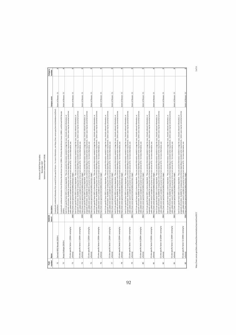
Dict

iona

ry o

f SEE

R*St

at V

aria

bles

N

ovem

ber 2

017

Sub

mis

sion

(rel

ease

d Ap

ril 2

018)

http

s://

seer

.can

cer.g

ov/d

ata-

soft

war

e/do

cum

enta

tion/

seer

stat

/nov

2017

/5

of 1

1

Fiel

d nu

mbe

rN

ame

NAA

CCR

Item

#D

escr

iptio

nCa

tego

ry n

ame

Cate

gory

nu

mbe

r

71De

rived

HER

2 Re

code

(201

0+)

Crea

ted

with

com

bine

d in

form

atio

n fr

om se

vera

l CS

site-

spec

ific

fact

ors.

For

mor

e in

form

atio

n, se

e ht

tps:

//se

er.c

ance

r.gov

/see

rsta

t/da

taba

ses/

ssf/

her2

-de

rived

.htm

l.Ex

tent

of D

iseas

e - C

S8

72Br

east

Sub

type

(201

0+)

Crea

ted

with

com

bine

d in

form

atio

n fr

om E

R St

atus

Rec

ode

Brea

st C

ance

r (19

90+)

, PR

Stat

us R

ecod

e Br

east

Can

cer (

1990

+), a

nd D

eriv

ed H

ER2

Reco

de

(201

0+).

Exte

nt o

f Dise

ase

- CS

8

73CS

site

-spe

cific

fact

or 1

(200

4+ v

aryi

ng b

y sc

hem

a)28

80

Each

CS

site-

spec

ific

fact

or (S

SF) i

s sch

ema

depe

nden

t. T

hey

can

prov

ide

info

rmat

ion

need

ed to

stag

e th

e ca

se, c

linic

ally

rele

vant

info

rmat

ion,

or

prog

nost

ic in

form

atio

n. A

vaila

ble

for v

aryi

ng y

ears

and

sche

mas

dep

endi

ng o

n st

anda

rd se

tter

requ

irem

ents

. Ea

rlier

cas

es m

ay b

e co

nver

ted

and

new

co

des a

dded

whi

ch w

eren

't av

aila

ble

for u

se p

rior t

o th

e cu

rren

t ver

sion

of C

S. F

or m

ore

info

rmat

ion,

see

http

s://

seer

.can

cer.g

ov/s

eers

tat/

varia

bles

/see

r/aj

cc-s

tage

/.

Exte

nt o

f Dise

ase

- CS

8

74CS

site

-spe

cific

fact

or 2

(200

4+ v

aryi

ng b

y sc

hem

a)28

90

Each

CS

site-

spec

ific

fact

or (S

SF) i

s sch

ema

depe

nden

t. T

hey

can

prov

ide

info

rmat

ion

need

ed to

stag

e th

e ca

se, c

linic

ally

rele

vant

info

rmat

ion,

or

prog

nost

ic in

form

atio

n. A

vaila

ble

for v

aryi

ng y

ears

and

sche

mas

dep

endi

ng o

n st

anda

rd se

tter

requ

irem

ents

. Ea

rlier

cas

es m

ay b

e co

nver

ted

and

new

co

des a

dded

whi

ch w

eren

't av

aila

ble

for u

se p

rior t

o th

e cu

rren

t ver

sion

of C

S. F

or m

ore

info

rmat

ion,

see

http

s://

seer

.can

cer.g

ov/s

eers

tat/

varia

bles

/see

r/aj

cc-s

tage

/.

Exte

nt o

f Dise

ase

- CS

8

75CS

site

-spe

cific

fact

or 3

(200

4+ v

aryi

ng b

y sc

hem

a)29

00

Each

CS

site-

spec

ific

fact

or (S

SF) i

s sch

ema

depe

nden

t. T

hey

can

prov

ide

info

rmat

ion

need

ed to

stag

e th

e ca

se, c

linic

ally

rele

vant

info

rmat

ion,

or

prog

nost

ic in

form

atio

n. A

vaila

ble

for v

aryi

ng y

ears

and

sche

mas

dep

endi

ng o

n st

anda

rd se

tter

requ

irem

ents

. Ea

rlier

cas

es m

ay b

e co

nver

ted

and

new

co

des a

dded

whi

ch w

eren

't av

aila

ble

for u

se p

rior t

o th

e cu

rren

t ver

sion

of C

S. F

or m

ore

info

rmat

ion,

see

http

s://

seer

.can

cer.g

ov/s

eers

tat/

varia

bles

/see

r/aj

cc-s

tage

/.

Exte

nt o

f Dise

ase

- CS

8

76CS

site

-spe

cific

fact

or 4

(200

4+ v

aryi

ng b

y sc

hem

a)29

10

Each

CS

site-

spec

ific

fact

or (S

SF) i

s sch

ema

depe

nden

t. T

hey

can

prov

ide

info

rmat

ion

need

ed to

stag

e th

e ca

se, c

linic

ally

rele

vant

info

rmat

ion,

or

prog

nost

ic in

form

atio

n. A

vaila

ble

for v

aryi

ng y

ears

and

sche

mas

dep

endi

ng o

n st

anda

rd se

tter

requ

irem

ents

. Ea

rlier

cas

es m

ay b

e co

nver

ted

and

new

co

des a

dded

whi

ch w

eren

't av

aila

ble

for u

se p

rior t

o th

e cu

rren

t ver

sion

of C

S. F

or m

ore

info

rmat

ion,

see

http

s://

seer

.can

cer.g

ov/s

eers

tat/

varia

bles

/see

r/aj

cc-s

tage

/.

Exte

nt o

f Dise

ase

- CS

8

77CS

site

-spe

cific

fact

or 5

(200

4+ v

aryi

ng b

y sc

hem

a)29

20

Each

CS

site-

spec

ific

fact

or (S

SF) i

s sch

ema

depe

nden

t. T

hey

can

prov

ide

info

rmat

ion

need

ed to

stag

e th

e ca

se, c

linic

ally

rele

vant

info

rmat

ion,

or

prog

nost

ic in

form

atio

n. A

vaila

ble

for v

aryi

ng y

ears

and

sche

mas

dep

endi

ng o

n st

anda

rd se

tter

requ

irem

ents

. Ea

rlier

cas

es m

ay b

e co

nver

ted

and

new

co

des a

dded

whi

ch w

eren

't av

aila

ble

for u

se p

rior t

o th

e cu

rren

t ver

sion

of C

S. F

or m

ore

info

rmat

ion,

see

http

s://

seer

.can

cer.g

ov/s

eers

tat/

varia

bles

/see

r/aj

cc-s

tage

/.

Exte

nt o

f Dise

ase

- CS

8

78CS

site

-spe

cific

fact

or 6

(200

4+ v

aryi

ng b

y sc

hem

a)29

30

Each

CS

site-

spec

ific

fact

or (S

SF) i

s sch

ema

depe

nden

t. T

hey

can

prov

ide

info

rmat

ion

need

ed to

stag

e th

e ca

se, c

linic

ally

rele

vant

info

rmat

ion,

or

prog

nost

ic in

form

atio

n. A

vaila

ble

for v

aryi

ng y

ears

and

sche

mas

dep

endi

ng o

n st

anda

rd se

tter

requ

irem

ents

. Ea

rlier

cas

es m

ay b

e co

nver

ted

and

new

co

des a

dded

whi

ch w

eren

't av

aila

ble

for u

se p

rior t

o th

e cu

rren

t ver

sion

of C

S. F

or m

ore

info

rmat

ion,

see

http

s://

seer

.can

cer.g

ov/s

eers

tat/

varia

bles

/see

r/aj

cc-s

tage

/.

Exte

nt o

f Dise

ase

- CS

8

79CS

site

-spe

cific

fact

or 7

(200

4+ v

aryi

ng b

y sc

hem

a)28

61

Each

CS

site-

spec

ific

fact

or (S

SF) i

s sch

ema

depe

nden

t. T

hey

can

prov

ide

info

rmat

ion

need

ed to

stag

e th

e ca

se, c

linic

ally

rele

vant

info

rmat

ion,

or

prog

nost

ic in

form

atio

n. A

vaila

ble

for v

aryi

ng y

ears

and

sche

mas

dep

endi

ng o

n st

anda

rd se

tter

requ

irem

ents

. Ea

rlier

cas

es m

ay b

e co

nver

ted

and

new

co

des a

dded

whi

ch w

eren

't av

aila

ble

for u

se p

rior t

o th

e cu

rren

t ver

sion

of C

S. F

or m

ore

info

rmat

ion,

see

http

s://

seer

.can

cer.g

ov/s

eers

tat/

varia

bles

/see

r/aj

cc-s

tage

/.

Exte

nt o

f Dise

ase

- CS

8

80CS

site

-spe

cific

fact

or 8

(200

4+ v

aryi

ng b

y sc

hem

a)28

62

Each

CS

site-

spec

ific

fact

or (S

SF) i

s sch

ema

depe

nden

t. T

hey

can

prov

ide

info

rmat

ion

need

ed to

stag

e th

e ca

se, c

linic

ally

rele

vant

info

rmat

ion,

or

prog

nost

ic in

form

atio

n. A

vaila

ble

for v

aryi

ng y

ears

and

sche

mas

dep

endi

ng o

n st

anda

rd se

tter

requ

irem

ents

. Ea

rlier

cas

es m

ay b

e co

nver

ted

and

new

co

des a

dded

whi

ch w

eren

't av

aila

ble

for u

se p

rior t

o th

e cu

rren

t ver

sion

of C

S. F

or m

ore

info

rmat

ion,

see

http

s://

seer

.can

cer.g

ov/s

eers

tat/

varia

bles

/see

r/aj

cc-s

tage

/.

Exte

nt o

f Dise

ase

- CS

8

81CS

site

-spe

cific

fact

or 9

(200

4+ v

aryi

ng b

y sc

hem

a)28

63

Each

CS

site-

spec

ific

fact

or (S

SF) i

s sch

ema

depe

nden

t. T

hey

can

prov

ide

info

rmat

ion

need

ed to

stag

e th

e ca

se, c

linic

ally

rele

vant

info

rmat

ion,

or

prog

nost

ic in

form

atio

n. A

vaila

ble

for v

aryi

ng y

ears

and

sche

mas

dep

endi

ng o

n st

anda

rd se

tter

requ

irem

ents

. Ea

rlier

cas

es m

ay b

e co

nver

ted

and

new

co

des a

dded

whi

ch w

eren

't av

aila

ble

for u

se p

rior t

o th

e cu

rren

t ver

sion

of C

S. F

or m

ore

info

rmat

ion,

see

http

s://

seer

.can

cer.g

ov/s

eers

tat/

varia

bles

/see

r/aj

cc-s

tage

/.

Exte

nt o

f Dise

ase

- CS

8

82CS

site

-spe

cific

fact

or 1

0 (2

004+

var

ying

by

sche

ma)

2864

Each

CS

site-

spec

ific

fact

or (S

SF) i

s sch

ema

depe

nden

t. T

hey

can

prov

ide

info

rmat

ion

need

ed to

stag

e th

e ca

se, c

linic

ally

rele

vant

info

rmat

ion,

or

prog

nost

ic in

form

atio

n. A

vaila

ble

for v

aryi

ng y

ears

and

sche

mas

dep

endi

ng o

n st

anda

rd se

tter

requ

irem

ents

. Ea

rlier

cas

es m

ay b

e co

nver

ted

and

new

co

des a

dded

whi

ch w

eren

't av

aila

ble

for u

se p

rior t

o th

e cu

rren

t ver

sion

of C

S. F

or m

ore

info

rmat

ion,

see

http

s://

seer

.can

cer.g

ov/s

eers

tat/

varia

bles

/see

r/aj

cc-s

tage

/.

Exte

nt o

f Dise

ase

- CS

8

83CS

site

-spe

cific

fact

or 1

1 (2

004+

var

ying

by

sche

ma)

2865

Each

CS

site-

spec

ific

fact

or (S

SF) i

s sch

ema

depe

nden

t. T

hey

can

prov

ide

info

rmat

ion

need

ed to

stag

e th

e ca

se, c

linic

ally

rele

vant

info

rmat

ion,

or

prog

nost

ic in

form

atio

n. A

vaila

ble

for v

aryi

ng y

ears

and

sche

mas

dep

endi

ng o

n st

anda

rd se

tter

requ

irem

ents

. Ea

rlier

cas

es m

ay b

e co

nver

ted

and

new

co

des a

dded

whi

ch w

eren

't av

aila

ble

for u

se p

rior t

o th

e cu

rren

t ver

sion

of C

S. F

or m

ore

info

rmat

ion,

see

http

s://

seer

.can

cer.g

ov/s

eers

tat/

varia

bles

/see

r/aj

cc-s

tage

/.

Exte

nt o

f Dise

ase

- CS

8

84CS

site

-spe

cific

fact

or 1

2 (2

004+

var

ying

by

sche

ma)

2866

Each

CS

site-

spec

ific

fact

or (S

SF) i

s sch

ema

depe

nden

t. T

hey

can

prov

ide

info

rmat

ion

need

ed to

stag

e th

e ca

se, c

linic

ally

rele

vant

info

rmat

ion,

or

prog

nost

ic in

form

atio

n. A

vaila

ble

for v

aryi

ng y

ears

and

sche

mas

dep

endi

ng o

n st

anda

rd se

tter

requ

irem

ents

. Ea

rlier

cas

es m

ay b

e co

nver

ted

and

new

co

des a

dded

whi

ch w

eren

't av

aila

ble

for u

se p

rior t

o th

e cu

rren

t ver

sion

of C

S. F

or m

ore

info

rmat

ion,

see

http

s://

seer

.can

cer.g

ov/s

eers

tat/

varia

bles

/see

r/aj

cc-s

tage

/.

Exte

nt o

f Dise

ase

- CS

8

92

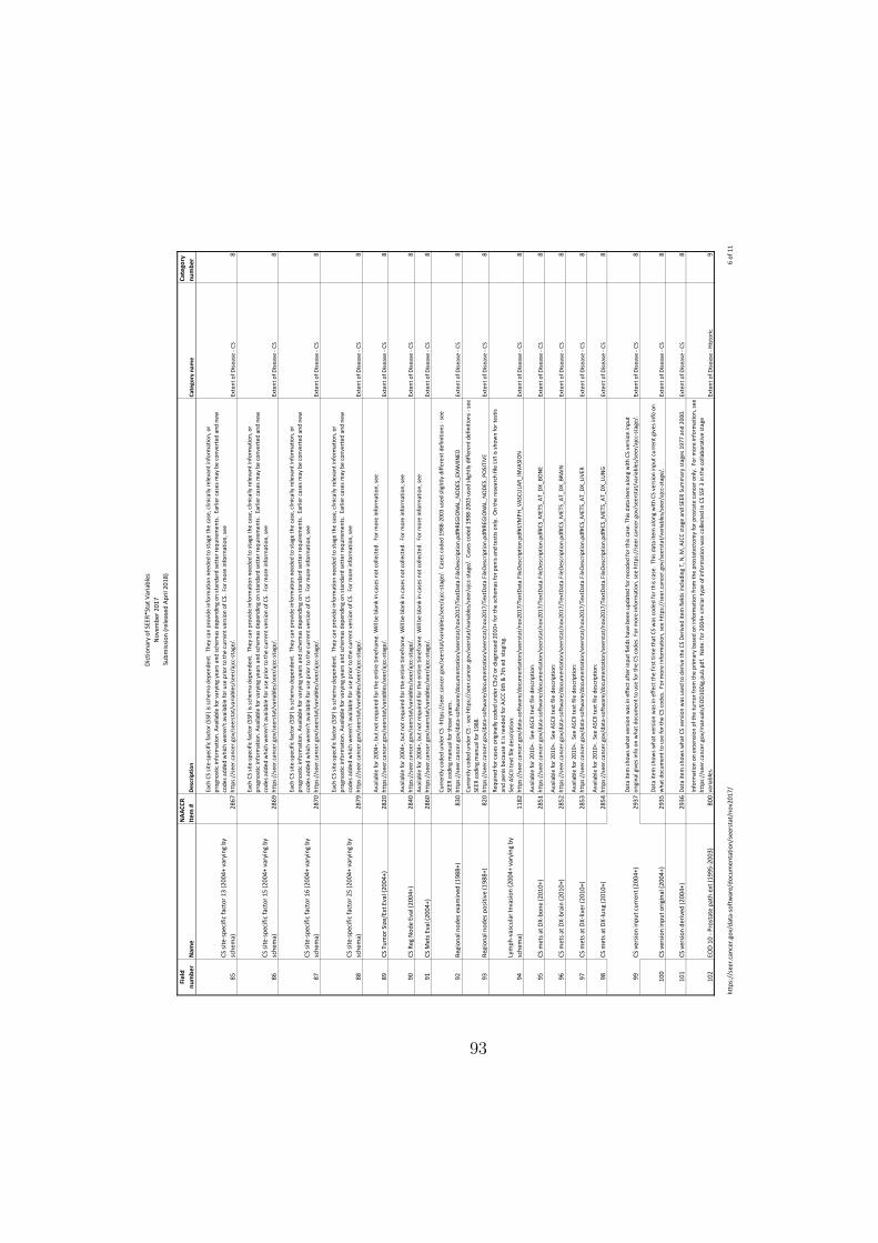
Dict

iona

ry o

f SEE

R*St

at V

aria

bles

N

ovem

ber 2

017

Sub

mis

sion

(rel

ease

d Ap

ril 2

018)

http

s://

seer

.can

cer.g

ov/d

ata-

soft

war

e/do

cum

enta

tion/

seer

stat

/nov

2017

/6

of 1

1

Fiel

d nu

mbe

rN

ame

NAA

CCR

Item

#D

escr

iptio

nCa

tego

ry n

ame

Cate

gory

nu

mbe

r

85CS

site

-spe

cific

fact

or 1

3 (2

004+

var

ying

by

sche

ma)

2867

Each

CS

site-

spec

ific

fact

or (S

SF) i

s sch

ema

depe

nden

t. T

hey

can

prov

ide

info

rmat

ion

need

ed to

stag

e th

e ca

se, c

linic

ally

rele

vant

info

rmat

ion,

or

prog

nost

ic in

form

atio

n. A

vaila

ble

for v

aryi

ng y

ears

and

sche

mas

dep

endi

ng o

n st

anda

rd se

tter

requ

irem

ents

. Ea

rlier

cas

es m

ay b

e co

nver

ted

and

new

co

des a

dded

whi

ch w

eren

't av

aila

ble

for u

se p

rior t

o th

e cu

rren

t ver

sion

of C

S. F

or m

ore

info

rmat

ion,

see

http

s://

seer

.can

cer.g

ov/s

eers

tat/

varia

bles

/see

r/aj

cc-s

tage

/.

Exte

nt o

f Dise

ase

- CS

8

86CS

site

-spe

cific

fact

or 1

5 (2

004+

var

ying

by

sche

ma)

2869

Each

CS

site-

spec

ific

fact

or (S

SF) i

s sch

ema

depe

nden

t. T

hey

can

prov

ide

info

rmat

ion

need

ed to

stag

e th

e ca

se, c

linic

ally

rele

vant

info

rmat

ion,

or

prog

nost

ic in

form

atio

n. A

vaila

ble

for v

aryi

ng y

ears

and

sche

mas

dep

endi

ng o

n st

anda

rd se

tter

requ

irem

ents

. Ea

rlier

cas

es m

ay b

e co

nver

ted

and

new

co

des a

dded

whi

ch w

eren

't av

aila

ble

for u

se p

rior t

o th

e cu

rren

t ver

sion

of C

S. F

or m

ore

info

rmat

ion,

see

http

s://

seer

.can

cer.g

ov/s

eers

tat/

varia

bles

/see

r/aj

cc-s

tage

/.

Exte

nt o

f Dise

ase

- CS

8

87CS

site

-spe

cific

fact

or 1

6 (2

004+

var

ying

by

sche

ma)

2870

Each

CS

site-

spec

ific

fact

or (S

SF) i

s sch

ema

depe

nden

t. T

hey

can

prov

ide

info

rmat

ion

need

ed to

stag

e th

e ca

se, c

linic

ally

rele

vant

info

rmat

ion,

or

prog

nost

ic in

form

atio

n. A

vaila

ble

for v

aryi

ng y

ears

and

sche

mas

dep

endi

ng o

n st

anda

rd se

tter

requ

irem

ents

. Ea

rlier

cas

es m

ay b

e co

nver

ted

and

new

co

des a

dded

whi

ch w

eren

't av

aila

ble

for u

se p

rior t

o th

e cu

rren

t ver

sion

of C

S. F

or m

ore

info

rmat

ion,

see

http

s://

seer

.can

cer.g

ov/s

eers

tat/

varia

bles

/see

r/aj

cc-s

tage

/.

Exte

nt o

f Dise

ase

- CS

8

88CS

site

-spe

cific

fact

or 2

5 (2

004+

var

ying

by

sche

ma)

2879

Each

CS

site-

spec

ific

fact

or (S

SF) i

s sch

ema

depe

nden

t. T

hey

can

prov

ide

info

rmat

ion

need

ed to

stag

e th

e ca

se, c

linic

ally

rele

vant

info

rmat

ion,

or

prog

nost

ic in

form

atio

n. A

vaila

ble

for v

aryi

ng y

ears

and

sche

mas

dep

endi

ng o

n st

anda

rd se

tter

requ

irem

ents

. Ea

rlier

cas

es m

ay b

e co

nver

ted

and

new

co

des a

dded

whi

ch w

eren

't av

aila

ble

for u

se p

rior t

o th

e cu

rren

t ver

sion

of C

S. F

or m

ore

info

rmat

ion,

see

http

s://

seer

.can

cer.g

ov/s

eers

tat/

varia

bles

/see

r/aj

cc-s

tage

/.

Exte

nt o

f Dise

ase

- CS

8

89CS

Tum

or S

ize/

Ext E

val (

2004

+)28

20Av

aila

ble

for 2

004+

, but

not

requ

ired

for t

he e

ntire

tim

efra

me.

Will

be

blan

k in

cas

es n

ot c

olle

cted

. Fo

r mor

e in

form

atio

n, se

e ht

tps:

//se

er.c

ance

r.gov

/see

rsta

t/va

riabl

es/s

eer/

ajcc

-sta

ge/.

Exte

nt o

f Dise

ase

- CS

8

90CS

Reg

Nod

e Ev

al (2

004+

)28

40Av

aila

ble

for 2

004+

, but

not

requ

ired

for t

he e

ntire

tim

efra

me.

Will

be

blan

k in

cas

es n

ot c

olle

cted

. Fo

r mor

e in

form

atio

n, se

e ht

tps:

//se

er.c

ance

r.gov

/see

rsta

t/va

riabl

es/s

eer/

ajcc

-sta

ge/.

Exte

nt o

f Dise

ase

- CS

8

91CS

Met

s Eva

l (20

04+)

2860

Avai

labl

e fo

r 200

4+, b

ut n

ot re

quire

d fo

r the

ent

ire ti

mef

ram

e. W

ill b

e bl

ank

in c

ases

not

col

lect

ed.

For m

ore

info

rmat

ion,

see

http

s://

seer

.can

cer.g

ov/s

eers

tat/

varia

bles

/see

r/aj

cc-s

tage

/.Ex

tent

of D

iseas

e - C

S8

92Re

gion

al n

odes

exa

min

ed (1

988+

)83

0

Curr

ently

cod

ed u

nder

CS

-htt

ps:/

/see

r.can

cer.g

ov/s

eers

tat/

varia

bles

/see

r/aj

cc-s

tage

/. C

ases

cod

ed 1

988-

2003

use

d sli

ghtly

diff

eren

t def

initi

ons -

see

SEER

cod

ing

man

ual f

or th

ose

year

s.

http

s://

seer

.can

cer.g

ov/d

ata-

soft

war

e/do

cum

enta

tion/

seer

stat

/nov

2017

/Tex

tDat

a.Fi

leDe

scrip

tion.

pdf#

REG

ION

AL_N

ODE

S_EX

AMIN

EDEx

tent

of D

iseas

e - C

S8

93Re

gion

al n

odes

pos

itive

(198

8+)

820

Curr

ently

cod

ed u

nder

CS

- see

htt

ps:/

/see

r.can

cer.g

ov/s

eers

tat/

varia

bles

/see

r/aj

cc-s

tage

/. C

ases

cod

ed 1

988-

2003

use

d sli

ghtly

diff

eren

t def

initi

ons -

see

SEER

cod

ing

man

ual f

or 1

988.

ht

tps:

//se

er.c

ance

r.gov

/dat

a-so

ftw

are/

docu

men

tatio

n/se

erst

at/n

ov20

17/T

extD

ata.

File

Desc

riptio

n.pd

f#RE

GIO

NAL

_NO

DES_

POSI

TIVE

Exte

nt o

f Dise

ase

- CS

8

94Ly

mph

-vas

cula

r Inv

asio

n (2

004+

var

ying

by

sche

ma)

1182

Requ

ired

for c

ases

orig

inal

ly c

oded

und

er C

Sv2

or d

iagn

osed

201

0+ fo

r the

sche

mas

for p

enis

and

test

is on

ly.

On

the

rese

arch

file

LVI

is sh

own

for t

estis

an

d pe

nis b

ecau

se it

is n

eede

d fo

r AJC

C 6t

h &

7th

ed

stag

ing.

Se

e AS

CII t

ext f

ile d

escr

iptio

n:

http

s://

seer

.can

cer.g

ov/d

ata-

soft

war

e/do

cum

enta

tion/

seer

stat

/nov

2017

/Tex

tDat

a.Fi

leDe

scrip

tion.

pdf#

LYM

PH_V

ASCU

LAR_

INVA

SIO

NEx

tent

of D

iseas

e - C

S8

95CS

met

s at D

X-bo

ne (2

010+

)28

51Av

aila

ble

for 2

010+

. Se

e AS

CII t

ext f

ile d

escr

iptio

n:

http

s://

seer

.can

cer.g

ov/d

ata-

soft

war

e/do

cum

enta

tion/

seer

stat

/nov

2017

/Tex

tDat

a.Fi

leDe

scrip

tion.

pdf#

CS_M

ETS_

AT_D

X_BO

NE

Exte

nt o

f Dise

ase

- CS

8

96CS

met

s at D

X-br

ain

(201

0+)

2852

Avai

labl

e fo

r 201

0+.

See

ASCI

I tex

t file

des

crip

tion:

ht

tps:

//se

er.c

ance

r.gov

/dat

a-so

ftw

are/

docu

men

tatio

n/se

erst

at/n

ov20

17/T

extD

ata.

File

Desc

riptio

n.pd

f#CS

_MET

S_AT

_DX_

BRAI

NEx

tent

of D

iseas

e - C

S8

97CS

met

s at D

X-liv

er (2

010+

)28

53Av

aila

ble

for 2

010+

. Se

e AS

CII t

ext f

ile d

escr

iptio

n:

http

s://

seer

.can

cer.g

ov/d

ata-

soft

war

e/do

cum

enta

tion/

seer

stat

/nov

2017

/Tex

tDat

a.Fi

leDe

scrip

tion.

pdf#

CS_M

ETS_

AT_D

X_LI

VER

Exte

nt o

f Dise

ase

- CS

8

98CS

met

s at D

X-lu

ng (2

010+

)28

54Av

aila

ble

for 2

010+

. Se

e AS

CII t

ext f

ile d

escr

iptio

n:

http

s://

seer

.can

cer.g

ov/d

ata-

soft

war

e/do

cum

enta

tion/

seer

stat

/nov

2017

/Tex

tDat

a.Fi

leDe

scrip

tion.

pdf#

CS_M

ETS_

AT_D

X_LU

NG

Exte

nt o

f Dise

ase

- CS

8

99CS

ver

sion

inpu

t cur

rent

(200

4+)

2937

Data

item

show

s wha

t ver

sion

was

in e

ffect

aft

er in

put f

ield

s hav

e be

en u

pdat

ed fo

r rec

oded

for t

his c

ase.

Thi

s dat

a ite

m a

long

with

CS

vers

ion

inpu

t or

igin

al g

ives

info

on

wha

t doc

umen

t to

use

for t

he C

S co

des.

For

mor

e in

form

atio

n, se

e ht

tps:

//se

er.c

ance

r.gov

/see

rsta

t/va

riabl

es/s

eer/

ajcc

-sta

ge/.

Ex

tent

of D

iseas

e - C

S8

100

CS v

ersi

on in

put o

rigin

al (2

004+

)29

35Da

ta it

em sh

ows w

hat v

ersio

n w

as in

effe

ct th

e fir

st ti

me

that

CS

was

cod

ed fo

r thi

s cas

e. T

his d

ata

item

alo

ng w

ith C

S ve

rsio

n in

put c

urre

nt g

ives

info

on

wha

t doc

umen

t to

use

for t

he C

S co

des.

For

mor

e in

form

atio

n, se

e ht

tps:

//se

er.c

ance

r.gov

/see

rsta

t/va

riabl

es/s

eer/

ajcc

-sta

ge/.

Ex

tent

of D

iseas

e - C

S8

101

CS v

ersi

on d

eriv

ed (2

004+

)29

36Da

ta it

em sh

ows w

hat C

S ve

rsio

n w

as u

sed

to d

eriv

e th

e CS

Der

ived

item

fiel

ds in

clud

ing

T, N

, M, A

JCC

stag

e an

d SE

ER S

umm

ary

stag

es 1

977

and

2000

.Ex

tent

of D

iseas

e - C

S8

102

EOD

10 -

Pros

tate

pat

h ex

t (19

95-2

003)

800

Info

rmat

ion

on e

xten

sion

of th

e tu

mor

from

the

prim

ary

base

d on

info

rmat

ion

from

the

pros

tate

ctom

y fo

r pro

stat

e ca

ncer

onl

y. F

or m

ore

info

rmat

ion,

see

http

s://

seer

.can

cer.g

ov/m

anua

ls/EO

D10D

ig.p

ub.p

df.

Not

e: fo

r 200

4+ si

mila

r typ

e of

info

rmat

ion

was

col

lect

ed in

CS

SSF

3 in

the

colla

bora

tive

stag

e va

riabl

es.

Exte

nt o

f Dise

ase

- Hist

oric

9

93

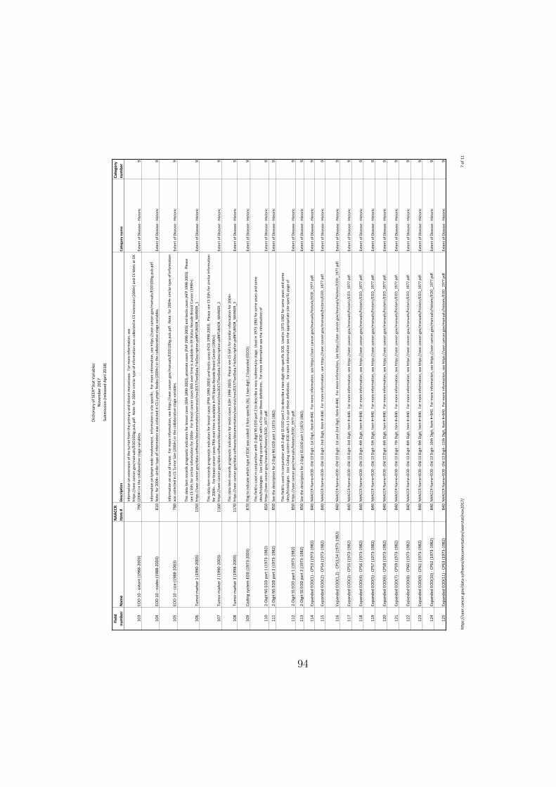
Dict

iona

ry o

f SEE

R*St

at V

aria

bles

N

ovem

ber 2

017

Sub

mis

sion

(rel

ease

d Ap

ril 2

018)

http

s://

seer

.can

cer.g

ov/d

ata-

soft

war

e/do

cum

enta

tion/

seer

stat

/nov

2017

/7

of 1

1

Fiel

d nu

mbe

rN

ame

NAA

CCR

Item

#D

escr

iptio

nCa

tego

ry n

ame

Cate

gory

nu

mbe

r

103

EOD

10 -

exte

nt (1

988-

2003

)79

0

Info

rmat

ion

on e

xten

sion

of th

e tu

mor

from

the

prim

ary

and

dist

ant m

etas

tase

s. F

or m

ore

info

rmat

ion,

see

http

s://

seer

.can

cer.g

ov/m

anua

ls/EO

D10D

ig.p

ub.p

df.

Not

e: fo

r 200

4+ si

mila

r typ

e of

info

rmat

ion

was

col

lect

ed in

CS

exte

nsio

n (2

004+

) and

CS

Met

s at D

X (2

004+

) in

the

colla

bora

tive

stag

e va

riabl

es.

Exte

nt o

f Dise

ase

- Hist

oric

9

104

EOD

10 -

node

s (19

88-2

003)

810

Info

rmat

ion

on ly

mph

nod

e in

volv

emen

t. In

form

atio

n is

site-

spec

ific.

For

mor

e in

form

atio

n, se

e ht

tps:

//se

er.c

ance

r.gov

/man

uals/

EOD1

0Dig

.pub

.pdf

. N

ote:

for 2

004+

sim

ilar t

ype

of in

form

atio

n w

as c

olle

cted

in C

S Ly

mph

Nod

es (2

004+

) in

the

colla

bora

tive

stag

e va

riabl

es.

Exte

nt o

f Dise

ase

- Hist

oric

9

105

EOD

10 -

size

(198

8-20

03)

780

Info

rmat

ion

on si

ze o

f tum

or.

For m

ore

info

rmat

ion,

see

http

s://

seer

.can

cer.g

ov/m

anua

ls/EO

D10D

ig.p

ub.p

df.

Not

e: fo

r 200

4+ si

mila

r typ

e of

info

rmat

ion

was

col

lect

ed in

CS

Tum

or S

ize (2

004+

) in

the

colla

bora

tive

stag

e va

riabl

es.

Exte

nt o

f Dise

ase

- Hist

oric

9

106

Tum

or m

arke

r 1 (1

990-

2003

)11

50

This

data

item

reco

rds p

rogn

ostic

indi

cato

rs fo

r bre

ast c

ases

(ERA

199

0-20

03),

pros

tate

cas

es (P

AP 1

998-

2003

) and

test

is ca

ses (

AFP

1998

-200

3).

Plea

se

see

CS S

SFs f

or si

mila

r inf

orm

atio

n fo

r 200

4+.

For b

reas

t can

cer c

ases

ERA

ove

r tim

e is

avai

labl

e in

ER

Stat

us R

ecod

e Br

east

Can

cer (

1990

+).

http

s://

seer

.can

cer.g

ov/d

ata-

soft

war

e/do

cum

enta

tion/

seer

stat

/nov

2017

/Tex

tDat

a.Fi

leDe

scrip

tion.

pdf#

TUM

OR_

MAR

KER_

1Ex

tent

of D

iseas

e - H

istor

ic9

107

Tum

or m

arke

r 2 (1

990-

2003

)11

60

This

data

item

reco

rds p

rogn

ostic

indi

cato

rs fo

r bre

ast c

ases

(PRA

199

0-20

03) a

nd te

stis

case

s (hC

G 1

998-

2003

). P

leas

e se

e CS

SSF

s for

sim

ilar i

nfor

mat

ion

for 2

004+

. Fo

r bre

ast c

ance

r cas

es P

RA o

ver t

ime

is av

aila

ble

in P

R St

atus

Rec

ode

Brea

st C

ance

r (19

90+)

. ht

tps:

//se

er.c

ance

r.gov

/dat

a-so

ftw

are/

docu

men

tatio

n/se

erst

at/n

ov20

17/T

extD

ata.

File

Desc

riptio

n.pd

f#TU

MO

R_M

ARKE

R_2

Exte

nt o

f Dise

ase

- Hist

oric

9

108

Tum

or m

arke

r 3 (1

998-

2003

)11

70Th

is da

ta it

em re

cord

s pro

gnos

tic in

dica

tors

for t

estis

cas

es (L

DH 1

998-

2003

). P

leas

e se

e CS

SSF

s for

sim

ilar i

nfor

mat

ion

for 2

004+

. ht

tps:

//se

er.c

ance

r.gov

/dat

a-so

ftw

are/

docu

men

tatio

n/se

erst

at/n

ov20

17/T

extD

ata.

File

Desc

riptio

n.pd

f#TU

MO

R_M

ARKE

R_3

Exte

nt o

f Dise

ase

- Hist

oric

9

109

Codi

ng sy

stem

-EO

D (1

973-

2003

)87

0Fl

ag to

indi

cate

whi

ch ty

pe o

f EO

D w

as c

oded

: 0 N

on-s

peci

fic (N

); 1

two-

digi

t; 2

Expa

nded

(EEO

D)Ex

tent

of D

iseas

e - H

istor

ic9

110

2-Di

git N

S EO

D pa

rt 1

(197

3-19

82)

850

This

field

is u

sed

in c

onju

nctio

n w

ith 2

-dig

it N

S EO

D pa

rt 2

to d

escr

ibe

a ve

ry ru

dim

enta

ry st

age.

Use

d in

197

3-19

82 fo

r som

e ye

ars a

nd so

me

sites

/hist

olog

ies.

Use

Cod

ing

syst

em-E

OD

with

a 0

to u

se th

ese

defin

ition

s. F

or m

ore

info

rmat

ion

see

the

intr

oduc

tion

of

http

s://

seer

.can

cer.g

ov/m

anua

ls/hi

stor

ic/E

OD_

1977

.pdf

.Ex

tent

of D

iseas

e - H

istor

ic9

111

2-Di

git N

S EO

D pa

rt 2

(197

3-19

82)

850

See

the

desc

riptio

n fo

r 2-D

igit

NS

EOD

part

1 (1

973-

1982

).Ex

tent

of D

iseas

e - H

istor

ic9

112

2-Di

git S

S EO

D pa

rt 1

(197

3-19

82)

850

This

field

is u

sed

in c

onju

nctio

n w

ith 2

-dig

it SS

EO

D pa

rt 2

to d

escr

ibe

a tw

o-di

git s

ite-s

peci

fic E

OD.

Use

d in

197

3-19

82 fo

r som

e ye

ars a

nd so

me

sites

/hist

olog

ies.

Use

Cod

ing

syst

em-E

OD

with

a 1

to u

se th

ese

defin

ition

s. F

or m

ore

info

rmat

ion

see

the

appr

opria

te si

te-s

peci

fic p

age

of

http

s://

seer

.can

cer.g

ov/m

anua

ls/hi

stor

ic/E

OD_

1977

.pdf

.Ex

tent

of D

iseas

e - H

istor

ic9

113

2-Di

git S

S EO

D pa

rt 2

(197

3-19

82)

850

See

the

desc

riptio

n fo

r 2-D

igit

SS E

OD

part

1 (1

973-

1982

).Ex

tent

of D

iseas

e - H

istor

ic9

114

Expa

nded

EO

D(1)

- CP

53 (1

973-

1982

)84

0N

AACC

R N

ame=

EOD-

-Old

13

Digi

t--1

st D

igit,

Item

#=8

40.

For m

ore

info

rmat

ion,

see

http

s://

seer

.can

cer.g

ov/m

anua

ls/hi

stor

ic/E

OD_

1977

.pdf

.Ex

tent

of D

iseas

e - H

istor

ic9

115

Expa

nded

EO

D(2)

- CP

54 (1

973-

1982

)84

0N

AACC

R N

ame=

EOD-

-Old

13

Digi

t--2

nd D

igit,

Item

#=8

40.

For m

ore

info

rmat

ion,

see

http

s://

seer

.can

cer.g

ov/m

anua

ls/hi

stor

ic/E

OD_

1977

.pdf

.Ex

tent

of D

iseas

e - H

istor

ic9

116

Expa

nded

EO

D(1,

2) -

CP53

,54

(197

3-19

82)

840

NAA

CCR

Nam

e=EO

D--O

ld 1

3 Di

git-

-1st

and

2nd

Dig

it, It

em #

=840

. Fo

r mor

e in

form

atio

n, se

e ht

tps:

//se

er.c

ance

r.gov

/man

uals/

hist

oric

/EO

D_19

77.p

df.

Exte

nt o

f Dise

ase

- Hist

oric

9

117

Expa

nded

EO

D(3)

- CP

55 (1

973-

1982

)84

0N

AACC

R N

ame=

EOD-

-Old

13

Digi

t--3

rd D

igit,

Item

#=8

40.

For m

ore

info

rmat

ion,

see

http

s://

seer

.can

cer.g

ov/m

anua

ls/hi

stor

ic/E

OD_

1977

.pdf

.Ex

tent

of D

iseas

e - H

istor

ic9

118

Expa

nded

EO

D(4)

- CP

56 (1

973-

1982

)84

0N

AACC

R N

ame=

EOD-

-Old

13

Digi

t--4

th D

igit,

Item

#=8

40.

For m

ore

info

rmat

ion,

see

http

s://

seer

.can

cer.g

ov/m

anua

ls/hi

stor

ic/E

OD_

1977

.pdf

.Ex

tent

of D

iseas

e - H

istor

ic9

119

Expa

nded

EO

D(5)

- CP

57 (1

973-

1982

)84

0N

AACC

R N

ame=

EOD-

-Old

13

Digi

t--5

th D

igit,

Item

#=8

40.

For m

ore

info

rmat

ion,

see

http

s://

seer

.can

cer.g

ov/m

anua

ls/hi

stor

ic/E

OD_

1977

.pdf

.Ex

tent

of D

iseas

e - H

istor

ic9

120

Expa

nded

EO

D(6)

- CP

58 (1

973-

1982

)84

0N

AACC

R N

ame=

EOD-

-Old

13

Digi

t--6

th D

igit,

Item

#=8

40.

For m

ore

info

rmat

ion,

see

http

s://

seer

.can

cer.g

ov/m

anua

ls/hi

stor

ic/E

OD_

1977

.pdf

.Ex

tent

of D

iseas

e - H

istor

ic9

121

Expa

nded

EO

D(7)

- CP

59 (1

973-

1982

)84

0N

AACC

R N

ame=

EOD-

-Old

13

Digi

t--7

th D

igit,

Item

#=8

40.

For m

ore

info

rmat

ion,

see

http

s://

seer

.can

cer.g

ov/m

anua

ls/hi

stor

ic/E

OD_

1977

.pdf

.Ex

tent

of D

iseas

e - H

istor

ic9

122

Expa

nded

EO

D(8)

- CP

60 (1

973-

1982

)84

0N

AACC

R N

ame=

EOD-

-Old

13

Digi

t--8

th D

igit,

Item

#=8

40.

For m

ore

info

rmat

ion,

see

http

s://

seer

.can

cer.g

ov/m

anua

ls/hi

stor

ic/E

OD_

1977

.pdf

.Ex

tent

of D

iseas

e - H

istor

ic9

123

Expa

nded

EO

D(9)

- CP

61 (1

973-

1982

)84

0N

AACC

R N

ame=

EOD-

-Old

13

Digi

t--9

th D

igit,

Item

#=8

40.

For m

ore

info

rmat

ion,

see

http

s://

seer

.can

cer.g

ov/m

anua

ls/hi

stor

ic/E

OD_

1977

.pdf

.Ex

tent

of D

iseas

e - H

istor

ic9

124

Expa

nded

EO

D(10

) - C

P62

(197

3-19

82)

840

NAA

CCR

Nam

e=EO

D--O

ld 1

3 Di

git-

-10t

h Di

git,

Item

#=8

40.

For m

ore

info

rmat

ion,

see

http

s://

seer

.can

cer.g

ov/m

anua

ls/hi

stor

ic/E

OD_

1977

.pdf

.Ex

tent

of D

iseas

e - H

istor

ic9

125

Expa

nded

EO

D(11

) - C

P63

(197

3-19

82)

840

NAA

CCR

Nam

e=EO

D--O

ld 1

3 Di

git-

-11t

h Di

git,

Item

#=8

40.

For m

ore

info

rmat

ion,

see

http

s://

seer

.can

cer.g

ov/m

anua

ls/hi

stor

ic/E

OD_

1977

.pdf

.Ex

tent

of D

iseas

e - H

istor

ic9

94

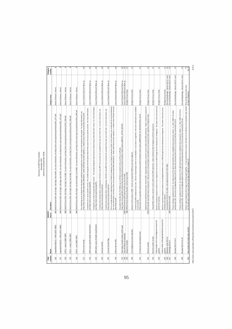
Dict

iona

ry o

f SEE

R*St

at V

aria

bles

N

ovem

ber 2

017

Sub

mis

sion

(rel

ease

d Ap

ril 2

018)

http

s://

seer

.can

cer.g

ov/d

ata-

soft

war

e/do

cum

enta

tion/

seer

stat

/nov

2017

/8

of 1

1

Fiel

d nu

mbe

rN

ame

NAA

CCR

Item

#D

escr

iptio

nCa

tego

ry n

ame

Cate

gory

nu

mbe

r

126

Expa

nded

EO

D(12

) - C

P64

(197

3-19

82)

840

NAA

CCR

Nam

e=EO

D--O

ld 1

3 Di

git-

-12t

h Di

git,

Item

#=8

40.

For m

ore

info

rmat

ion,

see

http

s://

seer

.can

cer.g

ov/m

anua

ls/hi

stor

ic/E

OD_

1977

.pdf

.Ex

tent

of D

iseas

e - H

istor

ic9

127

Expa

nded

EO

D(13

) - C

P65

(197

3-19

82)

840

NAA

CCR

Nam

e=EO

D--O

ld 1

3 Di

git-

-13t

h Di

git,

Item

#=8

40.

For m

ore

info

rmat

ion,

see

http

s://

seer

.can

cer.g

ov/m

anua

ls/hi

stor

ic/E

OD_

1977

.pdf

.Ex

tent

of D

iseas

e - H

istor

ic9

128

EOD

4 - e

xten

t (19

83-1

987)

860

NAA

CCR

Nam

e=EO

D--O

ld 4

Dig

it--3

rd D

igit,

Item

#=8

60.

For m

ore

info

rmat

ion,

see

http

s://

seer

.can

cer.g

ov/m

anua

ls/hi

stor

ic/E

OD_

1984

.pdf

.Ex

tent

of D

iseas

e - H

istor

ic9

129

EOD

4 - n

odes

(198

3-19

87)

860

NAA

CCR

Nam

e=EO

D--O

ld 4

Dig

it--4

th D

igit,

Item

#=8

60.

For m

ore

info

rmat

ion,

see

http

s://

seer

.can

cer.g

ov/m

anua

ls/hi

stor

ic/E

OD_

1984

.pdf

.Ex

tent

of D

iseas

e - H

istor

ic9

130

EOD

4 - s

ize

(198

3-19

87)

860

NAA

CCR

Nam

e=EO

D--O

ld 4

Dig

it--1

st a

nd 2

nd D

igit,

Item

#=8

60.

For m

ore

info

rmat

ion,

see

http

s://

seer

.can

cer.g

ov/m

anua

ls/hi

stor

ic/E

OD_

1984

.pdf

.Ex

tent

of D

iseas

e - H

istor

ic9

131

COD

to si

te re

code

Th

e un

derly

ing

caus

e of

dea

th fr

om th

e de

ath

cert

ifica

te w

as g

roup

ed in

to a

reco

de si

mila

r to

the

inci

denc

e sit

e re

code

. Fo

r mor

e in

form

atio

n, se

e ht

tps:

//se

er.c

ance

r.gov

/cod

reco

de/1

969_

d041

6201

2. S

tudy

cut

off d

ate

has b

een

appl

ied,

i.e.

cod

ed a

s aliv

e if

deat

h oc

curr

ed a

fter

stud

y cu

toff.

Caus

e of

Dea

th (C

OD)

and

Fol

low

-up

10

132

SEER

cau

se-s

peci

fic d

eath

cla

ssifi

catio

n

Crea

ted

for u

se in

cau

se-s

peci

fic su

rviv

al.

This

varia

ble

desig

nate

s tha

t the

per

son

died

of t

heir

canc

er fo

r cau

se-s

peci

fic su

rviv

al.

For m

ore

info

rmat

ion,

se

e ht

tps:

//se

er.c

ance

r.gov

/cau

sesp

ecifi

c.Ca

use

of D

eath

(CO

D) a

nd F

ollo

w-u

p10

133

SEER

oth

er c

ause

of d

eath

cla

ssifi

catio

n

Crea

ted

for u

se in

left

-tru

ncat

ed li

fe ta

ble

sess

ion.

Th

is va

riabl

e de

signa

tes t

hat t

he p

erso

n di

ed o

f cau

ses o

ther

than

thei

r can

cer.

For

mor

e in

form

atio

n,

see

http

s://

seer

.can

cer.g

ov/c

ause

spec

ific.

Caus

e of

Dea

th (C

OD)

and

Fol

low

-up

10

134

Surv

ival

mon

ths

Crea

ted

usin

g co

mpl

ete

date

s, in

clud

ing

days

, the

refo

re m

ay d

iffer

from

surv

ival

tim

e ca

lcul

ated

from

yea

r and

mon

th o

nly.

For

mor

e in

form

atio

n, se

e ht

tps:

//se

er.c

ance

r.gov

/sur

viva

ltim

e/.

Caus

e of

Dea

th (C

OD)

and

Fol

low

-up

10

135

Surv

ival

mon

ths f

lag

Crea

ted

usin

g co

mpl

ete

date

s, in

clud

ing

days

, the

refo

re m

ay d

iffer

from

surv

ival

tim

e ca

lcul

ated

from

yea

r and

mon

th o

nly.

For

mor

e in

form

atio

n, se

e ht

tps:

//se

er.c

ance

r.gov

/sur

viva

ltim

e/.

Caus

e of

Dea

th (C

OD)

and

Fol

low

-up

10

136

COD

to si

te re

c KM

This

is a

reco

de b

ased

on

unde

rlyin

g ca

use

of d

eath

to d

esig

nate

cau

se o

f dea

th in

to g

roup

s sim

ilar t

o th

e in

cide

nce

site

reco

de w

ith K

S an

d m

esot

helio

ma.

Fo

r mor

e in

form

atio

n, se

e ht

tps:

//se

er.c

ance

r.gov

/cod

reco

de/1

969_

d041

6201

2/.

Stud

y cu

toff

date

has

bee

n ap

plie

d, i.

e. c

oded

as a

live

if de

ath

occu

rred

af

ter s

tudy

cut

off.

Caus

e of

Dea

th (C

OD)

and

Fol

low

-up

10

137

Vita

l sta

tus r

ecod

e (s

tudy

cut

off u

sed)

An

y pa

tient

that

die

s aft

er th

e fo

llow

-up

cut-

off d

ate

is re

code

d to

aliv

e as

of t

he c

ut-o

ff da

te.

http

s://

seer

.can

cer.g

ov/d

ata-

soft

war

e/do

cum

enta

tion/

seer

stat

/nov

2017

/Tex

tDat

a.Fi

leDe

scrip

tion.

pdf#

VITA

L_ST

ATU

S_RE

CODE

Caus

e of

Dea

th (C

OD)

and

Fol

low

-up

1013

8Ty

pe o

f fol

low

-up

expe

cted

2180

NAA

CCR

Nam

e=SE

ER T

ype

of F

ollo

w-U

p, It

em #

=218

0Ca

use

of D

eath

(CO

D) a

nd F

ollo

w-u

p10

139

Sequ

ence

num

ber

380

NAA

CCR

Nam

e=Se

quen

ce N

umbe

r--C

entr

al, I

tem

#=3

80M

ultip

le P

rimar

y Fi

elds

11

140

Firs

t mal

igna

nt p

rimar

y in

dica

tor

Ba

sed

on a

ll th

e tu

mor

s in

SEER

. Tu

mor

s not

repo

rted

to S

EER

are

assu

med

mal

igna

nt.

Mul

tiple

Prim

ary

Fiel

ds11

141

Prim

ary

by in

tern

atio

nal r

ules

Crea

ted

usin

g IA

RC m

ultip

le p

rimar

y ru

les.

Did

not

incl

ude

beni

gn tu

mor

s or n

on-b

ladd

er in

situ

tum

ors i

n al

gorit

hm.

No

tum

or in

form

atio

n w

as m

odifi

ed

on a

ny re

cord

s.

http

s://

seer

.can

cer.g

ov/d

ata-

soft

war

e/do

cum

enta

tion/

seer

stat

/nov

2017

/Tex

tDat

a.Fi

leDe

scrip

tion.

pdf#

PRIM

ARY_

BY_I

NTE

RNAT

ION

AL_R

ULE

SM

ultip

le P

rimar

y Fi

elds

11

142

Reco

rd n

umbe

r21

90N

AACC

R N

ame=

SEER

Rec

ord

Num

ber,

Item

#=2

190.

Seq

uent

ially

num

bers

a p

erso

n's t

umor

s with

in e

ach

SEER

subm

issio

n. O

rder

is b

ased

on

sequ

ence

#.

All f

eder

ally

repo

rtab

le tu

mor

s (se

quen

ce #

< 6

0) a

re p

rior t

o al

l sta

te/r

egist

ry re

port

able

tum

ors (

sequ

ence

# 6

0+) r

egar

dles

s of d

iagn

osis

date

.M

ultip

le P

rimar

y Fi

elds

11

143

Reco

rd n

umbe

r rec

ode

S

eque

ntia

lly n

umbe

rs a

per

son'

s tum

ors w

ithin

eac

h SE

ER su

bmiss

ion.

Ord

er is

bas

ed o

n da

te o

f dia

gnos

is an

d th

en se

quen

ce #

. M

ultip

le P

rimar

y Fi

elds

11

144

Tota

l num

ber o

f in

situ

/mal

igna

nt tu

mor

s for

pa

tient

Ba

sed

on m

axim

um se

quen

ce n

umbe

r of a

ny m

alig

nant

/in si

tu tu

mor

s in

SEER

thro

ugh

the

last

rele

ased

yea

r of d

iagn

osis.

Thi

s val

ue is

the

sam

e ac

ross

all

tum

ors f

or a

per

son.

Mul

tiple

Prim

ary

Fiel

ds11

145

Tota

l num

ber o

f ben

ign/

bord

erlin

e tu

mor

s for

pa

tient

Ba

sed

on m

axim

um se

quen

ce n

umbe

r of a

ny b

enig

n/bo

rder

line

tum

ors i

n SE

ER th

roug

h th

e la

st re

leas

ed y

ear o

f dia

gnos

is. T

his v

alue

is th

e sa

me

acro

ss

all t

umor

s for

a p

erso

n.M

ultip

le P

rimar

y Fi

elds

1114

6Be

havi

or c

ode

ICD-

O-2

Co

nver

ted

from

ICD-

O-3

for 2

001+

and

cod

ed d

irect

ly fo

r 197

3-20

00.

Site

and

Mor

phol

ogy

- Hist

oric

(ICD

-O-1

and

I12

147

Hist

olog

y IC

D-O

-242

0N

AACC

R Ite

m #

=420

Site

and

Mor

phol

ogy

- Hist

oric

(ICD

-O-1

and

I12

148

Reco

de IC

D-O

-2 to

9

Prim

ary

site/

type

reco

ded

into

ICD-

9. A

n un

ders

core

in th

e rig

ht-m

ost p

ositi

on o

f an

unla

bele

d va

lue

repr

esen

ts a

bla

nk.

i.e.,

C00_

-C00

9 is

all v

alue

s st

artin

g w

ith C

00.

All t

umor

s not

orig

inal

ly c

oded

in IC

D-O

-2 w

ere

first

con

vert

ed fr

om IC

D-O

-1 o

r ICD

-O-3

and

then

con

vert

ed to

ICD-

9.Si

te a

nd M

orph

olog

y - H

istor

ic (I

CD-O

-1 a

nd I

12

149

Reco

de IC

D-O

-2 to

10

Pr

imar

y sit

e/ty

pe re

code

d in

to IC

D-10

. An

und

ersc

ore

in th

e rig

ht-m

ost p

ositi

on o

f an

unla

bele

d va

lue

repr

esen

ts a

bla

nk.

i.e.,

C00_

-C00

9 is

all v

alue

s st

artin

g w

ith C

00.

All t

umor

s not

orig

inal

ly c

oded

in IC

D-O

-2 w

ere

first

con

vert

ed fr

om IC

D-O

-1 o

r ICD

-O-3

and

then

con

vert

ed to

ICD-

10.

Site

and

Mor

phol

ogy

- Hist

oric

(ICD

-O-1

and

I12

150

Age

reco

de w

ith si

ngle

age

s and

85+

Pa

tient

's ag

e at

dia

gnos

is w

ith a

ll ag

es o

ver 8

5 gr

oupe

d to

geth

er.

In ra

te a

nd p

reva

lenc

e se

ssio

ns, t

his f

ield

can

be

sele

cted

as t

he p

opul

atio

n ag

e va

riabl

e (o

n th

e da

ta ta

b), i

n w

hich

cas

e it

will

be

in th

e Ag

e at

Dia

gnos

is ca

tego

ry (1

)Ra

ce a

nd A

ge (c

ase

data

onl

y)(o

r Age

at D

iagn

osis)

13(o

r 1)

95

Dict

iona

ry o

f SEE

R*St

at V

aria

bles

N

ovem

ber 2

017

Sub

mis

sion

(rel

ease

d Ap

ril 2

018)

http

s://

seer

.can

cer.g

ov/d

ata-

soft

war

e/do

cum

enta

tion/

seer

stat

/nov

2017

/9

of 1

1

Fiel

d nu

mbe

rN

ame

NAA

CCR

Item

#D

escr

iptio

nCa

tego

ry n

ame

Cate

gory

nu

mbe

r

151

Race

reco

de (W

, B, A

I, AP

I)

Caut

ion

shou

ld b

e ex

erci

sed

whe

n us

ing

this

varia

ble.

For

mor

e in

form

atio

n, se

e ht

tps:

//se

er.c

ance

r.gov

/see

rsta

t/va

riabl

es/s

eer/

race

_eth

nici

ty/.

Race

and

Age

(cas

e da

ta o

nly)

13

152

Orig

in re

code

NHI

A (H

ispa

nic,

Non

-His

p)

Caut

ion

shou

ld b

e ex

erci

sed

whe

n us

ing

this

varia

ble.

For

mor

e in

form

atio

n, se

e ht

tps:

//se

er.c

ance

r.gov

/see

rsta

t/va

riabl

es/s

eer/

race

_eth

nici

ty/.

Race

and

Age

(cas

e da

ta o

nly)

13

153

Race

and

orig

in re

code

(NHW

, NHB

, NHA

IAN

, N

HAPI

, His

pani

c)

Caut

ion

shou

ld b

e ex

erci

sed

whe

n us

ing

this

varia

ble.

For

mor

e in

form

atio

n, se

e ht

tps:

//se

er.c

ance

r.gov

/see

rsta

t/va

riabl

es/s

eer/

race

_eth

nici

ty/.

Race

and

Age

(cas

e da

ta o

nly)

13

154

Age

at d

iagn

osis

230

Age

at D

iagn

osis

is th

e pa

tient

's ag

e at

dia

gnos

is of

this

canc

er a

nd is

a th

ree

digi

t fie

ld b

ased

on

singl

e ye

ar o

f age

. Thi

s can

not

be

used

in a

rate

or

prev

alen

ce se

ssio

n to

link

to p

opul

atio

ns. S

ee A

SCII

text

file

des

crip

tion:

ht

tps:

//se

er.c

ance

r.gov

/dat

a-so

ftw

are/

docu

men

tatio

n/se

erst

at/n

ov20

17/T

extD

ata.

File

Desc

riptio

n.pd

f#AG

E_AT

_DIA

GN

OSI

S.Ra

ce a

nd A

ge (c

ase

data

onl

y)13

155

Race

/eth

nici

ty

Reco

de w

hich

giv

es p

riorit

y to

non

-whi

te ra

ces f

or p

erso

ns o

f mix

ed ra

ces.

Not

e th

at n

ot a

ll co

des w

ere

in e

ffect

for a

ll ye

ars.

For

mor

e in

form

atio

n, se

e ht

tps:

//se

er.c

ance

r.gov

/see

rsta

t/va

riabl

es/s

eer/

race

_eth

nici

ty/.

Race

and

Age

(cas

e da

ta o

nly)

13

156

NHI

A De

rived

His

p O

rigin

191

NAA

CCR

Item

#=1

91.

For m

ore

info

rmat

ion,

see

http

s://

seer

.can

cer.g

ov/s

eers

tat/

varia

bles

/see

r/ra

ce_e

thni

city

/.Ra

ce a

nd A

ge (c

ase

data

onl

y)13

157

IHS

Link

192

Inci

denc

e fil

es a

re p

erio

dica

lly li

nked

with

Indi

an H

ealth

Ser

vice

(IHS

) file

s to

iden

tify

Nat

ive

Amer

ican

s. T

he ra

ce re

code

use

s inf

orm

atio

n fr

om th

is fie

ld

and

race

to d

eter

min

e if

a pe

rson

is N

ativ

e Am

eric

an o

r not

. Se

e ht

tps:

//se

er.c

ance

r.gov

/see

rsta

t/va

riabl

es/s

eer/

race

_eth

nici

ty/

Race

and

Age

(cas

e da

ta o

nly)

13

158

Year

of b

irth

240

NAA

CCR

Nam

e=Bi

rth

Date

--Yea

r, Ite

m #

=240

. Th

e SE

ER d

ates

on

this

file

do n

ot h

ave

the

corr

espo

ndin

g da

te fl

ag fi

eld

incl

uded

. Bla

nk m

eans

unk

now

n.Da

tes

15

159

Mon

th o

f dia

gnos

is39

0N

AACC

R N

ame=

Date

of D

iagn

osis-

-Mon

th, I

tem

#=3

90. S

EER

date

s on

this

file

do n

ot h

ave

the

corr

espo

ndin

g da

te fl

ag fi

eld

incl

uded

. Bl

ank

mea

ns

unkn

own.

Date

s15

160

Mon

th o

f dia

gnos

is re

code

Es

timat

es m

onth

of d

iagn

osis,

bas

ed o

n ot

her k

now

n da

tes f

or th

at p

atie

nt, w

hen

actu

al m

onth

of d

iagn

osis

is un

know

n.

Date

s15

161

SS se

q #

- mal

+ins

(mos

t det

ail)

Si

te sp

ecifi

c se

quen

ce n

umbe

r of t

he tu

mor

ass

ocia

ted

with

the

site

clas

sific

atio

n sc

hem

e in

the

varia

ble

Site

- m

al+i

ns (m

ost d

etai

l). B

ased

on

all t

he

tum

ors i

n SE

ER.

Site

Spe

cific

Seq

uenc

e N

umbe

rs18

162

SS se

q #

1975

+ - m

al+i

ns (m

ost d

etai

l)

Site

spec

ific

sequ

ence

num

ber o

f the

tum

or a

ssoc

iate

d w

ith th

e sit

e cl

assif

icat

ion

sche

me

in th

e va

riabl

e Si

te -

mal

+ins

(mos

t det

ail).

Bas

ed o

n tu

mor

s di

agno

sed

1975

+.Si

te S

peci

fic S

eque

nce

Num

bers

18

163

SS se

q #

1992

+ - m

al+i

ns (m

ost d

etai

l)

Site

spec

ific

sequ

ence

num

ber o

f the

tum

or a

ssoc

iate

d w

ith th

e sit

e cl

assif

icat

ion

sche

me

in th

e va

riabl

e Si

te -

mal

+ins

(mos

t det

ail).

Bas

ed o

n tu

mor

s di

agno

sed

1992

+.Si

te S

peci

fic S

eque

nce

Num

bers

18

164

SS se

q #

2000

+ - m

al+i

ns (m

ost d

etai

l)

Site

spec

ific

sequ

ence

num

ber o

f the

tum

or a

ssoc

iate

d w

ith th

e sit

e cl

assif

icat

ion

sche

me

in th

e va

riabl

e Si

te -

mal

+ins

(mos

t det

ail).

Bas

ed o

n tu

mor

s di

agno

sed

2000

+.Si

te S

peci

fic S

eque

nce

Num

bers

18

165

Site

- m

al+i

ns (m

ost d

etai

l)

Shou

ld b

e us

ed in

con

junc

tion

with

and

onl

y w

ith th

e va

riabl

es S

S se

q #

- mal

+ins

(mos

t det

ail),

SS

seq

# 19

75+

- mal

+ins

(mos

t det

ail),

SS

seq

# 19

92+

- m

al+i

ns (m

ost d

etai

l), o

r SS

seq

# 20

00+

- mal

+ins

(mos

t det

ail).

Gro

upin

gs sh

ould

not

be

crea

ted.

Site

Spe

cific

Seq

uenc

e N

umbe

rs18

166

SS se

q #

- mal

(mos

t det

ail)

Si

te sp

ecifi

c se

quen

ce n

umbe

r of t

he tu

mor

ass

ocia

ted

with

the

site

clas

sific

atio

n sc

hem

e in

the

varia

ble

Site

- m

alig

nant

(mos

t det

ail).

Bas

ed o

n al

l the

tu

mor

s in

SEER

.Si

te S

peci

fic S

eque

nce

Num

bers

18

167

SS se

q #

1975

+ - m

al (m

ost d

etai

l)

Site

spec

ific

sequ

ence

num

ber o

f the

tum

or a

ssoc

iate

d w

ith th

e sit

e cl

assif

icat

ion

sche

me

in th

e va

riabl

e Si

te -

mal

igna

nt (m

ost d

etai

l). B

ased

on

tum

ors

diag

nose

d 19

75+.

Site

Spe

cific

Seq

uenc

e N

umbe

rs18

168

SS se

q #

1992

+ - m

al (m

ost d

etai

l)

Site

spec

ific

sequ

ence

num

ber o

f the

tum

or a

ssoc

iate

d w

ith th

e sit

e cl

assif

icat

ion

sche

me

in th

e va

riabl

e Si

te -

mal

igna

nt (m

ost d

etai

l). B

ased

on

tum

ors

diag

nose

d 19

92+.

Site

Spe

cific

Seq

uenc

e N

umbe

rs18

169

SS se

q #

2000

+ - m

al (m

ost d

etai

l)

Site

spec

ific

sequ

ence

num

ber o

f the

tum

or a

ssoc

iate

d w

ith th

e sit

e cl

assif

icat

ion

sche

me

in th

e va

riabl

e Si

te -

mal

igna

nt (m

ost d

etai

l). B

ased

on

tum

ors

diag

nose

d 20

00+.

Site

Spe

cific

Seq

uenc

e N

umbe

rs18

170

Site

- m

alig

nant

(mos

t det

ail)

Sh

ould

be

used

in c

onju

nctio

n w

ith a

nd o

nly

with

the

varia

bles

SS

seq

# - m

al (m

ost d

etai

l), S

S se

q #

1975

+ - m

al (m

ost d

etai

l), S

S se

q #

1992

+ - m

al (m

ost

deta

il), o

r SS

seq

# 20

00+

- mal

(mos

t det

ail).

Gro

upin

gs sh

ould

not

be

crea

ted.

Site

Spe

cific

Seq

uenc

e N

umbe

rs18

171

SS se

q #

- mal

+ins

(mid

det

ail)

Si

te sp

ecifi

c se

quen

ce n

umbe

r of t

he tu

mor

ass

ocia

ted

with

the

site

clas

sific

atio

n sc

hem

e in

the

varia

ble

Site

- m

al+i

ns (m

id d

etai

l). B

ased

on

all t

he

tum

ors i

n SE

ER.

Site

Spe

cific

Seq

uenc

e N

umbe

rs18

96

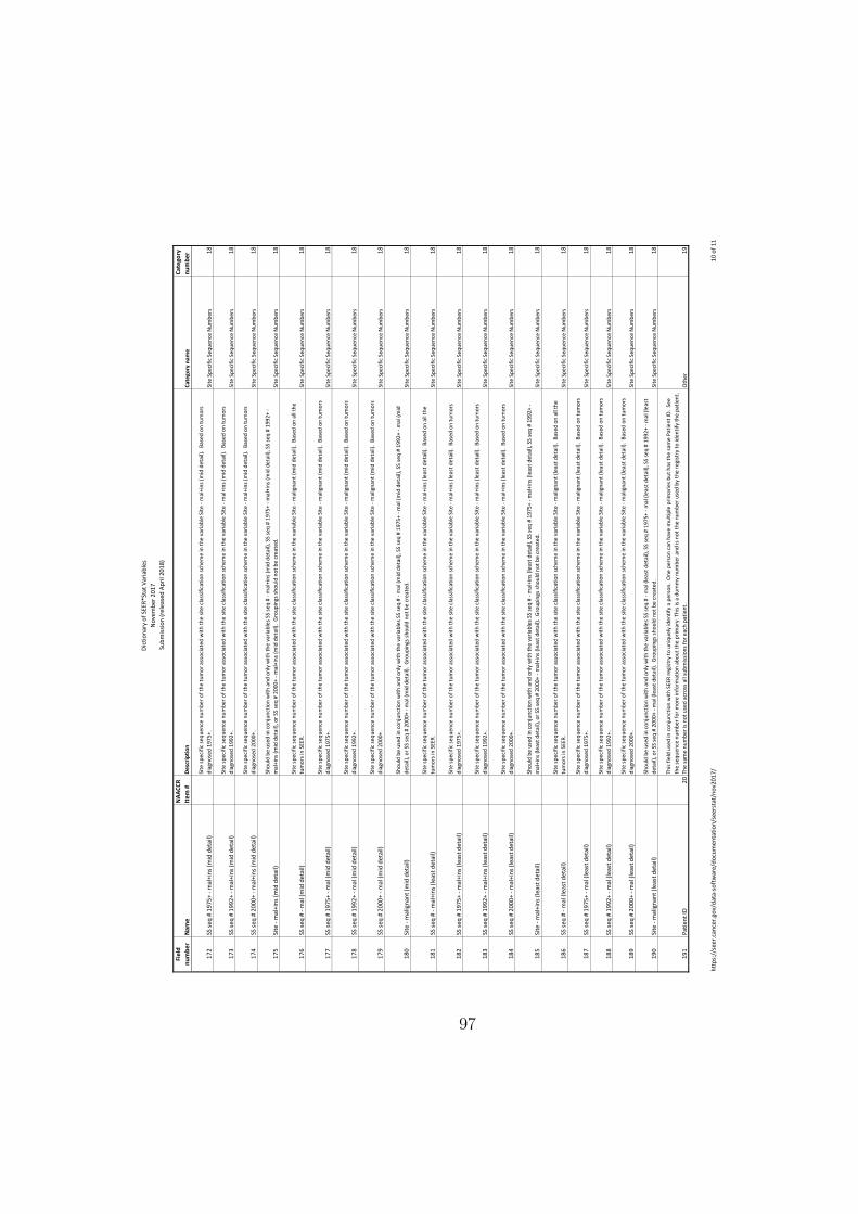
Dict

iona

ry o

f SEE

R*St

at V

aria

bles

N

ovem

ber 2

017

Sub

mis

sion

(rel

ease

d Ap

ril 2

018)

http

s://

seer

.can

cer.g

ov/d

ata-

soft

war

e/do

cum

enta

tion/

seer

stat

/nov

2017

/10

of 1

1

Fiel

d nu

mbe

rN

ame

NAA

CCR

Item

#D

escr

iptio

nCa

tego

ry n

ame

Cate

gory

nu

mbe

r

172

SS se

q #

1975

+ - m

al+i

ns (m

id d

etai

l)

Site

spec

ific

sequ

ence

num

ber o

f the

tum

or a

ssoc

iate

d w

ith th

e sit

e cl

assif

icat

ion

sche

me

in th

e va

riabl

e Si

te -

mal

+ins

(mid

det

ail).

Bas

ed o

n tu

mor

s di

agno

sed

1975

+.Si

te S

peci

fic S

eque

nce

Num

bers

18

173

SS se

q #

1992

+ - m

al+i

ns (m

id d

etai

l)

Site

spec

ific

sequ

ence

num

ber o

f the

tum

or a

ssoc

iate

d w

ith th

e sit

e cl

assif

icat

ion

sche

me

in th

e va

riabl

e Si

te -

mal

+ins

(mid

det

ail).

Bas

ed o

n tu

mor

s di

agno

sed

1992

+.Si

te S

peci

fic S

eque

nce

Num

bers

18

174

SS se

q #

2000

+ - m

al+i

ns (m

id d

etai

l)

Site

spec

ific

sequ

ence

num

ber o

f the

tum

or a

ssoc

iate

d w

ith th

e sit

e cl

assif

icat

ion

sche

me

in th

e va

riabl

e Si

te -

mal

+ins

(mid

det

ail).

Bas

ed o

n tu

mor

s di

agno

sed

2000

+.Si

te S

peci

fic S

eque

nce

Num

bers

18

175

Site

- m

al+i

ns (m

id d

etai

l)

Shou

ld b

e us

ed in

con

junc

tion

with

and

onl

y w

ith th

e va

riabl

es S

S se

q #

- mal

+ins

(mid

det

ail),

SS

seq

# 19

75+

- mal

+ins

(mid

det

ail),

SS

seq

# 19

92+

- m

al+i

ns (m

id d

etai

l), o

r SS

seq

# 20

00+

- mal

+ins

(mid

det

ail).

Gro

upin

gs sh

ould

not

be

crea

ted.

Site

Spe

cific

Seq

uenc

e N

umbe

rs18

176

SS se

q #

- mal

(mid

det

ail)

Si

te sp

ecifi

c se

quen

ce n

umbe

r of t

he tu

mor

ass

ocia

ted

with

the

site

clas

sific

atio

n sc

hem

e in

the

varia

ble

Site

- m

alig

nant

(mid

det

ail).

Bas

ed o

n al

l the

tu

mor

s in

SEER

.Si

te S

peci

fic S

eque

nce

Num

bers

18

177

SS se

q #

1975

+ - m

al (m

id d

etai

l)

Site

spec

ific

sequ

ence

num

ber o

f the

tum

or a

ssoc

iate

d w

ith th

e sit

e cl

assif

icat

ion

sche

me

in th

e va

riabl

e Si

te -

mal

igna

nt (m

id d

etai

l). B

ased

on

tum

ors

diag

nose

d 19

75+.

Site

Spe

cific

Seq

uenc

e N

umbe

rs18

178

SS se

q #

1992

+ - m

al (m

id d

etai

l)

Site

spec

ific

sequ

ence

num

ber o

f the

tum

or a

ssoc

iate

d w

ith th

e sit

e cl

assif

icat

ion

sche

me

in th

e va

riabl

e Si

te -

mal

igna

nt (m

id d

etai

l). B

ased

on

tum

ors

diag

nose

d 19

92+.

Site

Spe

cific

Seq

uenc

e N

umbe

rs18

179

SS se

q #

2000

+ - m

al (m

id d

etai

l)

Site

spec

ific

sequ

ence

num

ber o

f the

tum

or a

ssoc

iate

d w

ith th

e sit

e cl

assif

icat

ion

sche

me

in th

e va

riabl

e Si

te -

mal

igna

nt (m

id d

etai

l). B

ased

on

tum

ors

diag

nose

d 20

00+.

Site

Spe

cific

Seq

uenc

e N

umbe

rs18

180

Site

- m

alig

nant

(mid

det

ail)

Sh

ould

be

used

in c

onju

nctio

n w

ith a

nd o

nly

with

the

varia

bles

SS

seq

# - m

al (m

id d

etai

l), S

S se

q #

1975

+ - m

al (m

id d

etai

l), S

S se

q #

1992

+ - m

al (m

id

deta

il), o

r SS

seq

# 20

00+

- mal

(mid

det

ail).

Gro

upin

gs sh

ould

not

be

crea

ted.

Site

Spe

cific

Seq

uenc

e N

umbe

rs18

181

SS se

q #

- mal

+ins

(lea

st d

etai

l)

Site

spec

ific

sequ

ence

num

ber o

f the

tum

or a

ssoc

iate

d w

ith th

e sit

e cl

assif

icat

ion

sche

me

in th

e va

riabl

e Si

te -

mal

+ins

(lea

st d

etai

l). B

ased

on

all t

he

tum

ors i

n SE

ER.

Site

Spe

cific

Seq

uenc

e N

umbe

rs18

182

SS se

q #

1975

+ - m

al+i

ns (l

east

det

ail)

Si

te sp

ecifi

c se

quen

ce n

umbe

r of t

he tu

mor

ass

ocia

ted

with

the

site

clas

sific

atio

n sc

hem

e in

the

varia

ble

Site

- m

al+i

ns (l

east

det

ail).

Bas

ed o

n tu

mor

s di

agno

sed

1975

+.Si

te S

peci

fic S

eque

nce

Num

bers

18

183

SS se

q #

1992

+ - m

al+i

ns (l

east

det

ail)

Si

te sp

ecifi

c se

quen

ce n

umbe

r of t

he tu

mor

ass

ocia

ted

with

the

site

clas

sific

atio

n sc

hem

e in

the

varia

ble

Site

- m

al+i

ns (l

east

det

ail).

Bas

ed o

n tu

mor

s di

agno

sed

1992

+.Si

te S

peci

fic S

eque

nce

Num

bers

18

184

SS se

q #

2000

+ - m

al+i

ns (l

east

det

ail)

Si

te sp

ecifi

c se

quen

ce n

umbe

r of t

he tu

mor

ass

ocia

ted

with

the

site

clas

sific

atio

n sc

hem

e in

the

varia

ble

Site

- m

al+i

ns (l

east

det

ail).

Bas

ed o

n tu

mor

s di

agno

sed

2000

+.Si

te S

peci

fic S

eque

nce

Num

bers

18

185

Site

- m

al+i

ns (l

east

det

ail)

Sh

ould

be

used

in c

onju

nctio

n w

ith a

nd o

nly

with

the

varia

bles

SS

seq

# - m

al+i

ns (l

east

det

ail),

SS

seq

# 19

75+

- mal

+ins

(lea

st d

etai

l), S

S se

q #

1992

+ -

mal

+ins

(lea

st d

etai

l), o

r SS

seq

# 20

00+

- mal

+ins

(lea

st d

etai

l). G

roup

ings

shou

ld n

ot b

e cr

eate

d.Si

te S

peci

fic S

eque

nce

Num

bers

18

186

SS se

q #

- mal

(lea

st d

etai

l)

Site

spec

ific

sequ

ence

num

ber o

f the

tum

or a

ssoc

iate

d w

ith th

e sit

e cl

assif

icat

ion

sche

me

in th

e va

riabl

e Si

te -

mal

igna

nt (l

east

det

ail).

Bas

ed o

n al

l the

tu

mor

s in

SEER

.Si

te S

peci

fic S

eque

nce

Num

bers

18

187

SS se

q #

1975

+ - m

al (l

east

det

ail)

Si

te sp

ecifi

c se

quen

ce n

umbe

r of t

he tu

mor

ass

ocia

ted

with

the

site

clas

sific

atio

n sc

hem

e in

the

varia

ble

Site

- m

alig

nant

(lea

st d

etai

l). B

ased

on

tum

ors

diag

nose

d 19

75+.

Site

Spe

cific

Seq

uenc

e N

umbe

rs18

188

SS se

q #

1992

+ - m

al (l

east

det

ail)

Si

te sp

ecifi

c se

quen

ce n

umbe

r of t

he tu

mor

ass

ocia

ted

with

the

site

clas

sific

atio

n sc

hem

e in

the

varia

ble

Site

- m

alig

nant

(lea

st d

etai

l). B

ased

on

tum

ors

diag

nose

d 19

92+.

Site

Spe

cific

Seq

uenc

e N

umbe

rs18

189

SS se

q #

2000

+ - m

al (l

east

det

ail)

Si

te sp

ecifi

c se

quen

ce n

umbe

r of t

he tu

mor

ass

ocia

ted

with

the

site

clas

sific

atio

n sc

hem

e in

the

varia

ble

Site

- m

alig

nant

(lea

st d

etai

l). B

ased

on

tum

ors

diag

nose

d 20

00+.

Site

Spe

cific

Seq

uenc

e N

umbe

rs18

190

Site

- m

alig

nant

(lea

st d

etai

l)

Shou

ld b

e us

ed in

con

junc

tion

with

and

onl

y w

ith th

e va

riabl

es S

S se

q #

- mal

(lea

st d

etai

l), S

S se

q #

1975

+ - m

al (l

east

det

ail),

SS

seq

# 19

92+

- mal

(lea

st

deta

il), o

r SS

seq

# 20

00+

- mal

(lea

st d

etai

l). G

roup

ings

shou

ld n

ot b

e cr

eate

d.Si

te S

peci

fic S

eque

nce

Num

bers

18

191

Patie

nt ID

20

This

field

use

d in

con

junc

tion

with

SEE

R re

gist

ry to

uni

quel

y id

entif

y a

pers

on.

One

per

son

can

have

mul

tiple

prim

arie

s but

has

the

sam

e Pa

tient

ID.

See

the

sequ

ence

num

ber f

or m

ore

info

rmat

ion

abou

t the

prim

ary.

Thi

s is a

dum

my

num

ber a

nd is

not

the

num

ber u

sed

by th

e re

gist

ry to

iden

tify

the

patie

nt.

The

sam

e nu

mbe

r is n

ot u

sed

acro

ss a

ll su

bmiss

ions

for e

ach

patie

nt.

Oth

er19

97

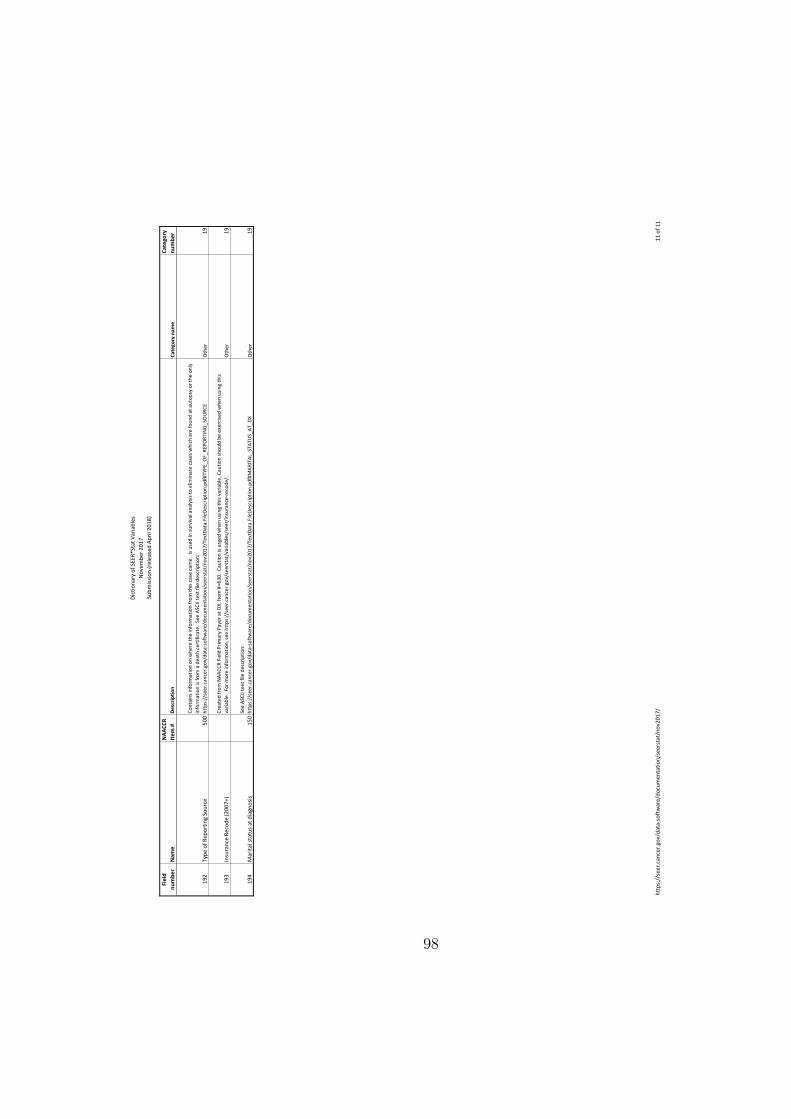
Dict

iona

ry o

f SEE

R*St

at V

aria

bles

N

ovem

ber 2

017

Sub

mis

sion

(rel

ease

d Ap

ril 2

018)

http

s://

seer

.can

cer.g

ov/d

ata-

soft

war

e/do

cum

enta

tion/

seer

stat

/nov

2017

/11

of 1

1

Fiel

d nu

mbe

rN

ame

NAA

CCR

Item

#D

escr

iptio

nCa

tego

ry n

ame

Cate

gory

nu

mbe

r

192

Type

of R

epor

ting

Sour

ce50

0

Cont

ains

info

rmat

ion

on w

here

the

info

rmat

ion

from

this

case

cam

e. I

s use

d in

surv

ival

ana

lysis

to e

limin

ate

case

s whi

ch a

re fo

und

at a

utop

sy o

r the

onl

y in

form

atio

n is

from

a d

eath

cer

tific

ate.

See

ASC

II te

xt fi

le d

escr

iptio

n:

http

s://

seer

.can

cer.g

ov/d

ata-

soft

war

e/do

cum

enta

tion/

seer

stat

/nov

2017

/Tex

tDat

a.Fi

leDe

scrip

tion.

pdf#

TYPE

_OF_

REPO

RTIN

G_S

OU

RCE

Oth

er19

193

Insu

ranc

e Re

code

(200

7+)

Crea

ted

from

NAA

CCR

Fiel

d Pr

imar

y Pa

yer a

t DX,

Item

#=6

30.

Caut

ion

is ur

ged

whe

n us

ing

this

varia

ble.

Cau

tion

shou

ld b

e ex

erci

sed

whe

n us

ing

this

varia

ble.

For

mor

e in

form

atio

n, se

e ht

tps:

//se

er.c

ance

r.gov

/see

rsta

t/va

riabl

es/s

eer/

insu

ranc

e-re

code

/.

Oth

er19

194

Mar

ital s

tatu

s at d

iagn

osis

150

See

ASCI

I tex

t file

des

crip

tion:

ht

tps:

//se

er.c

ance

r.gov

/dat

a-so

ftw

are/

docu

men

tatio

n/se

erst

at/n

ov20

17/T

extD

ata.

File

Desc

riptio

n.pd

f#M

ARIT

AL_S

TATU

S_AT

_DX

Oth

er19

98

Appendix B: An Example of Record in SEER Dataset

Here shows an example of one record of tumor (patient ID: 4552105) from the

specific database “Incidence - SEER 18 Regs Research Data + Hurricane Katrina

Impacted Louisiana Cases, Nov 2017 Sub (1973-2015 varying)”:

Feature Name ValueAge recode with <1 year olds 65-69 yearsRace recode (White, Black, Other) Other (American Indian/AK Native, Asian/Pacific Islander)Sex FemaleYear of diagnosis 2013SEER registry San Francisco-Oakland SMSA - 1973+Louisiana 2005 - 1st vs 2nd half of year Not applicable (1973-2004, 2005 not Louisiana, or 2006+)County 1State-county CA: Alameda County (06001)In research data YesCHSDA 2012 Not CHSDACHSDA Region Pacific CoastState CaliforniaSite recode ICD-O-3/WHO 2008 Lung and BronchusBehavior recode for analysis MalignantAYA site recode/WHO 2008 8.3 Carcinoma of trachea,bronchus, and lungLymphoma subtype recode/WHO 2008 UnclassifiedICCC site recode ICD-O-3/WHO 2008 XI(f) Other and unspecified carcinomasCS Schema v0204+ LungCS Schema - AJCC 6th Edition LungPrimary Site - labeled C34.1-Upper lobe, lungPrimary Site 341Histologic Type ICD-O-3 8140Behavior code ICD-O-3 MalignantGrade Moderately differentiated; Grade IILaterality Left - origin of primaryDiagnostic Confirmation Positive histologyICD-O-3 Hist/behav 8140/3: Adenocarcinoma, NOSICD-O-3 Hist/behav, malignant 8140/3: Adenocarcinoma, NOSHistology recode - broad groupings 8140-8389: adenomas and adenocarcinomasHistology recode - Brain groupings Not BrainICCC site rec extended ICD-O-3/WHO 2008 XI(f.4) Carcinomas of lungSite recode B ICD-O-3/WHO 2008 Lung and BronchusDerived AJCC Stage Group, 7th ed (2010+) IADerived AJCC Stage Group, 6th ed (2004+) IABreast - Adjusted AJCC 6th Stage (1988+) Blank(s)Derived AJCC - Flag (2004+) AJCC 6th ed derived from CS manual/coding instructions, v1.0AJCC stage 3rd edition (1988-2003) Blank(s)SEER modified AJCC stage 3rd (1988-2003) Blank(s)Lymphoma - Ann Arbor Stage (1983+) N/ADerived AJCC T, 7th ed (2010+) T1aDerived AJCC N, 7th ed (2010+) N0Derived AJCC M, 7th ed (2010+) M0Derived AJCC T, 6th ed (2004+) T1Derived AJCC N, 6th ed (2004+) N0Derived AJCC M, 6th ed (2004+) M0T value - based on AJCC 3rd (1988-2003) Blank(s)N value - based on AJCC 3rd (1988-2003) Blank(s)M value - based on AJCC 3rd (1988-2003) Blank(s)Breast - Adjusted AJCC 6th T (1988+) Blank(s)Breast - Adjusted AJCC 6th N (1988+) Blank(s)Breast - Adjusted AJCC 6th M (1988+) Blank(s)Derived SS1977 (2004+) LDerived SS2000 (2004+) LSummary stage 2000 (1998+) LocalizedSEER historic stage A LocalizedSEER summary stage 2000 (2001-2003) Blank(s)SEER summary stage 1977 (1995-2000) Blank(s)RX Summ–Surg Prim Site (1998+) 33RX Summ–Scope Reg LN Sur (2003+) 4 or more regional lymph nodes removedRX Summ–Surg Oth Reg/Dis (2003+) None; diagnosed at autopsyReason no cancer-directed surgery Surgery performedScope of reg lymph nd surg (1998-2002) Blank(s)RX Summ–Reg LN Examined (1998-2002) Blank(s)Surgery of oth reg/dis sites (1998-2002) Blank(s)CS tumor size (2004+) 20CS extension (2004+) 100CS lymph nodes (2004+) 0CS mets at dx (2004+) 0

99

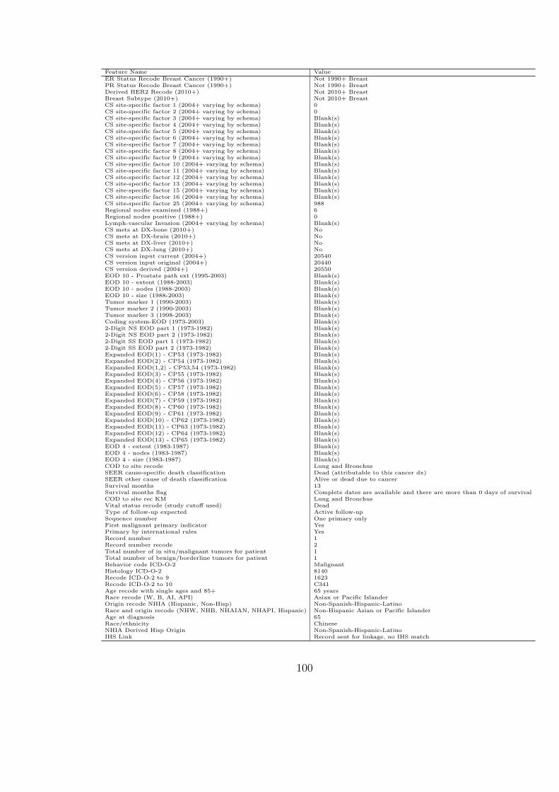
Feature Name ValueER Status Recode Breast Cancer (1990+) Not 1990+ BreastPR Status Recode Breast Cancer (1990+) Not 1990+ BreastDerived HER2 Recode (2010+) Not 2010+ BreastBreast Subtype (2010+) Not 2010+ BreastCS site-specific factor 1 (2004+ varying by schema) 0CS site-specific factor 2 (2004+ varying by schema) 0CS site-specific factor 3 (2004+ varying by schema) Blank(s)CS site-specific factor 4 (2004+ varying by schema) Blank(s)CS site-specific factor 5 (2004+ varying by schema) Blank(s)CS site-specific factor 6 (2004+ varying by schema) Blank(s)CS site-specific factor 7 (2004+ varying by schema) Blank(s)CS site-specific factor 8 (2004+ varying by schema) Blank(s)CS site-specific factor 9 (2004+ varying by schema) Blank(s)CS site-specific factor 10 (2004+ varying by schema) Blank(s)CS site-specific factor 11 (2004+ varying by schema) Blank(s)CS site-specific factor 12 (2004+ varying by schema) Blank(s)CS site-specific factor 13 (2004+ varying by schema) Blank(s)CS site-specific factor 15 (2004+ varying by schema) Blank(s)CS site-specific factor 16 (2004+ varying by schema) Blank(s)CS site-specific factor 25 (2004+ varying by schema) 988Regional nodes examined (1988+) 6Regional nodes positive (1988+) 0Lymph-vascular Invasion (2004+ varying by schema) Blank(s)CS mets at DX-bone (2010+) NoCS mets at DX-brain (2010+) NoCS mets at DX-liver (2010+) NoCS mets at DX-lung (2010+) NoCS version input current (2004+) 20540CS version input original (2004+) 20440CS version derived (2004+) 20550EOD 10 - Prostate path ext (1995-2003) Blank(s)EOD 10 - extent (1988-2003) Blank(s)EOD 10 - nodes (1988-2003) Blank(s)EOD 10 - size (1988-2003) Blank(s)Tumor marker 1 (1990-2003) Blank(s)Tumor marker 2 (1990-2003) Blank(s)Tumor marker 3 (1998-2003) Blank(s)Coding system-EOD (1973-2003) Blank(s)2-Digit NS EOD part 1 (1973-1982) Blank(s)2-Digit NS EOD part 2 (1973-1982) Blank(s)2-Digit SS EOD part 1 (1973-1982) Blank(s)2-Digit SS EOD part 2 (1973-1982) Blank(s)Expanded EOD(1) - CP53 (1973-1982) Blank(s)Expanded EOD(2) - CP54 (1973-1982) Blank(s)Expanded EOD(1,2) - CP53,54 (1973-1982) Blank(s)Expanded EOD(3) - CP55 (1973-1982) Blank(s)Expanded EOD(4) - CP56 (1973-1982) Blank(s)Expanded EOD(5) - CP57 (1973-1982) Blank(s)Expanded EOD(6) - CP58 (1973-1982) Blank(s)Expanded EOD(7) - CP59 (1973-1982) Blank(s)Expanded EOD(8) - CP60 (1973-1982) Blank(s)Expanded EOD(9) - CP61 (1973-1982) Blank(s)Expanded EOD(10) - CP62 (1973-1982) Blank(s)Expanded EOD(11) - CP63 (1973-1982) Blank(s)Expanded EOD(12) - CP64 (1973-1982) Blank(s)Expanded EOD(13) - CP65 (1973-1982) Blank(s)EOD 4 - extent (1983-1987) Blank(s)EOD 4 - nodes (1983-1987) Blank(s)EOD 4 - size (1983-1987) Blank(s)COD to site recode Lung and BronchusSEER cause-specific death classification Dead (attributable to this cancer dx)SEER other cause of death classification Alive or dead due to cancerSurvival months 13Survival months flag Complete dates are available and there are more than 0 days of survivalCOD to site rec KM Lung and BronchusVital status recode (study cutoff used) DeadType of follow-up expected Active follow-upSequence number One primary onlyFirst malignant primary indicator YesPrimary by international rules YesRecord number 1Record number recode 2Total number of in situ/malignant tumors for patient 1Total number of benign/borderline tumors for patient 1Behavior code ICD-O-2 MalignantHistology ICD-O-2 8140Recode ICD-O-2 to 9 1623Recode ICD-O-2 to 10 C341Age recode with single ages and 85+ 65 yearsRace recode (W, B, AI, API) Asian or Pacific IslanderOrigin recode NHIA (Hispanic, Non-Hisp) Non-Spanish-Hispanic-LatinoRace and origin recode (NHW, NHB, NHAIAN, NHAPI, Hispanic) Non-Hispanic Asian or Pacific IslanderAge at diagnosis 65Race/ethnicity ChineseNHIA Derived Hisp Origin Non-Spanish-Hispanic-LatinoIHS Link Record sent for linkage, no IHS match

100

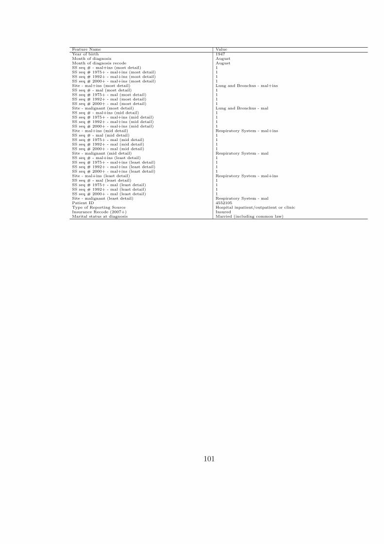
Feature Name ValueYear of birth 1947Month of diagnosis AugustMonth of diagnosis recode AugustSS seq # - mal+ins (most detail) 1SS seq # 1975+ - mal+ins (most detail) 1SS seq # 1992+ - mal+ins (most detail) 1SS seq # 2000+ - mal+ins (most detail) 1Site - mal+ins (most detail) Lung and Bronchus - mal+insSS seq # - mal (most detail) 1SS seq # 1975+ - mal (most detail) 1SS seq # 1992+ - mal (most detail) 1SS seq # 2000+ - mal (most detail) 1Site - malignant (most detail) Lung and Bronchus - malSS seq # - mal+ins (mid detail) 1SS seq # 1975+ - mal+ins (mid detail) 1SS seq # 1992+ - mal+ins (mid detail) 1SS seq # 2000+ - mal+ins (mid detail) 1Site - mal+ins (mid detail) Respiratory System - mal+insSS seq # - mal (mid detail) 1SS seq # 1975+ - mal (mid detail) 1SS seq # 1992+ - mal (mid detail) 1SS seq # 2000+ - mal (mid detail) 1Site - malignant (mid detail) Respiratory System - malSS seq # - mal+ins (least detail) 1SS seq # 1975+ - mal+ins (least detail) 1SS seq # 1992+ - mal+ins (least detail) 1SS seq # 2000+ - mal+ins (least detail) 1Site - mal+ins (least detail) Respiratory System - mal+insSS seq # - mal (least detail) 1SS seq # 1975+ - mal (least detail) 1SS seq # 1992+ - mal (least detail) 1SS seq # 2000+ - mal (least detail) 1Site - malignant (least detail) Respiratory System - malPatient ID 4552105Type of Reporting Source Hospital inpatient/outpatient or clinicInsurance Recode (2007+) InsuredMarital status at diagnosis Married (including common law)

101

Curriculum Vitae : Haoze Du

Personal Details

Gender: Male

Date of birth: May 20th, 1995

Place of birth: Xinxiang, China

Email: duhaoze1995@outlook.com

Research Interests

I am interested in machine learning and its application, and digital image process-

ing and recognition.

Education

09/2013–06/2017

Nanjing University of Aeronautics and Astronautics, ChinaBachelor of Engineering in Computer ScienceThesis: Research on Migrating xv6 OS to MIPS platform

Since 8/2017Wake Forest UniversityGraduate student in the Department of Computer Science

Working Experience

07/2016–01/2017Software Engineering InternPacteria, Wuxi

Since 8/2017Teaching AssistantWake Forest University

102

Scholarships

• Award of the Third Prize Outstanding Student Scholarship, Nanjing University

of Aeronautics and Astronautics (No.1321361) Nov.25, 2014.

• Award of the Third Prize Outstanding Student Scholarship, Nanjing University

of Aeronautics and Astronautics (No.1336388) Nov.20, 2015.

Papers

• Xianfang Wang, Haoze Du, Shuai Zhang. Dynamic multi-objective coopera-

tive optimization of biochemical process based on kinetic model and MOPSO.

Metallurgical and Mining Industry, 2015,7(6), pp:392-399.

• Xianfang Wang, Haoze Du, Jinglu Tan. Online Fault Diagnosis for Biochemi-

cal Process Based on FCM and SVM. Interdiscip Sci Comput Life Sci. Published

online 29 April 2016.

• WANG Xian-fang, WANG Sui-hua, DU Hao-ze, WANG Ping. Fault diagnosis

of chemical industry process based on FRS and SVM. Control and Decision,

2015,30(2), pp:353-356. (In Chinese)

Activities

• Member of UPE.

• Member of ACM and China Computer Federation.

103

• Award of Honorable Mention in the Mid-Atlantic Regional of ACM-ICPC. Nov,

2017

• Award of Honorable Mention in the 18th Annual MCM/ICM Competition.

USA. Apr 25, 2016.

• Award of the Second Prize of College Group A for C/C++C Program Design in

the 6th Annual Blue Bridge Cup National Software and Information Technology

Professional Talent Contest Jiangsu Division (No.010601451) Apr 17, 2015.

104