CS229 Lecture NotesTengyu Ma, Anand Avati, Kian Katanforoosh, and Andrew Ng

Deep LearningWe now begin our study of deep learning. In this set of notes, we give anoverview of neural networks, discuss vectorization and discuss training neuralnetworks with backpropagation.

1 Supervised Learning with Non-linear Mod-els

In the supervised learning setting (predicting y from the input x), supposeour model/hypothesis is hθ(x). In the past lectures, we have considered thecases when hθ(x) = θ⊤x (in linear regression or logistic regression) or hθ(x) =θ⊤ϕ(x) (where ϕ(x) is the feature map). A commonality of these two modelsis that they are linear in the parameters θ. Next we will consider learninggeneral family of models that are non-linear in both the parameters θand the inputs x. The most common non-linear models are neural networks,which we will define staring from the next section. For this section, it sufficesto think hθ(x) as an abstract non-linear model.1

Suppose {(x(i), y(i))}ni=1 are the training examples. For simplicity, we startwith the case where y(i) ∈ R and hθ(x) ∈ R.

Cost/loss function. We define the least square cost function for the i-thexample (x(i), y(i)) as

J (i)(θ) =1

2(hθ(x

(i))− y(i))2 (1.1)

1If a concrete example is helpful, perhaps think about the model hθ(x) = θ21x21 + θ22x

22 +

· · ·+ θ2dx2d in this subsection, even though it’s not a neural network.

1

2

and define the mean-square cost function for the dataset as

J(θ) =1

n

n∑i=1

J (i)(θ) (1.2)

which is same as in linear regression except that we introduce a constant1/n in front of the cost function to be consistent with the convention. Notethat multiplying the cost function with a scalar will not change the localminima or global minima of the cost function. Also note that the underlyingparameterization for hθ(x) is different from the case of linear regression,even though the form of the cost function is the same mean-squared loss.Throughout the notes, we use the words “loss” and “cost” interchangeably.

Optimizers (SGD). Commonly, people use gradient descent (GD), stochas-tic gradient (SGD), or their variants to optimize the loss function J(θ). GD’supdate rule can be written as2

θ := θ − α∇θJ(θ) (1.3)where α > 0 is often referred to as the learning rate or step size. Next, weintroduce a version of the SGD (Algorithm 1), which is lightly different fromthat in the first lecture notes.

Algorithm 1 Stochastic Gradient Descent1: Hyperparameter: learning rate α, number of total iteration niter.2: Initialize θ randomly.3: for i = 1 to niter do4: Sample j uniformly from {1, . . . , n}, and update θ by

θ := θ − α∇θJ(j)(θ) (1.4)

Oftentimes computing the gradient of B examples simultaneously for theparameter θ can be faster than computing B gradients separately due tohardware parallelization. Therefore, a mini-batch version of SGD is mostcommonly used in deep learning, as shown in Algorithm 2. There are alsoother variants of the SGD or mini-batch SGD with slightly different samplingschemes.2Recall that, as defined in the previous lecture notes, we use the notation “a := b” todenote an operation (in a computer program) in which we set the value of a variable ato be equal to the value of b. In other words, this operation overwrites a with the valueof b. In contrast, we will write “a = b” when we are asserting a statement of fact, thatthe value of a is equal to the value of b.

3

Algorithm 2 Mini-batch Stochastic Gradient Descent1: Hyperparameters: learning rate α, batch size B, # iterations niter.2: Initialize θ randomly3: for i = 1 to niter do4: Sample B examples j1, . . . , jB (without replacement) uniformly from

{1, . . . , n}, and update θ by

θ := θ − α

B

B∑k=1

∇θJ(jk)(θ) (1.5)

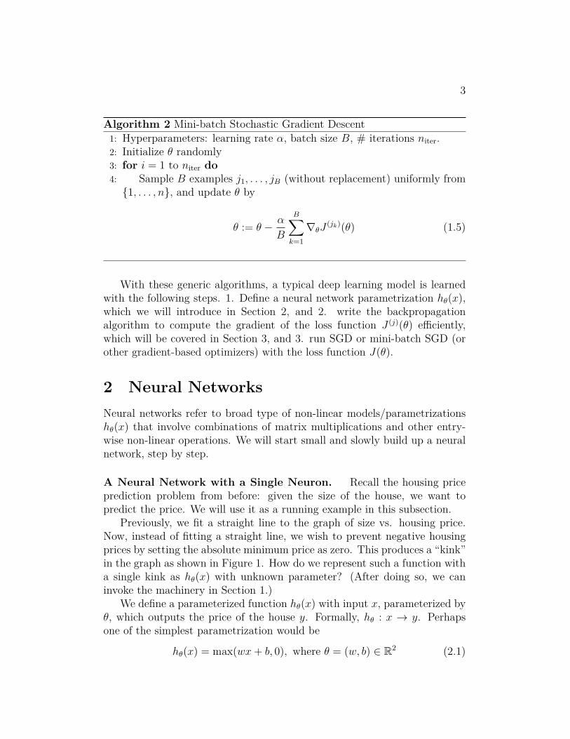
With these generic algorithms, a typical deep learning model is learnedwith the following steps. 1. Define a neural network parametrization hθ(x),which we will introduce in Section 2, and 2. write the backpropagationalgorithm to compute the gradient of the loss function J (j)(θ) efficiently,which will be covered in Section 3, and 3. run SGD or mini-batch SGD (orother gradient-based optimizers) with the loss function J(θ).

2 Neural NetworksNeural networks refer to broad type of non-linear models/parametrizationshθ(x) that involve combinations of matrix multiplications and other entry-wise non-linear operations. We will start small and slowly build up a neuralnetwork, step by step.

A Neural Network with a Single Neuron. Recall the housing priceprediction problem from before: given the size of the house, we want topredict the price. We will use it as a running example in this subsection.

Previously, we fit a straight line to the graph of size vs. housing price.Now, instead of fitting a straight line, we wish to prevent negative housingprices by setting the absolute minimum price as zero. This produces a “kink”in the graph as shown in Figure 1. How do we represent such a function witha single kink as hθ(x) with unknown parameter? (After doing so, we caninvoke the machinery in Section 1.)

We define a parameterized function hθ(x) with input x, parameterized byθ, which outputs the price of the house y. Formally, hθ : x → y. Perhapsone of the simplest parametrization would be

hθ(x) = max(wx+ b, 0), where θ = (w, b) ∈ R2 (2.1)

4

Here hθ(x) returns a single value: (wx+b) or zero, whichever is greater. Inthe context of neural networks, the function max{t, 0} is called a ReLU (pro-nounced “ray-lu”), or rectified linear unit, and often denoted by ReLU(t) ≜max{t, 0}.

Generally, a one-dimensional non-linear function that maps R to R such asReLU is often referred to as an activation function. The model hθ(x) is saidto have a single neuron partly because it has a single non-linear activationfunction. (We will discuss more about why a non-linear activation is calledneuron.)

When the input x ∈ Rd has multiple dimensions, a neural network witha single neuron can be written as

hθ(x) = ReLU(w⊤x+ b), where w ∈ Rd, b ∈ R, and θ = (w, b) (2.2)

The term b is often referred to as the “bias”, and the vector w is referredto as the weight vector. Such a neural network has 1 layer. (We will definewhat multiple layers mean in the sequel.)

Stacking Neurons. A more complex neural network may take the singleneuron described above and “stack” them together such that one neuronpasses its output as input into the next neuron, resulting in a more complexfunction.

Let us now deepen the housing prediction example. In addition to the sizeof the house, suppose that you know the number of bedrooms, the zip codeand the wealth of the neighborhood. Building neural networks is analogousto Lego bricks: you take individual bricks and stack them together to buildcomplex structures. The same applies to neural networks: we take individualneurons and stack them together to create complex neural networks.

Given these features (size, number of bedrooms, zip code, and wealth),we might then decide that the price of the house depends on the maximumfamily size it can accommodate. Suppose the family size is a function of thesize of the house and number of bedrooms (see Figure 2). The zip code mayprovide additional information such as how walkable the neighborhood is(i.e., can you walk to the grocery store or do you need to drive everywhere).Combining the zip code with the wealth of the neighborhood may predictthe quality of the local elementary school. Given these three derived features(family size, walkable, school quality), we may conclude that the price of thehome ultimately depends on these three features.

Formally, the input to a neural network is a set of input featuresx1, x2, x3, x4. We denote the intermediate variables for “family size”, “walk-able”, and “school quality” by a1, a2, a3 (these ai’s are often referred to as

5

500 1000 1500 2000 2500 3000 3500 4000 4500 5000

0

100

200

300

400

500

600

700

800

900

1000

housing prices

square feet

pri

ce (

in $

10

00

)

Figure 1: Housing prices with a “kink” in the graph.

Family Size

School Quality

Walkable

Size

# Bedrooms

Zip Code

Wealth

Price

y

Figure 2: Diagram of a small neural network for predicting housing prices.

“hidden units” or “hidden neurons”). We represent each of the ai’s as a neu-ral network with a single neuron with a subset of x1, . . . , x4 as inputs. Thenas in Figure 1, we will have the parameterization:

a1 = ReLU(θ1x1 + θ2x2 + θ3)

a2 = ReLU(θ4x3 + θ5)

a3 = ReLU(θ6x3 + θ7x4 + θ8)

where (θ1, · · · , θ8) are parameters. Now we represent the final output hθ(x)as another linear function with a1, a2, a3 as inputs, and we get3

hθ(x) = θ9a1 + θ10a2 + θ11a3 + θ12 (2.3)3Typically, for multi-layer neural network, at the end, near the output, we don’t applyReLU, especially when the output is not necessarily a positive number.

6

where θ contains all the parameters (θ1, · · · , θ12).Now we represent the output as a quite complex function of x with pa-

rameters θ. Then you can use this parametrization hθ with the machinery ofSection 1 to learn the parameters θ.

Inspiration from Biological Neural Networks. As the name suggests,artificial neural networks were inspired by biological neural networks. Thehidden units a1, . . . , am correspond to the neurons in a biological neural net-work, and the parameters θi’s correspond to the synapses. However, it’sunclear how similar the modern deep artificial neural networks are to the bi-ological ones. For example, perhaps not many neuroscientists think biologicalneural networks could have 1000 layers, while some modern artificial neuralnetworks do (we will elaborate more on the notion of layers.) Moreover, it’san open question whether human brains update their neural networks in away similar to the way that computer scientists learn artificial neural net-works (using backpropagation, which we will introduce in the next section.).

Two-layer Fully-Connected Neural Networks. We constructed theneural network in equation (2.3) using a significant amount of prior knowl-edge/belief about how the “family size”, “walkable”, and “school quality” aredetermined by the inputs. We implicitly assumed that we know the familysize is an important quantity to look at and that it can be determined by onlythe “size” and “# bedrooms”. Such a prior knowledge might not be availablefor other applications. It would be more flexible and general to have a genericparameterization. A simple way would be to write the intermediate variablea1 as a function of all x1, . . . , x4:

a1 = ReLU(w⊤1 x+ b1), where w1 ∈ R4 and b1 ∈ R (2.4)

a2 = ReLU(w⊤2 x+ b2), where w2 ∈ R4 and b2 ∈ R

a3 = ReLU(w⊤3 x+ b3), where w3 ∈ R4 and b3 ∈ R

We still define hθ(x) using equation (2.3) with a1, a2, a3 being definedas above. Thus we have a so-called fully-connected neural network asvisualized in the dependency graph in Figure 2 because all the intermediatevariables ai’s depend on all the inputs xi’s.

For full generality, a two-layer fully-connected neural network with mhidden units and d dimensional input x ∈ Rd is defined as

∀j ∈ [1, ...,m], zj = w[1]j

⊤x+ b

[1]j where w

[1]j ∈ Rd, b

[1]j ∈ R (2.5)

7

Figure 3: Diagram of a two-layer fully connected neural network. Each edgefrom node xi to node aj indicates that aj depends on xi. The edge from xi

to aj is associated with the weight (w[1]j )i which denotes the i-th coordinate

of the vector w[1]j . The activation aj can be computed by taking the ReLUof

the weighted sum of xi’s with the weights being the weights associated withthe incoming edges, that is, aj = ReLU(

∑di=1(w

[1]j )ixi).

aj = ReLU(zj),

a = [a1, . . . , am]⊤ ∈ Rm

hθ(x) = w[2]⊤a+ b[2] where w[2] ∈ Rm, b[2] ∈ R, (2.6)

Note that by default the vectors in Rd are viewed as column vectors, andin particular a is a column vector with components a1, a2, ..., am. The indices[1] and [2] are used to distinguish two sets of parameters: the w

[1]j ’s (each of

which is a vector in Rd) and w[2] (which is a vector in Rm). We will havemore of these later.

Vectorization. Before we introduce neural networks with more layers andmore complex structures, we will simplify the expressions for neural networkswith more matrix and vector notations. Another important motivation ofvectorization is the speed perspective in the implementation. In order toimplement a neural network efficiently, one must be careful when using forloops. The most natural way to implement equation (2.5) in code is perhapsto use a for loop. In practice, the dimensionalities of the inputs and hiddenunits are high. As a result, code will run very slowly if you use for loops.

8

Leveraging the parallelism in GPUs is/was crucial for the progress of deeplearning.

This gave rise to vectorization. Instead of using for loops, vectorizationtakes advantage of matrix algebra and highly optimized numerical linearalgebra packages (e.g., BLAS) to make neural network computations runquickly. Before the deep learning era, a for loop may have been sufficienton smaller datasets, but modern deep networks and state-of-the-art datasetswill be infeasible to run with for loops.

We vectorize the two-layer fully-connected neural network as below. Wedefine a weight matrix W [1] in Rm×d as the concatenation of all the vectorsw

[1]j ’s in the following way:

W [1] =

— w

[1]1

⊤—

— w[1]2

⊤—

...— w

[1]m

⊤—

∈ Rm×d (2.7)

Now by the definition of matrix vector multiplication, we can write z =[z1, . . . , zm]

⊤ ∈ Rm asz1......zm

︸ ︷︷ ︸z ∈ Rm×1

=

— w

[1]1

⊤—

— w[1]2

⊤—

...— w

[1]m

⊤—

︸ ︷︷ ︸W [1] ∈ Rm×d

x1

x2...xd

︸ ︷︷ ︸x ∈ Rd×1

+

b[1]1

b[1]2...b[1]m

︸ ︷︷ ︸

b[1] ∈ Rm×1

(2.8)

Or succinctly,

z = W [1]x+ b[1] (2.9)

We remark again that a vector in Rd in this notes, following the conventionspreviously established, is automatically viewed as a column vector, and canalso be viewed as a d × 1 dimensional matrix. (Note that this is differentfrom numpy where a vector is viewed as a row vector in broadcasting.)

Computing the activations a ∈ Rm from z ∈ Rm involves an element-wise non-linear application of the ReLU function, which can be computed inparallel efficiently. Overloading ReLU for element-wise application of ReLU

9

(meaning, for a vector t ∈ Rd, ReLU(t) is a vector such that ReLU(t)i =ReLU(ti)), we have

a = ReLU(z) (2.10)

Define W [2] = [w[2]⊤] ∈ R1×m similarly. Then, the model in equation (2.6)can be summarized as

a = ReLU(W [1]x+ b[1])

hθ(x) = W [2]a+ b[2] (2.11)

Here θ consists of W [1],W [2] (often referred to as the weight matrices) andb[1], b[2] (referred to as the biases). The collection of W [1], b[1] is referred to asthe first layer, and W [2], b[2] the second layer. The activation a is referred to asthe hidden layer. A two-layer neural network is also called one-hidden-layerneural network.

Multi-layer fully-connected neural networks. With this succinct no-tations, we can stack more layers to get a deeper fully-connected neu-ral network. Let r be the number of layers (weight matrices). LetW [1], . . . ,W [r], b[1], . . . , b[r] be the weight matrices and biases of all the layers.Then a multi-layer neural network can be written as

a[1] = ReLU(W [1]x+ b[1])

a[2] = ReLU(W [2]a[1] + b[2])

· · ·a[r−1] = ReLU(W [r−1]a[r−2] + b[r−1])

hθ(x) = W [r]a[r−1] + b[r] (2.12)

We note that the weight matrices and biases need to have compatibledimensions for the equations above to make sense. If a[k] has dimension mk,then the weight matrix W [k] should be of dimension mk×mk−1, and the biasb[k] ∈ Rmk . Moreover, W [1] ∈ Rm1×d and W [r] ∈ R1×mr−1 .

The total number of neurons in the network is m1 + · · · + mr, and thetotal number of parameters in this network is (d+1)m1+(m1+1)m2+ · · ·+(mr−1 + 1)mr.

Sometimes for notational consistency we also write a[0] = x, and a[r] =hθ(x). Then we have simple recursion that

a[k] = ReLU(W [k]a[k−1] + b[k]),∀k = 1, . . . , r − 1 (2.13)

10

Note that this would have be true for k = r if there were an additionalReLU in equation (2.12), but often people like to make the last layer linear(aka without a ReLU) so that negative outputs are possible and it’s easierto interpret the last layer as a linear model. (More on the interpretability atthe “connection to kernel method” paragraph of this section.)

Other activation functions. The activation function ReLU can be re-placed by many other non-linear function σ(·) that maps R to R such as

σ(z) =1

1 + e−z(sigmoid) (2.14)

σ(z) =ez − e−z

ez + e−z(tanh) (2.15)

Why do we not use the identity function for σ(z)? That is, whynot use σ(z) = z? Assume for sake of argument that b[1] and b[2] are zeros.Suppose σ(z) = z, then for two-layer neural network, we have that

hθ(x) = W [2]a[1] (2.16)= W [2]σ(z[1]) by definition (2.17)= W [2]z[1] since σ(z) = z (2.18)= W [2]W [1]x from Equation (2.8) (2.19)= W̃x where W̃ = W [2]W [1] (2.20)

Notice how W [2]W [1] collapsed into W̃ .This is because applying a linear function to another linear function will

result in a linear function over the original input (i.e., you can construct a W̃such that W̃x = W [2]W [1]x). This loses much of the representational powerof the neural network as often times the output we are trying to predicthas a non-linear relationship with the inputs. Without non-linear activationfunctions, the neural network will simply perform linear regression.

Connection to the Kernel Method. In the previous lectures, we coveredthe concept of feature maps. Recall that the main motivation for featuremaps is to represent functions that are non-linear in the input x by θ⊤ϕ(x),where θ are the parameters and ϕ(x), the feature map, is a handcraftedfunction non-linear in the raw input x. The performance of the learning

11

algorithms can significantly depends on the choice of the feature map ϕ(x).Oftentimes people use domain knowledge to design the feature map ϕ(x) thatsuits the particular applications. The process of choosing the feature mapsis often referred to as feature engineering.

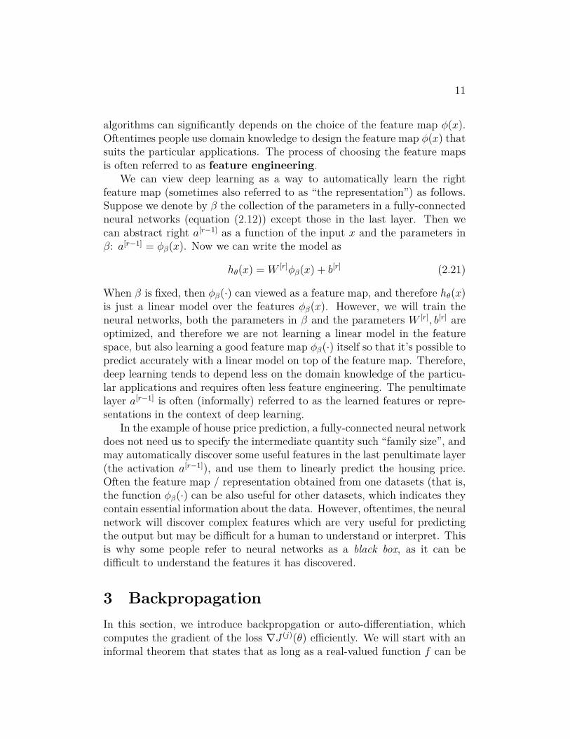
We can view deep learning as a way to automatically learn the rightfeature map (sometimes also referred to as “the representation”) as follows.Suppose we denote by β the collection of the parameters in a fully-connectedneural networks (equation (2.12)) except those in the last layer. Then wecan abstract right a[r−1] as a function of the input x and the parameters inβ: a[r−1] = ϕβ(x). Now we can write the model as

hθ(x) = W [r]ϕβ(x) + b[r] (2.21)

When β is fixed, then ϕβ(·) can viewed as a feature map, and therefore hθ(x)is just a linear model over the features ϕβ(x). However, we will train theneural networks, both the parameters in β and the parameters W [r], b[r] areoptimized, and therefore we are not learning a linear model in the featurespace, but also learning a good feature map ϕβ(·) itself so that it’s possible topredict accurately with a linear model on top of the feature map. Therefore,deep learning tends to depend less on the domain knowledge of the particu-lar applications and requires often less feature engineering. The penultimatelayer a[r−1] is often (informally) referred to as the learned features or repre-sentations in the context of deep learning.

In the example of house price prediction, a fully-connected neural networkdoes not need us to specify the intermediate quantity such “family size”, andmay automatically discover some useful features in the last penultimate layer(the activation a[r−1]), and use them to linearly predict the housing price.Often the feature map / representation obtained from one datasets (that is,the function ϕβ(·) can be also useful for other datasets, which indicates theycontain essential information about the data. However, oftentimes, the neuralnetwork will discover complex features which are very useful for predictingthe output but may be difficult for a human to understand or interpret. Thisis why some people refer to neural networks as a black box, as it can bedifficult to understand the features it has discovered.

3 BackpropagationIn this section, we introduce backpropgation or auto-differentiation, whichcomputes the gradient of the loss ∇J (j)(θ) efficiently. We will start with aninformal theorem that states that as long as a real-valued function f can be

12

efficiently computed/evaluated by a differentiable network or circuit, then itsgradient can be efficiently computed in a similar time. We will then showhow to do this concretely for fully-connected neural networks.

Because the formality of the general theorem is not the main focus here,we will introduce the terms with informal definitions. By a differentiablecircuit or a differentiable network, we mean a composition of a sequence ofdifferentiable arithmetic operations (additions, subtraction, multiplication,divisions, etc) and elementary differentiable functions (ReLU, exp, log, sin,cos, etc.). Let the size of the circuit be the total number of such operationsand elementary functions. We assume that each of the operations and func-tions, and their derivatives or partial derivatives can be computed in O(1)time in the computer.Theorem 3.1 : [backpropagation or auto-differentiation, informally stated]Suppose a differentiable circuit of size N computes a real-valued functionf : Rℓ → R. Then, the gradient ∇f can be computed in time O(N), by acircuit of size O(N).4

We note that the loss function J (j)(θ) for the j-th example can be indeedcomputed by a sequence of operations and functions involving additions,subtraction, multiplications, and non-linear activations. Thus the theoremsuggests that we should be able to compute ∇J (j)(θ) in a similar time to thatfor computing J (j)(θ) itself. This does not only apply to the fully-connectedneural network introduced in Section 2, but also many other types of neuralnetworks.

In the rest of the section, we will showcase how to compute the gradient ofthe loss efficiently for fully-connected neural networks using backpropagation.Even though auto-differentiation or backpropagation is implemented in allthe deep learning packages such as TensorFlow and PyTorch, understandingit is very helpful for gaining insights into the workings of deep learning.

3.1 Preliminary: chain ruleWe first recall the chain rule in calculus. Suppose the variable J depends onthe variables θ1, . . . , θp via the intermediate variables g1, . . . , gk:

gj = gj(θ1, . . . , θp),∀j ∈ {1, · · · , k} (3.1)4We note if the output of the function f does not depend on some of the input coordinates,then we set by default the gradient w.r.t that coordinate to zero. Setting to zero doesnot count towards the total runtime here in our accounting scheme. This is why whenN ≤ ℓ, we can compute the gradient in O(N) time, which might be potentially even lessthan ℓ.

13

J = J(g1, . . . , gk) (3.2)

Here we overload the meaning of gj’s: they denote both the intermediatevariables but also the functions used to compute the intermediate variables.Then, by the chain rule, we have that ∀i,

∂J

∂θi=

k∑j=1

∂J

∂gj

∂gj∂θi

(3.3)

For the ease of invoking the chain rule in the following subsections in variousways, we will call J the output variable, g1, . . . , gk intermediate variables,and θ1, . . . , θp the input variables in the chain rule.

3.2 Backpropagation for two-layer neural networksNow we consider the two-layer neural network defined in equation (2.11).Our general approach is to first unpack the vectorized notation to scalarform to apply the chain rule, but as soon as we finish the derivation, we willpack the scalar equations back to a vectorized form to keep the notationssuccinct.

Recall the following equations are used for the computation of the loss J :

z = W [1]x+ b[1]

a = ReLU(z)

hθ(x) ≜ o = W [2]a+ b[2]

J =1

2(y − o)2 (3.4)

Recall that W [1] ∈ Rm×d, W [2] ∈ R1×m, and b[1], z, a ∈ Rm, and o, y, b[2] ∈ R.Recall that a vector in Rd is automatically interpreted as a column vector(like a matrix in Rd×1) if need be.5

Computing ∂J∂W [2] . Suppose W [2] = [W

[2]1 , . . . ,W

[2]m ]. We start by comput-

ing ∂J

∂W[2]i

using the chain rule (3.3) with o as the intermediate variable.

∂J

∂W[2]i

=∂J

∂o· ∂o

∂W[2]i

5We also note that even though this is the convention in math, it’s different from theconvention in numpy where an one dimensional array will be automatically interpreted asa row vector.

14

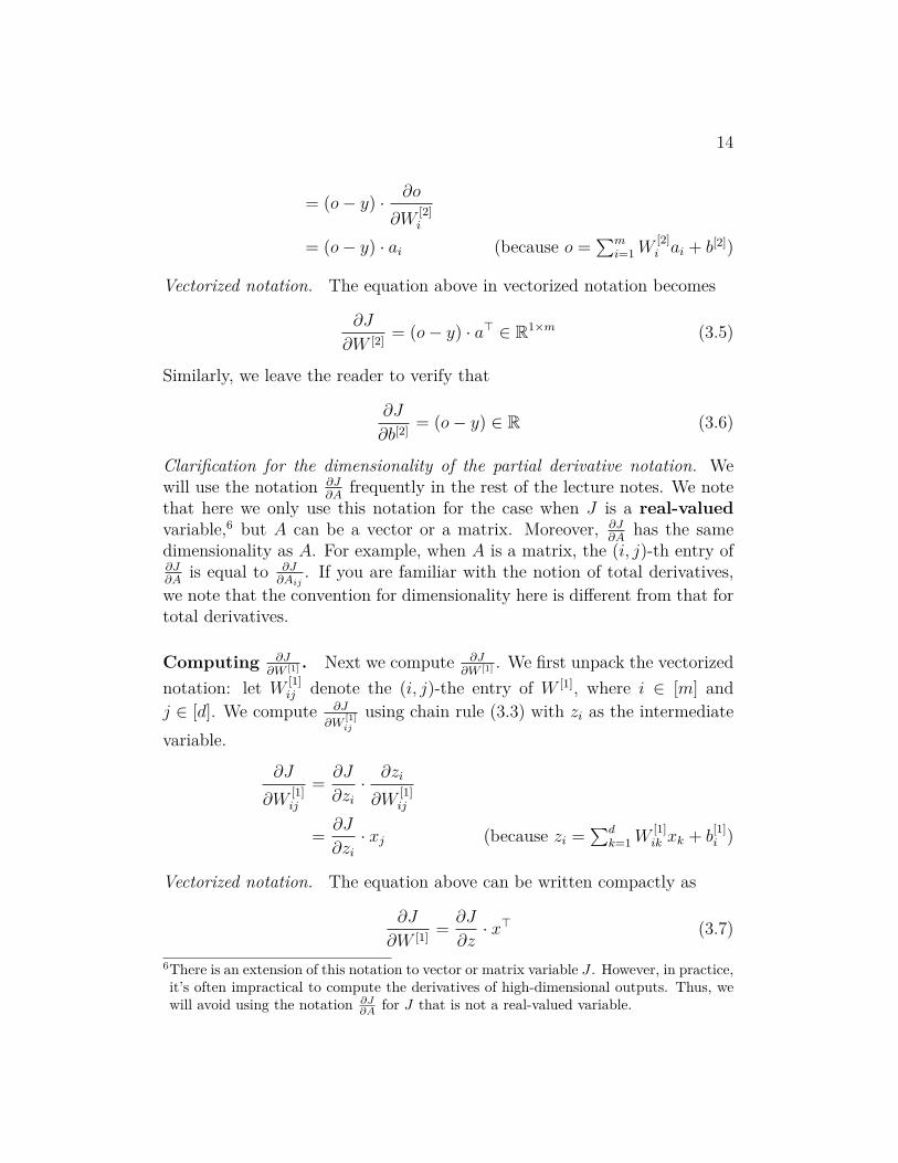
= (o− y) · ∂o

∂W[2]i

= (o− y) · ai (because o =∑m

i=1 W[2]i ai + b[2])

Vectorized notation. The equation above in vectorized notation becomes

∂J

∂W [2]= (o− y) · a⊤ ∈ R1×m (3.5)

Similarly, we leave the reader to verify that

∂J

∂b[2]= (o− y) ∈ R (3.6)

Clarification for the dimensionality of the partial derivative notation. Wewill use the notation ∂J

∂Afrequently in the rest of the lecture notes. We note

that here we only use this notation for the case when J is a real-valuedvariable,6 but A can be a vector or a matrix. Moreover, ∂J

∂Ahas the same

dimensionality as A. For example, when A is a matrix, the (i, j)-th entry of∂J∂A

is equal to ∂J∂Aij

. If you are familiar with the notion of total derivatives,we note that the convention for dimensionality here is different from that fortotal derivatives.

Computing ∂J∂W [1] . Next we compute ∂J

∂W [1] . We first unpack the vectorizednotation: let W

[1]ij denote the (i, j)-the entry of W [1], where i ∈ [m] and

j ∈ [d]. We compute ∂J

∂W[1]ij

using chain rule (3.3) with zi as the intermediatevariable.

∂J

∂W[1]ij

=∂J

∂zi· ∂zi

∂W[1]ij

=∂J

∂zi· xj (because zi =

∑dk=1W

[1]ik xk + b

[1]i )

Vectorized notation. The equation above can be written compactly as

∂J

∂W [1]=

∂J

∂z· x⊤ (3.7)

6There is an extension of this notation to vector or matrix variable J . However, in practice,it’s often impractical to compute the derivatives of high-dimensional outputs. Thus, wewill avoid using the notation ∂J

∂A for J that is not a real-valued variable.

15

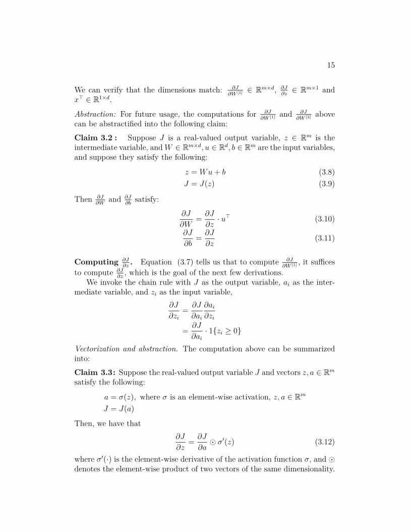
We can verify that the dimensions match: ∂J∂W [1] ∈ Rm×d, ∂J

∂z∈ Rm×1 and

x⊤ ∈ R1×d.

Abstraction: For future usage, the computations for ∂J∂W [1] and ∂J

∂W [2] abovecan be abstractified into the following claim:Claim 3.2 : Suppose J is a real-valued output variable, z ∈ Rm is theintermediate variable, and W ∈ Rm×d, u ∈ Rd, b ∈ Rm are the input variables,and suppose they satisfy the following:

z = Wu+ b (3.8)J = J(z) (3.9)

Then ∂J∂W

and ∂J∂b

satisfy:

∂J

∂W=

∂J

∂z· u⊤ (3.10)

∂J

∂b=

∂J

∂z(3.11)

Computing ∂J∂z

. Equation (3.7) tells us that to compute ∂J∂W [1] , it suffices

to compute ∂J∂z

, which is the goal of the next few derivations.We invoke the chain rule with J as the output variable, ai as the inter-

mediate variable, and zi as the input variable,∂J

∂zi=

∂J

∂ai

∂ai∂zi

=∂J

∂ai· 1{zi ≥ 0}

Vectorization and abstraction. The computation above can be summarizedinto:Claim 3.3: Suppose the real-valued output variable J and vectors z, a ∈ Rm

satisfy the following:

a = σ(z), where σ is an element-wise activation, z, a ∈ Rm

J = J(a)

Then, we have that∂J

∂z=

∂J

∂a⊙ σ′(z) (3.12)

where σ′(·) is the element-wise derivative of the activation function σ, and ⊙denotes the element-wise product of two vectors of the same dimensionality.

16

Computing ∂J∂a

. Now it suffices to compute ∂J∂a

. We invoke the chain rulewith J as the output variable, o as the intermediate variable, and ai as theinput variable,

∂J

∂ai=

∂J

∂o

∂o

∂ai

= (o− y) ·W [2]i (because o =

∑mi=1 W

[2]i ai + b[2])

Vectorization. In vectorized notation, we have

∂J

∂a= W [2]⊤ · (o− y) (3.13)

Abstraction. We now present a more general form of the computation above.

Claim 3.4 : Suppose J is a real-valued output variable, v ∈ Rm is theintermediate variable, and W ∈ Rm×d, u ∈ Rd, b ∈ Rm are the input variables,and suppose they satisfy the following:

v = Wu+ b

J = J(v)

Then,

∂J

∂u= W⊤∂J

∂v(3.14)

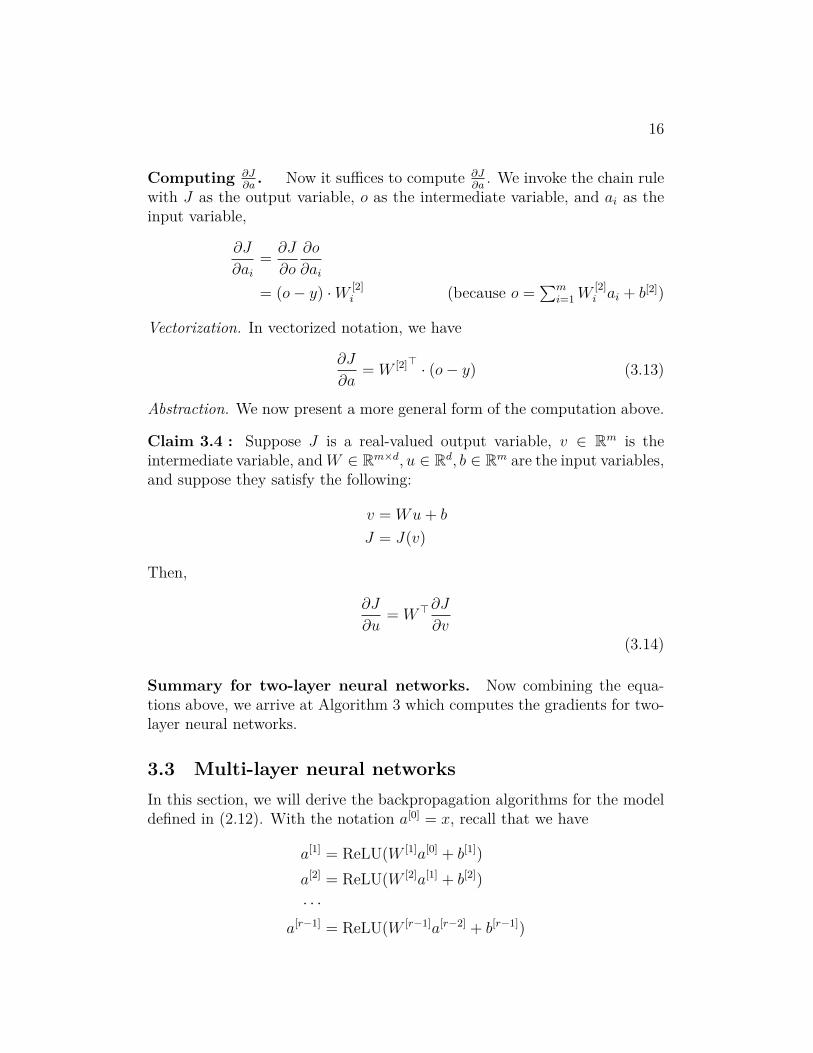
Summary for two-layer neural networks. Now combining the equa-tions above, we arrive at Algorithm 3 which computes the gradients for two-layer neural networks.

3.3 Multi-layer neural networksIn this section, we will derive the backpropagation algorithms for the modeldefined in (2.12). With the notation a[0] = x, recall that we have

a[1] = ReLU(W [1]a[0] + b[1])

a[2] = ReLU(W [2]a[1] + b[2])

· · ·a[r−1] = ReLU(W [r−1]a[r−2] + b[r−1])

17

Algorithm 3 Back-propagation for two-layer neural networks.1: Compute the values of z ∈ Rm, a ∈ Rm, and o ∈ R2: Compute

δ[2] ≜ ∂J

∂o= (o− y) ∈ R

δ[1] ≜ ∂J

∂z= (W [2]⊤(o− y))⊙ 1{z ≥ 0} ∈ Rm×1

(by eqn. (3.12) and (3.13))

3: Compute

∂J

∂W [2]= δ[2]a⊤ ∈ R1×m (by eqn. (3.5))

∂J

∂b[2]= δ[2] ∈ R (by eqn. (3.6))

∂J

∂W [1]= δ[1]x⊤ ∈ Rm×d (by eqn. (3.7))

∂J

∂b[1]= δ[1] ∈ Rm (as an exercise)

18

a[r] = z[r] = W [r]a[r−1] + b[r]

J =1

2(a[r] − y)2

Here we define both a[r] and z[r] as hθ(x) for notational simplicity.First, we note that we have the following local abstraction for k ∈

{1, . . . , r}:

z[k] = W [k]a[k−1] + b[k]

J = J(z[k])

Invoking Claim 3.2, we have that∂J

∂W [k]=

∂J

∂z[k]· a[k−1]⊤

∂J

∂b[k]=

∂J

∂z[k](3.15)

Therefore, it suffices to compute ∂J∂z[k]

. For simplicity, let’s define δ[k] ≜ ∂J∂z[k]

.We compute δ[k] from k = r to 1 inductively. First we have that

δ[r] ≜ ∂J

∂z[r]= (z[r] − y) (3.16)

Next for k ≤ r − 1, suppose we have computed the value of δ[k+1], then wewill compute δ[k]. First, using Claim 3.3, we have that

δ[k] ≜ ∂J

∂z[k]=

∂J

∂a[k]⊙ ReLU′(z[k])

Then we note that the relationship between a[k] and z[k+1] can be abstractlywritten as

z[k+1] = W [k+1]a[k] + b[k+1] (3.17)J = J(z[k+1]) (3.18)

Therefore by Claim 3.4 we have that∂J

∂a[k]= W [k+1]⊤ ∂J

∂z[k+1](3.19)

It follows that

δ[k] =

(W [k+1]⊤ ∂J

∂z[k+1]

)⊙ ReLU′(z[k])

=(W [k+1]⊤δ[k+1]

)⊙ ReLU′(z[k])

19

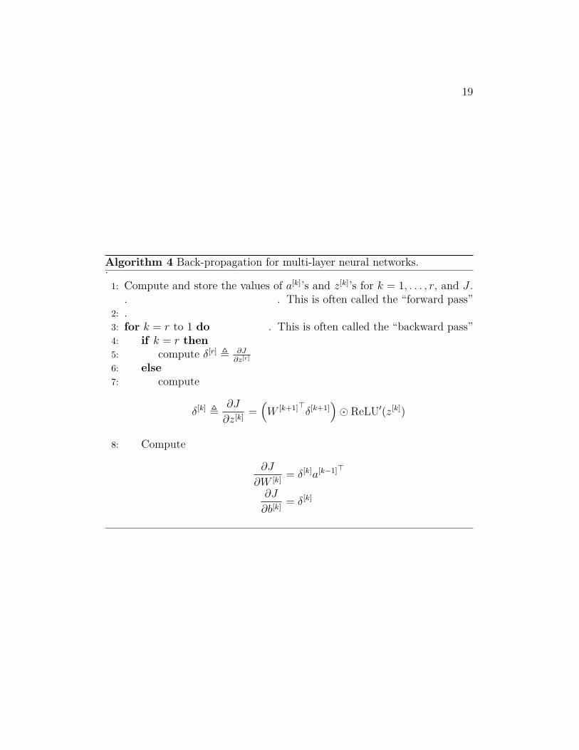
Algorithm 4 Back-propagation for multi-layer neural networks..1: Compute and store the values of a[k]’s and z[k]’s for k = 1, . . . , r, and J .

. ▷ This is often called the “forward pass”2: .3: for k = r to 1 do ▷ This is often called the “backward pass”4: if k = r then5: compute δ[r] ≜ ∂J

∂z[r]

6: else7: compute

δ[k] ≜ ∂J

∂z[k]=

(W [k+1]⊤δ[k+1]

)⊙ ReLU′(z[k])

8: Compute

∂J

∂W [k]= δ[k]a[k−1]⊤

∂J

∂b[k]= δ[k]

20

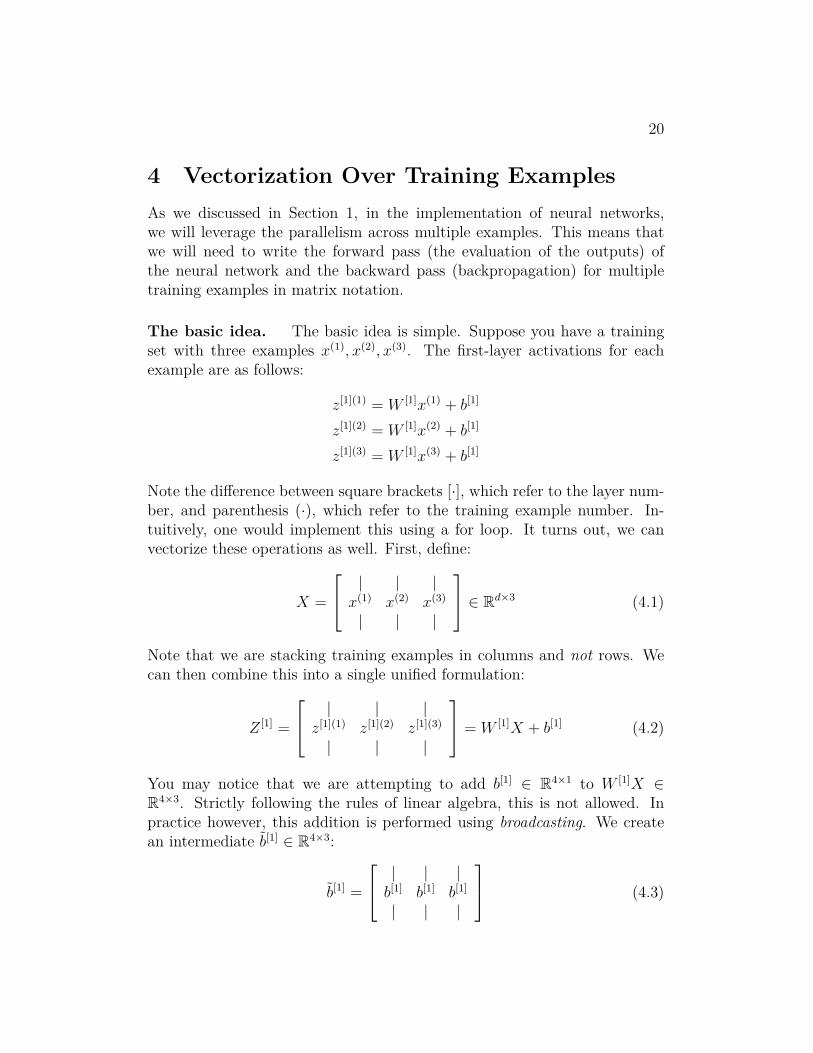
4 Vectorization Over Training ExamplesAs we discussed in Section 1, in the implementation of neural networks,we will leverage the parallelism across multiple examples. This means thatwe will need to write the forward pass (the evaluation of the outputs) ofthe neural network and the backward pass (backpropagation) for multipletraining examples in matrix notation.

The basic idea. The basic idea is simple. Suppose you have a trainingset with three examples x(1), x(2), x(3). The first-layer activations for eachexample are as follows:

z[1](1) = W [1]x(1) + b[1]

z[1](2) = W [1]x(2) + b[1]

z[1](3) = W [1]x(3) + b[1]

Note the difference between square brackets [·], which refer to the layer num-ber, and parenthesis (·), which refer to the training example number. In-tuitively, one would implement this using a for loop. It turns out, we canvectorize these operations as well. First, define:

X =

| | |x(1) x(2) x(3)

| | |

∈ Rd×3 (4.1)

Note that we are stacking training examples in columns and not rows. Wecan then combine this into a single unified formulation:

Z [1] =

| | |z[1](1) z[1](2) z[1](3)

| | |

= W [1]X + b[1] (4.2)

You may notice that we are attempting to add b[1] ∈ R4×1 to W [1]X ∈R4×3. Strictly following the rules of linear algebra, this is not allowed. Inpractice however, this addition is performed using broadcasting. We createan intermediate b̃[1] ∈ R4×3:

b̃[1] =

| | |b[1] b[1] b[1]

| | |

(4.3)

21

We can then perform the computation: Z [1] = W [1]X + b̃[1]. Often times, itis not necessary to explicitly construct b̃[1]. By inspecting the dimensions in(4.2), you can assume b[1] ∈ R4×1 is correctly broadcast to W [1]X ∈ R4×3.

The matricization approach as above can easily generalize to multiplelayers, with one subtlety though, as discussed below.

Complications/Subtlety in the Implementation. All the deep learn-ing packages or implementations put the data points in the rows of a datamatrix. (If the data point itself is a matrix or tensor, then the data are con-centrated along the zero-th dimension.) However, most of the deep learningpapers use a similar notation to these notes where the data points are treatedas column vectors.7 There is a simple conversion to deal with the mismatch:in the implementation, all the columns become row vectors, row vectors be-come column vectors, all the matrices are transposed, and the orders of thematrix multiplications are flipped. In the example above, using the row ma-jor convention, the data matrix is X ∈ R3×d, the first layer weight matrixhas dimensionality d × m (instead of m × d as in the two layer neural netsection), and the bias vector b[1] ∈ R1×m. The computation for the hiddenactivation becomes

Z [1] = XW [1] + b[1] ∈ R3×m (4.4)

7The instructor suspects that this is mostly because in mathematics we naturally multiplya matrix to a vector on the left hand side.