Deep learning seismic facies on state-of-the-art CNN architecturesJesper S. Dramsch∗, Technical University of Denmark, and Mikael Luthje, Technical University of Denmark

SUMMARY

We explore propagation of seismic interpretation by deeplearning in stacked 2D sections. We show the applicationof state-of-the-art image classification algorithms on seismicdata. These algorithms were trained on big labeled photographdatabases. We use transfer learning to benefit from pre-trainednetworks and evaluate their performance on seismic data.

INTRODUCTION

Seismic interpretation is often dependent on the interpretersexperience and knowledge. While deep learning cannot re-place expert knowledge, we explore the accuracy of convolu-tional networks in interpreting seismic data to support humaninterpretation.

In the 1950s neural networks started as a simple direct con-nection of several nodes in an input layer to several nodes inan output layer (Widrow and Lehr, 1990). In geophysics thisputs us to the introduction of seismic trace stacking (Yilmaz,2001). In 1989 the first idea of a convolutional neural networkwas born (Lecun, 1989) and back-propagation was formalizedas an error-propagation mechanism (Rumelhart et al., 1988).In 2012 the paper (Krizhevsky et al., 2012) propelled the fieldof deep learning forward implementing essential components,namely GPU training, ReLu activation functions (Dahl et al.,2013) and dropout (Srivastava et al., 2014). They outperformedprevious models in the ImageNet challenge (Deng et al., 2009)by almost halving the prediction error. Waldeland and Solberg(2016) showed that neural networks can be used to classify saltdiapirs in 3D seismic data. Charles Rutherford Ildstad (2017)generalized this work to nD and beyond two classes of salt and”else”.

The task of automatic seismic interpretation can be equated todense object detection (Lin et al., 2017) or semantic segmen-tation. These tasks are currently best solved by Mask R-CNNarchitectures (Long et al., 2015). Statoil has used U-Nets forautomatic seismic interpretation. Yet, classification networkscan be used for semantic segmentation, but are significantlyslower. The benefit is a testable example of generalization ofpre-trained networks form photographic data to seismic im-ages. As well as, a testable framework for choosing hyper-parameters for neural networks on seismic data.

Deep learning relies heavily on vast amounts of labeled datato train on initially. However, the features learned from thesenetworks can often be transferred to adjacent problem spaces(Baxter, 1998). Often these transfer learning tasks are tested onphotographs rather than seismic or medical imaging tasks. Theaim of this study is to evaluate state-of-the-art pre-trained net-works in the task of automatic seismic interpretation. We com-pare three convolutional neural networks of increasing com-

plexity in the task of supervised automatic seismic interpreta-tion. We evaluate these tasks qualitatively and quantitatively.

METHODS

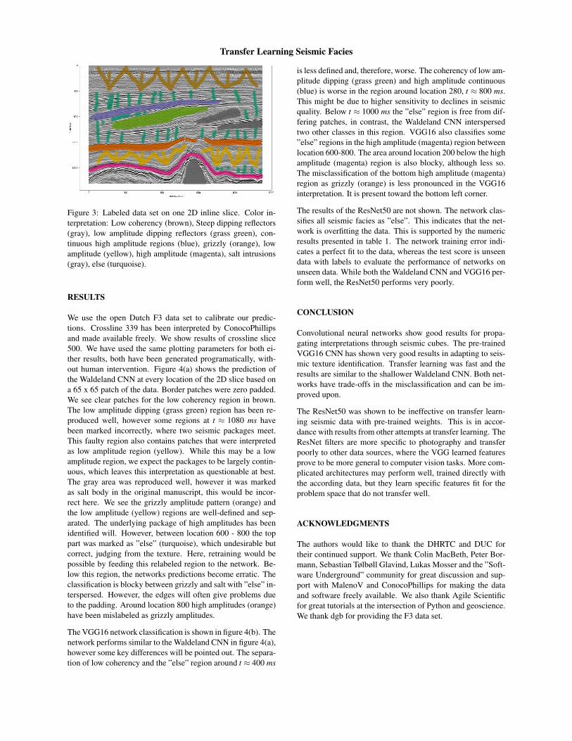
The neural networks in this study learn supervised. The fea-tures were published alongside the open source frameworkMalenoV and describe nine seismic facies in the open F3 dataset. The classes describe steep dipping reflectors, salt intru-sions, low coherency regions, low amplitude dipping reflec-tors, high amplitude regions continuous high amplitude re-gions and grizzly amplitude patterns presented in figure 3. Ad-ditionally, a catch-all “else” region are picked. In this approachwe chose Keras (Chollet et al., 2015) with a Tensorflow (Abadiet al., 2015) backend on a K5200 GPU at DHRTC. Keras is apowerful high level abstraction of tensor arithmetics. Tensor-flow is an open source numerical computation library on staticgraphs. We train 2D convolutional neural networks (CNN) ofvarying depth on seismic slices to propagate single slice inter-pretations to a volume. CNNs are highly flexible models forcomputer vision tasks.

Network one depicted in figure 2 was developed by Walde-land and Solberg (2016) to identify salt bodies in 3D seis-mic data. Three layers are fully connected for classification.The network uses a kernel of 5 by 5 pixels for convolutionand a stride of 2 for down-sampling. We use the Adam op-timizer and cross-categorical entropy as a loss function. TheAdam optimizer is an extension to stochastic gradient descent(SGD) that implements adaptive learning rates and bias cor-rection (Ruder, 2016). We add dropout and batch normaliza-tion to the network. These methods improve regularizationand prevent overfitting. Furthermore, we use early-stopping toprevent overfitting the model by over-training. We chose twometrics to monitor in the training and validation sets, namelymean absolute error and accuracy. The Waldeland CNN is rel-atively shallow compared to modern deep learning networkswith 95,735 parameters to optimize for.

Network two is the VGG16 network (Simonyan and Zisser-man, 2014) by the Visual Geometry Group. It contains 16layers and 1,524,2605 parameters. 13 of these layers ore con-volutional layers with a 3x3 kernel. Convolutional blocks areinterspersed with max-pooling layers for down-sampling. Thelast three layers are fully connected layers for classification.The VGG16 architecture was proposed for the ImageNet chal-lenge in 2013. It is widely used for it’s simplicity in teachingand it’s generalizability in transfer learning tasks.

Network three is the ResNet50 architecture by Microsoft. Thenetwork consists of 50 layers with 2,361,6569 parameters. Itimplements a recent development, called residual blocks. Theseresidual blocks add a skip- or identity-connection around astack of 1x1, 3x3, 1x1 convolutional layers (He et al., 2016).The 1x1 are identity convolutions, used for down- and subse-

Transfer Learning Seismic Facies

Figure 1: Waldeland CNN architecture. Input at the Top. Soft-max Classification Layer on bottom. Width of objects showslog of spatial extent of layer. Height shows log of complexityof layer. The layers are color coded to show similar purpose.

quent up-sampling to decrease the computational cost of verydeep CNNs. The convolutional layers are followed by onefully connected layer for classification.

All networks use rectified linear units (ReLu) as neural acti-vation. The last layer uses Softmax as activation to outputa probability for each class. Training both VGG16 and theResNet50 end to end would be very expensive. These mod-els have been trained on big labeled data that are not availablein geoscience. However, transfer learning enables us to usepre-trained networks on very different tasks. In transfer learn-ing, we use the learned weights of the networks and replacethe fully connected layers. These untrained layers are specificto our task and have to be fine-tuned to the data. This pro-cess is very fast and requires little data. We fine-tune an entirenetwork on one sparsely interpreted 2D seismic slice. For thefine-tuning process, we replace the Adam optimizer by a clas-sic SGD optimizer with lower learning rate, very low weightdecay and Nesterov momentum. We still use early-stoppingon validation loss and cross-categorical entropy.

Figure 2: VGG16 architecture. Same visualization as figure 2

We added the same fully connected layer architecture to VGG16and ResNet50 that Waldeland added to their architecture. There-fore, we test if pre-trained convolution kernels are fit to rec-ognize texture features in seismic data. We set up a valida-tion set to quantify the accuracy of our networks on previouslyunseen data. Additionally, we set up a prediction pipeline topopulate each one 2D inline and crossline of the seismic datato qualitatively visualize the prediction capability of the net-works. The labels for the supervised interpretation are takenfrom the MalenoV interpretation by ConocoPhillips, shown infigure 3.

Network Run Loss MAE Acc

Waldeland CNNTraining 0.001 0.000 100.0%Test 0.003 0.000 99.9%

VGG16Training 0.010 0.005 99.8%Test 0.127 0.026 100.0%

ResNet50Training 0.011 0.001 100.0%Test 14.166 0.195 12.1%

Table 1: Training and Test scores on Networks. Test scores areprediction results on a labeled hold-out data set. Mismatch oftest and training scores indicates over-fitting.

Transfer Learning Seismic Facies

Figure 3: Labeled data set on one 2D inline slice. Color in-terpretation: Low coherency (brown), Steep dipping reflectors(gray), low amplitude dipping reflectors (grass green), con-tinuous high amplitude regions (blue), grizzly (orange), lowamplitude (yellow), high amplitude (magenta), salt intrusions(gray), else (turquoise).

RESULTS

We use the open Dutch F3 data set to calibrate our predic-tions. Crossline 339 has been interpreted by ConocoPhillipsand made available freely. We show results of crossline slice500. We have used the same plotting parameters for both ei-ther results, both have been generated programatically, with-out human intervention. Figure 4(a) shows the prediction ofthe Waldeland CNN at every location of the 2D slice based ona 65 x 65 patch of the data. Border patches were zero padded.We see clear patches for the low coherency region in brown.The low amplitude dipping (grass green) region has been re-produced well, however some regions at t ≈ 1080 ms havebeen marked incorrectly, where two seismic packages meet.This faulty region also contains patches that were interpretedas low amplitude region (yellow). While this may be a lowamplitude region, we expect the packages to be largely contin-uous, which leaves this interpretation as questionable at best.The gray area was reproduced well, however it was markedas salt body in the original manuscript, this would be incor-rect here. We see the grizzly amplitude pattern (orange) andthe low amplitude (yellow) regions are well-defined and sep-arated. The underlying package of high amplitudes has beenidentified will. However, between location 600 - 800 the toppart was marked as ”else” (turquoise), which undesirable butcorrect, judging from the texture. Here, retraining would bepossible by feeding this relabeled region to the network. Be-low this region, the networks predictions become erratic. Theclassification is blocky between grizzly and salt with ”else” in-terspersed. However, the edges will often give problems dueto the padding. Around location 800 high amplitudes (orange)have been mislabeled as grizzly amplitudes.

The VGG16 network classification is shown in figure 4(b). Thenetwork performs similar to the Waldeland CNN in figure 4(a),however some key differences will be pointed out. The separa-tion of low coherency and the ”else” region around t ≈ 400 ms

is less defined and, therefore, worse. The coherency of low am-plitude dipping (grass green) and high amplitude continuous(blue) is worse in the region around location 280, t ≈ 800 ms.This might be due to higher sensitivity to declines in seismicquality. Below t ≈ 1000 ms the ”else” region is free from dif-fering patches, in contrast, the Waldeland CNN interspersedtwo other classes in this region. VGG16 also classifies some”else” regions in the high amplitude (magenta) region betweenlocation 600-800. The area around location 200 below the highamplitude (magenta) region is also blocky, although less so.The misclassification of the bottom high amplitude (magenta)region as grizzly (orange) is less pronounced in the VGG16interpretation. It is present toward the bottom left corner.

The results of the ResNet50 are not shown. The network clas-sifies all seismic facies as ”else”. This indicates that the net-work is overfitting the data. This is supported by the numericresults presented in table 1. The network training error indi-cates a perfect fit to the data, whereas the test score is unseendata with labels to evaluate the performance of networks onunseen data. While both the Waldeland CNN and VGG16 per-form well, the ResNet50 performs very poorly.

CONCLUSION

Convolutional neural networks show good results for propa-gating interpretations through seismic cubes. The pre-trainedVGG16 CNN has shown very good results in adapting to seis-mic texture identification. Transfer learning was fast and theresults are similar to the shallower Waldeland CNN. Both net-works have trade-offs in the misclassification and can be im-proved upon.

The ResNet50 was shown to be ineffective on transfer learn-ing seismic data with pre-trained weights. This is in accor-dance with results from other attempts at transfer learning. TheResNet filters are more specific to photography and transferpoorly to other data sources, where the VGG learned featuresprove to be more general to computer vision tasks. More com-plicated architectures may perform well, trained directly withthe according data, but they learn specific features fit for theproblem space that do not transfer well.

ACKNOWLEDGMENTS

The authors would like to thank the DHRTC and DUC fortheir continued support. We thank Colin MacBeth, Peter Bor-mann, Sebastian Tølbøll Glavind, Lukas Mosser and the ”Soft-ware Underground” community for great discussion and sup-port with MalenoV and ConocoPhillips for making the dataand software freely available. We also thank Agile Scientificfor great tutorials at the intersection of Python and geoscience.We thank dgb for providing the F3 data set.

Transfer Learning Seismic Facies

((a)) Waldeland CNN automatic interpretation of crossline 500.

((b)) VGG16 automatic interpretation of crossline 500.

Figure 4: Automatic seismic interpretation with CNNs. Color interpretation: Low coherency (brown), Steep dipping reflectors(gray), low amplitude dipping reflectors (grass green), continuous high amplitude regions (blue), grizzly (orange), low amplitude(yellow), high amplitude (magenta), salt intrusions (gray), else (turquoise).

Transfer Learning Seismic Facies

REFERENCES

Abadi, M., A. Agarwal, P. Barham, E. Brevdo, Z. Chen, C.Citro, G. S. Corrado, A. Davis, J. Dean, M. Devin, S. Ghe-mawat, I. Goodfellow, A. Harp, G. Irving, M. Isard, Y.Jia, R. Jozefowicz, L. Kaiser, M. Kudlur, J. Levenberg, D.Mane, R. Monga, S. Moore, D. Murray, C. Olah, M. Schus-ter, J. Shlens, B. Steiner, I. Sutskever, K. Talwar, P. Tucker,V. Vanhoucke, V. Vasudevan, F. Viegas, O. Vinyals, P. War-den, M. Wattenberg, M. Wicke, Y. Yu, and X. Zheng, 2015,TensorFlow: Large-scale machine learning on heteroge-neous systems. (Software available from tensorflow.org).

Baxter, J., 1998, Theoretical models of learning to learn, inLearning to learn: Springer, 71–94.

Charles Rutherford Ildstad, P. B., 2017, MalenoV. Machinelearning of Voxels.

Chollet, F., et al., 2015, Keras:https://github.com/fchollet/keras.

Dahl, G. E., T. N. Sainath, and G. E. Hinton, 2013, Improvingdeep neural networks for LVCSR using rectified linear unitsand dropout: Presented at the 2013 IEEE International Con-ference on Acoustics Speech and Signal Processing, IEEE.

Deng, J., W. Dong, R. Socher, L.-J. Li, K. Li, and L. Fei-Fei, 2009, ImageNet: A Large-Scale Hierarchical ImageDatabase: Presented at the CVPR09.

He, K., X. Zhang, S. Ren, and J. Sun, 2016, Deep residuallearning for image recognition: Proceedings of the IEEEconference on computer vision and pattern recognition,770–778.

Krizhevsky, A., I. Sutskever, and G. E. Hinton, 2012, Ima-geNet Classification with Deep Convolutional Neural Net-works, in Advances in Neural Information Processing Sys-tems 25: Curran Associates, Inc., 1097–1105.

Lecun, Y., 1989, Generalization and network design strategies,in Connectionism in perspective: Elsevier. (Accessed onMon, November 20, 2017).

Lin, T.-Y., P. Goyal, R. Girshick, K. He, and P. Dollar,2017, Focal loss for dense object detection: arXiv preprintarXiv:1708.02002.

Long, J., E. Shelhamer, and T. Darrell, 2015, Fully convolu-tional networks for semantic segmentation: Proceedings ofthe IEEE conference on computer vision and pattern recog-nition, 3431–3440.

Ruder, S., 2016, An overview of gradient descent optimizationalgorithms: arXiv preprint arXiv:1609.04747.

Rumelhart, D., G. Hinton, and R. Williams, 1988, LearningInternal Representations by Error Propagation, in Readingsin Cognitive Science: Elsevier, 399–421.

Simonyan, K., and A. Zisserman, 2014, Very deep convolu-tional networks for large-scale image recognition: arXivpreprint arXiv:1409.1556.

Srivastava, N., G. Hinton, A. Krizhevsky, I. Sutskever, andR. Salakhutdinov, 2014, Dropout: A Simple Way to Pre-vent Neural Networks from Overfitting: Journal of MachineLearning Research, 15, 1929–1958.

Waldeland, A., and A. Solberg, 2016, 3D Attributes and Clas-sification of Salt Bodies on Unlabelled Datasets: Presentedat the 78th EAGE Conference and Exhibition 2016, EAGEPublications BV.

Widrow, B., and M. Lehr, 1990, 30 years of adaptive neuralnetworks: perceptron Madaline, and backpropagation: Pro-ceedings of the IEEE, 78, 1415–1442.

Yilmaz, O., 2001, Seismic Data Analysis: Society of Explo-ration Geophysicists.