Deep Learning of Visual Control Policies - UCL/ELEN - … · Deep Learning of Visual Control...

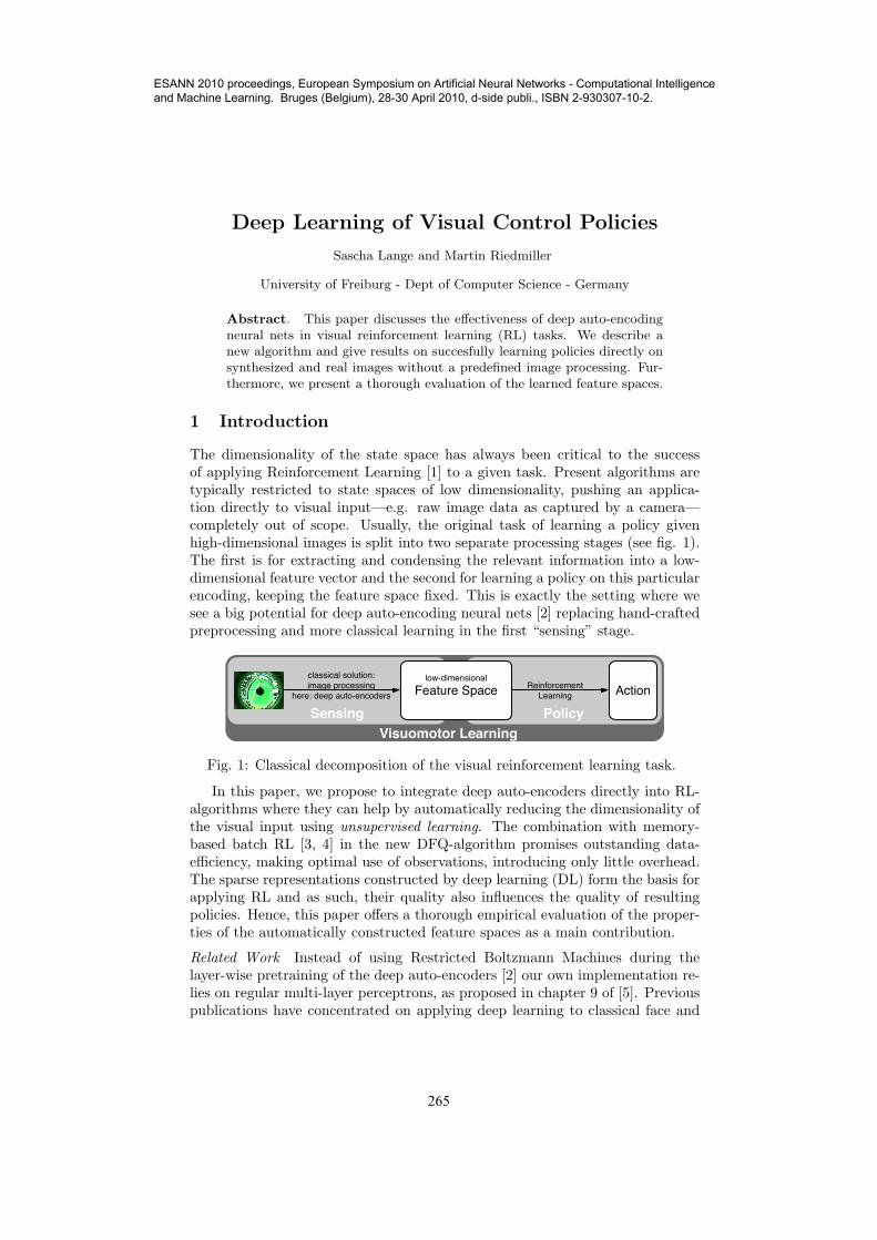
Deep Learning of Visual Control Policies

Sascha Lange and Martin Riedmiller

University of Freiburg - Dept of Computer Science - Germany

Abstract. This paper discusses the effectiveness of deep auto-encodingneural nets in visual reinforcement learning (RL) tasks. We describe anew algorithm and give results on succesfully learning policies directly onsynthesized and real images without a predefined image processing. Fur-thermore, we present a thorough evaluation of the learned feature spaces.

1 Introduction

The dimensionality of the state space has always been critical to the successof applying Reinforcement Learning [1] to a given task. Present algorithms aretypically restricted to state spaces of low dimensionality, pushing an applica-tion directly to visual input—e.g. raw image data as captured by a camera—completely out of scope. Usually, the original task of learning a policy givenhigh-dimensional images is split into two separate processing stages (see fig. 1).The first is for extracting and condensing the relevant information into a low-dimensional feature vector and the second for learning a policy on this particularencoding, keeping the feature space fixed. This is exactly the setting where wesee a big potential for deep auto-encoding neural nets [2] replacing hand-craftedpreprocessing and more classical learning in the first “sensing” stage.

Policy

low-dimensionalFeature Space

Action

classical solution:image processing

here: deep auto-encodersReinforcement

Learning

SensingVisuomotor Learning

Fig. 1: Classical decomposition of the visual reinforcement learning task.

In this paper, we propose to integrate deep auto-encoders directly into RL-algorithms where they can help by automatically reducing the dimensionality ofthe visual input using unsupervised learning. The combination with memory-based batch RL [3, 4] in the new DFQ-algorithm promises outstanding data-efficiency, making optimal use of observations, introducing only little overhead.The sparse representations constructed by deep learning (DL) form the basis forapplying RL and as such, their quality also influences the quality of resultingpolicies. Hence, this paper offers a thorough empirical evaluation of the proper-ties of the automatically constructed feature spaces as a main contribution.

Related Work Instead of using Restricted Boltzmann Machines during thelayer-wise pretraining of the deep auto-encoders [2] our own implementation re-lies on regular multi-layer perceptrons, as proposed in chapter 9 of [5]. Previouspublications have concentrated on applying deep learning to classical face and

265

ESANN 2010 proceedings, European Symposium on Artificial Neural Networks - Computational Intelligence and Machine Learning. Bruges (Belgium), 28-30 April 2010, d-side publi., ISBN 2-930307-10-2.

letter recognition tasks [2, 5]. The RL-tasks studied here also add the complexityof tracking moving objects and encoding their positions adequately.

[3] was the first attempt of applying model-based batch RL directly to(synthesized) images. Following the classical decompositional approach, in [6]Jodogne tried to further integrate the construction of feature spaces into RL butsucceeded only in learning the selection—not the extraction—of the features.Both [3, 6] lacked realistic images, ignored noise and just learned to memorize afinite set of observations, not testing for generalization at all.

2 RL on image data: Deep Fitted Q-Iteration

In the general reinforcement learning setting [1], an agent interacts with anenvironment in discrete time steps t, observing some markovian state st ∈ Sand reward rt to then respond with an action at ∈ A. The task is to learn astationary policy π : S 7→ A that maximizes the expectation of the discountedsum of rewards Rt =

∑∞k=0 γ

trt+k+1 with discount factor γ ∈ [0, 1]. A standardsolution is learning the optimal q-function Q∗(s, a) = E[Rt|st = s, at = a] thatspecifies the expected reward when always selecting the optimal action startingwith t+ 1 and then deriving the optimal policy π∗ by greedy evaluation [1].

In the tasks considered here, the learner does not know anything about thesystem state but only observes a high-dimensional image ot ∈ [0, 1]d. The ob-servations ot are assumed to be markov1. The new idea followed here is tointegrate the unsupervised training of deep auto-encoders into Ernst’s fittedq-iteration (FQI) [4] in order to obtain an encoding of the images in a low-dimensional feature space. Due to space limitations, we will only briefly discussthe basic version of the new algorithm “deep fitted q-iteration” (DFQ) and mayrefer the reader to [7] for a more thorough treatment of batch RL in general.

A. Initialization Set k ← 0. Set p ← 0. Create an initial (random) explorationstrategy π0 : z 7→ a and an inital encoder ENC : o 7→W0 z with (random) weightvector W 0. Start with an empty set FO = � of transitions (ot, at, rt+1,ot+1)

B. Episodic Exploration In each time step t calculate the feature vector zt fromthe observed image ot by using the present encoder zt = ENC(ot;W

k). Se-lect an action at ← πk(zt) and store the completed transition FO ← FO ∪(op, ap, rp+1,op+1) incrementing p with each observed transition.

C. Encoder Training Train an auto-encoder on the p observations in FO using re-silient propagation during layer-wise pretraining and finetuning. Derive the en-coder ENC( · ;W k+1) (first half of the auto-encoder, see [2]). Set k ← k + 1

D. Encoding Apply the encoder ENC(o;W k) to all (ot, at, rt+1,ot+1) ∈ FO, trans-fering the transitions into the feature space Z, constructing a set FZ ={(zt, at, rt+1, zt+1)| t = 1, . . . , p} with zt = ENC(ot;W

k).

E. Inner Loop: FQI Call FQI with FZ . Starting with an initial approximationQ0(z, a) = 0 ∀(z, a) ∈ Z × A FQI (details in [4]) iterates over a dynamicprogramming step creating a training set Pi+1 = {(zt, at; q

i+1t )|t = 1, ..., p} with

1This does hold for a system that generates different observations o for exactly the samestate s (e.g. due to noise) but never produces the same observation for two different states.

266


qi+1t = rt+1 + γmaxa′∈A Q

i(zt+1, a′) and a supervised learning step training a

function approximator on P i+1, obtaining the approximated Q-function Qi+1.

F. Outer loop If satisfied or if running in pure batch mode without recurring ex-ploration, return approximation Qi, greedy policy π and encoder ENC(o;W k).Otherwise derive an exploration strategy πk from Qi and continue with step B.

In the outer loop, the learner uses the present approximation of the q-functionto derive a policy—e.g. by ε-greedy evaluation [1]—for collecting further expe-rience. In the inner loop, the agent uses the present encoder to translate allcollected observations to the feature space and then applies FQI to improvean approximation of the q-function. Each time a new encoder ENC(·;W k+1)is learned in C, thus the feature space is changed, the approximation of theq-function and the derived policy become invalid. Whereas online-RL wouldhave to start calculating the q-function completely from scratch, in the batchapproach the stored transitions can be used to immediately calculate a newq-function in the new feature space, without any further interaction.

When using an averager [3] or kernel-based approximator [8] for approxi-mating the q-function, the series of approximations {Qi} produced by the FQIalgorithm—under some assumptions—is guaranteed to converge to a q-functionQ that is within a specific bound of the optimal q-function Q∗ [4, 8]. Sincethe non-linear encoding ENC : O 7→ Z does not change during the inner loop,these results also cover applying the FQI algorithm to the feature vectors. Theweights of the averager or kernel theoretically can be adapted to include thenon-linear mapping as well, as the only restriction on the weights is summingup to 1 [3, 8]. The remaining problem is the bound on the distance ||Q∗ − Q||∞[8] that—by “hiding” the encoding in the weights—becomes dependent on theparticular encoding. Since, there are no helpful formal results on the propertiesof the feature spaces learned by DL, the best to do is an empirical evaluation.

3 Results

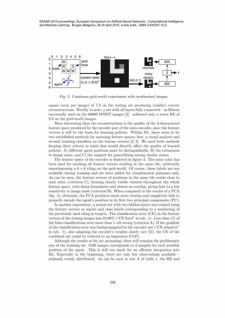
We evaluated the algorithm on a continuous grid-world problem using synthe-sized images (see fig. 2). Instead of the internal system state (x, y) ∈ [0, 6)2, theagent receives only a rendered image with 30-pixels and added gaussian noiseN (0, 0.1). Due to the discrete nature of the pixels, the number of possible agentpositions is limited to 900. Each action moves the agent 1m in the selecteddirection. The task of reaching the goal has been modeled as a shortest-pathproblem [1], with a reward of -1 for any transition outside the goal area.

After testing several topologies on a set of 3100 evenly-distributed trainingimages and as many testing images, we have selected a rather huge auto-encoderwith 21 layers in total and receptive fields2 of 9×9 neurons in the four outermostlayers, otherwise being fully connected between adjacent layers. This net withmore than 350 000 weights achieved the best reconstruction error (RE, mean

2The method of connecting only a number of neighbouring neurons to a neuron of thesubsequent layer has some motivation in biology and dates back at least to the neocognitron.

267


WW GW W W

A

0 1 2 3 4 5

543210

S

WE

N

5px

6

6W goal

area

agent

walls

system state(x,y) ∈ [0,6)2 N(0,0.1)

900

900

2...

...

noisyobserv.

reconstr.z

Fig. 2: Continous grid-world experiment with synthesized images.

square error per image) of 7.3 on the testing set producing (visibly) correctreconstructions. Worthy to note, a net with all layers fully connected—as Hintonsuccessully used on the 60000 MNIST images [2]—achieved only a worse RE of9.8 on the grid-world images.

More interesting than the reconstructions is the quality of the 2-dimensionalfeature space produced by the encoder part of the auto-encoder, since the featurevectors z will be the basis for learning policies. Within DL, there seem to betwo established methods for assessing feature spaces; first, a visual analysis andsecond, training classifiers on the feature vectors [2, 5]. We used both methodskeeping three criteria in mind that would directly affect the quality of learnedpolicies: A) different agent positions must be distinguishable, B) the robustnessto image noise, and C) the support for generalizing among similar states.

The feature space of the encoder is depicted in figure 3. The same color hasbeen used for marking all feature vectors residing in the same tile, arbitrarilysuperimposing a 6 × 6 tiling on the grid-world. Of course, these labels are notavailable during training and are later added for visualtization purposes only.As can be seen, the feature vectors of positions in the same tile reside close toeach other (criterion C), forming clearly visible clusters throughout the wholefeature space, with sharp boundaries and almost no overlap, giving hint to a lowsensitivity to image noise (criterion B). When compared to the results of a PCA(fig. 4), obviously, the PCA produces much more overlap and completely fails toproperly encode the agent’s position in its first two principal components (PC).

In another experiment, a neural net with two hidden layers was trained usingthe feature vectors as inputs and class labels corresponding to a numbering ofthe previously used tiling as targets. The classification error (CE) on the featurevectors of the testing images was 19.90% (“CE fixed” in tab. 1). Less than 1% ofthe false-classifications were more than 1 cell wrong (criterion A). If the gradientof the classification error was backpropagated in the encoder net (“CE adaptive”in tab. 1), also adapting the encoder’s weights slowly (see [2]), the CE of thecombined net could be reduced to an impressive 0.54%.

Although the results so far are promising, there still remains the problematicsize of the training set. 3100 images corresponds to 4 samples for each possibleposition of the agent. This is still too much for an efficient integration intoRL. Especially in the beginning, there are only few observations available—seldomly evenly distributed. As can be seen in row A of table 1, the RE and

268


Table 1: Reconstruction errors (RE) and classification errors (CE) for differntsizes of the training set Row A: receptive fields. Row B: convolutional kernels.For comparison reasons: results of a PCA in the last column (using 2 PCs).

Samples 7→ 155 465 775 1550 3100 3100

RE 27.58 18.9 12.0 9.4 7.3 15.80A CE Fixed 75.48% 62.69% 40.39% 38.58% 19.90% 60.42%

CE Adaptiv 74.19% 59.14% 19.13% 8.41% 0.54% –

RE 12.38 9.42 7.8 7.6 6.8 –B CE Fixed 36.13% 28.17% 17.29% 17.03% 11.23% –

CE Adaptiv 35.48% 12.25% 7.61% 0.13% 0.0% –

0.1

0.2

0.3

0.4

0.5

0.6

0.7

0.8

0.9

0 0.1 0.2 0.3 0.4 0.5 0.6 0.7 0.8 0.9 0

0.1

0.2

0.3

0.4

0.5

0.6

0.7

0.8

0.9

1

0 0.1 0.2 0.3 0.4 0.5 0.6 0.7 0.8 0.9 1

0.1

0.2

0.3

0.4

0.5

0.6

0.7

0.8

0.9

0 0.1 0.2 0.3 0.4 0.5 0.6 0.7 0.8 0.9 1 0

0.1

0.2

0.3

0.4

0.5

0.6

0.7

0.8

0.9

0 0.1 0.2 0.3 0.4 0.5 0.6 0.7 0.8 0.9 1

0

0.1

0.2

0.3

0.4

0.5

0.6

0.7

0.8

0.9

0 0.1 0.2 0.3 0.4 0.5 0.6 0.7 0.8 0.9 1

after pretraining 20 epochs 40 epochs

100 epochs

400 epochs

0

0.1

0.2

0.3

0.4

0.5

0.6

0.7

0.8

0.9

1

0 0.1 0.2 0.3 0.4 0.5 0.6 0.7 0.8 0.9 1

200 epochs

Fig. 3: Evolution of the feature space during finetuning the auto-encoder.

1 2 3 4 10 100

PCADL Orig

n-th PC

-2

-1.5

-1

-0.5

0

0.5

1

1.5

2

-2 -1.5 -1 -0.5 0 0.5 1 1.5 2

Fig. 4: Eigenimages of some PCs found by PCA (top row) and reconstructionof the original image (“Orig”) when using the n first PCs or DL (left of Orig).

CE quickly degrades when the number of samples is further reduced. For thosesmall training sets, the results can be greatly enhanced by using weight sharingand convolutional kernels replacing the (independent) receptive fields [9] (rowB). Even in the case of only 155 random distributed training samples (that is acovering of the possible agent positions by only 20%) the CE of < 40% is betterthan the result of the receptive fields when training on a 100% covering.

Learning a policy We started the DFQ-algorithm from scratch and let it learna policy by interacting with the grid-world. Every few episodes a new encoderwas trained in the outer loop, using 9× 9 convolutional kernels. The q-functionwas approximated using a regular-grid approximator with 20 × 20 cells. Thebest policy within 500 episodes (maximal length of 20 steps, 3795 steps in total)

269


achieved an average reward (AR) of −5.42, what is within half a step of theoptimal policy. During the last 100 episodes the AR was very stable (σ = 0.01).

Finally, we repeated the same experiment with a real image-formation pro-cess: the grid-world was plotted on a computer monitor and captured in real-time (10 Hz) using a video camera. DFQ received a sub-sampled version (40×30pixels, no smooting) of the captured QVGA-image and had to handle real im-age noise, slight barrel distortion and non-uniform lighting conditions. After44 episodes the learned policy reached the goal from 50% of the tested startingstates collecting an average reward of −11.53. The best policy (episode 492) hadan AR of −5.53, only slightly below the simulation.

4 Discussion

We have presented the new DFQ algorithm for efficiently learning near-optimalpolicies on visual input. The evaluation of the feature spaces has shown deepauto-encoders being able to adequately extract and encode relevant informationin a basic object tracking task, where linear methods like PCA fail. The learnedfeature spaces form a good basis for applying batch RL. For overcomming theproblem of few, unevenly distributed obseravtions during the beginning of the ex-ploration, we introduced the usage of convolutional kernels in the auto-encoders.To our knowledge, this was the first presentation of succesfully applying RL toreal images without hand-crafted preprocessing or supervision. An open prob-lem that has not yet been discussed is how to handle dynamic systems, wherevelocity—that can not be captured in a single image—is important. One ideais to use not only the present feature vector as basis for learning the q-function,but to also include the previous feature vector or the difference between them.First results on applying this to a real slot car racer have been very promising.

References

[1] R.S. Sutton and A.G. Barto. Reinforcement Learning: An Introduction. MIT Press, 1998.

[2] G.E. Hinton and R.R. Salakhutdinov. Reducing the Dimensionality of Data with NeuralNetworks. Science, 313(5786):504–507, 2006.

[3] G. Gordon. Stable Function Approximation in Dynamic Programming. In Proc. of the12th ICML, pages 261–268, 1995.

[4] D. Ernst, P. Geurts, and L. Wehenkel. Tree-Based Batch Mode Reinforcement Learning.Journal of Machine Learning Research, 6(1):503–556, 2006.

[5] Y. Bengio. Learning deep architectures for AI. Technical Report 1312, Dept. IRO, Uni-versite de Montreal, 2007.

[6] S. Jodogne and J.H. Piater. Closed-Loop Learning of Visual Control Policies. Journal ofArtificial Intelligence Research, 28:349–391, 2007.

[7] M. Riedmiller, T. Gabel, R. Hafner, and S. Lange. Reinforcement learning for robot soccer.Autonomous Robots, 27(1):55–73, 2009.

[8] D. Ormoneit and S. Sen. Kernel-based reinforcement learning. Machine Learning,49(2):161–178, 2002.

[9] Y. LeCun, L. Bottou, Y. Bengio, and P. Haffner. Gradient-based learning applied todocument recognition. Proc. of the IEEE, 86(11):2278–2324, 1998.

270


Deep Learning of Visual Control Policies - UCL/ELEN - … · Deep Learning of Visual Control...

Documents

Transcript of Deep Learning of Visual Control Policies - UCL/ELEN - … · Deep Learning of Visual Control...