Deep Learning at 15PF - University of Southern...

Deep Learning at 15PFSupervised and Semi-Supervised Classification for Scientific Data

Thorsten KurthNERSC, Lawrence Berkeley National

Lab1 Cyclotron Rd, M/S 59R4010ABerkeley, California USA 94720

Jian ZhangStanford University

Gates Computer Science, 353 SerraMall

Stanford, California USA 94305

Nadathur SatishIntel Corporation

2200 Mission College BlvdSanta Clara, California USA 95054

Evan RacahNERSC, Lawrence Berkeley National


Ioannis MitliagkasStanford University

Gates Computer Science, 353 SerraMall

Stanford, California USA 94305

Md. Mostofa Ali PatwaryIntel Corporation


Tareq MalasIntel Corporation

2111 NE 25th Avenue, JF-1-06Hillsboro, Oregon USA 97124

Narayanan SundaramIntel Corporation


Wahid BhimjiNERSC, Lawrence Berkeley National


Mikhail SmorkalovIntel CorporationTurgeneva Str. 30

Nizhny Novgorod, Russian Federation603024

Jack DeslippeNERSC, Lawrence Berkeley National


Mikhail ShiryaevIntel CorporationTurgeneva Str. 30

Nizhny Novgorod, Russian Federation603024

Srinivas SridharanIntel Corporation136 Airport Road

Bangalore, Karnataka, India 560007

PrabhatNERSC, Lawrence Berkeley National


Pradeep DubeyIntel Corporation


ABSTRACTThis paper presents the �rst, 15-PetaFLOPDeep Learning system forsolving scienti�c pattern classi�cation problems on contemporaryHPC architectures. We develop supervised convolutional architec-tures for discriminating signals in high-energy physics data as wellas semi-supervised architectures for localizing and classifying ex-treme weather in climate data. Our Intelca�e-based implementationobtains⇠2TFLOP/s on a single Cori Phase-II Xeon-Phi node.We usea hybrid strategy employing synchronous node-groups, while usingasynchronous communication across groups. We use this strategyto scale training of a single model to ⇠9600 Xeon-Phi nodes; ob-taining peak performance of 11.73-15.07 PFLOP/s and sustained

Publication rights licensed to ACM. ACM acknowledges that this contribution wasauthored or co-authored by an employee, contractor or a�liate of the United Statesgovernment. As such, the Government retains a nonexclusive, royalty-free right topublish or reproduce this article, or to allow others to do so, for Government purposesonly.SC17, Denver, CO, USA© 2017 Copyright held by the owner/author(s). Publication rights licensed to ACM.978-1-4503-5114-0/17/11. . . $15.00DOI: 10.1145/3126908.3126916

performance of 11.41-13.27 PFLOP/s. At scale, our HEP architec-ture produces state-of-the-art classi�cation accuracy on a datasetwith 10M images, exceeding that achieved by selections on high-level physics-motivated features. Our semi-supervised architecturesuccessfully extracts weather patterns in a 15TB climate dataset.Our results demonstrate that Deep Learning can be optimized andscaled e�ectively on many-core, HPC systems.

ACM Reference format:Thorsten Kurth, Jian Zhang, Nadathur Satish, Evan Racah, IoannisMitliagkas,Md. Mostofa Ali Patwary, TareqMalas, Narayanan Sundaram,Wahid Bhimji,Mikhail Smorkalov, Jack Deslippe, Mikhail Shiryaev, Srinivas Sridharan,Prabhat, and Pradeep Dubey. 2017. Deep Learning at 15PF. In Proceedings ofSC17, Denver, CO, USA, November 12–17, 2017, 11 pages.DOI: 10.1145/3126908.3126916

1 DEEP LEARNING FOR SCIENCEIn recent years, Deep Learning (DL) has enabled fundamental break-throughs in computer vision, speech recognition and control systemproblems, thereby enabling a number of novel commercial appli-cations. At their core, these applications solve classi�cation and

SC17, November 12–17, 2017, Denver, CO, USA Thorsten Kurth et. al.

regression problems, tasks which are shared by numerous scienti�cdomains. For example, problems in identifying galaxies, screeningmedical images, predicting cosmological constants, material proper-ties and protein structure prediction all involve learning a complexhierarchy of features, and predicting a class label, or regressing anumerical quantity. We assert that that Deep Learning is poisedto have a major impact on domain sciences, but there are uniquechallenges that need to be overcome �rst.

The primary challenge is in analyzing massive quantities ofcomplex, multi-variate scienti�c data. Current Deep Learning im-plementations can take days to converge on O(10) GB datasets; con-temporary scienti�c datasets are TBs-PBs in size. Scienti�c datasetsoften contain dozens of channels/variables, which is in contrast tothe small number of channels in images or audio data. Scientistsneed to be able to leverage parallel computational resources to getreasonable turnaround times for training Deep Neural Networks(DNNs). It is therefore imperative that DL software delivers goodperformance not only on a single node but is also scalable across alarge number of nodes. We now elaborate on two scienti�c driversthat motivate our optimization and scaling e�orts.

1.1 Supervised Learning for HEPA major aim of experimental high-energy physics (HEP) is to �ndrare signals of new particles produced at accelerators such as theLarge Hadron Collider (LHC) at CERN, where protons are accel-erated to high-energies and collided together to produce resultingparticles within highly-instrumented detectors, such as the ATLASand CMS experiments. Improvements in classifying these collisionscould aid discoveries that would overturn our understanding of theuniverse at the most fundamental level. Neural Networks have beenused in HEP for some time [1, 2]. Recently attention has focusedon deep learning to tackle the increase in detector resolutions anddata rates. Particles produced by LHC collisions (occurring every25ns) propagate, decay and deposit energy in di�erent detectorparts, so creating signals in 100s of millions of channels, with eachcollision forming an independent ‘event’. Data from the surface ofthe cylindrical detector can be represented as a sparse 2D image,with data from di�erent layers of instrumentation as channels inthat image. We use the energy deposited in the “electromagnetic”,and “hadronic calorimeters”, and the number of “tracks” formedfrom the “inner detector” in that region as three channels. This issimilar to the approach of [3][4] except that we use large imagescovering the entire detector, and use these directly for classifyingentire events rather than individual objects.

The HEP community have simulations of the underlying physicsprocesses and the detector response that can be used for trainingnetworks. For this paper, we generate events to match those usedfor a particular analysis searching for new massive supersymmet-ric particles in multi-jet �nal states at the LHC [5]. We use thePythia event generator [6] interfaced to the Delphes fast detectorsimulation [7] (with fast jet [8]) to generate events for two classes,corresponding to the new-physics ‘signal’ (6.4M events) and themost prevalent known-physics ‘background’ (64M events). Beforetraining our network we apply some of the physics selections of [5]to �lter images to those more challenging to discriminate, resulting

pixels channels #images VolumeHEP 228x228 3 10M 7.4TBClimate 768x768 16 0.4M 15TB

Table 1: Characteristics of datasets used.

in a training sample of around 10M events. We compare the per-formance of our deep network to our own implementation of theselections of [5] as a baseline benchmark. We have veri�ed that thesamples and baseline selections give performance comparable tothat in [5] providing a meaningful benchmark even though thoseselections were not tuned for these datasets.

1.2 Semi-Supervised Learning for ClimateClimate change is one of the most important challenges facinghumanity in the 21st century; climate simulations provide a uniqueapproach for understanding the future impact of various carbonemission scenarios and intervention strategies. Modern Climatesimulation codes produce massive datasets: a single 30-year runfrom the CAM5 25-km resolution model produces 100TBs of multi-variate data[9]. In this paper, we are interested in the task of �ndingextreme weather events in such large datasets. Providing an ob-jective, quantitative tool for �nding extreme weather patterns willhelp climate scientists in understanding trends in such weather pat-terns in the future (i.e. Do we expect more Category 4/5 hurricanesto make landfall in the 21st century?), and conduct detection andattribution studies (i.e. Is the chance in Tropical Cyclone activityattributable to anthropogenic emissions, as opposed to being anintrinsic property of the climate system?).

The �eld of climate science typically relies on heuristics, andexpert-speci�ed multi-variate threshold conditions for specifyingextremes [10–12]. We formulate this task as that of pattern classi�-cation, and employ Deep Learning based methods. The problem canbe formulated as that of object recognition in images, the di�erencebeing that climate images have 16 or more ’channels’, and theirunderlying statistics are quite di�erent from natural images. Con-sequently, we cannot leverage pre-trained weights from contem-porary networks such as VGG or AlexNet. Earlier work conductedby [13] demonstrates that convolutional architectures can solvethe pattern classi�cation task for cropped, centered image patches.In this work we develop a uni�ed, semi-supervised architecture forhandling all extreme weather patterns and develop a methodologyfor predicting bounding boxes. Most importantly, our method pro-vides an opportunity to discover new weather patterns that mighthave few/no labeled examples.

This paper makes the following contributions:

• WedevelopDeep Learningmodels which not only solve theproblem at hand to desired precision but are also scalableto a large number of nodes. This includes for exampleto not use layers with large dense weights such as batchnormalization or fully connected units.

• We develop highly optimized Deep Learning software thatcan process complex scienti�c datasets on the Intel XeonPhi architecture

Deep Learning at 15PF SC17, November 12–17, 2017, Denver, CO, USA

• We build a system based on a hybrid asynchronous ap-proach to scale Deep Learning to the full scale of the Corisupercomputer (⇠9600 Xeon Phi nodes)

• We demonstrate supervised classi�cation on a 7.4 TB High-Energy Physics dataset

• We develop a novel, semi-supervised architecture, and ap-ply it to detect and learn new patterns on a 15 TB climatedataset

• We obtain a peak performance of 11.73-15.07 PFLOP/s andsustained performance of 11.41-13.27 PFLOP/s for our twoproblems

While our exploration is conducted in the context of two concreteapplications, we believe that our approach, and the resulting lessonslearned, can be generalized to a much broader class of data analyticsproblems in science.

2 CURRENT STATE OF THE ARTFrom a HPC perspective, we can look at deep learning from twodimensions: �rst, how e�ciently can deep learning be mapped to asingle compute node; and second, how it scales across a cluster ofcompute nodes.

2.1 Deep Learning on single nodeThe core computation in deep learning algorithms is dominated bydense linear algebra in the form of matrix multiply and convolutionoperations. While well-optimized libraries such as implementationsof BLAS and LaPACK have long existed for use in HPC applications,the shapes and sizes of the operands di�er signi�cantly for deeplearning. Hence speci�c libraries with support for tall-skinnymatrixmultiplies and convolutions with multiple small �lters have beendeveloped for various architectures such as NVIDIA GPUs [14] andCPU architectures [15, 16].

The hardware e�ciency of these kernels heavily depends oninput data sizes and model parameters (weight matrix dimensions,number of convolutions, convolution strides, padding, etc). Deep-Bench [17] is a recently developed benchmark from Baidu thatcaptures best known performance of deep learning kernels withvaried input sizes and model parameters on NVIDIA GPUs andIntel® Xeon Phi™1. Their results show that while performance canbe as high as 75-80% of peak �ops for some kernels, decreasingminibatch size (dimension ’N’ for matrix multiply and convolu-tions) results in signi�cant e�ciency drops to as low as 20-30% (atminibatch sizes of 4-16) on all architectures. As we shall see, thishas implications on performance at scale.

2.2 Deep Learning on multiple nodesThere have been many attempts to scale deep learning modelsacross a cluster of nodes [18–22]. In this work, we focus on scalingthe training of a single model across a cluster as opposed to theembarassingly parallel problem of training independent models[23]. We discuss two common architectures, shown in Figure 1.

2.2.1 Synchronous-parallel architectures. Synchronous systemsuse synchronization barriers and force computational nodes to

1Intel, Xeon and Intel Xeon Phi are trademarks of Intel Corporation in the U.S. and/orother countries.

WWWW

WWWW

ALL-RE

DUCE

SYNC

.STEP

SYNCHRONOUS

WWWW

WWWW

ASYNCHRONOUS

ASYNC.PS

Figure 1: Example architectures.

perform every update step in lock-step (See Figure 1). Typically,data parallelism is used where di�erent nodes split a big mini-batchof samples, each processing a chunk of the data. Recent papers thathave attempted to scale synchronous deep learning have stopped ata few hundred nodes [20, 21, 24], with the scalability depending onthe computation to communication ratio, the speed of the hardwareand the quality of the interconnect. Aside from communicationthere are other factors that limit synchronous scaling:

Batch size. Most systems use some variant of SGD with batchsizes that range from 64 to 1024. Large batch sizes have been shownto cause slowdown in convergence [25], and degrade the gener-alization properties of the trained model [26]. The batch size is alimit on the number of nodes in data-parallel synchronous systems.

Stragglers. Since a synchronization barrier is used, the durationof the iteration depends on the slowest node. Variability in thecomputation needed per sample, OS jitter and, importantly, vari-ations in the throughput and latency in the interconnect leads tosigni�cant load imbalance. This e�ect gets worse with scale.

2.2.2 Asynchronous and hybrid architectures. Conceptually, asyn-chronous architectures [27, 28] remove the synchronization barriers.Each node works on its own iteration (mini-batch) and producesindependent updates to the model. Those updates are sent to acentral parameter store, the parameter server (PS), illustrated in Fig-ure 1. The PS applies the updates to the model in the order they arereceived, and sends back the updated model to the worker wherethe update originated. Asynchronous systems do not su�er fromstraggler e�ects and are not limited by the total batch size in thesame way that synchronous systems are, an important property atscale. Asynchronous methods are known to give signi�cant compu-tational bene�ts in large-scale systems [29, 30]. Recent work [31]sheds new light on the convergence properties of such systems andshows the importance of momentum tuning for convergence.

Performance tradeo�. The main side-e�ect of asynchrony is theuse of out-of-date gradients: each update is computed based on anolder version of the model and then sent to the PS to be applied onthe latest model. The number of updates that other workers performbetween the time a worker reads the model and the time it sends itsown update to the PS is called staleness. Asynchronous systems mayneed more iterations to solution, due to staleness: we say they haveworse statistical e�ciency [25, 32]. Synchronous systems typicallytake longer per iteration due to the straggler e�ect: they have worsehardware e�ciency.


Hybrid architectures. The trade-o� between statistical e�ciencyvs. hardware e�ciency suggests a third kind of architecture: a hy-brid system [25]. In this architecture, worker nodes coalesce intoseparate compute groups. Each compute group follows a synchro-nous architecture: the workers split a mini-batch among themselvesand produce a single update to the model. There is no synchroniza-tion across compute groups. A parameter server (PS) holds themodel and each compute group communicates its updates to the PSasynchronously. Given a cluster of �xed size, the number of com-pute groups (and their size) is a knob that controls the amount ofasynchrony in the system. We can tune the amount of asynchronyalong with the other hyper-parameters to �nd the optimal con�gu-ration. We use this hybrid architecture in our paper, as describedin Section 3.5.

3 INNOVATIONS3.1 HEP architectureWe formulate the HEP problem as a binary image classi�cationtask. We use a Convolutional Neural Net comprised of 5 convo-lution+pooling units with recti�ed linear unit (ReLU) activationfunctions [33, 34]. The kernel sizes used in the convolutional lay-ers are 3x3 pixels with strides 1x1 and 128 �lters per layer. In thepooling layers we use 2x2 kernels with strides 2x2. We use maxpooling in the �rst four layers and use global average pooling in thelast convolutional layer. The output of the global pooling layer isfed into a single fully connected layer which projects the resulting128-dimensional vector into a two-dimensional vector on whicha softmax function is applied to determine the class probabilitiesfor signal and background. We use softmax with cross-entropy asthe loss function. We further employ the ADAM optimizer[35] asthe solver. ADAM requires less parameter tuning than StochasticGradient Descent and suppresses high norm variability betweengradients of di�erent layers by adaptively adjusting the learningrate.

3.2 Climate architectureWe formulate the climate problem as semi-supervised boundingbox regression adapted from [36], which is inspired by [37–39].Essentially, we have a fully supervised convolutional network forbounding box regression and an unsupervised convolutional au-toencoder. These two networks share various layers, so the extraunlabelled data input to the autoencoder can help improve thebounding box regression task. We use a a series of strided convolu-tions to learn coarse, downsampled features of the input climatesimulations. We call this series of convolutions the encoder of thenetwork. At every location in the features, we compute 4 scores(con�dence, class, x and y position of bottom left corner of box,and height and width of box) using a convolution layer for eachscore. At inference time we keep only the boxes correspondingto con�dences greater than 0.8. For the unsupervised part of ourarchitecture, we use the same encoder layers, but use the coarsefeatures as input to a series of deconvolutional layers, which we callthe decoder. The decoder attempts to reconstruct the input climateimage from the coarse features. The objective function attemptsto simultaneously minimize the con�dence of areas without a box,maximize those with a box, maximize the the probability of the

ASYNC.PSW

WWW

WWWW

ALL-RE

DUCE

SYNC

.STEP

WWWW

WWWW

ALL-RE

DUCE

SYNC

.STEP

Computegroup1 ComputegroupG

Figure 2: Hybrid architecture example.

correct class for areas with a box, minimize the scale and locationo�set of the predicted box to the real box and minimize the recon-struction error of the autoencoder. As a solver, we use stochasticgradient descent with momentum.

3.3 Single-node performance on manycorearchitectures

In this work, we used the Intel distribution of Ca�e [40] to train ourmodels. This distribution links in the Intel MKL 2017 library [15]with optimized deep learning primitives for Intel Xeon Phi. For oursemi-supervised climate network, we needed optimized implemen-tations of deconvolution that were not available. We used the factthat the convolutions in the backward pass can be used to computethe deconvolutions of the forward pass and vice-versa in order todevelop optimized deconvolution implementations. These layersperform very similarly to the corresponding convolution layers.

3.4 Multi-node scaling with synchronousapproach

We utilize the new Intel® Machine Learning Scalability Library(MLSL) [41] for our multi-node implementation. This handles allcommunication required to perform training in a synchronous set-ting, and enables di�erent forms of parallelism - both data andmodel parallelism - to be applied to di�erent layers of the net-work without the user/developer worrying about communicationdetails. In this work, we deal with either fully convolutional net-works or those with very small fully connected layers, so we onlyuse data parallelism which is well suited for such layers. MLSLalso introduces performance improvements over vanilla MPI im-plementations using endpoints - proxy threads/processes whichdrive communication on behalf of the MPI rank and enable betterutilization of network bandwidth. Results with this library have notbeen reported at large scales of more than a few hundred nodes; inthis work we attempt to scale this out to thousands of nodes.

3.5 Multi-node scaling with hybrid approachIn Section 2.2.2 we outlined the limitations of fully synchronoussystems that motivate asynchronous architectures. Asynchronoussystems are not limited by the total batch size in the same way thatsynchronous systems are. Furthermore, asynchrony provides anadded layer of resilience to node failures and the straggler e�ect.In this section we describe the hybrid architecture we use in oursystem and discuss some of its novel elements.


Architecture Input Layer details Output Parameters sizeSupervised HEP 224x224x3 5xconv-pool,1xfully-connected class probability 2.3MiBSemi-supervised Climate 768x768x16 9xconv,5xDeconv coordinates, class, con�dence 302.1 MiB

Table 2: Speci�cation of DNN architectures used in this study.

Workernode

Rootworker

Electricalgroup

Parameterserver

Interconnect

Computegroup

Figure 3: Topological placement on Cori Phase II.

Our architecture is inspired by recently proposed hybrid ap-proaches [25], depicted in Figure 2. Nodes are organized into com-pute groups. Parallelization is synchronouswithin (using all-reduce),but asynchronous across groups via a set of parameter servers. Thenumber and size of compute groups, is a knob which controls thelevel of asynchrony, and allows us to tune asynchrony and mo-mentum jointly, as per recent theoretical guidelines [31]. Figure 3shows an ideal placement of nodes and compute groups on Cori.2All-reduce operations are used to get the aggregate model updatefrom all workers in the group. Then a single node per group, calledthe root node is responsible for communicating the update to theparameter servers, receiving the new model, and broadcasting itback to the group.

Extreme Scale. Our work is the �rst instance of a hybrid architec-ture that scales to thousands of nodes. Previous implementationswere designed (and typically deployed) on dozens or hundreds ofcommodity machines. For the present work, we deployed our im-plementation on con�gurations of up to 9600 nodes on an HPCsystem.

Use of MLSL library. MLSL does not natively support asynchro-nous communication. Speci�cally, all nodes are assumed to commu-nicate with each other and the default library did not allow us todedicate some subset of nodes for parameter servers. In this work,we extended MLSL to enable our hybrid implementation. Speci�-cally, we extended MLSL to facilitate node placement into disjointcommunication groups and dedicating nodes as parameter servers.Our new MLSL primitives allow for e�cient overlaying of groupcommunication and endpoint communication with the parameterserver.

Dedicated parameter servers for each layer. The parameter serverneeds to be able to handle the volume of network tra�c and com-putation for the updates originating from multiple compute groups2For simplicity PSs are shown in their own electrical group, however this is nottypically the case.

LayerNPS

LayerN-1PS

Layer2PS

Layer1PS

Group1

Group2

GroupG

Modelupdate

Newmodel

Figure 4: We assign a dedicated parameter server to eachtrainable layer of the network. Each group exchanges datawith the PS for the corresponding layer. For clarity, we onlydepict the communication patterns for Group 1.

and for very large models. To reduce the chances of PS saturation,we dedicate a parameter server to each trainable layer in the net-work (Figure 4). We can consider each compute group as a bigger,more powerful node, that performs the usual forward and backwardpass operations on the layers of the network. The backward passgenerates a gradient (model update) for each layer of the network.That update is communicated to its dedicated parameter server, theupdate is performed and the model communicated back to the samecompute group.

4 CORI PHASE IIAll experiments reported in this study are conducted on the CoriPhase II system at NERSC. Cori is a Cray XC40 supercomputer com-prised of 9,688 self-hosted Intel Xeon Phi™ 7250 (Knight’s Landing,KNL) compute nodes. Each KNL processor includes 68 cores run-ning at 1.4GHz and capable of hosting 4 HyperThreads for a totalof 272 threads per node.

The peak performance for single precision can be computed as:(9688 KNLs) x (68 Cores) x (1.4 GHz Clock Speed) x (64 FLOPs /Cycle) = 59 PetaFLOP/s. However, for sustained AVX work, theclock-speed drops to 1.2 GHz, yielding a sustained peak perfor-mance of: 50.6 PetaFLOP/s.


Each out-of-order superscalar core has a private 32KiB L1 cacheand two 512-bit wide vector processing units (supporting the AVX-512 instruction set3). Each pair of cores (a “tile”) shares a 1MiB L2cache and each node has 96GiB of DDR4 memory and 16GiB ofon-package high bandwidth (MCDRAM) memory. The MCDRAMmemory can be con�gured into di�erent modes, where the mostinteresting being cache mode in which the MCDRAM acts as a16GiB L3 cache on DRAM. Additionally, MCDRAM can be con�g-ured in �at mode in which the user can address the MCDRAM as asecond NUMA node. The on-chip directory can be con�gured intoa number of modes, but in this publication we only consider quadmode, i.e. in quad-cache, all cores are in a single NUMA domainwith MCDRAM acting as a cache on DDR4 main memory. Further-more, Cori features the Cray Aries low-latency, high-bandwidthinterconnect utilizing the dragon�y topology.

5 PERFORMANCE MEASUREMENTWe count the executed FLOPs using Intel® Software DevelopmentEmulator (SDE) [42]. SDE distinguishes the precision of the FLOPoperations and the actual executed FLOPs in the masked SIMDinstructions of the code. We use SDE to count the executed single-precision �ops in the computational kernels (i.e, the neural networklayers) of a single node. Given that all the nodes execute these layersthe same number of times and using the same problem size, wecompute the total FLOPs by multiplying the single node FLOPsby the number of nodes. The counted FLOPs constitute the vastmajority of the application’s FLOP operations. The applicationtime is spent in an iterative training loop, where the computationperformed in each training iteration is the same. However, in someiterations, a checkpointing is performed to save the current trainedmodel to the �lesystem; this imposes some overhead on runtime.We measure the wall clock time per iteration to obtain the �oprate (i.e. iteration’s measured FLOPS / iteration’s time). The peak�op rate is obtained from the fastest iteration, while the sustained�op rate is computed from the best average iteration time in acontiguous window of iterations.

In the following section, we present the results of training theHEP and climate networks on the Intel Xeon Phi nodes of the Corisupercomputer. All our experiments use 66 of the 68 cores on eachnode, with 2 being reserved for the OS. All our experiments dealwith single precision data and model parameters.

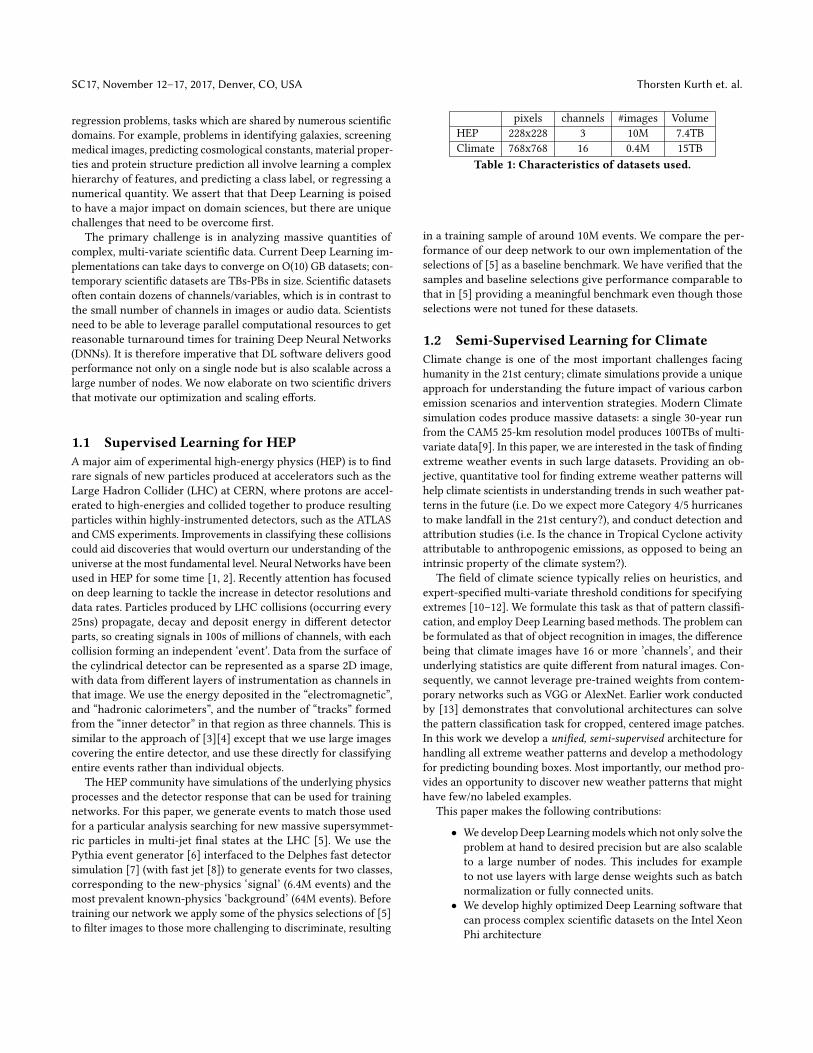
6 PERFORMANCE RESULTS6.1 Single node performanceFigures 5a and 5b show the �op rates and time spent in variouslayers for HEP and Climate networks. For a batch size of 8 images,the overall �op rate of the HEP network stands at 1.90 TFLOP/s,while that of the Climate network stands at 2.09 TFLOP/s. For bothnetworks, most of the runtime is spent in convolutional layers,which can obtain between 3.5 TFLOP/s for layers with many chan-nels, and around 1.25 TFLOP/s on the initial layers with very fewchannels. As mentioned previously in DeepBench [17], the shapesof the parameters and inputs to a layer can a�ect performancesigni�cantly; we observe that in our experiments.

3This includes the subsets F, CD, ER, PF but not VL, BW, DQ, IFMA, VBMI.

For the HEP network, about 12.5% of the runtime is spent in thesolver update routine which applies the update to the weights andadjusts hyper-parameters for the next iteration. This step spendstime in operations like copying models to keep history that do notcontribute to �ops. The overhead of this step is insigni�cant (< 2%)in the climate network. For the climate network, time spent in I/O(13%) for loading the data is signi�cant; recall that climate problemconsists of high resolution, 16-channel data. In comparison, theI/O time is much lower ( 2 %) for the HEP network, which has lowresolution, 3-channel data. We have identi�ed two bottlenecks inour current I/O con�guration: �rst, I/O throughput from a singleXeon Phi core is relatively slow, second, the current HDF5 libraryis not multi-threaded. We will address these limitations in futurework.

6.2 Multi-node scalingWe now report on scaling experiments conducts on Cori Phase II.

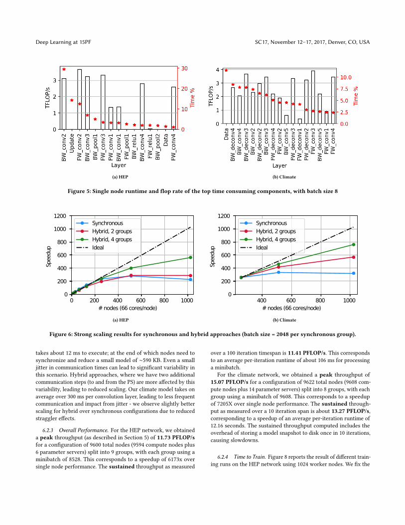
6.2.1 Strong Scaling. The strong scaling con�guration (involv-ing keeping the overall batch size per update step �xed while vary-ing the number of nodes) is a natural use-case for deep learning.Figure 6 shows the strong scaling results for HEP and climate net-works. We show 3 con�gurations: 1 synchronous group, 2 and 4hybrid groups; and show scalability from 1 to 1024 nodes. We use abatch size of 2048 per update. For the synchronous con�guration,all nodes split the batch of 2048 images; for hybrid con�gurations,each compute group independently updates the model and is as-signed a complete batch. Figure 6a shows that the synchronousalgorithm does not scale past 256 nodes – 1024 node performance issomewhat worse than for 256. The scalability improves moderatelyfor 2 hybrid groups, which saturates at 280x beyond 512 nodes, andmore signi�cantly with 4 hybrid groups, with about 580x scaling at1024 nodes. We observe similar trends for the climate network inFigure 6b - the synchronous algorithm scales only to a maximumof 320x at 512 nodes and stops scaling beyond that point. The 2 and4 group hybrid groups continue scaling to 1024 nodes; with scala-bility improving from 580x (on 1024 nodes) for 2 hybrid groups to780x for 4 hybrid groups. There are two main reasons for this: one,in hybrid algorithms, only a subset of nodes need to synchronizeat each time step; this reduces communication costs and stragglere�ects. Second, the minibatch size per node is higher for the hybridapproaches resulting in better single node performance. Scalingfor our hybrid approaches is still not linear due to the single nodeperformance drop from reduced minibatch sizes at scale.

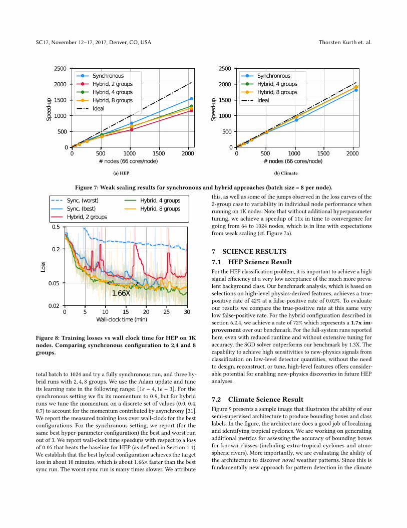
6.2.2 Weak Scaling. Figure 7a shows weak scaling for the HEPnetwork, where we keep a constant batch size (8 per node) acrossall con�gurations (synchronous and hybrid). On scaling from 1 to2048 nodes, we �nd that the performance scales sub-linearly for allcon�gurations: about 575-750x speed-up on 1024 nodes; and about1150-1250x speed-up on 2048 nodes for asynchronous con�gura-tions. We note that the synchronous speed-up on 2048 nodes standsat about 1500x. In contrast, the weak scaling results for the climatenetwork in Figure 7b are near-linear (1750x for synchronous andabout 1850x for hybrid con�gurations). Our analysis indicates sig-ni�cant variability in runtime across iterations for HEP at scale,leading to sublinear scaling. An average convolution layer in HEP


(a) HEP (b) Climate

Figure 5: Single node runtime and �op rate of the top time consuming components, with batch size 8

0 200 400 600 800 1000# nodHs (66 corHs/nodH)

0

200

400

600

800

1000

1200

6SHH

duS

6ynchronousHybrid, 2 grouSsHybrid, 4 grouSs,dHal

(a) HEP

400 600 800 1000# nodHs (66 corHs/nodH)

0

200

400

600

800

1000

12006S

HHdu

S

6ynchronousHybrid, 2 grouSsHybrid, 4 grouSs,dHal

(b) Climate

Figure 6: Strong scaling results for synchronous and hybrid approaches (batch size = 2048 per synchronous group).

takes about 12 ms to execute; at the end of which nodes need tosynchronize and reduce a small model of ⇠590 KB. Even a smalljitter in communication times can lead to signi�cant variability inthis scenario. Hybrid approaches, where we have two additionalcommunication steps (to and from the PS) are more a�ected by thisvariability, leading to reduced scaling. Our climate model takes onaverage over 300 ms per convolution layer, leading to less frequentcommunication and impact from jitter - we observe slightly betterscaling for hybrid over synchronous con�gurations due to reducedstraggler e�ects.

6.2.3 Overall Performance. For the HEP network, we obtaineda peak throughput (as described in Section 5) of 11.73 PFLOP/sfor a con�guration of 9600 total nodes (9594 compute nodes plus6 parameter servers) split into 9 groups, with each group using aminibatch of 8528. This corresponds to a speedup of 6173x oversingle node performance. The sustained throughput as measured

over a 100 iteration timespan is 11.41 PFLOP/s. This correspondsto an average per-iteration runtime of about 106 ms for processinga minibatch.

For the climate network, we obtained a peak throughput of15.07 PFLOP/s for a con�guration of 9622 total nodes (9608 com-pute nodes plus 14 parameter servers) split into 8 groups, with eachgroup using a minibatch of 9608. This corresponds to a speedupof 7205X over single node performance. The sustained through-put as measured over a 10 iteration span is about 13.27 PFLOP/s,corresponding to a speedup of an average per-iteration runtime of12.16 seconds. The sustained throughput computed includes theoverhead of storing a model snapshot to disk once in 10 iterations,causing slowdowns.

6.2.4 Time to Train. Figure 8 reports the result of di�erent train-ing runs on the HEP network using 1024 worker nodes. We �x the


0 500 1000 1500 2000# nodHs (66 corHs/nodH)

0

500

1000

1500

2000

2500

6SHH

d-uS

6ynchronousHybrid, 2 grouSsHybrid, 4 grouSsHybrid, 8 grouSs,dHal

(a) HEP

0 500 1000 1500 2000# nodHs (66 corHs/nodH)

0

500

1000

1500

2000

2500

6SHH

d-uS

6ynchronrousHybrid, 4 grouSsHybrid, 8 grouSs,dHal

(b) Climate

Figure 7: Weak scaling results for synchronous and hybrid approaches (batch size = 8 per node).

0 5 10 15 20 25 30Wall-clock WLmH (mLn)

0.02

0.05

0.2

0.5

Loss

1.66X

6ync. (worsW)6ync. (bHsW)HybrLd, 2 groXSs

HybrLd, 4 groXSsHybrLd, 8 groXSs

Figure 8: Training losses vs wall clock time for HEP on 1Knodes. Comparing synchronous con�guration to 2,4 and 8groups.

total batch to 1024 and try a fully synchronous run, and three hy-brid runs with 2, 4, 8 groups. We use the Adam update and tuneits learning rate in the following range: [1e � 4, 1e � 3]. For thesynchronous setting we �x its momentum to 0.9, but for hybridruns we tune the momentum on a discrete set of values (0.0, 0.4,0.7) to account for the momentum contributed by asynchrony [31].We report the measured training loss over wall-clock for the bestcon�gurations. For the synchronous setting, we report (for thesame best hyper-parameter con�guration) the best and worst runout of 3. We report wall-clock time speedups with respect to a lossof 0.05 that beats the baseline for HEP (as de�ned in Section 1.1).We establish that the best hybrid con�guration achieves the targetloss in about 10 minutes, which is about 1.66⇥ faster than the bestsync run. The worst sync run is many times slower. We attribute

this, as well as some of the jumps observed in the loss curves of the2-group case to variability in individual node performance whenrunning on 1K nodes. Note that without additional hyperparametertuning, we achieve a speedup of 11x in time to convergence forgoing from 64 to 1024 nodes, which is in line with expectationsfrom weak scaling (cf. Figure 7a).

7 SCIENCE RESULTS7.1 HEP Science ResultFor the HEP classi�cation problem, it is important to achieve a highsignal e�ciency at a very low acceptance of the much more preva-lent background class. Our benchmark analysis, which is based onselections on high-level physics-derived features, achieves a true-positive rate of 42% at a false-positive rate of 0.02%. To evaluateour results we compare the true-positive rate at this same verylow false-positive rate. For the hybrid con�guration described insection 6.2.4, we achieve a rate of 72% which represents a 1.7x im-provement over our benchmark. For the full-system runs reportedhere, even with reduced runtime and without extensive tuning foraccuracy, the SGD solver outperforms our benchmark by 1.3X. Thecapability to achieve high sensitivities to new-physics signals fromclassi�cation on low-level detector quantities, without the needto design, reconstruct, or tune, high-level features o�ers consider-able potential for enabling new-physics discoveries in future HEPanalyses.

7.2 Climate Science ResultFigure 9 presents a sample image that illustrates the ability of oursemi-supervised architecture to produce bounding boxes and classlabels. In the �gure, the architecture does a good job of localizingand identifying tropical cyclones. We are working on generatingadditional metrics for assessing the accuracy of bounding boxesfor known classes (including extra-tropical cyclones and atmo-spheric rivers). More importantly, we are evaluating the ability ofthe architecture to discover novel weather patterns. Since this isfundamentally new approach for pattern detection in the climate


Figure 9: Results fromplotting the network’smost con�dent(>95%) box predictions on an image for integrated water va-por (TMQ) from the test set for the climate problem. Blackbounding boxes show ground truth; Red boxes are predic-tions by the network.

science community, we do not have a well-established benchmarkto compare our results to.

8 IMPLICATIONS8.1 Deep Learning on HPCTo the best of our knowledge, ourwork is the �rst successful attemptat scaling Deep Learning on large, many-core HPC systems. Weshare a number of insights from this unique exercise.

First, at a scale of thousands of nodes, we found signi�cantvariability in runtimes across runs, which could be as high as 30%.The probability of one of the thousands of nodes failing or degradingduring the run is non-zero. In this work, we report runs where wedid not encounter complete node failures.We note that even a singlenode failure can cause complete failure of synchronous runs; hybridruns are much more resilient since only one of the compute groupsgets a�ected. However, even in hybrid runs, if model updates fromone of the compute groups lags signi�cantly behind others, it canresult in "jumps" in the overall loss and accuracy that we havehighlighted in Figure 8.

Second, current architectures and software stacks for deep learn-ing are still not as mature as the traditional HPC application stack.Speci�cally, performance on small batch sizes (essential for scaleout) has not been completely optimized in many frameworks. Fur-ther, the state of the art in deep learning kernel implementations israpidly evolving with new algorithms like Winograd [43] and FFTbased algorithms. We did not experiment with such algorithms in

this work; studying the impact on per-node performance and scaleout behaviour of these algorithms is a direction for future research.

There has been a lot of discussion surrounding training withquantized weights and activations [44, 45]. The statistical implica-tions of low precision training are still being explored [46, 47], withvarious forms of stochastic rounding being of critical importance inconvergence. While supercomputers with architectures supportinglow precision computations in hardware are not yet present, webelieve that such systems have the potential to further acceleratetraining time for our applications.

8.2 Deep Learning for ScienceWe believe that science domains that can readily generate vastamounts of representative training data (via simulators) stand tobene�t immediately from progress in DL methods. In other scien-ti�c domains, unsupervised, and semi-supervised learning are keychallenges for the future. In both cases, it is unreasonable to expectscientists to be conversant in the art of hyper-parameter tuning.Hybrid schemes, like the one presented in this paper, add an extraparameter to be tuned, which stresses the need for principled mo-mentum tuning approaches, an active area of research (eg.[25] andrecently [48]). With hyper-parameter tuning taken care of, higher-level libraries such as Spearmint [49] can be used for automatingthe search for network architectures.We also note that more aggressive optimizations involving com-puting in low-precision and communicating high-order bits ofweight updates are poorly understood with regards to their im-plications for classi�cation and regression accuracy for scienti�cdatasets. A similar story holds with regards to deployment of DLmodels. Unlike commercial applications where a sparse/compactrepresentation of the model needs to be deployed in-situ, scienti�capplications will typically utilize DL models within the context ofthe HPC/Datacenter environment. Nevertheless, the �eld of DeepLearning is evolving rapidly, and we look forward to adoptingadvances in the near future.

9 CONCLUSIONSThis paper has presented the �rst 15-PetaFLOP Deep Learning soft-ware running on HPC platforms. We have utilized IntelCa�e toobtain ⇠2 TF on single Xeon Phi nodes. We utilize a hybrid strategyemploying synchronous groups, and asynchronous communicationamong them to scale the training of a single model to ⇠9600 CoriPhase II nodes. We apply this framework to solve real-world super-vised and semi-supervised patterns classi�cation problems in HEPand Climate Science. Our work demonstrates that manycore HPCplatforms can be successfully used to accelerate Deep Learning,opening the gateway for broader adoption by the domain sciencecommunity. Our results are not limited to the speci�c applicationsmentioned in this paper, but they extend to other kinds of modelssuch as ResNets [50] and LSTM [51, 52], although the optimal con-�guration between synchronous and asynchronous is expected tobe model dependent. This highlights the importance of a �exible,hybrid architecture in achieving the best performance for a diverseset of problems.


ACKNOWLEDGMENTSThis research used resources of the National Energy Research Sci-enti�c Computing Center (NERSC). This manuscript has been au-thored by an author at Lawrence Berkeley National Laboratoryunder Contract No. DE-AC02-05CH11231 with the U.S. Depart-ment of Energy. The U.S. Government retains, and the publisher,by accepting the article for publication, acknowledges, that the U.S.Government retains a non-exclusive, paid-up, irrevocable, world-wide license to publish or reproduce the published form of thismanuscript, or allow others to do so, for U.S. Government purposes.We would like to thank Doug Jacobsen, Brandon Cook, Tina De-clerck, David Paul and Rebecca Hartman-Baker for assisting withand troubleshooting Cori reservations. We would like to acknowl-edge Christopher Beckham, Tegan Maharaj and Christopher Pal,Yunjie Liu and Michael Wehner for help with preparing the climatearchitecture and dataset. We would like to acknowledge Steve Far-rell for assistance with preparing HEP datasets and Ben Nachmanand Brian Amadio for physics input on those datasets. Christo-pher Ré’s group at Stanford was the source of valuable advice onasynchrony. We would like to thank Srinivas Sridharan, MikhailSmorkalov, Mikhail Shiryaev and Dipankar Das for their help inintegrating and modifying Intel MLSL.

REFERENCES[1] C. Peterson, “Track �nding with neural networks,” Nuclear Instruments and

Methods in Physics Research Section A: Accelerators, Spectrometers, Detectors andAssociated Equipment, vol. 279, no. 3, pp. 537 – 545, 1989.

[2] B. Denby, “Neural networks and cellular automata in experimental high energyphysics,” Computer Physics Communications, vol. 49, no. 3, pp. 429 – 448, 1988.

[3] L. de Oliveira, M. Kagan, L. Mackey, B. Nachman, and A. Schwartzman, “Jet-images – deep learning edition,” JHEP, vol. 07, p. 069, 2016.

[4] P. T. Komiske, E. M. Metodiev, and M. D. Schwartz, “Deep learning in color:towards automated quark/gluon jet discrimination,” JHEP, vol. 01, p. 110, 2017.

[5] The ATLAS collaboration, “Search for massive supersymmetric particles in multi-jet �nal states produced in pp collisions at

ps = 13 TeV using the ATLAS detector

at the LHC,” ATLAS-CONF-2016-057, 2016.[6] T. Sjöstrand, S. Mrenna, and P. Skands, “A brief introduction to PYTHIA 8.1,”

Computer Physics Communications, vol. 178, no. 11, pp. 852 – 867, 2008.[7] J. de Favereau, C. Delaere, P. Demin, A. Giammanco, V. LemaÃőtre, A. Mertens,

and M. Selvaggi, “DELPHES 3, A modular framework for fast simulation of ageneric collider experiment,” JHEP, vol. 02, p. 057, 2014.

[8] M. Cacciari, G. P. Salam, and G. Soyez, “Fastjet user manual,” The EuropeanPhysical Journal C, vol. 72, no. 3, p. 1896, 2012.

[9] M. Wehner, Prabhat, K. A. Reed, D. Stone, W. D. Collins, and J. Bacmeister,“Resolution dependence of future tropical cyclone projections of cam5.1 in theu.s. clivar hurricane working group idealized con�gurations,” Journal of Climate,vol. 28, no. 10, pp. 3905–3925, 2015.

[10] T. R. Knutson, J. L. McBride, J. Chan, K. Emanuel, G. Holland, C. Landsea, I. Held,J. P. Kossin, A. Srivastava, and M. Sugi, “Tropical cyclones and climate change,”Nature Geoscience, vol. 3, no. 3, pp. 157–163, 2010.

[11] D. A. Lavers, G. Villarini, R. P. Allan, E. F. Wood, and A. J. Wade, “The detectionof atmospheric rivers in atmospheric reanalyses and their links to british winter�oods and the large-scale climatic circulation,” Journal of Geophysical Research:Atmospheres, vol. 117, no. D20, 2012.

[12] U. Neu and et al., “Imilast: A community e�ort to intercompare extratropical cy-clone detection and tracking algorithms,” Bulletin of the American MeteorologicalSociety, vol. 94, no. 4, pp. 529–547, 2013.

[13] Y. Liu, E. Racah, Prabhat, J. Correa, A. Khosrowshahi, D. Lavers, K. Kunkel,M. Wehner, and W. D. Collins, “Application of deep convolutional neu-ral networks for detecting extreme weather in climate datasets,” CoRR, vol.abs/1605.01156, 2016.

[14] S. Chetlur, C. Woolley, P. Vandermersch, J. Cohen, J. Tran, B. Catanzaro,and E. Shelhamer, “cuDNN: E�cient primitives for deep learning,” CoRR, vol.abs/1410.0759, 2014.

[15] “Introducing DNN primitives in Intel® Math Kernel Library,” https://software.intel.com/en-us/articles/introducing-dnn-primitives-in-intelr-mkl, 2017.

[16] A. Heinecke, G. Henry, M. Hutchinson, and H. Pabst, “Libxsmm: Acceleratingsmall matrix multiplications by runtime code generation,” in Proceedings of SC16.

IEEE Press, 2016, pp. 84:1–84:11.[17] “Deepbench,” github.com/baidu-research/DeepBench, 2017.[18] D. Amodei, R. Anubhai, E. Battenberg, C. Case, J. Casper, B. Catanzaro, J. Chen,

M. Chrzanowski, A. Coates, G. Diamos et al., “Deep speech 2 : End-to-end speechrecognition in english and mandarin,” in Proceedings of ICML), 2016, pp. 173–182.

[19] J. Dean, G. Corrado, R. Monga, K. Chen, M. Devin, M. Mao, A. Senior, P. Tucker,K. Yang, Q. V. Le et al., “Large scale distributed deep networks,” in NIPS, 2012, pp.1223–1231.

[20] F. N. Iandola, K. Ashraf, M. W. Moskewicz, and K. Keutzer, “Fireca�e: near-linearacceleration of deep neural network training on compute clusters,” CoRR, vol.abs/1511.00175, 2015.

[21] D. Das, S. Avancha, D. Mudigere, K. Vaidyanathan, S. Sridharan, D. D. Kalamkar,B. Kaul, and P. Dubey, “Distributed deep learning using synchronous stochasticgradient descent,” CoRR, vol. abs/1602.06709, 2016.

[22] S. Pathak, P. He, and W. Darling, “Scalable deep document / sequencereasoning with cognitive toolkit,” in Proceedings of the 26th InternationalConference on World Wide Web Companion, ser. WWW ’17 Companion.Republic and Canton of Geneva, Switzerland: International World WideWeb Conferences Steering Committee, 2017, pp. 931–934. [Online]. Available:https://doi.org/10.1145/3041021.3051103

[23] “Scaling Deep Learning on 18,000 GPUs,” https://www.nextplatform.com/2017/03/28/scaling-deep-learning-beyond-18000-gpus/, 2017.

[24] A. Anandkumar. Deep Learning at Scale on AWS. [Online]. Available: https://ml-days-prd.s3.amazonaws.com/slides/speakers/slides/3/Anima-EPFL2017.pdf

[25] S. Hadjis, C. Zhang, I. Mitliagkas, D. Iter, and C. Ré, “Omnivore: An optimizerfor multi-device deep learning on cpus and gpus,” arXiv:1606.04487, 2016.

[26] N. S. Keskar, D. Mudigere, J. Nocedal, M. Smelyanskiy, and P. T. P. Tang, “Onlarge-batch training for deep learning: Generalization gap and sharp minima,”arXiv:1609.04836, 2016.

[27] J. Tsitsiklis, D. Bertsekas, andM. Athans, “Distributed asynchronous deterministicand stochastic gradient optimization algorithms,” IEEE transactions on automaticcontrol, vol. 31, no. 9, pp. 803–812, 1986.

[28] F. Niu, B. Recht, C. Re, and S. Wright, “Hogwild: A lock-free approach to paral-lelizing stochastic gradient descent,” in NIPS, 2011, pp. 693–701.

[29] J. Dean, G. Corrado, R. Monga, K. Chen, M. Devin, M. Mao, A. Senior, P. Tucker,K. Yang, Q. V. Le et al., “Large scale distributed deep networks,” in NIPS, 2012, pp.1223–1231.

[30] T. Chilimbi, Y. Suzue, J. Apacible, and K. Kalyanaraman, “Project adam: Buildingan e�cient and scalable deep learning training system,” in 11th USENIX Sym-posium on Operating Systems Design and Implementation (OSDI 14), 2014, pp.571–582.

[31] I. Mitliagkas, C. Zhang, S. Hadjis, and C. Ré, “Asynchrony begets momentum,with an application to deep learning,” arXiv:1605.09774, 2016.

[32] C. Zhang and C. Re, “Dimmwitted: A study of main-memory statistical analytics,”PVLDB, vol. 7, no. 12, pp. 1283–1294, 2014.

[33] R. H. Hahnloser, R. Sarpeshkar, M. A. Mahowald, R. J. Douglas, and H. S. Seung,“Digital selection and analogue ampli�cation coexist in a cortex-inspired siliconcircuit,” Nature, vol. 405, no. 6789, pp. 947–951, 2000.

[34] K. He, X. Zhang, S. Ren, and J. Sun, “Delving deep into recti�ers: Surpassinghuman-level performance on imagenet classi�cation,” in Proceedings of ICCV,2015, pp. 1026–1034.

[35] D. Kingma and J. Ba, “Adam: A method for stochastic optimization,”arXiv:1412.6980, 2014.

[36] E. Racah, C. Beckham, T. Maharaj, C. Pal et al., “Semi-supervised detection ofextreme weather events in large climate datasets,” arXiv:1612.02095, 2016.

[37] J. Redmon, S. Divvala, R. Girshick, and A. Farhadi, “You only look once: Uni�ed,real-time object detection,” in CVPR, 2016, pp. 779–788.

[38] W. Liu, D. Anguelov, D. Erhan, C. Szegedy, S. Reed, C.-Y. Fu, and A. C. Berg,“Ssd: Single shot multibox detector,” in European Conference on Computer Vision.Springer, 2016, pp. 21–37.

[39] S. Ren, K. He, R. Girshick, and J. Sun, “Faster r-cnn: Towards real-time objectdetection with region proposal networks,” in NIPS, 2015, pp. 91–99.

[40] “Intel® distribution of Ca�e*,” https://github.com/intel/ca�e, 2017.[41] “Intel® Machine Learning Scaling Library for Linux* OS,” https://github.com/

01org/MLSL, 2017.[42] “Intel® Software Development Emulator,” https://software.intel.com/en-us/

articles/intel-software-development-emulator, 2017.[43] A. Lavin and S. Gray, “Fast algorithms for convolutional neural networks,” CoRR,

vol. abs/1509.09308, 2015.[44] I. Hubara, M. Courbariaux, D. Soudry, R. El-Yaniv, and Y. Bengio, “Quantized

neural networks: Training neural networks with low precision weights andactivations,” CoRR, vol. abs/1609.07061, 2016.

[45] M. Courbariaux, Y. Bengio, and J. David, “Training deep neural networks withlow precision multiplications,” CoRR, vol. abs/1412.7024, 2014.

[46] S. Gupta, A. Agrawal, K. Gopalakrishnan, and P. Narayanan, “Deep learningwith limited numerical precision,” CoRR, vol. abs/1502.02551, 2015.


[47] P. Gysel, M. Motamedi, and S. Ghiasi, “Hardware-oriented approximation ofconvolutional neural networks,” CoRR, vol. abs/1604.03168, 2016.

[48] J. Zhang, I. Mitliagkas, and C. Ré, “Yellow�n and the art of momentum tuning,”arXiv preprint arXiv:1706.03471, 2017.

[49] J. Snoek, H. Larochelle, and R. P. Adams, “Practical bayesian optimization ofmachine learning algorithms,” in NIPS, 2012, pp. 2951–2959.

[50] K. He, X. Zhang, S. Ren, and J. Sun, “Deep residual learning for image recognition,”in Proceedings of the IEEE conference on computer vision and pattern recognition,2016, pp. 770–778.

[51] S. Hochreiter and J. Schmidhuber, “Long short-term memory,” NeuralComputation, vol. 9, no. 8, pp. 1735–1780, 1997. [Online]. Available:http://dx.doi.org/10.1162/neco.1997.9.8.1735

[52] F. A. Gers, J. Schmidhuber, and F. Cummins, “Learning to forget: Continualprediction with lstm,” Neural Computation, vol. 12, no. 10, pp. 2451–2471, 2000.[Online]. Available: http://dx.doi.org/10.1162/089976600300015015

Deep Learning at 15PF - University of Southern...

Documents

Transcript of Deep Learning at 15PF - University of Southern...